The risk prediction of Alzheimer’s disease based on the deep learning model of brain 18F-FDG positron emission tomography

Abstract

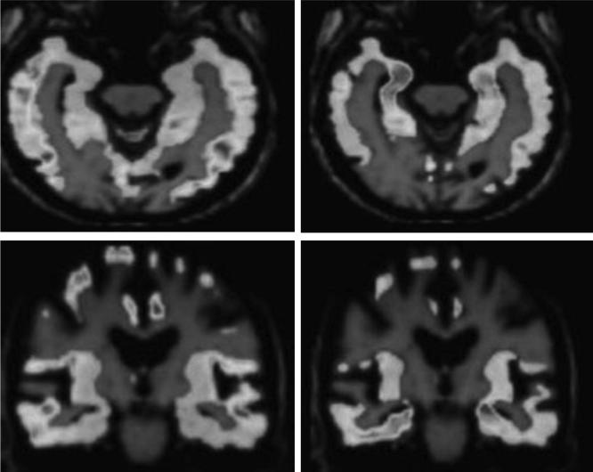
In order to predict the risks of Alzheimer’s Disease (AD) based on the deep learning model of brain 18F-FDG positron emission tomography (PET), a total of 350 mild cognitive impairment (MCI) participants from the Alzheimer’s Disease Neuroimaging Initiative (ADNI) database were selected as the research objects; in addition, the Convolutional Architecture for Fast Feature Embedding (CAFFE) was selected as the framework of the deep learning platform; the FDG PET image features of each participant were extracted by a deep convolution network model to construct the prediction and classification models; therefore, the MCI stage features were classified and the transformation was predicted. The results showed that in terms of the MCI transformation prediction, the sensitivity and specificity of conv3 classification were respectively 91.02% and 77.63%; in terms of the Late Mild Cognitive Impairment (LMCI) and Early Mild Cognitive Impairment (EMCI) classification, the accuracy of conv5 classification was 72.19%, and the sensitivity and specificity of conv5 were all 73% approximately. Thus, it was seen that the model constructed in the research could be used to solve the problems of MCI transformation prediction, which also had certain effects on the classifications of EMCI and LMCI. The risk prediction of AD based on the deep learning model of brain 18F-FDG PET discussed in the research matched the expected results. It provided a relatively accurate reference model for the prediction of AD. Despite the deficiencies of the research process, the research results have provided certain references and guidance for the future exploration of accurate AD prediction model; therefore, the research is of great significance.

1. Introduction

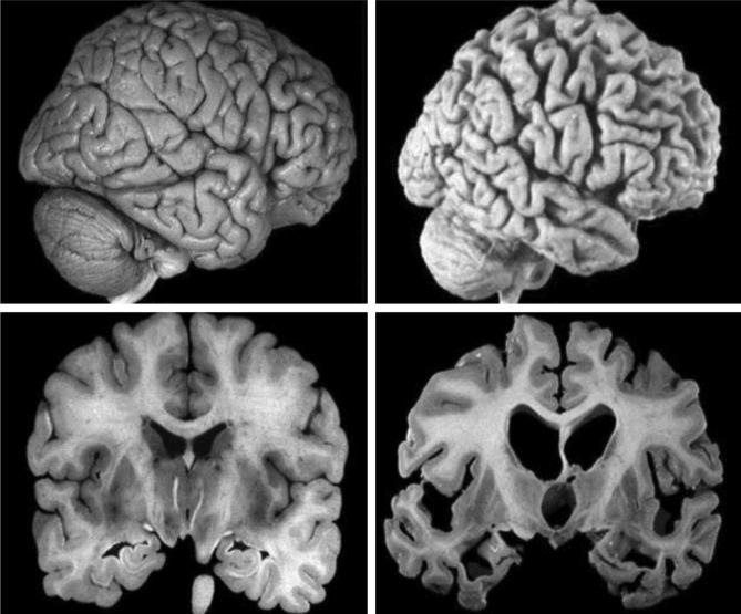
Alzheimer’s Disease (AD) is a chronic neurodegenerative disease whose clinical manifestations are mainly memory degradation and cognitive function impairment, which seriously threatens the quality and safety of life of the seniors (Coleman et al., 2017). Fig. 1 shows the brains of AD patients presented by tomography. Research has suggested that the incidence rate of dementia among seniors over 65 years old in European and American countries is about 4–8%, while the incidence rate of dementia in China is 7.8%, in which the incidence rate of AD is 4.8% (Smailagic et al., 2018). As the country with the largest population in the world, China is about to face the increasingly serious problem of population aging, and AD would bring enormous economic and living burdens to patients, families, and the society (Oliveira et al., 2018).

Fig. 1.

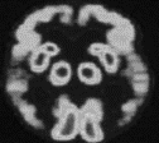
Brains of AD patients presented by tomography.

Based on the malignant degradation of cognitive and physical functions of patients, clinically, AD is divided into 3 stages, i.e. the pre-clinical stage, the mild cognitive function impairment stage, and the dementia stage (Jiang et al., 2018). In the pre-clinical stage, the early pathological onset of the disease begins in the cerebral cortex, cerebrospinal fluid (CSF), and blood circulation of the patient; however, no significant clinical manifestations are observed, as shown in Fig. 2. Mild cognitive impairment (MCI) is a transitional stage between normal aging and the progression to AD. The thinking ability and memory of MCI patients are degraded mildly, which would affect the daily communication of MCI patients (Ma et al., 2018). A survey has suggested that about 10–15% MCI patients are progressed to AD annually, while the transformation rate of AD among normal seniors is only 1–2%; in addition, the transformation rate of MCI in 4–6 years is about 40–60.92% (Malpetti et al., 2017). Thus, it is seen that MCI is more likely to be further developed into AD, which can be used as a key breakthrough in the early diagnosis of AD.

Fig. 2.

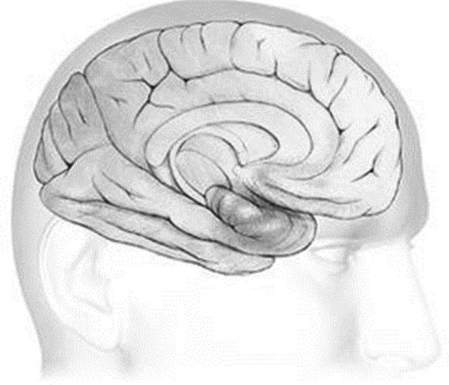
The schematic diagram of the brain at the initial stage of AD.

At present, the clinical examination methods of AD mainly include cerebrospinal fluid examination, electroencephalogram examination, neuropsychological examination, neuroimaging examination, and the latest genetic detection and molecular probe detection. Neuroimaging is widely used in the field of assisted diagnosis for the cerebral disease. It can provide rich information about brain structure or brain functions and help researchers analyze the conditions of patients from various angles, making the early diagnosis of cerebral disease possible (Ferreira et al., 2017). Therefore, MCI is an important point of penetration for the early diagnosis and prevention of AD. Based on the deep learning network model, a risk prediction model of AD was proposed in the research to predict the transformation of AD from MCI in advance, thereby effectively reducing the incidence rate of AD. Due to the difference in the types of data structures and the degrees of complexity, the prediction effects obtained by different prediction models applied to different fields are also different. According to the information obtained in the previous documents, the widely used prediction models in the imaging field include the support vector machine and Lasso. The texture data of medical images have strong self-characteristics, including large data dimensions, large data variables, and a certain weak correlation between variables. To improve the risk prediction rate of AD, this study will further explore the key aspects of AD risk prediction based on the theoretical basis of deep learning and the 18F-FDG PET image data of the brain.

2. Materials and methods

A total of 350 mild cognitive impairment (MCI) participants from the ADNI database were selected as the research objects; in addition, the CAFFE was selected as the framework of the deep learning platform, the FDG PET image features of each participant were extracted by a deep convolution network model; then, a risk prediction model of AD was constructed to predict the transformation of AD from MCI in the hope of reducing the incidence rate of AD.

2.1. ADNI and research objects

The Alzheimer’s Disease Neuroimaging Initiative (ADNI) is a global longitudinal multi-site observational study based on various approaches such as comprehensive neuroimaging examinations, assays of CSF and blood biomarkers, and clinical cognitive function assessments, which aims to identify AD at an earlier stage and provide evidence for early diagnosis and treatment of AD.

Research carried out in the ADNI database is divided into 3 stages, i.e. ADNI1, ADNI-GO, and ADNI2. The first stage (ADNI1) was completed in October 2010. Completion institutions included a total of 57 research centers in the United States and Canada, with a total of 819 research objects included, in which 192 cases were AD patients, 398 cases were mild cognitive impairment (MCI) patients and 229 were normal aging populations. Fig. 3 compares the brain scans between healthy people and AD patients.

Fig. 3.

Brain scans of healthy people and AD patients (the left image shows the brain of healthy people; the right image shows the brain of AD patients).

After the completion of the first stage ADNI1, a two-year study was continued, which became the second stage ADNI-GO, with new patients added. The third stage is the ADNI2 stage. The respective inclusion criteria of each group in the ADNI-GO and ADNI2 stages are as follows:

The normal control group (NC): The score of Mini-Mental State Examination (MMSE) is between 24 and 30 points, and the Clinical Dementia Rating (CDR) score is 0 points; in order to avoid the potential incidence risks of AD or MCI among the objects in the group, all the objects should be 70-year-old seniors. The tracking acquisition time is 0, 3, 6, 12, 24, and 36 months.

The EMCI group: The MMSE score (Liu et al., 2018) is between 24 and 30 points, with complaints of memory impairment; in terms of the scores obtained from the Logical Memory Assessment Scale in the Delayed Memory Scale (Rondina et al., 2018), the one whose education years exceed 16 years would get 9–11 points, the one whose education years are 8–15 years would get 5–9 points, and the one whose education years are 0–7 years would get 3–6 points, the CDR score is 0.5, the patient could take care of himself/herself in daily life, no obvious symptoms of dementia are seen. The tracking acquisition time of newly included objects in ADNI-GO is 0, 3, 6, and 12 months. The tracking acquisition time of newly included objects in ADNI2 is 0, 3, 6, 12, 24, and 36 months.

The LMCI group: The difference from EMCI is that it compares the degree of education with the loss of objective memory; the one whose education years exceed 16 years would get a maximum of 8 points, the one whose education years are 8–15 years would get 5–9 points, and the one whose education years are 0–7 years would get 3–6 points, and the other assessment criteria are the same as that of the EMCI group.

In the research, a total of 350 MCI participants from the ADNI database were selected as the research objects to analyze their FDG positron emission tomography (PET) images. Based on the research needs and the follow-up records of the ADNI, all the 350 MCI participants were divided into MCIc and MCInc; information of the participant is summarized in Table 1.

Table 1.

Information on research objects.

	MCIc	MCInc
Total number	70	280
Gender (male/female)	32/38	143/137
Age (yr)	71.7 ± 5.8	72.0 ± 5.9
Educational level	16.0 ± 2.4	16.3 ± 2.6
MMSE	27.1 ± 1.7	27.8 ± 1.5

2.2. Deep learning framework

Based on actual needs, the CAFFE was selected as the framework of the deep learning platform. CAFFE was implemented in C++ language and had Python and Matlab interfaces; it could quickly realize the convolution neural network (CNN) on GPU and conveniently convert between GPU and CPU. CAFFE had visual interfaces in the Linux operating environment, which provided a relatively sophisticated tool for the visualization of the deep network.

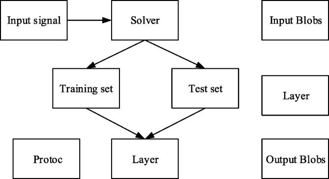
The 3 basic results of the CAFFE framework were Blobs, Layers, and Nets. The function of Blobs was to store and distribute various data; common Blobs were 4D vectors, including the “Number” that represented the number of images and the “Channel” that represented the color channels of images, where the channel of the grayscale image was 1 and the channel of the 3-channel RGB was 3; in addition, “Height” and “Width” were used to indicate the heights and widths of images respectively (Purandare et al., 2017).

In the implementation process, CAFFE generally included the network layer and the pooling layer; the “Layers” are the basis for the realization of functions of various layers, which generally included 3 steps, i.e. the construction of layers, the forward propagation, and the back-propagation (BP). “Nets” generally consisted of multiple layers, which defined the entire network results as input and output, etc.; it was the integration of multiple “Layer” layers to form a complete network result. The operating principles of the CAFFE framework are illustrated in Fig. 4.

Fig. 4.

Operating principles of CAFFE framework.

2.3. Deep convolution network model and AlexNet

In the research, the CNN network structure was trained by the combination of neural cognitive machine and BP algorithm; the LeNet-5 model was used as the deep convolution network model; the network structure was illustrated in Fig. 5.

Fig. 5.

Convolution process of LeNet-5.

The general network structure of a convolution neural network (CNN) consists of an input layer, a convolution layer, a pooling layer, a full connected layer, and an output layer (Inui et al., 2017).

Usually, each convolution layer was composed of several feature surfaces, and each feature surface had plenty neurons, which were locally connected to the input to extract the local features; meanwhile, each feature surface was interconnected and affected the relations with other feature spaces, and multiple feature maps would form new feature surfaces.

In the process of convolution calculation, the convolution kernel was connected to a local region of the feature map, which was called the local receptive field. The weight of the convolution kernel shared by the entire feature map was called weight sharing. The convolution-calculated feature maps could be expressed through Eq. (1):

$$X_j^{\text{l}}=f\left(\sum _{\text{i}\in M^j}{X}_i^{l-1}\times k_{\mathit{ij}}^l+b_j^i\right)$$ (1)

The output of the convolution layer was permitted by locally weighting and transferring to a nonlinear activation function (such as Sigmoid). Currently, the activation functions could be roughly divided into Sigmoid functions and non-Sigmoid functions, the LeNet-5 used Sigmoid functions, which was expressed as Eq. (2)

$$f\left(x\right)=\frac{1}{1+e^x}$$ (2)

Generally, the convolution layer was closely followed by the pooling layer, which was also composed of several feature surfaces, and each feature surface shared a unique correspondence relationship with the feature surface of the convolution layer; in addition, the pooling layer also had the features of weight sharing and local connection, and the main function was to reduce the dimensionality of images while preserving the original feature information of images, thereby the number of parameters during network training was reduced. The network after dimensionality reduction not only reduced the computational complexity and the complexity of the hidden layer but also made it easier to classify. The general form of pooling was expressed by Eq. (3);

$$X_j^{\text{l}}=f\left(w_j^{l}down(X_j^{(l-1)})+b_j^i\right)$$ (3)

The pooling methods adopted in the research were max pooling and average pooling. The pooling process was similar to the convolution process, which moved in the order of from the top to the bottom and from the left to the right. Max Pooling found the maximum value of the covered window as an element of the output feature map; Average Pooling found the average value of the covered window as an element of the output feature map. Pooling was important for processing images with different sizes in actual problems; since the classification layer must be uniformly fixed, the image size could be unified by adjusting the paranoid size of the pooling layer.

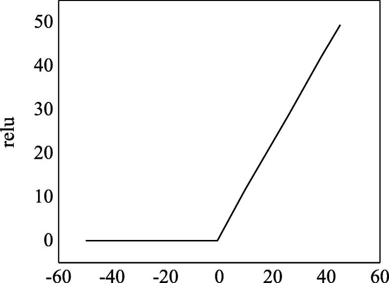
The network structure of AlexNet included 8 layers of neural networks, 5 convolution layers, and 3 full connected layers. Given the enormous data and network scale, it was necessary to put forward higher requirements for GPU video memory; therefore, the AlexNet selected 2 GTX580 GPUs in parallel, and the video memory of each GPU was 3 GB. The activation function of AlexNet was Rectified Linear Unit (ReLU), which was expressed through Eq. (4):

$$f\left(x\right)=max\left(0,x\right)$$ (4)

Compared with the saturated nonlinear activation functions such as Sigmoid and tanh, ReLU not only solved the problems of gradient explosion and disappearance but also greatly improved the convergence speed. The image of ReLU function was illustrated in Fig. 6. In the dataset of Cifar-10, once the error rate of the convolution of the 4th layer in AlexNet reduced to 25%, the convergence speed of ReLU was nearly 6 times faster than the convergence speed of $f\left(x\right)=\left|tanh\left(x\right)\right|$, which showed that ReLU greatly improved the learning efficiency.

Fig. 6.

The schematic diagram of ReLU function.

2.4. Image data processing based on CAFFE and AlexNet

The obtained image data were preprocessed; the detailed processing steps were as follows:

The PET images in the ADNI database were collected by using the PET scanners manufactured by General Electric (GE), Siemens, and Philips. Before the image collection, researchers should confirm that all participants had none of the following contraindications: (1) unable to complete the experiment (claustrophobia, etc.); (2) unable to lie on the scanning bed for 45 min (non-quantitative study) or 75 min (quantitative study); (3) unable to be injected with tracers through venous accesses. Participants who were scanned in the morning should fast until the scans were completed (with free access to water); participants who were scanned in the afternoon should fast for more than 4 h. The correct positioning of participants was a critical step to complete the PET scans; in addition, it was necessary to ensure the accuracy of the positions and the comfort of the participants. Besides, participants should leave their personal belongings out of the scan room, such as wallets, keys, glasses, necklaces, earrings, and hearing aids, etc. Additional mats were placed under the neck of the participant to provide adequate support. A laser was used to ensure no rotations in each plane. The head of the participant should be approximately parallel to the imaginary line between the outer corner of the eye and the outer ear canal. Supporting devices were provided for the back and lower limb areas. In the quantitative study, it would be better to place a small table at the edge of the scanning bed for tracer management and venous blood draw, as well as for the participant to rest. In addition, an emergency button should be provided to the participant, or a researcher was required to accompany the participant to ensure the safety of the experiment. Environmental standardization was essential within 20–30 min after the injection of 5 + 0.5 mCi (185 MBq) of the 18F-FDG tracer. During the tracer ingestion stage, participants should remain still and awake, with their eyes widely opened and looked straight ahead. The lights should be dim remained unchanged throughout the overall acquisition process. The participants were checked regularly to ensure their eyes were open and they were conscious.

The grid of voxel image re-sampled by the baseline PET image registration averaged image of each participant was oriented such that the front and rear axes of the participant were parallel to the AC-PC line. Afterward, feature extraction was performed to the preprocessed FEG-PET images. Feature extraction was an important step in the study of classification problems, which directly related to the results of classification. The feature extraction of general FDG PET images was mainly for the images themselves, including the voxel or the metabolic intensity of the brain region. In addition, the histogram and the gray level concurrence matrix (GLCM) of the gradient and direction were extracted from FDG PET images as the features in some studies. After data preprocessing, the dimension of the gray matter density map of each participant became 121 × 145 × 121, and the voxel size became a gray matter image of 1.5 × 1.5 × 1.5 mm³; however, the application of AlexNet migration learning needed to satisfy the RGB 3-channel colored images whose sides were the same as those of the input images; therefore, the pre-processed gray matter images should be converted before the features were extracted by using the migration learning method.

The image processing steps in the stage were implemented in the Windows 7 operating system by using the NifTi_2014 toolkit loaded by MRIcro software and Matlab 2015b; the first 3 steps were an interpolation, completion, and segmentation. After the 3rd step was output, the NifTi image of each participant was segmented averagely from the Z-axis into 65 images in PNG format. Finally, all the grayscale images in the PNG format were converted into pseudo-colored images in the RGB format. The parameter variations of the above-mentioned image conversion dimensions and voxels were summarized in Table 2.

Table 2.

Image-transformed parameters based on CAFFE and AlexNet.

	Original images	Step I	Step II	Step III	Step IV	Step V
Dimension changes	121 × 145 × 121	121 × 145 × 121	121 × 145 × 121	121 × 145 × 121	121 × 145 × 121	121 × 145 × 121
Voxel size (mm3)	1.5 × 1.5 × 1.5	1.5 × 1.5 × 1.5	1.5 × 1.5 × 1.5	1.5 × 1.5 × 1.5	1.5 × 1.5 × 1.5	1.5 × 1.5 × 1.5
Bytes occupied (bit)	32	32	32	32	32	32
Image format	NifTi	NifTi	NifTi	NifTi	NifTi	NifTi

After the data were prepared, all the images were transformed into Lightning Memory-Mapped Database (LMDB) format. The feature extraction process used the pre-trained CAFFE model, which required to customize the primary input parameters such as the size of the network; afterward, the different layers were selected based on to the network structure to extract features respectively; in addition, the features were extracted into LMDB format. After the features were extracted, based on the output parameters of each layer in the network model, the feature rows were visualized.

According to the principle of feature migration, each preprocessed brain image was visualized in the feature extraction of conv1, conv3, conv4, and conv5 of AlexNet, respectively. In the research, the features of conv3, conv4, and conv5 were extracted, and the features of the LMDB format were changed into feature matrices for subsequent classification and prediction. Taking conv3 as an example, according to the model parameters of AlexNet, the image of each participant became data in 65 × 64,896 dimensions, of which 64,896 was the output of conv3 13 × 13 × 384; however, in terms of the next step of classification, the image of each participant was recombined in 3D, and the dimensions reached 4,218,240, which was undoubtedly a dimensional disaster for the classifier; therefore, the features of each participant were submitted to dimension reduction by overlapping polling, in which the step was 2, the size of pooling window was 3, i.e. S = 2, Z=; then, the conv3 and conv4 feature dimensions of each participant became 1 × 898,560, and the conv5 feature dimension of each participant became 1 × 599,040.

2.5. Model construction of prediction and classification

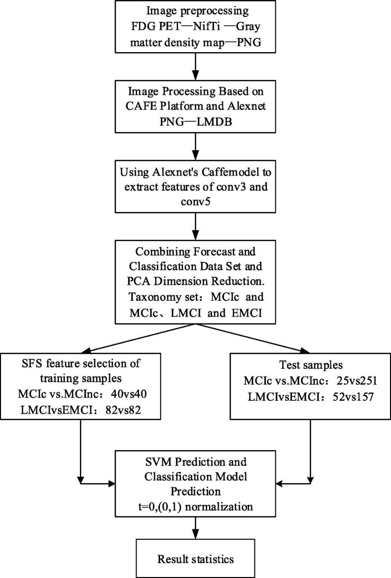
The basic construction flow of the classification and prediction model was illustrated in Fig. 7. During the image preprocessing process, the original FDG PET image was converted into NifTi format, and the gray matter was extracted to generate the gray matter density map; after the completion and segmentation, the image was converted to fit the input size of AlexNet; next, the image was converted into 2D image in PNG format, which was then converted into the LMDB format that CAFFE could recognize. During the AlexNet-based feature extraction process, features were sequentially extracted by setting input sizes and input batches that met the experimental requirements and the video memory. Afterward, the predictive model for MCIc and MCInc was constructed, and a feature classification set for the classification models of EMCI and LMCI was established. The PCA was input for dimension reduction; the training set was selected by using the SFS algorithm, and a total of 20 most representative features of the training set were selected. Since only 70 cases of MCIc were included, 40 cases were selected as the training sets in the prediction model. Finally, the selected features were input into the classifier as the test set to obtain the final classification results.

Fig. 7.

The flowchart of transformation prediction and classification methods.

3. Results and discussion

3.1. Brain PET images of MCI participants

After the tracer was ingested, the brains of the MCI participants were scanned with PET and were compared with the brain PET scans of the healthy participants. As shown in Fig. 8, compared with the healthy human brain, the brains of MCI participants began to shrink, and part of the nervous system functions would gradually degenerate.

Fig. 8.

Comparison of brain PET scans between healthy participants and MCI participants after tracer injections (The left showed the healthy human brain; the right showed the MCI brain).

3.2. Results of MCI transformation prediction model

Based on the workflow of classification and prediction models, the statistics of MCIc and MCInc classification results in each layer were summarized in Table 3.

Table 3.

Feature dimensions before and after PCA.

	Conv3		Conv5
Grouped by	Pre-PCA dimension	Post-PCA dimension	Pre-PCA dimension	Post-PCA dimension
MCIc/MCInc	351 × 898470	351 × 305	351 × 598270	351 × 201

Based on the workflow of classification and prediction models, after the SFS feature selection and SVM classifier were applied, the classification results were summarized in Table 4.

Table 4.

Classification results of MCI in each layer.

Grouped by	Layer name	TP	FP	TN	FN	Accuracy (%)	Sensitivity (%)	Specificity (%)
MCIc/MCInc	conv3	18	3	189	57	78.56	91.02	77.63
	conv5	15	6	185	62	73.91	77.54	75.11

As shown in Table 4, the classification of conv3 achieved preferable results in MCI transformation prediction, with the sensitivity and specificity being respectively 91.02% and 77.63%, which indicated that the model constructed in the research could be used to solve the MCI transformation problems.

The 3 indicators of the conv5 layer were not as preferable as those of conv3 in terms of MCI transformation prediction, which indicated that conv3 was more suitable for the construction of such transformation prediction models. The set of constructed models had a problem that the data set was very uneven; only 70 cases were included in MCIc, which may affect the accuracy of the model.

The problems of MCI transformation in the research were all based on the long-term collection of ADNI-GO and ADNI2; in addition, participants transformed from MCI to AD on a regular basis of time were unclassified; however, most previous studies would perform quantitative analysis to the MCI transformation in 3 months, 6 months, and 18 months. In addition to the time limit of the research, only 70 cases of MCIc were selected from ADNI-GO and ADNI-2; if the transformation prediction was performed, the amount of data in each group may be smaller, which would lead to more uneven data and eventually affected the classifier to a large extent.

3.3. Results of EMCI and LMCI classification models

Based on the workflow of classification and prediction models, the statistics of EMCI and LMCI classification results in each layer were summarized in Table 5.

Table 5.

Feature dimensions before and after PCA.

	Conv3		Conv5
Grouped by	Pre-PCA dimension	Post-PCA dimension	Pre-PCA dimension	Post-PCA dimension
EMCI/LMCI	351 × 898470	351 × 178	351 × 598270	351 × 201

Based on the workflow of classification and prediction models, after the SFS feature selection and SVM classifier were applied, the classification results were summarized in Table 6.

Table 6.

Classification results of MCI in each layer.

Grouped by	Layer name	TP	FP	TN	FN	Accuracy (%)	Sensitivity (%)	Specificity (%)
EMCI/LMCI	conv3	33	14	107	51	68.37	78.63	68.49
	conv5	30	15	113	46	72.19	73.82	73.05

Few binary classification problems in the LMCI and EMCI problems were discussed; currently, most of the studies were based on brain structure changes in these2 stages; the reason may be that no differences in brain structure between the 2 stages were found; therefore, no conclusions were drawn, and no strict ROI feature extraction methods could be applied to construct the classification model. In the research, the full brain gray matter features were used as the materials for feature extraction. As for the classification problems of LMCI and EMCI in the conv5 layer, the accuracy was 72.19%, and the sensitivity and specificity were all 73% approximately, indicating that the classification model was useful to the classification of EMCI and LMCI.

4. Conclusion

The positron emission tomography (PET) is an advanced nuclear medicine functional imaging technology used to observe metabolic processes in vivo to help clinicians diagnose diseases. A total of 350 mild cognitive impairment (MCI) participants from the ADNI database were selected as the research objects; in addition, the CAFFE was selected as the framework of the deep learning platform, the FDG PET image features of each participant were extracted by a deep convolution network model. Then, a prediction and classification model of AD was constructed and was applied to the MCI stage, which achieved preferable classification and transformation prediction results.

The risk prediction of AD based on the deep learning model of brain 18F-FDG PET discussed in the research matched the expected results, which achieved preferable predictive results in the problem of MCI transformation. According to the prediction results, the classification of conv3 achieved good results in MCI transformation prediction, and the sensitivity and specificity were respectively 91.02% and 77.63%, indicating that the model constructed in this study can be used in the MCI transformation. In addition, by using the whole-brain gray matter feature as the material for feature extraction, 72.19% of accuracy was obtained in the classification problem of LMCI and EMCI in the conv5 layer, and the sensitivity and specificity were also about 73%, indicating that the classification model was effective for the classification of EMCI and LMCI. It provided a relatively accurate reference model for the prediction of AD. However, certain deficiencies were found in the research process, such as the limited database data, which led to the results that the accuracy of the constructed model was not well-verified. Therefore, it is necessary to increase the data capacity to further explore the accuracy of the AD risk prediction model in subsequent research.

References

- Coleman R.A., Liang C., Patel R. Brain and brown adipose tissue metabolism in transgenic Tg2576 mice models of Alzheimer disease assessed using 18F-FDG PET imaging. Mol. Imaging. 2017;16(98):1–9. doi: 10.1177/1536012117704557. [DOI] [PMC free article] [PubMed] [Google Scholar]
- Smailagic N., Lafortune L., Kelly S. 18F-FDG PET for prediction of conversion to Alzheimer’s disease dementia in people with mild cognitive impairment: an updated systematic review of test accuracy. J. Alzheimers Dis. Jad. 2018;64(4):1175–1194. doi: 10.3233/JAD-171125. [DOI] [PMC free article] [PubMed] [Google Scholar]
- Oliveira Francisco P.M., Moreira Ana Paula, de Mendonça Alexandre. Can11C-PiB-PET relative delivery R1or11C-PiB-PET perfusion replace18F-FDG PET in the assessment of brain neurodegeneration. J. Alzheimers Dis. 2018;65(1):89–97. doi: 10.3233/JAD-180274. [DOI] [PMC free article] [PubMed] [Google Scholar]
- Jiang J., Sun Y., Zhou H. Study of the influence of age in 18F-FDG PET images using a data-driven approach and its evaluation in Alzheimer’s disease. Contrast Media Mol. Imaging. 2018;2018(2):1–16. doi: 10.1155/2018/3786083. [DOI] [PMC free article] [PubMed] [Google Scholar]
- Ma H.R., Sheng L.Q., Pan P.L. Cerebral glucose metabolic prediction from amnestic mild cognitive impairment to Alzheimer’s dementia: a meta-analysis. Transl. Neurodegen. 2018;7(1):9. doi: 10.1186/s40035-018-0114-z. [DOI] [PMC free article] [PubMed] [Google Scholar]
- Malpetti M., Ballarini T., Presotto L. Gender differences in healthy aging and Alzheimer’s dementia: a 18 F-FDG PET study of brain and cognitive reserve. Hum. Brain Mapp. 2017;38:4212–4227. doi: 10.1002/hbm.23659. [DOI] [PMC free article] [PubMed] [Google Scholar]
- Ferreira L.K., Rondina J.M., Kubo R. Support vector machine-based classification of neuroimages in Alzheimer’s disease: direct comparison of FDG PET, rCBF-SPECT and MRI data acquired from the same individuals. Revista Brasileira De Psiquiatria. 2017;40(AHEAD):181–191. doi: 10.1590/1516-4446-2016-2083. [DOI] [PMC free article] [PubMed] [Google Scholar]
- Liu M., Cheng D., Yan W. Classification of Alzheimer’s disease by combination of convolutional and recurrent neural networks using FDG PET images. Front. Neuroinf. 2018;12:35. doi: 10.3389/fninf.2018.00035. [DOI] [PMC free article] [PubMed] [Google Scholar]
- Rondina J.M., Ferreira L.K., De F.S.D. Selecting the most relevant brain regions to discriminate Alzheimer’s disease patients from healthy controls using multiple kernel learning: a comparison across functional and structural imaging modalities and atlases. Neuroimage Clin. 2018;17:628–641. doi: 10.1016/j.nicl.2017.10.026. [DOI] [PMC free article] [PubMed] [Google Scholar]
- Purandare N.C., Puranik A., Shah S. Common malignant brain tumors: can 18F-FDG PET/CT aid in differentiation. Nucl. Med. Commun. 2017;38(12):1. doi: 10.1097/MNM.0000000000000753. [DOI] [PubMed] [Google Scholar]
- Inui Y., Ito K., Kato T. Longer-term investigation of the value of 18F-FDG PET and magnetic resonance imaging for predicting the conversion of mild cognitive impairment to Alzheimer’s disease: a multicenter study. J. Alzheimers Dis. 2017;60(3):877–887. doi: 10.3233/JAD-170395. [DOI] [PMC free article] [PubMed] [Google Scholar]