BornAgain: software for simulating and fitting grazing-incidence small-angle scattering

BornAgain is a free and open-source multi-platform software framework for simulating and fitting X-ray and neutron reflectometry, off-specular scattering, and grazing-incidence small-angle scattering (GISAS). This paper concentrates on GISAS.

Abstract

BornAgain is a free and open-source multi-platform software framework for simulating and fitting X-ray and neutron reflectometry, off-specular scattering, and grazing-incidence small-angle scattering (GISAS). This paper concentrates on GISAS. Support for reflectometry and off-specular scattering has been added more recently, is still under intense development and will be described in a later publication. BornAgain supports neutron polarization and magnetic scattering. Users can define sample and instrument models through Python scripting. A large subset of the functionality is also available through a graphical user interface. This paper describes the software in terms of the realized non-functional and functional requirements. The web site https://www.bornagainproject.org/ provides further documentation.

1. Introduction  

X-ray and neutron reflectometry, off-specular scattering, and grazing-incidence small-angle scattering (GISAS) are closely related experimental techniques for the structural characterization of thin films and interfaces. They yield feature-rich data that depend in complicated ways on the scattering-length distribution in the sample. Computing the latter from the former is an inverse problem that is hard for reflectometry and underdetermined for scattering.

In favorable cases, it is possible to index diffraction peaks, or to interpret other salient features, and to directly extract some parameters from the data, or fit some mathematical approximation ad hoc. More often, however, data analysis is done by parametric modeling, computer simulation and fitting: one chooses a real-space model which is compatible with all that is known about the sample structure. Then one simulates the experiment by computing the reflected or scattered intensity. If there is qualitative resemblance with the measured data one can further improve the agreement by manually or automatically optimizing some model parameters. Obviously, this workflow needs to be supported by adequate software. Besides data fitting, such software can also be used for training and for experiment planning.

In this paper, we present the software BornAgain, which we have been developing since 2012. The BornAgain project was initiated with the aim of superseding unmaintained legacy software (Section 2) and of satisfying requests for additional functionality. Its name alludes to the distorted-wave Born approximation (DWBA), which is indispensable for describing scattering under grazing incidence. BornAgain is intended for experimentalists who come from different disciplines, work in different application domains, and have quite different degrees of knowledge, experience and interest in scattering methodology, data analysis and computing.

BornAgain is the first, and to date the largest, project of the Scientific Computing Group of Heinz Maier-Leibnitz Zentrum (MLZ) Garching. MLZ is committed to ensuring continued maintenance. In the data analysis workpackage of SINE2020 (https://www.sine2020.eu/), European neutron scattering centers have agreed on a division of tasks. In recognition of its initial investment in BornAgain, MLZ was made responsible for the entire field of reflectometry, including off-specular scattering and GISAS. In fulfillment thereof, we are currently extending BornAgain to specular reflectometry and off-specular scattering. This will be described in a sequel paper (see Section 8.1). Here, we concentrate on GISAS.

The most comprehensive review of this method, as far as X-rays are concerned (GISAXS), remains that of Renaud et al. (2009 ▸). For neutron scattering (GISANS) in soft matter, see the work of Müller-Buschbaum (2013 ▸); for polarized GISANS in magnetism research, see the theoretical framework by Kentzinger et al. (2008 ▸) and the reviews by Paul (2012 ▸) or Toperverg (2015 ▸). For an update that treats X-rays and neutrons equally, see the work of Hexemer & Müller-Buschbaum (2015 ▸). The most recent review is by Jaksch et al. (2019 ▸). For feature extraction and real-time analysis, a good example is provided by the work of Schwartzkopf et al. (2013 ▸, 2015 ▸).

The present paper gives a broad overview of the BornAgain project as per release 1.16 of August 2019. It is not intended as a user manual and does not repeat details from the online documentation (Section 3.7). It focuses on the general concepts and on the software engineering aspects of the project.

After reviewing extant software (Section 2), we present BornAgain along with an analysis of requirements. This implies by no means (Parnas & Clements, 1986 ▸) that we worked linearly from requirements to implementation. Rather, the development of BornAgain is an iterative process (Meyer, 2014 ▸) that critically depends on our learning from user feedback. Non-functional requirements (e.g. Glinz, 2007 ▸), and choices made in response to them, are discussed in Section 3. Sections 4 to 6 are concerned with functional requirements: Section 4 introduces the graphical and scripting user interfaces, Section 5 gives an overview of the physics implemented in BornAgain, and Section 6 discusses data processing and fitting. Finally, Section 7 presents examples of BornAgain used in published experimental work, and Section 8 gives a brief outlook on future extensions of BornAgain.

2. Extant software  

To work out functional requirements for BornAgain, we took advantage of the thoughts and experiences embodied in preceding software projects. A full list of reflectometry and GISAS software can be found in the GISAXS wiki (http://gisaxs.com/index.php/Main_Page). In the following we discuss projects that influenced the design or functionality of BornAgain, or that are otherwise important.

2.1. IsGISAXS  

The Fortran program IsGISAXS (Lazzari, 2002 ▸, 2006 ▸) was the first widely used software in the field. Its lasting importance for the analysis of GISAS data is attested by the many hundreds of citations. The source code is available for non-commercial use.

IsGISAXS supports substrate–air and substrate–overlayer–air models with embedded particles (islands, inclusions or holes) of various geometrical shapes. The embedded particles either form a paracrystal or are disordered as specified by an interference function or by real-space coordinates. The latest release, 2.6 of 2006, brought support for a graded interface. For fitting, the Levenberg–Marquardt algorithm and simulated annealing are implemented. Simulation and fit are parameterized through fixed-format files.

To facilitate migration towards BornAgain, we re-implemented almost the entire functionality of IsGISAXS. This work was completed with BornAgain 1.8, which brought support for graded layers. All re-implemented functionality has been verified by comparing simulation results from both codes.

2.2. NANOCELL  

NANOCELL (Tate et al., 2006 ▸), written in the proprietary Mathematica language, addressed small-angle X-ray scattering and GISAXS by self-assembled crystalline nanomaterials. The code is available on request.

2.3. FitGISAXS  

FitGISAXS (Babonneau, 2010 ▸), written in the proprietary language IGOR Pro, provides DWBA computation for an arbitrary number of layers. The complex amplitudes of downwards and upwards traveling waves are computed using a matrix formalism (Abelès, 1950 ▸). For fitting, Levenberg–Marquardt and orthogonal distance regression are supported, and there is a simple graphical user interface (GUI).

2.4. HipGISAXS  

The project HipGISAXS (Chourou et al., 2013 ▸; Sarje et al., 2016 ▸) mainly addressed form-factor computation for particles of arbitrary shape, using fine surface triangulation. Emphasis is on massively parallel execution on CPUs and GPUs, using MPI, CUDA and OpenMP. The C++ code is available under a non-commercial license.

3. Non-functional requirements and choices  

Many non-functional requirements are very similar for all kinds of scientific software. Therefore, wherever possible, we follow the emergent consensus of the research software community (Prlić & Procter, 2012 ▸; Wilson et al., 2014 ▸; Jiménez et al., 2017 ▸). In turn, many of our choices have found their way into the recently compiled ‘Standards and Guidelines’ for neutron scattering data analysis software (Markvardsen, 2017 ▸).

3.1. License  

BornAgain is released as free and open source under the GNU General Public License, version 3 or higher. Open code is a necessary condition for verifiable research (Peng, 2011 ▸; Ince et al., 2012 ▸; Joppa et al., 2013 ▸; Hinsen, 2016 ▸). Furthermore, free and open code enables advanced users to adapt it to their own needs (Gentleman et al., 2004 ▸), encourages collaboration (Willinsky, 2005 ▸) and ensures long-term sustainability by authorizing forking, which is needed as a last resort when collaboration fails or maintainers become unresponsive (Nyman & Lindman, 2013 ▸).

3.2. Version control and collaborative workflow  

All source code is under version control, using git. This includes all build and test scripts, and also the LaTeX sources of the physics manual. The repository is currently hosted at https://github.com/scgmlz/BornAgain.

Our collaborative workflow combines the branching model of Driessen (2010 ▸) with the pull request machinery of GitHub. To work on one specific issue (e.g. correct a bug, improve performance, implement new functionality or refactor the code in preparation for further modifications), a developer forks the shared develop branch, spawns a feature branch, modifies the code, runs all tests and finally opens a pull request. Another developer will then review the modifications, possibly demand corrections and finally merge the feature branch into the shared develop branch. External contributors need only to register with GitHub; then they can develop and submit pull requests in exactly the same way as the BornAgain core team. Near the end of a release cycle, the develop branch is frozen, intensely tested and debugged as necessary. Then a release branch is spawned, finally merged into the master branch and tagged with the new version number, which follows the semantic versioning scheme (Preston-Werner, https://semver.org/). When necessary, bugs are corrected in hotfix releases.

3.3. Programming languages  

BornAgain is written in C++. This choice was motivated by the need for optimum computational performance, by the wish to implement Core and GUI in one and the same language, and by the fact that no other suitable language is sufficiently well known in our community. In the course of the project, we migrated to the much improved idiom of C++11, then to C++14. Our nightly tests ensure that BornAgain passes under three different compilers, gcc, clang and Visual Studio.

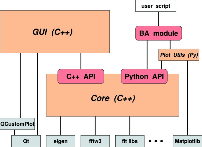
The BornAgain Python module (Section 4.2) is made from wrapper code that is distributed as part of the BornAgain source, but can be regenerated at any moment by running the open-source tool Swig. Besides this wrapper code, the BornAgain Python module also comprises some utility functions, written in Python, that facilitate and standardize use of the standard Python plotting library Matplotlib. The resulting code architecture is outlined in Fig. 1 ▸. The Core comprises about 60k lines of code, the GUI 90k.

Figure 1.

Overall code architecture (red: interfaces; orange: BornAgain components; gray: external dependencies; white: user code). The BornAgain Core can be controlled either from a GUI or from Python3 scripts. ‘BA module’ stands for the BornAgain Python module, which comprises a thin Python layer with plot utilities and the automatically generated Core wrapper.

3.4. Parallel computation  

To simulate a GISAS detector image, BornAgain runs a loop over all pixels. For each pixel, it computes the scattering cross section (Section 5.2) at a final wavevector given by the pixel’s coordinate. This algorithm lends itself to easy parallelization, since the computations at different are completely independent of each other.

BornAgain fully supports multi-threading. By default, all processor cores of the CPU are used. BornAgain can also be compiled with OpenMPI for multi-node computation on high-performance clusters.

3.5. Cross-platform support and build system  

BornAgain is actively supported for the three operating systems Linux, MacOS and Microsoft Windows, the last only in 64 bit versions. The download page provides installers for Mac and Windows. Installers for Linux may be added later; for the time being, Linux users have to compile from source.

Sources are distributed as a tarball. They come with input scripts for the meta-build system CMake. CMake generates makefiles for the Unix Make program, generator files for the Ninja build system, or project files for integrated development environments (IDEs), among them Microsoft Visual Studio. Thereby CMake generalizes the configure step of Unix-only source distributions, and enables native compilation under Microsoft Windows.

CMake searches for external library dependencies. These are currently the GNU scientific library for mathematical routines, including some fit algorithms, fftw3 for fast Fourier transform (Frigo & Johnson, 2005 ▸), libtiff for reading some detector images, some components of Boost, mostly for input/output processing, and Qt5 for the GUI. Some other libraries are distributed along with the BornAgain sources in a ThirdParty directory, mainly because they are not easily available in well-configured packages for all three supported platforms. These include Google tests, Minuit2 (a C++ rewrite of the Fortran fit library MINUIT, maintained by CERN and distributed within CERN’s ROOT library, but also available in a standalone version) and QCustomPlot. The library Eigen for vector and matrix algebra is included as a git submodule.

3.6. Tests  

The BornAgain sources contain different kinds of tests. They are all built and run using the CMake/CTest system.

Nearly 5000 EXPECT clauses in over 700 unit tests check specific functionality of over 150 classes. The unit test machinery relies on the Googletest C++ testing and mocking framework. GUI-related tests additionally depend on the introspection machinery of QtTest.

The functional tests, except a few special ones, are all regression tests. They run a full simulation on a specific instrument and sample model, and compare the result with a reference image that is also part of the BornAgain sources. These tests ensure that modifications of the code do not compromise the correctness and accuracy of simulation outcomes. They link back the current code to the earliest, still very simple versions of BornAgain, and to IsGISAXS. For speed reasons, the simulated detector has only 25 × 25 pixels.

The models and reference data of the Core regression tests are also used in Python and GUI functional tests. In the Python tests, C++ models are exported to Python, then a simulation is run under Python, which implicitly translates the model back to C++, and the final outcome is compared with the reference image. Similarly, in the GUI tests, C++ models are extended into GUI models, and simulations are run from the Born-AgainGUI library, without launching an actual GUI. In these ways, about 70 test cases can be run from C++, from Python and through the GUI machinery.

3.7. Online services  

The project web site https://www.bornagainproject.org/ provides detailed information on how to download, install and run BornAgain. It offers extensive tutorials, especially on how to set up various sample models. To produce these web pages, we use the static web site generator Hugo. All page sources are under version control. All code examples in the tutorials are also included in the BornAgain source distribution and are covered by tests, so that at any time all tests are guaranteed to work with the latest software release.

The web site provides links to the download location, to the git repository, to the issue tracker and to the subscription form of an announcements mailing list. For direct inquiries to the maintainers, a contact mail address is given. In the future, the API (application programming interface) reference, automatically generated by Doxygen, will be tightly integrated with usage examples and documentation of the implemented physics.

3.8. Outreach  

To meet user needs, we depend on feedback. The Born­Again team is in close contact with reflectometry scientists at our neutron source FRM II. To reach the GISAS community at large, we presented BornAgain in talks, posters and tutorials at numerous conferences in Europe, North America and East Asia. In 2013 we invited experienced users and developers of extant software to a workshop on GISAS data analysis.

In 2016 and 2018, we organized the first and second BornAgain School and User Meeting. Each time, more than 30 experimentalists attended. They were given an in-depth introduction to BornAgain, complemented by practical exercises. Advanced users presented their results. We intend to continue these meetings every two years.

4. User interfaces  

4.1. GUI  

BornAgain comes with a GUI. Based on the library Qt5, it has a native look and feel under all three supported operating systems (Section 3.5). It allows users to view experimental and simulated data, to set up and parameterize physical models, and to run fits.

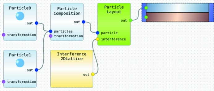
A graphical sample editor, vaguely inspired by the LabVIEW way of programming, allows users to assemble multilayer models by drag and drop. Model components like embedded particles or inter-particle correlation functions are represented by boxes that are connected by flexible lines to their parent components, as shown in Fig. 2 ▸.

Figure 2.

Representation of a sample in the GUI model editor. The hierarchical sample construction starts from the element in the upper-right corner, which just represents air above a substrate. The semi-infinite air layer is decorated with a particle layout, which combines a particle composition motif, composed of two spherical particles, with an inter-motif correlation function, namely a 2D lattice.

Simultaneously, the real-space structure of the sample, or any of its components, can be shown in an interactive 3D visualization (Fig. 3 ▸). This provides users with feedback as to whether the model, constructed in abstract terms in the sample editor, corresponds to their actual intentions. Moreover, a real-space representation can be helpful when communicating scientific results to audiences that are not familiar with the reciprocal-space thinking of scattering practitioners.

Figure 3.

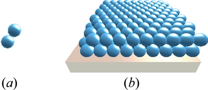
Real-space representation of the sample model of Fig. 2 ▸, a hexagonal bilayer on top of a substrate: (a) particle composition motif, (b) entire sample. In the GUI, these 3D views can be interactively rotated. The resulting GISAS pattern is shown in Fig. 11.

All model parameters can also be seen and set from a tree view. To explore their impact upon the simulated GISAS pattern, it is possible to modify parameter values with sliders. Unless the model is excessively computing intensive, the outcome view is kept up to date without noticeable delay.

All model and parameter choices made in an interactive GUI session can be stored in XML and can be reloaded in another GUI session. They can also be stored as a Python script, which can then be run from the command line, independently of the GUI. This helps users who reach the limits of GUI functionality to get started with using BornAgain from Python, since it is much easier to edit a given script than to write one from scratch.

4.2. Python interface  

The Python API enables users to run simulations and fits from the high-level programming language Python3. This can be done either in interactive sessions (possibly in a Jupyter notebook) or by executing a script. Once Python and BornAgain are installed on a computer, the simple command import bornagain as ba in a Python session or script is sufficient to make all the functionality of BornAgain available through function calls with the prefix ba.

The online documentation comprises numerous example scripts. For each script, the implemented model is explained and the obtained simulation result is shown. The same scripts are also contained in the BornAgain source tree. Typically, users will start from some example script and then gradually adapt it to their own needs. Another way to get started with scripting was previously mentioned in Section 4.1 – namely, build a model in the GUI and export it as a Python script.

Scripting is more versatile than the GUI and provides functionality that is not yet available in the GUI, or never will be. For instance, one can set up arbitrarily complicated combined and constrained fits. One can program the batch processing of huge data sets. One can react to a simulation or fit outcome through control clauses.

One can also extend the functionality of the BornAgain Core, for instance by adding particle form factors or correlation functions. Implementing such functionality in Python is less computing efficient than in C++, but in terms of development effort it can be an efficient way of rapid prototyping.

5. Simulated physics  

In this section we summarize the physical models implemented in BornAgain. After discussing geometric conventions, instrument models and detector coordinates (Section 5.1), we review the DWBA scattering cross section (Section 5.2) and add a word of caution about simulated peaks that are narrower than the detector bins (Section 5.3). We then discuss beam propagation in multilayers (Section 5.4) and the parameterization of refractive indices (Section 5.5). Finally, we present implemented models for sample inhomogeneities (Sections 5.6–5.13).

5.1. Geometrical conventions and detector models  

To describe GISAS geometry, we follow well-established conventions (Fig. 4 ▸). ‘Grazing incidence’ is understood relative to an average sample surface, always identified with the xy plane and called ‘horizontal’, no matter how it is oriented in laboratory space. The mean incident beam lies in the xz plane and originates from the quadrant x < 0, z > 0. The grazing angle is α; the azimuth angle φ is the deflection away from the xz plane.

Figure 4.

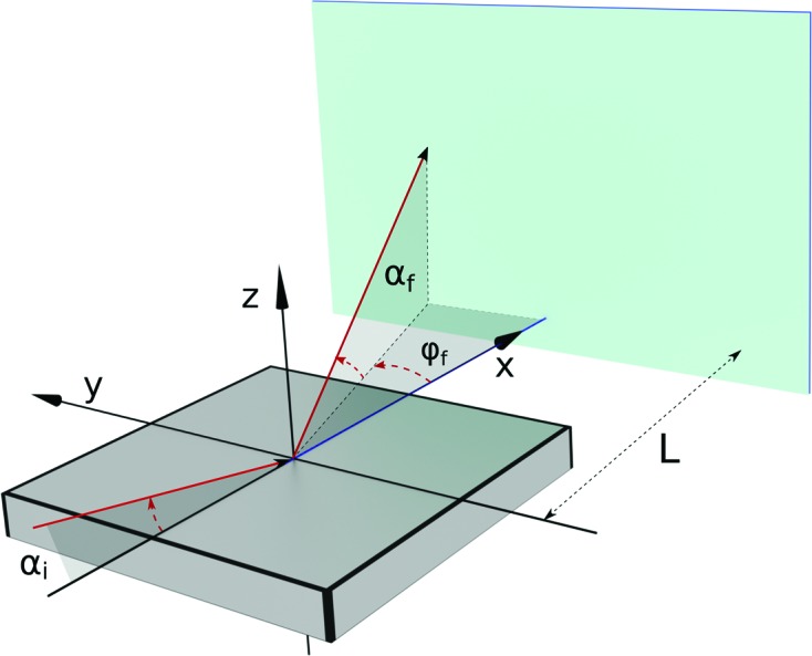
Geometric conventions in BornAgain. The average sample surface is the xy plane. The mean incident beam lies in the xz plane. The detector, at distance L from the origin, is perpendicular to .

Currently, instrument imperfections are modeled in reciprocal space only. Real-space characteristics like beam profile and finite sample surface will be added in future extensions for reflectometry (Section 8.1; compare Adlmann et al., 2018 ▸).

By default, BornAgain assumes a perfectly monochromatic and collimated incoming beam. This can be overwritten by explicit choices for the distributions of incoming wavelength, inclination and azimuth angle. So we admit , but the mean azimuth is .

Two detector geometries are supported: spherical and flat. A spherical detector is fairly unrealistic, but provides a means to visualize scattering patterns as functions of orthogonal coordinates and . The flat detector should be used when simulations are to be compared with experimental data from actual area detectors (e.g. Lehmann et al., 2011 ▸; Ponchut et al., 2011 ▸). By default, the detector lies in the yz plane, but can be tilted as specified by its normal vector n. In this way, we also support grazing-incidence wide-angle scattering.

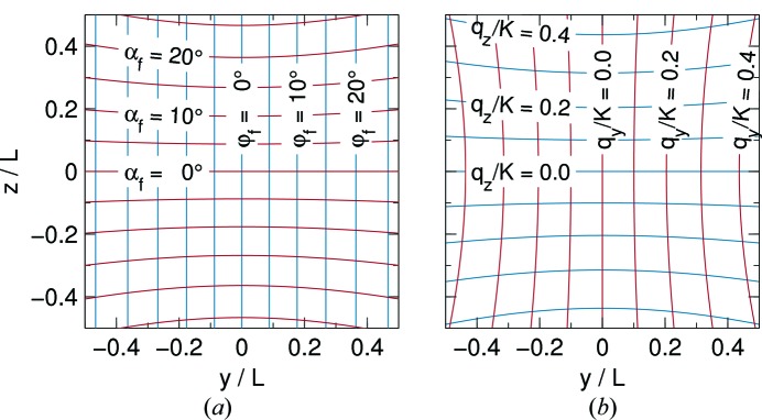
The natural pixel coordinates of the flat detector are y, z in units of mm. To facilitate physical interpretation, intensity maps can also be labeled with or , which are approximated proportional to y, z; no re-binning is done. As Fig. 5 ▸ illustrates, this is adequate only in the small-angle limit. Note also that is defined with respect to the direct (transmitted) beam, while the reflected terms in the GISAS cross section imply that some of the scattering actually occurs at .

Figure 5.

Scattering coordinate systems. Detector coordinates y, z are shown relative to the detector distance L. The red and blue curves are lines of constant (a) scattered beam angles , and (b) scattering vector components , the latter relative to the radiation wavenumber .

A finite detector resolution can be activated by choosing a Gaussian blur. The instrument model also offers a choice to add constant or Poisson noise to simulated detector images.

5.2. DWBA cross section  

The elastic scattering of neutrons and X-rays is governed by the wave equation

with the vacuum wave operator

at wavenumber K, and the potential (or scattering-length density, SLD)

The amplitude Ψ represents the scalar or spinorial neutron wavefunction, or the electric field, as applicable. The caret notation indicates, in the spinor case, a 2 × 2 matrix; the Pauli vector is composed of the three Pauli matrices . Fermi’s pseudopotential is used in the rescaled form:

The sum runs over all nuclei; is the bound scattering length (Sears, 1992 ▸). The magnetic moment μ of the neutron couples to the magnetic induction B (Mezei, 1986 ▸; Majkrzak et al., 2006 ▸),

where m is the neutron mass and ℏ is the reduced Planck constant. For the X-ray case, the simple form (2) depends on a few standard assumptions: non-conducting medium, hence no currents and no free charges, and no fast fluctuations of the permittivity ∊(r), except for jumps at layer interfaces.

In the DWBA, applied to layered samples (Dietrich & Wagner, 1984 ▸, 1985 ▸), the potential is split as

where depends only on depth z, while collects all fluctuations in x and y. The function can also be expressed through the refractive index:

With the distorted-wave operator , the wave equation (1) can be recast as

where the term on the right-hand side shall be treated as a small perturbation. In first order of the Rayleigh–Born expansion, the scattering cross section is

where are solutions of the unperturbed, homogeneous wave equation

subject to the boundary condition that they are plane waves at distant source and detector locations, respectively.

5.3. Caution about narrow structure-factor peaks  

At this point, a word of caution is in order. In BornAgain, by default the DWBA cross section is only evaluated at the centers of the detector bins. If the sample model results in a structure factor that varies substantially within one bin, then large discretization errors must be expected.

BornAgain currently has no mechanism to warn about this situation. It is entirely the responsibility of users to anticipate the possibility of narrow peaks and to take appropriate precautions. Since narrow peaks in q arise from long-range correlations in real space, one ought to be suspicious about thick layers, large embedded particles and especially crystalline order.

We recommend three ways to deal with narrow peaks. (i) Check whether the simulation outcome is stable under an increased or reduced number of bins.1 (ii) Run BornAgain in Monte Carlo mode to average for each bin over several q chosen at random. (iii) Extend the model to account for finite crystal size or finite coherence length, as discussed in Section 5.12.

5.4. Distorted waves for multilayers  

The boundary condition for the incident wave Ψ_i is determined by its vacuum wavevector k _i. The elastically scattered wave Ψ_f must be traced back from each single detector pixel; its vacuum wavevector k _f is given by the modulus and by the unit vector that points from the sample to the detector pixel.

Let us now designate Ψ either Ψ_i or Ψ_f. Solutions of (10) separate as

The wavevector component in the xy plane, , is constant. The vertical wave equation is

with

Its two solutions can be chosen to represent upwards and downwards traveling waves. So far BornAgain, as all extant software, only supports stepwise variations of .2 For the treatment of graded layers, see also Section 5.8.

Within layer j, the solution of (12) is simply

Standard continuity conditions at the layer interfaces yield linear couplings between the coefficients . Typically, the beam comes from above, so that in the top (air or vacuum) layer and in the bottom (substrate) layer. With these normalization and boundary conditions, the coefficients are fully determined.

The BornAgain Core and GUI provide an extra front end, DepthProbeSimulation, to compute the refracted and transmitted beam intensities as a function of depth and incident angle (Fig. 6 ▸). In preparing a GISAS experiment this allows users to choose the incident angle that maximizes the intensity available for scattering from within the sample.

Figure 6.

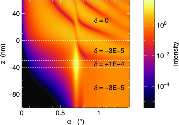
In depth-probe mode, BornAgain computes the refracted and transmitted beam intensity (squared amplitude) as a function of depth and incident angle. In this example, radiation with λ = 1 nm comes from vacuum (δ = 0) and enters at z = 0 a sample made of two layers on top of a substrate. Low-intensity bands show nodes of standing waves. An intensity maximum deep in the sample is found for α_i ≃ 0.7°.

In conclusion, the cross section (9) takes the DWBA form

with

For scalar wavefunctions, all this is standard and has been implemented in several extant codes (Section 2). New in BornAgain is the optional simulation of polarized neutron scattering, with a 2 × 2 matrix potential and spinor-valued coefficients A.

5.5. Materials parameterization  

Wave propagation through a multilayer (Section 5.4) is governed by the vertical wavenumber defined in (13). Re-parameterization in terms of wavenumber K and grazing angle α yields with

As expected, beam geometry only depends on the refractive index n. Since n is close to unity it is conveniently written as

The small real numbers δ and β are the primary means to specify a material in BornAgain [the sign of β comes from the quantum-mechanical convention chosen in (11) and (14)].

However, n depends on K. This is of no concern at monochromatic synchrotron sources, but can have noticeable consequences at neutron and laboratory X-ray instruments. To compensate for the explicit K ² dependence in (7), BornAgain supports an alternative specification of materials in terms of the SLD

If the need arises, we will also find ways to account for the dependence of on K, which is most pronounced near absorption resonances.

5.6. Rough interfaces  

Roughness breaks the translational symmetry of an interface and thereby causes diffuse scattering into off-specular directions. As the scattered intensity is lost from the reflected or transmitted beam, reflection and transmission coefficients no longer add up to 1. The reduction of reflected and transmitted intensity is described by the Névot–Croce factor (Névot & Croce, 1980 ▸). IsGISAXS supports this loss factor but not the diffuse scattering.

In BornAgain, diffuse scattering and beam attenuation are computed consistently. The roughness model is taken from the work of Schlomka et al. (1995 ▸). The height h is assumed to be a Gaussian random variable. The correlation function at in-plane distance R is

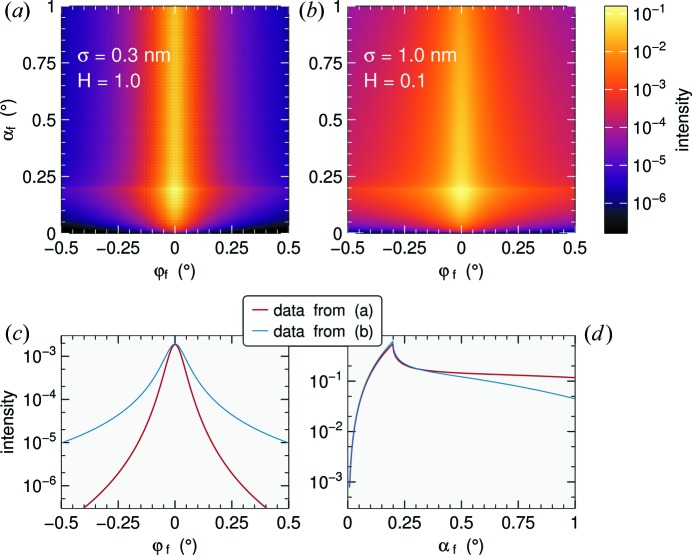
The user needs to specify the amplitude σ, the correlation length ξ and the Hurst parameter H. The latter is restricted to 0 < H ≤ 1. According to Schlomka et al. (1995 ▸), it defines the fractal box dimension D = 3 − H of the interface: the smaller H is, the more jagged is the interface. Typical simulation results are shown in Fig. 7 ▸.

Figure 7.

Diffuse scattering from rough interfaces. Collimated incoming beam with λ = 1 Å, α_i = 0.2°; substrate δ = 6 × 10⁻⁶, lateral correlation length ξ = 20 nm. (a) σ = 0.3 nm, H = 1; (b) σ = 1 nm, H = 0.1. In (c) and (d), the same data are integrated horizontally and vertically, respectively. The enhanced intensity below the critical angle α_c = 0.198°, known as the Yoneda peak, is due to scattering from the evanescent wave.

If there are two or more interfaces, then their height profiles may be correlated. Following again the work of Schlomka et al. (1995 ▸), this is specified through a vertical cross-correlation length that governs the correlations between two interfaces j and k,

5.7. Particle layout (incoherent sum)  

Many GISAS studies address droplets, islands, inclusions or holes of any size from nanometre to micrometre. As pioneered by IsGISAXS, all such inhomogeneities are described in BornAgain as particles that are embedded in a material layer.

In BornAgain, each layer can have one or more particle layouts. The total DWBA cross section is computed as an incoherent sum over these layouts l, weighted by their weight w_l,

This is essentially the local monodisperse approximation of IsGISAXS. Typically, different layouts stand for different spatial domains of the sample. Each layout contains particles of one or several given shapes (Section 5.8). Composite particles are also possible [Fig. 3 ▸(a), Section 5.9]. Within one layout, interference terms arise from inter-particle correlations (Section 5.11).

5.8. Particle form factors (also across layers)  

Particle shapes can be selected from a catalog of form factors. This catalog is visualized in the GUI by real-space pictures (Fig. 8 ▸); an exact description of the geometries and definitions of all parameters is given in the online documentation. IsGISAXS and FitGISAXS already supported quite a number of geometric forms. In BornAgain, they are all re-implemented and some more are added. The following innovations improve upon the legacy software.

Figure 8.

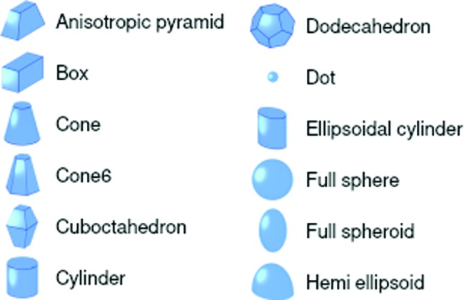
Part of the particle form-factor catalog in the GUI.

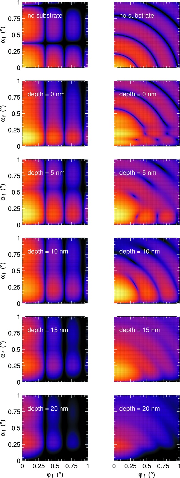
BornAgain fully supports absorbing media. Absorption causes a vertical damping of the incident and final wave, accounted for by an imaginary part of q_z. Since particles can be freely rotated, form-factor functions admit an arbitrary complex q argument. Particles are allowed to cross layer interfaces, as demonstrated in Fig. 9 ▸.

Figure 9.

Scattering from uncorrelated cylinders (left, R = H/2 = 10 nm) and spheres (right, R = 10 nm); δ = 6 × 10⁻⁴. Collimated incoming beam with λ = 1 Å, α_i = 0.2°. Top row: no substrate (Born approximation). The other rows: particles are immersed to the indicated depth in an absorbing substrate with δ = 6 × 10⁻⁶, β = 3 × 10⁻⁶. The common logarithmic intensity scale covers six decades and uses the same Matplotlib ‘inferno’ colors as all the other color maps.

Layers may consist of many sublayers to approximate a refractive index gradient. To support this, all supported particle shapes are equipped with form-factor functions for horizontal slices.3

Many of the supported particle shapes are polyhedra. Derivation of form factors by straightforward integration is cumbersome and yields expressions that contain removable singularities, causing numeric instabilities. We therefore preferred a generic solution (Wuttke, 2017 ▸), based on the Gauss and Stokes integral theorems, and parameterized in terms of edge topology and vertex coordinates. Near the singularities series expansions are used to avoid cancelation. To demonstrate the power of this method, we implemented the form factors of the regular dodecahedron and icosahedron. Other polyhedra can be supported as the need arises.

For large particles, keep in mind Section 5.3 on the evaluation of narrow peaks in a finite detector grid.

5.9. Particle composition  

A particle composition combines simple particles (with hard-coded form factors as described above) into a more complicated particle. This can be used to create arbitrary geometric shapes, to account for different SLDs (e.g. hard core and soft shell) and to construct a basis for a crystalline unit cell.

The resulting composed particle allows the same operations as simple particles: it can be further composed, rotated, translated and added to a layer’s particle layout. The scattering from a composed particle will correctly account for the coherent interference between its constituents.

5.10. Parameter distribution  

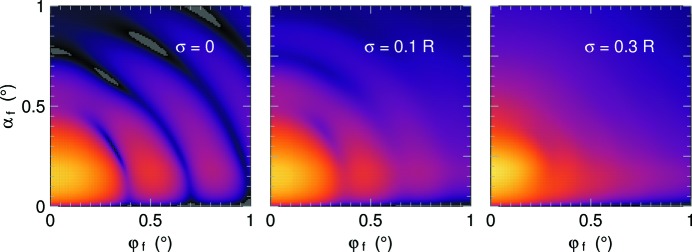
In many applications, the size and form parameters of nanoparticles have no uniform fixed values but follow some random distribution. GISAS patterns of such polydisperse systems are smoother than in the monodisperse limiting case; in particular, sharp minima are averaged out. This is exemplified in Fig. 10 ▸.

Figure 10.

Scattering from immersed spheres as in Fig. 9 ▸, at depth 10 nm. The spheres now have a Gaussian size distribution, with standard deviations σ from 0 to 0.3R. Logarithmic intensity scale, covering six decades, as before.

In BornAgain, stochastic distributions can be assigned to any particle geometry parameter, and to many other sample or instrument parameters, like interface roughness or incident wavelength. Available distributions include rectangular, trapezoid, Gaussian, Lorentzian and log-normal; for those with infinite support, lower and upper cutoffs can be set. To make one parameter proportional to another, one can impose a link.

If any parameter has a stochastic distribution, then the average DWBA cross section is computed from a configurable number of weighted equidistant parameter samples. In the concrete computation, however, a difference is made between particle geometry parameters and all other parameters. Sampled particles are all inserted in one and the same particle layout (Section 5.7) so that the DWBA cross section is obtained as a coherent sum. For all other sample and instrument parameters, the GISAS pattern is computed as an incoherent average over the parameter samples. This generalizes the parameter handling of IsGISAXS (Section 2.2.4 in Lazzari, 2006 ▸).

5.11. Particle correlations (interference functions)  

Particles, in the wide sense adopted here (Section 5.7), can aggregate in quite different structures, from complete disorder to crystalline lattices. Following IsGISAXS terminology, these models are implemented under the name interference function.

If no inter-particle correlation is specified, then BornAgain assumes perfect disorder, with structure factor , which of course is physical only for dilute systems. The dilute limit is safely reached when inter-particle distances are larger than , where Δq is the resolution width.

If excluded-volume interactions matter, then the next simplest model approximates particles as hard spheres, or hard discs in two dimensions. As GISAS is a surface technique, it is unsurprising that user demand so far has only been articulated for the 2D hard-disc model. Analytical solutions of the Percus–Yevick equation, however, seem to exist only for certain odd dimensions. Therefore we implemented the analytical approximation of Ripoll & Tejero (1995 ▸), which is in good accord with numeric results, though somewhat less so at packaging fractions above 0.5.

The next degree of ordering is represented by paracrystals (Hosemann, 1951 ▸). We implemented the radial and the 2D paracrystal exactly as in IsGISAXS (Lazzari, 2002 ▸, 2006 ▸). For the radial paracrystal, one can choose between the decoupling and the size-spacing correlation approximations.

5.12. Crystals, mesocrystals, superlattices  

Crystalline lattice structures in one, two and three dimensions can be specified in a straightforward way by supplying the one, two or three primitive vectors of the primitive Bravais lattice.4 Non-primitive bases are to be specified in the form of particle composition motifs. Fig. 11 ▸ shows the simulated GISAS pattern for the hexagonal bilayer introduced above in Figs. 2 ▸ and 3 ▸. Note that Bragg rods other than {00} are only observed for certain lattice orientations.

Figure 11.

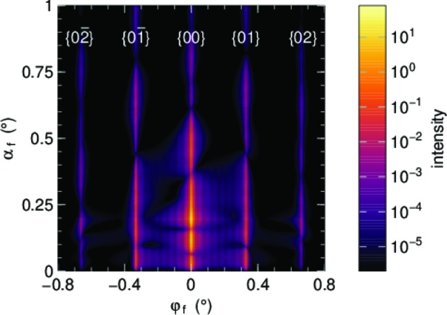
GISAS pattern of the sample model introduced above in Figs. 2 ▸ and 3 ▸: spherical nanoparticles (R = 10 nm, δ = 6 × 10⁻⁴), forming a hexagonal dense bilayer on top of a substrate (δ = 6 × 10⁻⁶), for a highly symmetric lattice orientation ({11} along x). The incident beam has λ = 1 Å, α_i = 0.2°. Bragg rods have been indexed manually. The finite horizontal extension of the rods is imposed through a decay function with correlation length 400 nm. The slight breaking of the mirror symmetry in φ_f is an artifact of our sample model with its rigid two-particle motif.

As anticipated in Section 5.3, the delta-shaped diffraction peaks of a perfect crystal are incompatible with our straightforward way of sampling the GISAS cross section at discrete q. Following IsGISAXS [Section 2.5.2 of Lazzari (2006 ▸)], BornAgain provides two ways to widen crystalline diffraction peaks: (i) the exact computation of finite size effects is most convincing for the modeling of well-known lithographic structures; (ii) in most other cases, finite-size effects are dominated by crystal defects and/or by the finite coherence length of the scattering apparatus. To model these imperfections, the delta functions are overridden ad hoc by finite peak shapes, called FTDecayFunctions because they can be construed, at least in a good approximation, as a Fourier transform of some decay of correlations in real space.

Mesocrystals are small crystalline aggregates of nanoparticles, typically formed by colloidal crystallization (e.g. Cölfen & Antonietti, 2005 ▸). If the size and distance of the mesocrystals are of a suitable scale, then GISAS is able to provide information on the size and outer shape of mesocrystals, and about their correlations. BornAgain supports mesocrystals in huge generality: to specify mesocrystal shape and inter-mesocrystal correlations, one can use the form factors and interference functions of Sections 5.8–5.11. For instance, one could model a hard-disc arrangement of cylindrical mesocrystals that consist of a face-centered cubic lattice of spherical nanoparticles. (Diffuse scattering from mesocrystals is not yet simulated, but this is expected to be implemented in a forthcoming release.)

To describe certain man-made surface structures, Born­Again also supports superlattices, which are 2D lattices of finite lattices.

Periodic gratings can be modeled as a 1D lattice of ripples or other elongated particles like pyramids or boxes. Of course only single scattering in the DWBA is simulated. Completely different computations are needed to account for higher-order dynamic scattering effects (Ashkar et al., 2010 ▸; Soltwisch et al., 2017 ▸).

5.13. Magnetism and neutron polarization  

The DWBA implementation of BornAgain fully supports polarized neutron propagation. With the exception of rough interfaces, all scattering models in BornAgain can be simulated for polarized neutrons. Specifically, this means that magnetic layers and magnetic particles can be simulated with a polarized neutron beam and optional polarization analysis at the detector. The underlying mechanism is essentially that of Kentzinger et al. (2008 ▸) and Toperverg (2015 ▸, and references 9, 10, 21, 45 therein). Other magnetic sample models will be implemented as requested by users. In particular, we expect interest in modeling domains in magnetic layers or magnetic roughness at layer interfaces.

By default, BornAgain assumes that the incoming beam is unpolarized and that there is no polarization analyzer after the sample. This is all one needs for X-rays and for nuclear scattering of neutrons. If there is magnetic neutron scattering, then BornAgain can be used to simulate all the functionality of a polarizing reflectometer, like MARIA at MLZ Garching (Mattauch et al., 2018 ▸). The incident polarization is to be specified as a Bloch vector, which allows one to encode any density matrix, but is more intuitive in that it allows one to directly read off the polarization direction and the extent of mixing. The polarization analyzer is specified in terms of orientation, efficiency and transmission.

An example of scattering by magnetized nanospheres is given in Fig. 12 ▸. The scattering cross section comprises nuclear, magnetic and interference terms. When polarizers are set for detection of spin-flip scattering, then nuclear scattering is suppressed; one only sees scattering from the magnetization component perpendicular to q (e.g. Chatterji, 2006 ▸). This explains the gap around φ_f = 0 in Fig. 12 ▸(b).

Figure 12.

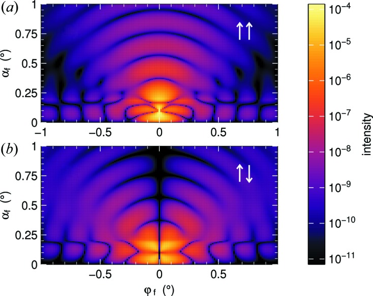
Polarized GISANS from vertically magnetized spherical nanoparticles (R = 30 nm, δ = 6 × 10⁻⁷, M = 400 kA m⁻¹) on top of a substrate (δ = 6 × 10⁻⁶). The incident beam has λ = 2 Å, α_i = 0.1°. The two simulations correspond to scattering (a) without and (b) with spin flip, assuming perfect vertical beam polarization and perfect polarization analysis.

6. Data processing and fitting  

6.1. Data import, visualization, masking and slicing  

BornAgain can read detector images from tiff files, from plain ASCII tables or from an internal ASCII storage format. For all other input, users are referred to the Python library FabIO (Knudsen et al., 2013 ▸) that can convert detector images from a huge variety of data formats used at X-ray instruments.

When the intensities supplied on input are all integers, and no error estimate is given, then it is presumed that the intensity D_i represents the number of independently scattered particles counted in pixel i, and the error estimate δD_i is taken from the Poisson standard deviation (D_i)^1/2.

Experimental scattering intensity histograms are plotted in the same way as simulated ones, i.e. as 2D color maps. In fitting mode, the GUI shows experimental and simulated data side by side, complemented by a difference image and a fit progress plot. Plots can be exported from the GUI as PNG graphics files. Under Python, the example scripts show how to plot data and simulations. From the Matplotlib pop-up window, plots can be exported to a variety of graphics formats, including PNG, TIFF and PDF.

To prepare data for 2D fitting it can be necessary to mask parts of the detector area, for instance those shadowed by the beamstop. In the GUI this can be done by drawing ellipses or polygonal contours. Data can also be projected into 1D histograms. This may be desired for conventional function plotting [as in Figs. 7 ▸(c) and 7 ▸(d)], and for the direct, sensitive comparison of data and fits.

6.2. Fit engines  

As with other BornAgain functionality, the fitting of parametric models to experimental data can also be steered from either the Python API or, to some extent, the GUI. To get started, one ties a model to a data set and chooses a residual function R_i, which can be the plain difference between data D_i and parametric model f_i(P), or the error-weighted difference , or the logarithm thereof. The default objective function is then the sum of squared residuals, .

At the core of the fitting procedure a minimizer algorithm searches for a minimum of χ² as a function of the parameter vector P. BornAgain comes with a choice of local and global minimizers, taken from several libraries, as specified in Section 3.5.

We wrote a wrapper that allows all minimizers to be called in the same way from the GUI or from Python scripts. The API of this wrapper closely follows that of the Python libraries bumps and lmfit. This allows users of the BornAgain Python API to choose either one of those Python minimizers, or one of the minimizers included in BornAgain, or even to concatenate different minimizers. Some of the minimizers allow or even require that parameters be restricted to finite intervals. Additional constraints, like coupling between parameters, can be imposed from the Python API.

6.3. Limitations of automatic fitting  

Automatic fitting of parametric models to experimental data is more difficult for GISAS than for most other scattering methods, and often is outright impossible. Many published GISAS analyses are only half-quantitative: they show qualitative agreement between the model and data, and extract some parameter values, but do not claim a ‘best fit’. We see two fundamental reasons for this: the high number of model parameters and the prevalence of systematic over stochastic uncertainties.

The high number of model parameters comes from the complexity of typical 2D samples. It is exacerbated when statistical distributions are needed to cope with fluctuations and imperfections caused by the intrinsic difficulties of thin-film preparation and alignment.

Typical GISAS patterns vary over decades in intensity, yet are much weaker than the reflected or transmitted direct beam. In such a situation, any inaccuracy in accounting for the strong signal components (e.g. the halos of the direct beam) will result in huge systematic uncertainty regarding the weak components. This then invalidates the objective function of a fit algorithm that depends on stochastic uncertainty estimates.

Since these difficulties overburden available automatisms, human users have to take back control. Still there is an important role for software, namely to provide versatile support for heuristic adjustments. BornAgain does this in particular through its masking and slicing facilities (Section 6.1).

7. Published usage  

As of July 2019, BornAgain has been used for data analysis in 19 published GISAXS and GISANS studies (not counting reviews, method papers and other publications that just mention BornAgain in passing). Four of these papers have been written in cooperation with one of us, some more acknowledge our help with BornAgain, some authors have attended a BornAgain school, but more than half of the published papers appeared without any personal involvement of ours: the authors just downloaded BornAgain and found their way to use it.

The studied samples represent the enormous breadth of modern surface science. They involve films of water (Gutfreund et al., 2016 ▸), alkane (Fontaine et al., 2018 ▸), lipid (Nylander et al., 2017 ▸), organic semiconductor (Zykov et al., 2017 ▸) and inorganic semiconductor (Highland et al., 2017 ▸; Singh et al., 2017 ▸); microgels (Kyrey et al., 2018 ▸) and microemulsions (Frielinghaus et al., 2017 ▸); templated (Li-Destri et al., 2016 ▸) and self-assembled polymer structures (Berezkin et al., 2018 ▸; Glavic et al., 2018 ▸; Xie et al., 2018 ▸); nanocolumns growing from vapor deposition (Haddad et al., 2016 ▸); Au nanoparticles during CO oxidation (Odarchenko et al., 2018 ▸); C₆₀ monolayer islands (Kowarik, 2017 ▸); magnetic nanoparticles (Ukleev et al., 2016 ▸, 2017 ▸) and magnetic films (Merkel et al., 2015 ▸; Glavic et al., 2018 ▸); lithographic gratings (Pflüger et al., 2019 ▸); and sputtered multilayers (Frielinghaus et al., 2017 ▸).

BornAgain is used in very different ways in these papers. Experiment and simulation are compared in the form of 2D detector images or of 1D projections. In most studies, the BornAgain model is manually tuned to reach good qualitative agreement with the experiment. Automatic fits are mainly done for 1D slices. Typically, the simulation yields sharper peaks than the experiment (Ukleev et al., 2016 ▸, 2017 ▸; Nylander et al., 2017 ▸). It remains to be seen whether this can be overcome by realistic modeling of instrument and/or sample imperfections. Pflüger et al. (2019 ▸) make the opposite choice: they do not even attempt to simulate a strong and nontrivial diffuse scattering; they fully concentrate on the sharp diffraction rings – which makes the accord of experiment and simulation no less impressive.

To demonstrate that a qualitative agreement between simulation and experiment is meaningful and informative, it can be helpful to present simulated detector images for modified models (Fontaine et al., 2018 ▸). Also, it can be very instructive to follow experiment and simulation through some parameter variation (Li-Destri et al., 2016 ▸; Singh et al., 2017 ▸; Berezkin et al., 2018 ▸).

8. Outlook  

To conclude, we briefly look beyond the current capabilities of BornAgain. Right now we are extending BornAgain towards reflectometry and off-specular scattering (Section 8.1). Application to ordinary small-angle scattering is possible though not actively promoted (Section 8.2). Finally, we mention alternatives to multi-parameter model fitting (Section 8.3).

8.1. Reflectometry and off-specular scattering  

As mentioned in Section 1, we are currently working on extending BornAgain to specular reflectometry and off-specular scattering, and will report in more detail on this in a sequel publication. Specular reflectometry is all about refracted and reflected intensities in a multilayer. The very same computations are needed by the DWBA (Section 5.4). Therefore, the sample model, the data structures and the core algorithms of BornAgain have long been ready for reflectometry simulations. Extra development effort is only needed to expose this functionality through convenient graphical and Python user interfaces. Similarly, off-specular scattering requires little more than an appropriate representation of yet another scan mode.

For the specular case, BornAgain will compete with quite a number of other data analysis programs: Aurore (Gerelli, 2016 ▸), GenX (Björck & Andersson, 2007 ▸), Motofit (Nelson, 2006 ▸, 2010 ▸), refnx (Nelson & Prescott, 2019 ▸), RasCAL (Hughes, 2014 ▸) and Refl1D (Kienzle et al., 2018 ▸). Against these, BornAgain stands out by its full support for neutron polarization, by its capability to derive scattering-length gradings from a rich and versatile particle decoration model, and not least by being institutionally supported. For users and instrument scientists of modern reflectometers, it will be convenient to have one and the same software cover all three scan modes. Ideally, this offer will encourage specular-only users to also explore the off-specular information, which a multi-detector captures anyway.

8.2. Small-angle scattering  

BornAgain, as with any GISAS code, can easily be adapted to fit and simulate ordinary small-angle scattering (SAS) by rotating the incoming beam and detector location. Since there will be almost no reflection from interfaces, the coefficients and in (14) can be set to zero, so that no sums over and must be computed in (15). This of course corresponds to replacing the DWBA by the ordinary Born approximation – an option which BornAgain anyhow offers for testing and teaching purposes.

However, there exist other institutionally supported codes for SAS analysis. In particular, within the European collaboration SINE2020 (see Section 1 and Acknowledgments) it was agreed to concentrate efforts on the software SasView (Doucet et al., 2018 ▸). Therefore, we do not promote Born­Again as a SAS software, and we do not offer user support for this application domain, except where BornAgain offers pertinent functionality that is lacking in SasView. This is especially the case for magnetic scattering, and for scattering from ordered nano- and mesoscale materials (Förster et al., 2011 ▸); to support research in this latter field, we extended our lattice models to three dimensions, replicating functionality of the soft-matter SAS software Scatter (Förster et al., 2010 ▸).

8.3. Beyond fitting  

As discussed in Section 6.3, model adjustment by automatic fitting becomes difficult or outright impossible if there are too many free parameters or if strong model components overshadow weak components and systematic uncertainties outweigh stochastic ones. One possible approach to this problem consists of reducing the task of data analysis by advanced data reduction, e.g. by ‘unwarping’ the four terms of the GISAS cross section (Liu & Yager, 2018 ▸). This may be worth a re-implementation within BornAgain. In reflectometry, the parameter-free determination of depth profiles by inversion of experimental curves has already been explored a number of times (de Haan et al., 1996 ▸; Majkrzak et al., 1997 ▸; Bushuev et al., 2002 ▸; Sutyrin & Prokhorov, 2006 ▸).

Another approach to cope with underdetermined multi-parameter models is machine learning. First applications to GISAS are promising (Wang et al., 2017 ▸; Liu et al., 2019 ▸). Well-trained deep neural networks can select models and deliver model parameters in microseconds, whereas manual fitting takes days at best. The precondition for this is a rich set of labeled training data. These data can be generated by running BornAgain on a powerful CPU cluster for a huge variety of models. We are currently exploring this idea in a pilot study (Van Herck et al., in preparation).

Funding Statement

This work was funded by Horizon 2020 grant 654000. Forschungszentrum Jülich grant NIK4#11. European Spallation Source ERIC grant NIK4#11.

References

- Abelès, F. (1950). J. Phys. Radium, 11, 307–309.
- Adlmann, F. A., Herbel, J., Korolkovas, A., Bliersbach, A., Toperverg, B., Van Herck, W., Pálsson, G. K., Kitchen, B. & Wolff, M. (2018). J. Phys. Condens. Matter, 30, 165901. [DOI] [PubMed]
- Ashkar, R., Stonaha, P., Washington, A. L., Shah, V. R., Fitzsimmons, M. R., Maranville, B., Majkrzak, C. F., Lee, W. T., Schaich, W. L. & Pynn, R. (2010). J. Appl. Cryst. 43, 455–465.
- Babonneau, D. (2010). J. Appl. Cryst. 43, 929–936.
- Berezkin, A. V., Jung, F., Posselt, D., Smilgies, D.-M. & Papadakis, C. M. (2018). Adv. Funct. Mater. 28, 1706226.
- Björck, M. & Andersson, G. (2007). J. Appl. Cryst. 40, 1174–1178.
- Bushuev, V. A., Lomov, A. A. & Sutyrin, A. G. (2002). Crystallogr. Rep. 47, 683–690.
- Chatterji, T. (2006). Neutron Scattering from Magnetic Materials. Amsterdam: Elsevier.
- Chourou, S. T., Sarje, A., Li, X. S., Chan, E. R. & Hexemer, A. (2013). J. Appl. Cryst. 46, 1781–1795.
- Cölfen, H. & Antonietti, M. (2005). Angew. Chem. Int. Ed. 44, 5576–5591. [DOI] [PubMed]
- Dietrich, S. & Wagner, H. (1984). Z. Phys. B Condens. Matter, 56, 207–215.
- Dietrich, S. & Wagner, H. (1985). Z. Phys. B Condens. Matter, 59, 35–42.
- Doucet, M., Cho, J. H., Alina, G., Bakker, J., Bouwman, W., Butler, P., Campbell, K., Gonzales, M., Heenan, R., Jackson, A., Juhas, P., King, S., Kienzle, P., Krzywon, J., Markvardsen, A., Nielsen, T., O’Driscoll, L., Potrzebowski, W., Ferraz Leal, R., Richter, T., Rozycko, P., Snow, T. & Washington, A. (2018). SasView Version 4.2, https://doi.org/10.5281/zenodo.1412041.
- Driessen, V. (2010). A Successful Git Branching Model, https://nvie.com/posts/a-successful-git-branching-model/.
- Fontaine, P., Bardin, L., Faure, M.-M., Filipe, E. J. M. & Goldmann, M. (2018). Nanoscale, 10, 2310–2316. [DOI] [PubMed]
- Förster, S., Apostol, L. & Bras, W. (2010). J. Appl. Cryst. 43, 639–646.
- Förster, S., Fischer, S., Zielske, K., Schellbach, C., Sztucki, M., Lindner, P. & Perlich, J. (2011). Adv. Colloid Interface Sci. 163, 53–83. [DOI] [PubMed]
- Frielinghaus, H., Gvaramia, M., Mangiapia, G., Jaksch, S., Ganeva, M., Koutsioubas, A., Mattauch, S., Ohl, M., Monkenbusch, M. & Holderer, O. (2017). Nucl. Instrum. Methods Phys. Res. A, 871, 72–76.
- Frigo, M. & Johnson, S. G. (2005). Proc. IEEE, 93, 216–231.
- Gentleman, R. C., Carey, V. J., Bates, D. M., Bolstad, B., Dettling, M., Dudoit, S., Ellis, B., Gautier, L., Ge, Y., Gentry, J., Hornik, K., Hothorn, T., Huber, W., Iacus, S., Irizarry, R., Leisch, F., Li, C., Maechler, M., Rossini, A. J., Sawitzki, G., Smith, C., Smyth, G., Tierney, L., Yang, J. Y. H. & Zhang, J. (2004). Genome Biol. 5, R80. [DOI] [PMC free article] [PubMed]
- Gerelli, Y. (2016). J. Appl. Cryst. 49, 330–339.
- Glavic, A., Summers, B., Dahal, A., Kline, J., Van Herck, W., Sukhov, A., Ernst, A. & Singh, D. K. (2018). Adv. Sci. 5, 1700856. [DOI] [PMC free article] [PubMed]
- Glinz, M. (2007). 15th IEEE International Requirements Engineering Conference, https://doi.org/10.1109/RE.2007.45.
- Gutfreund, P., Maccarini, M., Dennison, A. J. C. & Wolff, M. (2016). Langmuir, 32, 9091–9096. [DOI] [PubMed]
- Haan, V. O. de, van Well, A. A., Sacks, P. E., Adenwalla, S. & Felcher, G. P. (1996). Physica B, 221, 524–532.
- Haddad, K., Abokifa, A., Kavadiya, S., Chadha, T. S., Shetty, P., Wang, Y., Fortner, J. & Biswas, P. (2016). CrystEngComm, 18, 7544–7553.
- Hexemer, A. & Müller-Buschbaum, P. (2015). IUCrJ, 2, 106–125. [DOI] [PMC free article] [PubMed]
- Highland, M. J., Hruszkewycz, S. O., Fong, D. D., Thompson, C., Fuoss, P. H., Calvo-Almazan, I., Maddali, S., Ulvestad, A., Nazaretski, E., Huang, X., Yan, H., Chu, Y. S., Zhou, H., Baldo, P. M. & Eastman, J. A. (2017). Appl. Phys. Lett. 111, 161602.
- Hinsen, K. (2016). Winnower, 5, e146857.76572.
- Hosemann, R. (1951). Acta Cryst. 4, 520–530.
- Hughes, A. (2014). RasCAL, https://sourceforge.net/projects/rscl/.
- Ince, D. C., Hatton, K. & Graham-Cumming, J. (2012). Nature, 482, 485–488. [DOI] [PubMed]
- Jaksch, S., Gutberlet, T. & Müller-Buschbaum, P. (2019). Curr. Opin. Colloid Interface Sci. 42, 73–86.
- Jiménez, R. C., Kuzak, M., Alhamdoosh, M., Barker, M., Batut, B., Borg, M., Capella-Gutierrez, S., Chue Hong, N., Cook, M., Corpas, M., Flannery, M., Garcia, L., Gelpí, J. Ll., Gladman, S., Goble, C., González Ferreiro, M., Gonzalez-Beltran, A., Griffin, P. C., Grüning, B., Hagberg, J., Holub, P., Hooft, R., Ison, J., Katz, D. S., Leskošek, B., López Gómez, F., Oliveira, L. J., Mellor, D., Mosbergen, R., Mulder, N., Perez-Riverol, Y., Pergl, R., Pichler, H., Pope, B., Sanz, F., Schneider, M. V., Stodden, V., Suchecki, R., Svobodová Vařeková, R., Talvik, H. A., Todorov, I., Treloar, A., Tyagi, S., van Gompel, M., Vaughan, D., Via, A., Wang, X., Watson-Haigh, N. S. & Crouch, S. (2017). F1000Res, 6, 876.
- Joppa, L. N., McInerny, G., Harper, R., Salido, L., Takeda, K., O’Hara, K., Gavaghan, D. & Emmott, S. (2013). Science, 340, 814–815. [DOI] [PubMed]
- Kentzinger, E., Rucker, U., Toperverg, B., Ott, F. & Bruckel, T. (2008). Phys. Rev. B, 77, 104455.
- Kienzle, P. A., Krycka, J., Patel, N. & Sahin, I. (2018). Refl1D, https://github.com/reflectometry/refl1d.
- Knudsen, E. B., Sørensen, H. O., Wright, J. P., Goret, G. & Kieffer, J. (2013). J. Appl. Cryst. 46, 537–539.
- Kowarik, S. (2017). J. Phys. Condens. Matter, 29, 043003. [DOI] [PubMed]
- Kyrey, T., Ganeva, M., Gawlitza, K., Witte, J., von Klitzing, R., Soltwedel, O., Di, Z., Wellert, S. & Holderer, O. (2018). Physica B, 551, 172–178.
- Lazzari, R. (2002). J. Appl. Cryst. 35, 406–421.
- Lazzari, R. (2006). IsGISAXS, http://www.insp.jussieu.fr/oxydes/IsGISAXS/isgisaxs.htm.
- Lehmann, E. H., Tremsin, A., Grünzweig, C., Johnson, I., Boillat, P. & Josic, L. (2011). J. Instrum. 6, C01050.
- Li-Destri, G., Tummino, A., Malfatti Gasperini, A. A., Parellada Monreal, L., Messina, G. M. L., Spampinato, V., Ceccone, G. & Konovalov, O. (2016). RSC Adv. 6, 9175–9179.
- Liu, J. & Yager, K. G. (2018). IUCrJ, 5, 737–752. [DOI] [PMC free article] [PubMed]
- Liu, S., Melton, C. N., Venkatakrishnan, S., Pandolfi, R. J., Freychet, G., Kumar, D., Tang, H., Hexemer, A. & Ushizima, D. M. (2019). MRS Commun 9, 586–592.
- Majkrzak, C. F., Berk, N. F., Dura, J., Satija, S. K., Karim, A., Pedulla, J. & Deslattes, R. D. (1997). Physica B, 241–243, 1101–1103.
- Majkrzak, C. F., O’Donovan, K. V. & Berk, N. F. (2006). Neutron Scattering from Magnetic Materials, edited by T. Chatterji, ch. 9. Amsterdam: Elsevier.
- Markvardsen, A. (2017). Report on Guidelines and Standards for Data Treatment software, https://sine2020.eu/news-and-media/standard-and-guidelines-for-data-treatment-software-defined-as-first-deliverable-in-wp10.html.
- Mattauch, S., Koutsioubas, A., Rücker, U., Korolkov, D., Fracassi, V., Daemen, J., Schmitz, R., Bussmann, K., Suxdorf, F., Wagener, M., Kämmerling, P., Kleines, H., Fleischhauer-Fuß, L., Bednareck, M., Ossoviy, V., Nebel, A., Stronciwilk, P., Staringer, S., Gödel, M., Richter, A., Kusche, H., Kohnke, T., Ioffe, A., Babcock, E., Salhi, Z. & Bruckel, T. (2018). J. Appl. Cryst. 51, 646–654. [DOI] [PMC free article] [PubMed]
- Merkel, D. G., Bessas, D., Zolnai, Z., Ruffer, R., Chumakov, A. I., Paddubrouskaya, H., Van Haesendonck, C., Nagy, N., Tóth, A. L. & Deak, A. (2015). Nanoscale, 7, 12878–12887. [DOI] [PubMed]
- Meyer, B. (2014). Agile!: The Good, the Hype and the Ugly. Cham: Springer.
- Mezei, F. (1986). Physica B+C, 137, 295–308.
- Müller-Buschbaum, P. (2013). Polym. J. 45, 34–42.
- Nelson, A. (2006). J. Appl. Cryst. 39, 273–276.
- Nelson, A. (2010). J. Phys. Conf. Ser. 251, 012094.
- Nelson, A. R. J. & Prescott, S. W. (2019). J. Appl. Cryst. 52, 193–200. [DOI] [PMC free article] [PubMed]
- Névot, L. & Croce, P. (1980). Rev. Phys. Appl. (Paris), 15, 761–779.
- Nylander, T., Soltwedel, O., Ganeva, M., Hirst, C., Holdaway, J., Arteta, M., Wadsäter, M., Barauskas, J., Frielinghaus, H. & Holderer, O. (2017). J. Phys. Chem. B, 121, 2705–2711. [DOI] [PubMed]
- Nyman, L. & Lindman, J. (2013). Technol. Innov. Manag. Rev. 3, 7–12.
- Odarchenko, Y., Martin, D. J., Arnold, T. & Beale, A. M. (2018). Faraday Discuss. 208, 243–254. [DOI] [PubMed]
- Parnas, D. L. & Clements, P. C. (1986). IEEE T. Software Eng. SE-12, 251–257.
- Paul, A. (2012). Pramana J. Phys. 78, 1–58.
- Peng, R. D. (2011). Science, 334, 1226–1227. [DOI] [PMC free article] [PubMed]
- Pflüger, M., Soltwisch, V., Xavier, J., Probst, J., Scholze, F., Becker, C. & Krumrey, M. (2019). J. Appl. Cryst. 52, 322–331.
- Ponchut, C., Rigal, J. M., Clément, J., Papillon, E., Homs, A. & Petitdemange, S. (2011). J. Instrum. 6, C01069.
- Prlić, A. & Procter, J. B. (2012). PLoS Comput. Biol. 8, e1002802. [DOI] [PMC free article] [PubMed]
- Renaud, G., Lazzari, R. & Leroy, F. (2009). Surf. Sci. Rep. 64, 255–380.
- Ripoll, M. S. & Tejero, C. F. (1995). Mol. Phys. 85, 423–428.
- Sarje, A., Kumar, D., Venkatakrishnan, S., Li, X., Hexemer, A., Chourou, S. & Chan, E. (2016). HipGISAXS, https://hipgisaxs.github.io/.
- Schlomka, J.-P., Tolan, M., Schwalowsky, L., Seeck, O. H., Stettner, J. & Press, W. (1995). Phys. Rev. B, 51, 2311–2321. [DOI] [PubMed]
- Schwartzkopf, M., Buffet, A., Korstgens, V., Metwalli, E., Schlage, K., Benecke, G., Perlich, J., Rawolle, M., Rothkirch, A., Heidmann, B., Herzog, G., Muller-Buschbaum, P., Rohlsberger, R., Gehrke, R., Stribeck, N. & Roth, S. V. (2013). Nanoscale, 5, 5053–5062. [DOI] [PubMed]
- Schwartzkopf, M., Santoro, G., Brett, C. J., Rothkirch, A., Polonskyi, O., Hinz, A., Metwalli, E., Yao, Y., Strunskus, T., Faupel, F., Müller-Buschbaum, P. & Roth, S. V. (2015). Appl. Mater. Interfaces, 7, 13547–13556. [DOI] [PubMed]
- Sears, V. P. (1992). Neutron News, 3(3), 26–37.
- Singh, A., Schipmann, S., Mathur, A., Pal, D., Sengupta, A., Klemradt, U. & Chattopadhyay, S. (2017). Appl. Surf. Sci. 414, 114–123.
- Soltwisch, V., Fernández Herrero, A., Pflüger, M., Haase, A., Probst, J., Laubis, C., Krumrey, M. & Scholze, F. (2017). J. Appl. Cryst. 50, 1524–1532.
- Sutyrin, A. G. & Prokhorov, D. Y. (2006). Crystallogr. Rep. 51, 570–576.
- Tate, M. P., Urade, V. N., Kowalski, J. D., Wei, T. C., Hamilton, B. D., Eggiman, B. W. & Hillhouse, H. W. (2006). J. Phys. Chem. B, 110, 9882–9892. [DOI] [PubMed]
- Toperverg, B. P. (2015). Phys. Met. Metallogr. 116, 1337–1375.
- Ukleev, V., Khassanov, A., Snigireva, I., Konovalov, O., Dudnik, M., Dubitskiy, I. & Vorobiev, A. (2017). Mater. Chem. Phys. 202, 31–39.
- Ukleev, V., Khassanov, A., Snigireva, I., Konovalov, O. & Vorobiev, A. (2016). Thin Solid Films, 616, 43–47.
- Vallee, O. & Soares, M. (2010). Airy Functions and Applications to Physics. New Jersey: Imperial College Press.
- Venkatakrishnan, S. V., Donatelli, J., Kumar, D., Sarje, A., Sinha, S. K., Li, X. S. & Hexemer, A. (2016). J. Appl. Cryst. 49, 1876–1884.
- Wang, B., Yager, K., Yu, D. & Hoai, M. (2017). IEEE Winter Conference on Applications of Computer Vision (WACV). https://doi.org/10.1109/WACV.2017.83.
- Willinsky, J. (2005). First Monday, 10, 8.
- Wilson, G., Aruliah, D. A., Brown, C. T., Chue Hong, N. P., Davis, M., Guy, R. T., Haddock, S. H., Huff, K. D., Mitchell, I. M., Plumbley, M. D., Waugh, B., White, E. P. & Wilson, P. (2014). PLoS Biol. 12, e1001745. [DOI] [PMC free article] [PubMed]
- Wuttke, J. (2017). arXiv:1703.00255.
- Xie, C., Heumüller, T., Gruber, W., Tang, X., Classen, A., Schuldes, I., Bidwell, M., Späth, A., Fink, R. H., Unruh, T., McCulloch, I., Li, N. & Brabec, C. J. (2018). Nat. Commun. 9, 5335. [DOI] [PMC free article] [PubMed]
- Zykov, A., Bommel, S., Wolf, C., Pithan, L., Weber, C., Beyer, P., Santoro, G., Rabe, J. P. & Kowarik, S. (2017). J. Chem. Phys. 146, 052803. [DOI] [PubMed]