Figure 1 Theory Meets Figure 2 Experiments in the Study of Gene Expression

Abstract

It is tempting to believe that we now own the genome. The ability to read and rewrite it at will has ushered in a stunning period in the history of science. Nonetheless, there is an Achilles’ heel exposed by all of the genomic data that has accrued: We still do not know how to interpret them. Many genes are subject to sophisticated programs of transcriptional regulation, mediated by DNA sequences that harbor binding sites for transcription factors, which can up- or down-regulate gene expression depending upon environmental conditions. This gives rise to an input-output function describing how the level of expression depends upon the parameters of the regulated gene—for instance, on the number and type of binding sites in its regulatory sequence. In recent years, the ability to make precision measurements of expression, coupled with the ability to make increasingly sophisticated theoretical predictions, has enabled an explicit dialogue between theory and experiment that holds the promise of covering this genomic Achilles’ heel. The goal is to reach a predictive understanding of transcriptional regulation that makes it possible to calculate gene expression levels from DNA regulatory sequence. This review focuses on the canonical simple repression motif to ask how well the models that have been used to characterize it actually work. We consider a hierarchy of increasingly sophisticated experiments in which the minimal parameter set learned at one level is applied to make quantitative predictions at the next. We show that these careful quantitative dissections provide a template for a predictive understanding of the many more complex regulatory arrangements found across all domains of life.

Hic rhodus, hic salta.

–Aesop’s Fables

1. INTRODUCTION

The study of transcriptional regulation is one of the centerpieces of modern biology. It was set in motion by the revolutionary work of Jacob and Monod in the postwar era, which culminated in their elucidating the concept of transcriptional regulation in the early 1960s (42, 65, 66), and it has continued apace ever since. Based on their study of the lac operon and regulation of the life cycle of bacterial viruses, Jacob and Monod hypothesized that transcription was controlled using a mechanism sometimes known as the repressor-operator model, in which repressive factors bind to promoters at sites called operators to prevent activation of genes. Here, we refer to this regulatory architecture as the simple repression motif.

Jacob and Monod suspected that there would be a universal mechanism for transcriptional regulation that followed the strictures of the repressor-operator model; indeed, simple repression, defined diagrammatically in Figure 1a, has since been shown to have widespread applicability, as seen in Figure 1b. However, transcriptional reality is—as is usually the case in biology—far more complicated (13), and, as Figure 1 reveals, many genes are in fact subject to both negative and positive regulation. Ironically, the genetic circuit used by Monod to formulate the repressor-operator model—the lac operon shown in Figure 2—is itself subject to positive regulation, which shows the repressor-operator model to be incomplete (27, 117).

Figure 1.

The distribution of regulatory architectures in Escherichia coli. (a) Several of the simplest regulatory architectures are shown, featuring activator and repressor binding sites. We adopt the notation (m, n) to characterize these architectures, where the first number m tells us how many activator binding sites there are for our gene of interest, and the second number n tells us how many repressor binding sites are controlling that same gene. Within this notation, a (0, 0) architecture is unregulated, a (1, 0) architecture is a simple activation motif, and a (0, 1) architecture is a simple repression motif and is the central focus of the present article. (b) Relative probability of different classes of regulatory architecture for those genes that have been annotated in E. coli (30, 89). For transcription factors that can act as both activators and repressors, we consider their specific mode of action in the context of each regulatory architecture. For example, if a transcription factor binds to a single site near a promoter and acts as an activator, we consider it to fall within the (1, 0) nomenclature even if this same protein can act as a repressor on other regulatory units.

Figure 2.

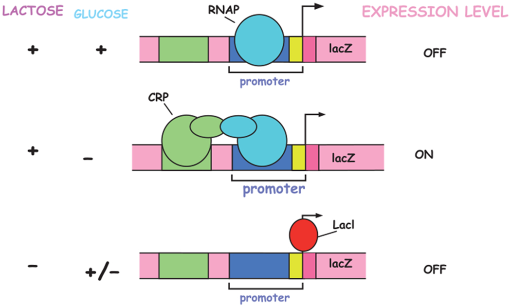
The high school lac operon. The classic story of how bacteria utilize lactose rather than glucose as a carbon source is the canonical example used to teach the concept of genetic regulation. The figure shows that only when lactose is present and glucose is absent will the gene for the enzyme used to digest lactose be turned on. The activator is shown in green, the repressor is shown in red, and RNA polymerase is depicted in blue.

The lac operon is one of the canonical case studies learned by high school and college students alike when they are first introduced to the logic of gene regulation in modern molecular and cellular biology (2, 68). Figure 2 shows in cartoon form how the gene that encodes the enzyme for digesting lactose is activated only when lactose is present and glucose is absent. This textbook case of transcriptional regulation has been studied to death, but how well do we really understand it? The sketch in Figure 2 is a broad-brush view of transcriptional control at the lac operon, but it gives us no sense of how the level of gene expression is affected by, for example, changing the copy numbers of the LacI and CRP transcription factors, changing the positioning of the operator, or titrating the relative concentrations of glucose and lactose. We argue that achieving real understanding of this system requires that we be capable of making precise and quantitative predictions about its regulatory response as a function of all these parameters, and then that we be able to confirm these predictions experimentally.

How could we achieve this mastery? First, we would need theoretical models able to provide quantitative predictions that can be tested with careful experiments. Importantly, both the predictions and the experiments themselves would need to access the same underlying knobs to control the level of gene expression. Second, we would need to start with the simplest of regulatory architectures. If we are unable to understand the most basic regulatory kernel, then we have no hope of doing so for more complex regulatory circuits. Third, to dissect more subtle features of a regulatory circuit—for instance, to understand how expression noise depends on changing parameters—we must be able to use quantitative information gleaned from one type of experiment to formulate further predictions that are tested in subsequent experiments of a different type. Therefore, we would need to conduct all these experiments in the same system and under standardized conditions.

This review summarizes such an approach, which we have taken in our own laboratory over the past decade. We discuss how, working with a set of specifically designed synthetic constructs and challenging theoretical models with experiments, we have been able to tackle increasingly subtle behaviors of the simple repression architecture in Escherichia coli. The strategy that we have taken results in a pyramidal structure, as shown in Figure 3, in which parameters inferred at one level are used to make quantitative predictions about gene expression behavior in successive, more sophisticated experiments.

Figure 3.

The simple repression pyramid. A progression of different experiments makes it possible to assess increasingly subtle regulatory effects for the simple repression motif. Parameters inferred from lower levels in the pyramid are used in the analysis of the experiments at the next level. The repressor (and its binding site) is shown in red, RNA polymerase (and its binding site) is shown in blue, and inducer is shown in green.

At the foundation of the simple repression pyramid are experiments to determine how gene expression responds to changes in operator strength and repressor copy number. With this information in hand, we can then consider the entire distribution of expression levels among a population of cells, as opposed to simply the average expression. At the next level in the hierarchy, we address a number of subtle and beautiful effects that arise when there is more than one copy of our gene of interest or competing binding sites for the repressor elsewhere on the genome (or on plasmids). This repressor titration effect provides a very stringent test of our understanding of the simple repression motif. Of course, much of gene expression is dictated by the presence of environmental signals, and the next level in the simple repression pyramid is to ensure that these same kinds of predictive models can describe induction of transcription. Furthermore, changes in the environment such as media quality or growth temperature certainly have an effect on the bacterial doubling rate. The next challenge is then to retain predictive power by describing how these different conditions affect the magnitude of parameters that are the basis of these models, such as repressor copy number and binding energy. Finally, evolution of transcription acts at the level of both transcription factor binding sites and the transcription factors that bind to them. Ultimately, the simple repression pyramid will be topped off by learning the rules that relate transcriptional regulation to fitness (7, 35, 54, 60). At every level in the pyramid, we demand that the parameters be self-consistent. That is, regardless of how our experiments are done or which new question we ask, the same minimal parameter set is used without recourse to new fits for each new experiment.

Note that this article is not a review of a field; rather, it is a review of a concept, in which one minimal parameter set is asked to describe all measurements on a particular realization of the simple repression motif. This objective is not served by an approach in which different measurements are taken from disparate sources on different strains under different conditions. We focus instead on measurements made using the same strains under the same growth conditions throughout, and this renders the discussion highly self-referential. But everything that we have done was enabled by beautiful work that has come before and inspired by wonderful experiments since; we point the reader toward as much of this literature as possible.

The goal of this review is to address whether, for simple repression, we have reached a self-consistent theoretical picture that stands up to careful experimental scrutiny. After an overview of regulatory architectures in E. coli, and the simple repression motif in particular, we describe our systematic effort to make the strains, tune the relevant knobs, and make the high-precision measurements that enable us to test theoretical predictions about how the simple repression architecture behaves. In the following sections, we then address the key critiques of the theoretical framework, before stepping back to discuss what our results entail for future efforts in understanding gene regulation. We argue that we have achieved significant success using this hierarchical approach and that it provides hope for understanding other, more complex, gene regulatory circuits. Indeed, the great work done by others in lac (52, 90, 110), MarA (3, 62), GalR (96, 97, 105), Lambda (23, 24, 79, 116), and AraC (93) lends itself to providing the fundamental stepping stones for building other transcriptional pyramids.

2. THE REGULATORY LANDSCAPE IN ESCHERICHIA COLI AND THE UBIQUITOUS SIMPLE REPRESSION ARCHITECTURE

Despite the dominance of E. coli as a model system for studying gene regulation, we remarkably have little or no idea how most of its genes are controlled. As Figure 4 demonstrates, for the majority of genes, we do not know the identity of the transcription factors that turn them on/off, where the binding motifs for those transcription factors are, or what the regulatory logic is (at the most basic level, whether they are controlled by repressors, activators, or a combination of both). Figure 1 provides an incomplete, but state-of-the-art picture of our current knowledge of the regulatory landscape by showing the distribution of different architecture types in E. coli. Shortly after the elucidation of the repressor-operator model [the (0, 1) motif] that introduced the simple repression architecture that we focus on here, the idea of activation as a regulatory mechanism also took root. But as we see in Figure 1b, at the time of this writing, most genes in E. coli are annotated as unregulated. This sounds counterintuitive, but for many genes it likely reflects ignorance of the binding motifs and regulators, as opposed to actual lack of any regulation. Simple repression (along with simple activation) comes in as the next most prevalent architecture, and we now turn our attention there.

Figure 4.

Regulatory ignorance in Escherichia coli. The central figure, which schematizes the E. coli genome, shows the fraction of the operons for which we know nothing about how they are regulated. The left panels show examples of the knowledge of regulatory architectures required to unleash the kind of theory–experiment dialogue described here. The right panel shows the more common situation, which is complete regulatory ignorance.

Simple repression is a common regulatory motif in E. coli (89), but we know little of the general principles by which it is used. To tackle this, we used annotated regulatory information from RegulonDB (30) to survey 156 promoters with a simple repression architecture, controlled by 50 different transcription factors. We first wanted to know how the concentrations of these regulators change under different growth conditions, and how this relates to their probability of binding to the promoters in question

To characterize each promoter, we used published data that quantified protein abundance across the bacterial proteome under various growth conditions using either ribosomal profiling or mass spectrometry (58, 95). Figure 5a shows the distribution of repressor and activator copy numbers genome wide, while Figure 5b shows the copy numbers for just those repressors that target the (0, 1) architectures in which we are interested. The transcription factors vary in copy number from 0 to about 10,000 per cell. Of the repressors, just over half of them bind 10 or fewer binding sites, while some target over 100 binding sites across the genome (Figure 5e). Given the wide range in repressor copy number, we wondered whether it related to the number of target binding sites that exist for each of these repressors in the genome. Indeed, when we calculated the ratio between protein copy number and number of target binding sites for each transcription factor (as indicated by the dashed lines in Figure 5b), we found a median ratio of about 15 transcription factor copies per binding site. The majority of the transcription factors (about 80%) have no more than 100 copies per binding site. Given that the number of transcription factors per binding site is on the order of 10–100, we can infer that their typical effective binding constants (defined in detail below) are in the 10–100 nM range, since 1 copy of a protein per bacterial cell corresponds to a concentration of roughly 1 nM.

Figure 5.

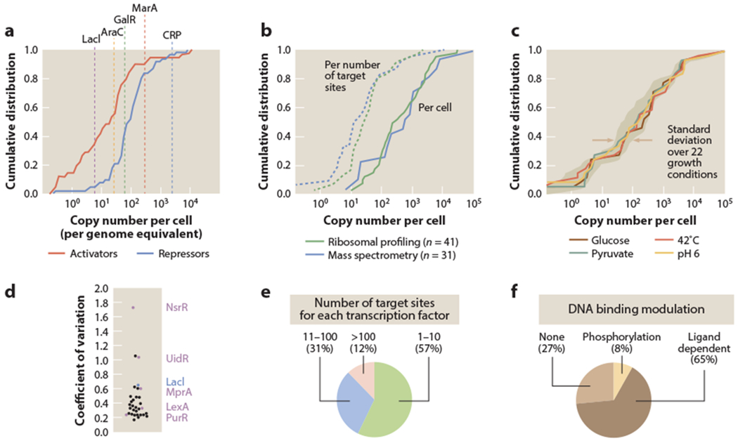
Summary of transcription factors that target the (0, 1) simple repression architecture. (a) Transcription factor copy numbers in Escherichia coli (58). The cumulative distribution of transcription factor copy numbers indicates that activator copy numbers are generally lower than repressor copy numbers. Roughly half of the activators have copy number less than 10, while roughly half of all repressors have copy number less than 100. Several representative examples of well known transcription factors are shown for reference. (b) Cumulative distributions are shown for transcription factors that target the (0, 1) simple repression architecture. Data are shown from measurements using ribosomal profiling [41 of the 50 identified repressors were measured in MOPS minimal media with 0.2% glucose (58)] and mass spectrometry [31 of the 50 identified repressors were measured in M9 minimal media with 0.5% glucose (95)]. (c) The variability in cumulative distribution is shown for the 31 transcription factors regulating the (0, 1) architecture measured across 22 different growth conditions, using mass spectrometry. The shaded region represents the 95th percentile region in cumulative distributions across growth conditions, with the distributions for four growth conditions shown explicitly. (d) Coefficient of variation for copy numbers of transcription factors regulating the (0, 1) architecture across the 22 different growth conditions, measured by mass spectrometry. Several examples are identified along with LacI, and the complete list is summarized in Table 1. (e) Number of target binding sites for each of the transcription factors that target a (0, 1) architecture [using annotated information from RegulonDB (30)]. (f) Mechanisms of target binding modulation for transcription factors that target a (0, 1) architecture. Ligand-dependent transcription factors contain a known or predicted protein domain for binding by a ligand [using information from EcoCyc (47)].

We next asked how these simple repression promoters are regulated by the transcriptional repressors that control them. It might be the case that the promoters respond to changes in repressor copy number; alternatively, the copy number may remain constant, but a repressor may be induced by an external signal to switch to an active state. Using mass spectrometry measurements of protein copy number across 22 growth conditions (varying carbon source, minimal versus rich media, temperature, pH, growth phase, osmotic shock, and growth in chemostats), Schmidt et al. (95) had found that most repressor copy numbers vary less dramatically as a function of growth condition when compared to the changes in copy numbers across the entire proteome (Figure 5c). Figure 5d gives a quantitative picture of the variability in transcription factor copy number for the repressors that target simple repression architectures. Most repressors exhibit a low coefficient of variation (standard deviation/mean copy number) in their abundance across these growth conditions (median coefficient of variation of 0.33, compared with 0.51 across the entire proteome). In Figure 6, we replot these data to show how the total proteome changes as a function of growth rate, as compared to how the total number of transcription factors or copies of LacI do. This plot provides a more nuanced picture of the challenges that theoretical models must face in treating expression levels over all growth conditions, as will be discussed in the final section of the review.

Figure 6.

Protein census in Escherichia coli as a function of growth rate. The figure shows the cellular copy number for all proteins, for only transcription factors, and for LacI. The low copy number observed for LacI exemplifies the low protein counts that are commonly observed for such regulatory proteins. Each growth rate represents a different growth condition that was considered in the work of Schmidt et al. (95).

While it is possible that the growth conditions considered were not appropriate to elicit major changes in the copy number of each repressor, an alternative explanation of the low variability in repressor copy number is that these transcription factors, instead of relying on the modulation of their copy number, depend on ligand binding and allosteric transitions to alter their potency in regulating transcription. Ligand binding followed by conformational changes between inactive and active conformations provide allosteric control of the repressors by altering their DNA binding strength, allowing for immediate changes in gene expression without relying on the much slower process of changing the transcription factor copy number through protein synthesis or degradation. As shown in Figure 5f, we indeed find that the majority of these repressors (65%) are either known to bind DNA in response to binding to a ligand or, for those less well characterized, predicted to have a ligand binding domain. In addition, several of the other repressors that were identified are part of two-component systems that bind DNA in a phosphorylation-dependent manner.

3. SIMPLE REPRESSION AS THE HYDROGEN ATOM OF GENE REGULATION: HIC RHODUS, HIC SALTA

In physics, when we establish some model system that shows our complete command of an area, it is often christened “the hydrogen atom” of that subject. This badge of honor refers to the far-reaching power of the hydrogen atom in the context of the modern quantum theory of matter. The theory informs not only the classic analysis of spectral lines in hydrogen, but also many more nuanced behaviors ranging from the Stark and Zeeman effects to some of the most subtle effects seen in quantum electrodynamics (83). Using the tools of quantum mechanics, the hydrogen atom is simple enough to explore—both mathematically and experimentally—revealing the basic principles behind many of the most important ideas in modern physics. It can also teach us what a solution to the problem looks like, in a way that is instructive when going on to tackle more complicated problems such as the behavior of heavier atoms.

We argue that this analogy is helpful in thinking about the simple repression motif as a foundation for launching into the study of more complicated regulatory architectures. One of Aesop’s fables recounts the exploits of a braggart who after a trip to the island of Rhodes claimed to have made a long jump that could not be equaled by others. A witness to the braggart’s commentary replied, “Hic rhodus, hic salta” meaning, “Here is your Rhodes, jump now.” The simple repression motif is our Rhodes. Here, we take the leap to see the extent to which we can construct predictive theoretical models for how this regulatory circuit behaves.

The simple repression motif that forms the basis of our work was originally constructed by Oehler and colleagues (70, 71). In a set of now classic experiments, they pared down the complex lac operon and rewired it as a powerful model system, stripped of all but its most essential features. As shown in Figure 7, Oehler et al. reduced the number of repressor binding sites (operators) from three to one, creating precisely the repressor-operator model originally envisaged by Jacob and Monod. This remaining binding site was placed so as to compete directly with RNA polymerase for promoter binding. Oehler et al. furthermore recognized the key control parameters for the simple repression motif—the repressor copy number and the operator binding strength— and figured out how to manipulate them over different values in parameter space, as shown in Figure 8. Using the DNA sequence of the binding site as a way to manipulate its affinity, they could then tune the strength of repression, providing a well-conceived model system for testing the theoretical predictions of various modeling frameworks aimed at describing transcriptional regulation. We now consider the kinds of theoretical predictions needed to carry out the experiment-theory dialogue advocated here.

Figure 7.

Deconstructing the lac operon to make the simple repression hydrogen atom. Key features of the wild-type lac operon such as DNA looping between any of its three operators (only two operators shown here) are removed from the architecture to turn it into a model (0, 1) architecture.

Figure 8.

Classic experiments reveal key regulatory knobs of the simple repression motif. Oehler et al. deleted the auxiliary binding sites in the lac operon, rendering it into a simple repression architecture (70, 71). Different operators were used as the repressor binding site, and several different repressor counts were tuned, resulting in different values of the repression, defined as the ratio of gene expression with no repressors present to the level of expression with repressors present. Changes to operator sequence with respect to the O1 operator are highlighted in blue.

4. MATHEMATICIZING TRANSCRIPTIONAL REGULATION

While some may say that Figure 2 makes predictions as to when gene expression will be turned “on” or “off,” we protest this loose use of the term “prediction,” which in our minds has a very special meaning. To earn the title of “the hydrogen atom of X,” the system must be understood not only qualitatively, but with quantitative precision as well. In this article, “prediction” is used with care to emphasize the quantitative concreteness of our thinking. Our aim in the coming sections is to examine the myriad of different physical/mathematical approaches that have been set forth to think about gene regulation in a predictive fashion. Figure 9 shows the different classes of models that will be entertained in the remainder of the article as a result of their prevalence in the literature and their impact on the field itself. Figure 9a provides a schematic of how thermodynamic models are used to compute promoter occupancy, an approach that will be described in greater detail below. Figure 9b focuses instead on mRNA dynamics using differential equations to account for the mean number of mRNAs as a function of time given the microscopic processes that lead to both an increase and a decrease in the number of mRNAs. An even more ambitious strategy is presented in Figure 9c, which focuses on the dynamics of the full distribution p(m, t), which is defined as the probability of finding m mRNAs at time t in a single E. coli cell. To be concrete, our strategy is to focus on the use of each of these different methods in the specific case of simple repression, with special focus on what the different classes of models say and how experiments have been used to test those predictions.

Figure 9.

Summary of approaches to computing the level of expression from the simple unregulated promoter. These same approaches can be used for computing the response of more complex regulatory architectures such as the simple repression motif that is the central preoccupation of this article. (a) Thermodynamic models compute the probability of promoter occupancy using the Boltzmann distribution. The graph shows the probability of promoter occupancy for a weak (lacP1) and a strong (T7 A1) promoter sequence as a function of the number of polymerases. (b) Dynamics of mean expression using kinetic models. The graph shows the number of mRNA molecules as a function of time, with the steady-state number shown as a dashed black line. The mRNA dynamics corresponding to two different initial conditions are shown. (c) Dynamics of mRNA distribution using the chemical master equation approach. The bar graph shows how the distribution of mRNA copy numbers changes over time, ultimately settling on a steady-state Poisson distribution. Panel a is adapted from Reference 9. In panels b and c, r = 10 mRNA min⁻¹ and γ = 1 min⁻¹.

4.1. The Occupancy Hypothesis and Thermodynamic Models

The thermodynamic models presented schematically in Figure 9a implicitly assume one of the most important and ubiquitous assumptions in all of regulatory biology, namely, the occupancy hypothesis. This hypothesis, which will be described, criticized, and contrasted with experiments in detail in Supplemental Appendix S1, informs approaches ranging from the bioinformatic search for transcription factor binding sites, to the use of ChIP-Seq experiments, to the kinds of thermodynamic models that are our focus here. Stated simply, the central assumption is that the rate of mRNA production is proportional to the probability of RNA polymerase occupancy at the promoter,

$$\frac{\text{d}m}{\text{d}t}=r{p}_{\mathrm{bound}}-\gamma m,$$ 1.

where we introduce the notation p_bound for the probability that RNA polymerase is bound to the promoter of interest and the mRNA degradation rate γ. More generally, if we have N transcriptionally active states (e.g., polymerase by itself, polymerase and activator together), then we write

$$\frac{\text{d}m}{\text{d}t}=\sum _{i=1}^N{r}_i{p}_i-\gamma m.$$ 2.

The idea behind this equation is that the net average rate of transcription is given by the fraction of time the promoter spends in each transcriptionally active state, p_i, multiplied by the rate of transcription corresponding to that state, r_i.

But before we can use this result, we need to know the physical nature of the individual states and how to compute their probabilities. We adopt notation in which the probability of the ith transcriptionally active state can be thought of as

$$p_i=p_i([T{F}_1],[T{F}_2],\dots ),$$ 3.

where the notation indicates that this probability is a function that reflects the occupancy of the regulatory DNA by the various transcription factors (i.e., regulatory proteins) that interact with the regulatory apparatus of the gene of interest. Hence, each transcriptionally active state, denoted by the label “i,” corresponds to a different state of the promoter characterized by a different constellation of bound transcription factors. These ideas were first put into play in the gene regulatory setting by Ackers and coworkers and have since been explored more deeply by a number of groups (1, 8, 9, 15, 37, 102, 103, 107, 108, 110). For the case of the simple repression motif, the thermodynamic model is illustrated in Figure 10.

Figure 10.

States and weights for the simple repression motif. (a) Our regulatory system is assumed to consist of P RNA polymerases (blue) and R repressors (red) per cell that either bind nonspecifically to the genomic background DNA (our reference energy state) or compete for binding to our promoter of interest. The genomic background is discretized by assuming a number of potential binding sites, N_NS, that is given by the length of the genome (N_NS = 4.6 × 10⁶ for Escherichia coli). (b) The different regulatory states of our simple repression promoter. The statistical weight associated with each state is shown using the statistical mechanical and thermodynamic formulations. The binding energies of the R repressors and P RNA polymerase to their binding sites on the promoter are given by Δε_R and Δε_P, respectively. These energies are given relative to the energy of nonspecific binding to the genomic background. In the thermodynamic formulation, [P] and [R] are the cellular concentrations of the RNA polymerase and repressor, respectively. Their dissociation constants are given by K_P and K_R. N_NS represents the number of nonspecific binding sites for both RNA polymerase and repressor.

As in Figure 9a, the idea is to identify the relevant microscopic states of the promoter and to assign to each such state its corresponding statistical weight. The details of how to use statistical mechanics to compute this probability have been described elsewhere (9, 76), so here we resort to simply quoting the central result of the thermodynamic models for the simple repression motif, namely, the probability of finding RNA polymerase bound to the promoter given by

$$p_{\mathrm{bound}}=\frac{\frac{P}{N_{\mathrm{NS}}}{e}^{-\beta \Delta {\epsilon }_P}}{1+\frac{P}{N_{\mathrm{NS}}}{e}^{-\beta \Delta {\epsilon }_P}+\frac{R}{N_{\mathrm{NS}}}{e}^{-\beta \Delta {\epsilon }_R}},$$ 4.

where R is the number of repressors, N_NS is the size of the genome (i.e., number of nonspecific sites), and Δε_R is the binding energy of repressor to its operator. Similarly, P is the number of RNA polymerase molecules, and Δε_P is its binding energy to the promoter.

In the language of these models, we can now relate the experimentally measurable repression, which is obtained by quantifying the rate of mRNA production, or the steady-state levels of mRNA or protein, in the presence and absence of repressor, to the theoretically calculable quantity p_bound such that

$$\mathrm{repression}=\frac{\text{d}m/\text{d}t(R=0)}{\text{d}m/\text{d}t(R\ne 0)}=\frac{r{p}_{\mathrm{bound}}(R=0)}{r{p}_{\mathrm{bound}}(R\ne 0)}=\frac{p_{\mathrm{bound}}(R=0)}{p_{\mathrm{bound}}(R\ne 0)}.$$ 5.

Alternatively, we can write the fold-change as

$$\text{fold-change}=\frac{p_{\mathrm{bound}}(R\ne 0)}{p_{\mathrm{bound}}(R=0)},$$ 6.

where we have made use of the occupancy hypothesis introduced in Equation 1. We now use the expression for p_bound from Equation 4 and obtain

$$\text{fold-change}=\frac{1+\frac{P}{N_{\mathrm{NS}}}{e}^{-\beta \Delta {\epsilon }_P}}{1+\frac{P}{N_{\mathrm{NS}}}{e}^{-\beta \Delta {\epsilon }_P}+\frac{R}{N_{\mathrm{NS}}}{e}^{-\beta \Delta {\epsilon }_R}}.$$ 7.

Finally, we assume that binding of RNA polymerase to the promoter is weak such that P/N_NSe^−βΔε_P ≪ 1. In the context of this weak promoter approximation, which is discussed in detail in References 9 and 31, the fold-change reduces to

$$\text{fold-change}=\frac{1}{1+\frac{R}{N_{\mathrm{NS}}}{e}^{-\beta \Delta {\epsilon }_R}}.$$ 8.

The conceptual backdrop to this result is shown in Figure 10. As we will describe in great detail later in this article and in Supplemental Appendix S2, there is much confusion about the mapping between statistical mechanics language, which we believe is more microscopically transparent, and thermodynamic language using dissociation constants. In that language, our result for fold-change can be written as

$$\text{fold-change}=\frac{1}{1+\frac{[R]}{K_R}},$$ 9.

where [R] is the concentration of repressor and K_R its dissociation constant to operator DNA. This equation for the fold-change is precisely what is plotted as a theory prediction in the left panel of Figure 11a.

Figure 11.

Theory–experiment dialogue in simple repression. (a) Three examples of predictions about the simple-repression motif that can be subjected to experimental scrutiny using precision measurements. The left figure shows the fold-change in gene expression as a function of repressor copy number for different operators, the middle panel shows predictions of induction profiles for different numbers of repressors, and the right panel shows how gene expression noise (Fano factor = variance/mean) varies as a function of the mean gene expression level for different promoter strengths. Shaded regions indicate credible parameter confidence ranges. (b) Bulk and single-cell measurements of both repressor copy number and gene expression. For copy number, bulk measurements can be done using immunoblotting, while counting statistics can be used at the single-cell level. To measure gene expression, bulk enzymatic assays have excellent dynamic range. Single-cell measurements can be done by examining the level of either mRNA or protein gene product.

4.2. Beyond the Mean: Kinetic Treatments of Transcription

Up to this point, we have examined the simple repression architecture in a manner that describes the steady-state mean level of expression. But this is not to say that mRNA dynamics or the mRNA distribution are not of interest; quite the opposite. Knowledge of the higher moments of the distribution provides great insight into the kinetics of the system, and we turn to this now.

We begin by considering a dynamic description of repression that can be used to calculate the temporal evolution of the number of mRNA molecules, as shown for the case of the constitutive promoter in Figure 9b. Specifically, we think of simple repression using the kinetic scheme presented in Figure 12. For the kinetics of the first state, in which the promoter is occupied by the repressor molecule, the linear reaction scheme shows that there is only one way to enter and exit this state, and that is through the “empty” state (state 2). This results in the dynamical equation

$$\frac{\text{d}p(1)}{\text{d}t}=k_{\mathrm{on}}^{(R)}p(2)-k_{\mathrm{off}}^{(R)}p(1).$$ 10.

The dynamics of the empty state (state 2) are more complicated because this state is accessible to both the repressor and the polymerase, meaning that the dynamics can be written as

$$\frac{\text{d}p(2)}{\text{d}t}=-k_{\mathrm{on}}^{(R)}p(2)+k_{\mathrm{off}}^{(R)}p(1)-k_{\mathrm{on}}^{(P)}p(2)+k_{\mathrm{off}}^{(P)}p(3)+rp(3).$$ 11.

Note that the final term in this equation reflects the fact that mRNA is produced at rate r from state 3, and once mRNA production begins, polymerase leaves the promoter and hence the system goes back to state 2. The state with polymerase occupying the promoter evolves similarly, as can be seen by writing

$$\frac{\text{d}p(3)}{\text{d}t}=k_{\mathrm{on}}^{(P)}p(2)-k_{\mathrm{off}}^{(P)}p(3)-rp(3).$$ 12.

To close the loop and come full circle to the real question of interest, namely, the production of mRNA itself, we have

$$\frac{\text{d}m}{\text{d}t}=rp(3)-\gamma m.$$ 13.

What this equation tells us is that the promoter is only transcriptionally active in the third state, namely, that state in which the polymerase binds the promoter. The above equations can be solved in order to obtain the temporal dynamics of mRNA concentration, as we have illustrated in Figure 9b for the unregulated one-state promoter.

Figure 12.

Kinetic model of simple repression. The promoter can be empty, occupied by repressor, or occupied by RNA polymerase. Transitions between the different states are characterized by rate constants associated with each kinetic arrow. Note that when transcription commences from state 3, the promoter returns to the empty state (state 2).

An interesting feature of the kinetic description of simple repression presented here is that it enables us to go beyond the steady-state and equilibrium assumptions that were invoked to calculate the fold-change in gene expression in Equations 8 and 9. Instead, we can use the kinetic scheme shown in Figure 12 to solve for the fold-change, but now only invoking steady-state by setting the left side in each equation above to zero. We begin by solving for the steady-state level of mRNA, m_ss, and find

$$m_{\mathrm{ss}}=\frac{rp(3)}{\gamma }.$$ 14.

But what is p(3)? In seeking the unknown steady-state probabilities, we must respect the constraint that the probabilities sum to one, namely,

$$p(1)+p(2)+p(3)=1.$$ 15.

We will not go into the details of the algebra of resolving these three linear equations, as these details are described in Reference 76. Instead, we will simply quote the result as

$$p(3)=\frac{1}{1+\frac{(k_{\mathrm{off}}^{(P)}+r)}{k_{\mathrm{on}}^{(P)}}\left(1+\frac{k_{\mathrm{on}}^{(R)}}{k_{\mathrm{off}}^{(R)}}\right)},$$ 16.

which enables us to make contact with the types of experiments discussed earlier, by computing the fold-change:

$$\text{fold-change}=\frac{m_{\mathrm{ss}}(R\ne 0)}{m_{\mathrm{ss}}(R=0)}=\frac{1}{1+\frac{\frac{(k_{\text{off}}^{(P)}+r)}{k_{\mathrm{on}}^{(P)}}}{1+\frac{(k_{\text{off}}^{(P)}+r)}{k_{\mathrm{on}}^{(P)}}}\frac{k_{\text{on}}^{(R)}}{k_{\text{off}}^{(R)}}}.$$ 17.

Note that we can write $k_{\text{on}}^{(R)}=k_{+}^{(R)}R$, where we have acknowledged that the on rate for the repressor is proportional to the number of repressors present in the cell. Interestingly, we see that this implies that the functional form of the fold-change is the same even in this steady-state context as it was in the thermodynamic model framework, though now at the price of having to introduce an effective $K_d^{\text{eff}}$, resulting in

$$\text{fold-change}=\frac{1}{\left(1+\frac{R}{K_d^{\mathrm{eff}}}\right)}.$$ 18.

By comparing Equations 9 and 18, we see that their scaling with repressor number is identical. To further explore the common features between these two expressions for fold-change, note that we can write

$$K_d^{\mathrm{eff}}=\frac{k_{\text{off}}^{(R)}}{k_{\mathrm{on}}^{(P)}}\frac{(1+\frac{(k_{\text{off}}^{(P)}+r)}{k_{\mathrm{on}}^{(P)}})}{\frac{(k_{\text{off}}^{(P)}+r)}{k_{\mathrm{on}}^{(P)}}}.$$ 19.

We can simplify this further by noting that we can write $K_d^{(R)}=k_{\text{off}}^{(R)}∕k_{+}^{(R)}$, resulting in

$$K_d^{\text{eff}}=K_d^{(R)}\frac{\left(1+\frac{(k_{\text{off}}^{(P)}+r)}{k_{\mathrm{on}}^{(P)}}\right)}{\frac{(k_{\text{off}}^{(P)}+r)}{k_{\mathrm{on}}^{(P)}}}.$$ 20.

This equation reveals that the thermodynamic and kinetic treatments of simple repression have some interesting differences and clearly shows the consequences of imposing the equilibrium assumption in the thermodynamic calculation. The validity of this assumption will be explored in detail in Supplemental Appendix S3.

An alternative way of viewing these same problems is by going beyond the description of the dynamics of the mean mRNA number and appealing to the kinetic theory of transcription in order to work out the time evolution of the probabilities of the different states (33, 46, 49, 64, 74, 82, 92, 101). Our goal is to write equations that describe the time evolution of the probability of finding m mRNA molecules at time t. This means that we need to define three coupled differential equations for the mRNA distribution in each of the three states, namely, p₁(m, t), p₂(m, t), and p₃ (m, t). Intuitively, if we are thinking about the possible changes that can alter state 1, there are only three transitions that can occur: (a) the promoter can switch from state 1 to state 2, (b) the promoter can switch from state 2 to state 1, and (c) an mRNA molecule can decay, resulting in a change in m. These transitions are expressed using the master equation formalism and the rate constants defined in Figure 12 as

$$\frac{\text{d}{p}_1(m,t)}{\text{d}t}=-\underset{(1)\to (2)}{\underbrace{k_{\text{off}}^{(R)}{p}_1(m,t)}}+\underset{(2)\to (1)}{\underbrace{k_{\text{on}}^{(R)}{p}_2(m,t)}}+\underset{m+1\to m}{\underbrace{\gamma (m+1)p_1(m+1,t)}}-\underset{m\to m-1}{\underbrace{\gamma m{p}_1(m,t)}}.$$ 21.

The case of state 2 includes the same transitions between state 1 and state 2, as well as the transitions between states 2 and 3 as a result of polymerase unbinding or promoter escape due to transcriptional initiation. Incorporating these ideas leads to an equation of the form

$$\frac{\text{d}{p}_2(m,t)}{\text{d}t}=\underset{(1)\to (2)}{\underbrace{k_{\text{off}}^{(R)}{p}_1(m,t)}}-\underset{(2)\to (1)}{\underbrace{k_{\text{on}}^{(R)}{p}_2(m,t)}}+\underset{(3)\to (2)}{\underbrace{k_{\text{off}}^{(P)}{p}_3(m,t)}}-\underset{(2)\to (3)}{\underbrace{k_{\text{on}}^{(P)}{p}_2(m,t)}}+\underset{\begin{array}{l}m-1\to m\\ (3)\to (2)\end{array}}{\underbrace{r{p}_3(m-1,t)}}+\underset{m+1\to m}{\underbrace{\gamma (m+1)p_2(m+1,t)}}-\underset{m\to m-1}{\underbrace{\gamma m{p}_2(m,t)}}.$$ 22.

Finally, for state 3, we must account for the transitions between state 2 and state 3 and the mRNA production at a rate r. Bringing all of these transitions together results in

$$\frac{\text{d}{p}_3(m,t)}{\text{d}t}=-\underset{(3)\to (2)}{\underbrace{k_{\text{off}}^{(P)}{p}_3(m,t)}}+\underset{(2)\to (3)}{\underbrace{k_{\text{on}}^{(P)}{p}_2(m,t)}}-\underset{\begin{array}{l}m\to m+1\\ (3)\to (2)\end{array}}{\underbrace{r{p}_3(m,t)}}+\underset{m+1\to m}{\underbrace{\gamma (m+1)p_3(m+1,t)}}-\underset{m\to m-1}{\underbrace{\gamma m{p}_3(m,t)}}.$$ 23.

This set of coupled equations describes the time evolution of the probability distribution p(m, t).

As described in the following sections, the equations written above imply a steady-state mRNA distribution that can be used to compute both the mean and variance in gene expression. In order to render the different theoretical descriptions self-consistent, the thermodynamic parameters such as the repressor binding energy Δε_R must constrain the values that the repressor rates $k_{\text{off}}^{(R)}$ and $k_{\text{on}}^{(R)}$ can take. Now that we have seen how theory can be used to sharpen our thinking, we turn to how experiments can be designed to test those theoretical ideas.

5. “SPECTROSCOPY” FOR THE SIMPLE REPRESSION HYDROGEN ATOM: PRECISION MEASUREMENTS ON GENE EXPRESSION

Figure 11 provides a picture of how theory and experiment come together in thinking about the simple repression motif. As Figure 11b shows, there are a variety of approaches that can be taken to count the repressors and to measure the level of gene expression. Expression levels can be quantified using enzymatic or fluorescence assays. Note that by choosing to measure the ratio of level of gene expression (i.e., the fold-change) rather than the absolute value of the gene expression itself, the system is further simplified since various categories of context dependence such as the position of the gene on the genome are normalized away. This is not to say that the description of such effects on the absolute level of expression is uninteresting, but rather that the focus on a predictive understanding of the fold-change in gene expression reflects the spirit of little steps for little feet that are required to progressively develop a rigorous view of these problems.

There are many facets to the regulatory response of the simple repression motif that can be subjected to experimental scrutiny in order to compare them to the results of theoretical predictions, as shown in Figure 11a. Indeed, the seeds of this review were planted by many wonderful earlier works that explored various aspects of the theoretical and experimental strategies laid out in Figure 11. Experimentally, as noted above, Muller-Hill and Oehler led the way in the lac system (see Figure 8), as did Schleif in the context of the arabinose operon (25, 72, 94). On the theory side, Ackers and Shea laid the groundwork for thermodynamic models, which allow us to predict the mean level of expression (1, 102). These models were pushed even further by Buchler, Gerland, and Hwa (15) and by Vilar, Saiz, and Leibler (91, 107, 108). Besides the thermodynamic model approach (8, 9, 37, 103), others have been interested in gene expression noise, which demands kinetic models. These approaches to transcription have offered numerous insights of their own (46, 49, 64, 74, 82, 92). Much of the work presented here draws inspiration from modern quantitative dissections of the wild-type lac operon (52, 100), as well as from efforts that made it possible to measure gene regulatory functions at the single-cell level (39, 86) and from research that embodies the same interplay between theory and experiment featured in this article but in the context of other gene-regulatory architectures (4, 18, 99, 115).

6. CLIMBING THE SIMPLE REPRESSION PYRAMID: A MINIMAL PARAMETER SET TO RULE THEM ALL

In the previous sections, we outlined how different kinds of theoretical frameworks enable us to formalize our “pathetic thinking” in order to to refine our prejudices about how a complex system behaves (40). One of the key requirements we insist on in using such theoretical frameworks to describe simple repression is that a single set of parameters applies across all different situations, as illustrated in Figure 11. There is a long tradition of developing phenomenological theories that describe broad classes of behaviors, in which the underlying microscopic processes that give rise to material response are captured in the form of a small set of phenomenological, but measurable, parameters. Consider the steel used to build our bridges and skyscrapers, or the aluminum used to build our airplane wings: Several elastic constants, a yield stress, and a fracture toughness often suffice to fully characterize the material response under a broad array of geometries and loading conditions (44). Importantly, each time we go out and use those materials for something new, we do not have to introduce a new set of parameters. It is critical to realize that, for a phenomenological theory to be both beautiful and far-reaching in its predictive value, there is no requirement whatsoever for an underlying “mechanistic theory” of what determines those parameters. Although perhaps the “microscopic mechanism” of, for example, how the interactions between the nucleotides on the DNA and residues on the repressor dictate binding energy is attractive to some investigators, we do not need a microscopic understanding of these atomic-level “mechanisms” to construct a predictive theory of gene regulation. Indeed, though much progress has been made in constructing a microscopic basis for these parameters, we generally cannot predict these material parameters from first principles.

Here, we adopt a phenomenological mind-set in the context of the gene regulatory response. Although it is clear that there are a huge variety of complicated processes taking place within the cell that we do not understand, we address whether it is nonetheless possible to introduce a few key effective parameters that will allow us to characterize the regulatory response of the simple repression motif under a broad array of different circumstances. Figure 13a shows us how the theoretical ideas highlighted in the previous sections demand a small number of parameters before we can use them predictively. For example, in the simple repression motif, we require a binding energy Δε_R (or equivalently a K_R) to characterize the strength of repressor binding to operator. Similarly, when describing the induction response of transcription factors to inducer, we require parameters K_A and K_I that describe the affinity of inducer to the transcription factor when it is in its active and inactive states, respectively (80). We also require a free energy difference Δε_AI that characterizes the relative stability of the active and inactive states in the absence of inducer. Finally, when describing gene expression dynamics, we require rate constants for mRNA degradation (γ), transcript initiation (r), and the on and off rates of repressor and RNA polymerase binding to their respective sites [$k_{\text{on}}^{(R)}$ and $k_{\text{off}}^{(R)}$ for the repressor, and $k_{\text{on}}^{(P)}$ and $k_{\text{off}}^{(P)}$ for RNA polymerase]. The question we ask is: Once we have established this minimal set of parameters, how well can we now quantitatively predict expression outcomes across different classes of experiments involving the simple repression motif?

Figure 13.

Determination of the minimal parameter set for describing simple repression across a broad array of experimental approaches and simple repression regulatory scenarios. (a) Parameters that are introduced in the description of simple repression fold-change measurements, in induction experiments, and in the context of gene expression noise. (b) Experiments used to determine the minimal parameter set. The left panel is adapted from Reference 31, the middle panels are adapted from Reference 80, and the right panel is adapted from Reference 43.

We now show how it is possible to ascend the simple repression pyramid introduced in Figure 3. In Figure 13b, we outline how we fully determined a single minimal set of parameters needed to characterize a host of regulatory responses. Note that others have also made complete parameter determinations, but did so across different experiments (110). The left-hand panel of Figure 13b illustrates how experiments like those of Oehler et al., with one particular repressor copy number and a specific operator sequence, can be used to determine the parameter Δε_R (or K_R). The second experiment highlighted in Figure 13b shows how the transcription factor titration effect can be used to determine the parameter Δε_AI (or alternatively L = e^−βΔε_AI), which characterizes the equilibrium between the inactive and active states of repressor in the absence of inducer. The third panel in the figure shows how a single induction response curve can fix the parameters K_A and K_I that determine the binding of inducer to the repressor in the active and inactive states, respectively. Finally, the right-hand panel demonstrates how, by going beyond the mean and looking at the full mRNA distributions for the constitutive promoter and the simple repression motif, it is possible to infer the rates of RNA polymerase and Lac repressor binding and unbinding, as well as the rates of mRNA production and degradation.

This kinetic approach takes advantage of the known closed form of the full mRNA distribution for a two-state promoter (74). Using this expression for the distribution, we can perform a Bayesian parameter inference to obtain values for the polymerase rates $k_{\text{on}}^{(P)}$ and $k_{\text{off}}^{(P)}$, as well as for the mRNA production rate r, that fit the single molecule mRNA count data from Reference 43. The kinetic rates for the repressor are obtained by assuming that $k_{\text{on}}^{(R)}$ is diffusion limited (43) and demanding that $k_{\text{off}}^{(R)}$ be consistent with the binding energies obtained in the left-hand panel of Figure 13b. We note, however, that this model differs from the one presented in Figure 12 in the sense that upon initiation of transcription at a rate r, the system does not transition from state 3 to state 2. Further comparison between this model and the model presented in Figure 12 is still needed and will be explored in future work (M. Razo-Mejia and R. Phillips, manuscript in preparation).

With our single minimal parameter set in hand, it is now time to take the leap and to see whether the theoretical framework that has been used to describe various facets of the simple repression architecture actually works. Figure 14 shows the diversity of predictions and corresponding measurements that partner with the predictions given at the top of Figure 11. In fact, the understanding summarized in this figure was developed sequentially rather than with the “all at once” appearance conjured up by Figure 13. Indeed, that is the principal reason that the discussion is so self-referential, since over the last decade, inspired by the many successes of others (52, 67, 70, 90, 108, 110), we undertook a systematic effort to design experiments that allowed us to control the various knobs of transcription already highlighted, to construct the strains that make this possible, and then to do the highest-precision measurements we could in order to test these predictions.

Figure 14.

Experiment–theory dialogue in simple repression. All curves are parameter-free predictions based upon the minimal parameter set introduced in Figure 13. (a) Fold-change for simple repression as a function of repressor copy number and operator strength for a single gene copy (12, 31). (b) Fold-change for simple repression as a function of repressor copy number and operator strength with repressor titration effect (12). (c) Induction of the simple repression motif for different numbers of copies of the repressor (80). (d) Measurement of gene expression noise for simple repression motif as reported by the Fano factor (variance/mean) (43).

Figure 14a shows a modern and predictive incarnation of the experiments done by Oehler et al. to determine the response of the simple repression motif to changes in repressor numbers and operator sequence (we showcased their results above in Figure 8). In this set of experiments, our ambition was to control both the copy number of repressors and operator binding strengths and to systematically measure the resultant expression over the entire suite of different constructs, using only one repressor copy number for each DNA binding strength to determine the parameter Δε_R as described above. The measurements were taken in multiple ways: We used both enzymatic and fluorescent reporters to read out the level of gene expression, and we separately counted the number of repressors using quantitative immunoblotting and fluorescence measurements. One of our central interests is in whether or not different experimental approaches to ostensibly identical measurements yield the same outcomes. We were encouraged, at least in this case, to find reasonable concordance between them.

The level of expression from our simple repression promoter can be significantly affected if the repressors are enticed away from it by other binding sites. The results of this much more demanding set of predictions surrounding the transcription factor titration effect (12) are shown in Figure 14b. There are a number of ways to titrate away repressors: We can put extra copies of our gene of interest on the chromosome or on plasmids (shown in the schematic below the data) or use plasmids to simply introduce decoy binding sites for the repressor that have no explicit regulatory role other than pulling it out of circulation, effectively tuning the chemical potential of the repressor. Note that in this case, the fold-change has a particularly rich behavior, and this is on a log-log plot, where functional forms often appear as straight lines. Figure 15a brings together all of the data from Figure 14a,b under one simple conceptual roof by determining the natural scaling variable of the simple repression motif. This data collapse implies that any combination of repressor concentration, binding site strength, and number and strength of competing binding sites can be replaced by an equivalent effective promoter consisting of one binding site and an effective repressor number.

Figure 15.

Data collapse of all data from the simple repression architecture. (a) Gene expression in the simple repression motif is dictated by an effective repressor copy number (112). (b) Level of induction depends upon inducer concentration, repressor copy number, and repressor binding strength, all of which fold into the free energy difference between active and inactive forms of the repressor (80).

The middle panel of Figure 11a highlights the next level in the hierarchy of theoretical predictions that can be made about the simple repression motif, namely, how this motif responds to inducer. In Figure 14c, we show one example [from a much larger set of predictions (80)] of how the induction response can be predicted for different operator strengths and repressor copy numbers. Here we highlight predictions for the O2 operator ranging over the same repressor copy numbers already shown in Figure 14a. As with our ability to introduce the natural variables of the problem in Figure 15a, induction responses also have a scaling form that permits us to collapse all data onto a single curve (Figure 15b). Once again, the emergence of this natural scaling variable tells us that any set of repressor number, binding energies, and inducer concentrations can be mapped onto a simple repression architecture with a corresponding effective binding energy.

The final part of our comparison of theory and experiment in the context of the simple repression motif is shown in Figure 14d. The predictions about gene expression noise were already highlighted in the right panel of Figure 11a. Here what we see is that the Fano factor (i.e., the variance normalized by the mean) is quite different for constitutive promoters and promoters subject to repression in the simple repression motif (43). Discrepancies in the gene expression noise revealed for different regulatory architectures remain to be resolved (104).

The hierarchical analysis presented in Figure 14 illustrates the unity of outlook and parameters afforded by performing all experiments in the same strains. When experimental consistency is placed front and center, one minimal set of parameters appears to serve as a predictive foundation for thinking about a broad variety of different constructs and conditions over a host of different experimental scenarios and methods.

Nearly fifty years ago, Theodosius Dobzhansky wrote a beautiful article in American Biology Teacher entitled “Nothing in Biology Makes Sense Except in the Light of Evolution” (22). This phrase, now an oft-quoted tenet of modern biology, has resulted in evolution becoming the capstone to numerous biological pyramids. As such, there is a reason we talk about climbing the simple repression pyramid rather than saying that we have climbed it. Although the evolutionary aspects of transcription are represented by the smallest part of the pyramid in Figure 3, they are perhaps the most daunting. At the time of writing, many different groups are still working to construct this section of the pyramid for simple repression (20, 21, 77, 78, 81, 106).

To make meaningful predictions about the evolutionary potential of the simple repression motif, it is a requirement that we have a thorough knowledge of the minimal parameter set described in the preceding section. For example, we have shown that the sequence of the operator strongly influences the maximum level of gene expression, given an input such as the concentration of inducer. One could extend this conclusion to make predictions of how the various properties of the induction profiles could change due to mutation. It is reasonable to assume that mutations in the DNA binding pocket would alter only the strength of DNA binding and leave the inducer binding constants the same as the wild type. Conversely, mutations in the inducer binding domain would alter only the inducer binding constants. With quantitative knowledge of the single mutants, the theoretical underpinnings allow us to assume a naïve hypothesis in which the two mutations are additive, resulting in a predictable change in the induction profile. Measurements of this flavor have been performed and published (19); however, without knowledge of the parameters, the predictive power is extremely limited.

7. A CRITICAL ANALYSIS OF THEORIES OF TRANSCRIPTION

Thus far, we have painted a rosy picture of the dialogue between theory and experiment in the study of transcription in the simple repression motif. It is now time to critique these approaches and see what such critiques imply about future efforts to dissect the regulatory genome. In the sections that follow, we have amassed a series of worthy critiques of the program laid out thus far in the review, and in each case, we set ourselves the task of sizing up these critiques to see what we can learn from them. Our strategy is to discuss the high points of the analysis in the main body of the text and to relegate the technical details behind that analysis to the appendices.

7.1. The Equilibrium Assumption in Thermodynamic Models

As already seen in Figure 9, there are multiple approaches to modeling transcription. One broad class of models sometimes goes under the heading of “thermodynamic models,” but we would rather refer to them as models founded upon the occupancy hypothesis. We can examine two critical questions about such models, shown diagrammatically in Figure 16a: (a) To what extent is it true that the rate of transcription is proportional to the probability of promoter occupancy, and (b) can promoter occupancy be fruitfully computed using the quasi-equilibrium assumption?

Figure 16.

The occupancy hypothesis and the equilibrium assumption. (a) The multiple steps between RNA polymerase binding and the termination of an mRNA raise the question of whether the binding probability (occupancy) of RNA polymerase to the promoter can be used as a proxy for the quantity of mRNA produced, and whether RNA polymerase binding is in quasi-equilibrium such that the tools of statistical mechanics can be used to compute this quantity. (b) The equilibrium assumption is fulfilled if the rates of RNA polymerase binding and unbinding [$k_{\text{on}}^{(P)}$ and $k_{\text{off}}^{(P)}$, respectively] are much faster than the rate of transcriptional initiation r (see Supplemental Appendix S3 for details on this simulation).

Recall that the assumption that the rate of transcription is proportional to the probability of RNA polymerase binding to the promoter is central to the thermodynamic models. Indeed, this assumption makes it possible to connect a theoretically accessible quantity, p_bound, to an experimentally measurable quantity, dm/dt. This connection can be used to test the predictions stemming from these models. To answer the question of whether the rate of transcription is proportional to p_bound, we must remember that, as shown in Figure 16a, there is a plethora of kinetic steps between the binding of RNA polymerase and transcription factors to the DNA and the ultimate production of an mRNA molecule. Furthermore, steps such as “initiation” in the figure are an oversimplification, as the process leading to promoter clearance and the initiation of productive transcription is composed of multiple intermediate steps (82). In Supplemental Appendix S1, we explore the conditions under which this occupancy hypothesis is fulfilled. In particular, we consider a situation where the transition rates between intermediate steps correspond to zero-order reactions. To illustrate this, we refer to the first transition in Figure 16a, which shows that the fraction of RNA polymerase molecules initiating transcription, denoted by I, is related to p_bound. In a zero-order reaction scheme, the temporal evolution of I is given by

$$\frac{\text{d}I}{\text{d}t}=r_i{p}_{\mathrm{bound}},$$ 24.

where r_i, is the rate of transcriptional initiation. In this scenario, the rate of change in the fraction of molecules initiating transcription is proportional to the fraction of molecules bound to the promoter. As described in Supplemental Appendix S1, under this assumption, Equation 1 can be used to relate the probability of finding RNA polymerase bound to the promoter to the rate of mRNA production.

Putting the occupancy hypothesis to a direct and stringent test requires us to have the ability to simultaneously measure RNA polymerase promoter occupancy and output transcriptional activity. The development of new approaches to directly measure DNA-binding protein occupancy in the vicinity of a promoter and relate this binding to output transcriptional activity will make it possible to realize such a test in the near future (17, 26, 41, 113). While technology catches up to the demands of our theoretical models, an indirect strategy for testing the occupancy hypothesis is to simply ask how well the thermodynamic models do for the various predictions highlighted throughout the review. Figure 14 suggests that, for the lac operon, the occupancy hypothesis is valid. However, it is important to note that there are cases where this hypothesis has been explicitly called into question both in the lac operon (32, 41) and in other regulatory contexts (56, 63). As a result, the validity of the occupancy hypothesis should be critically examined on a system-by-system basis.

The second key assumption to be considered is the extent to which the system can be viewed as being in “equilibrium,” such that the tools of statistical mechanics can be applied to calculate p_bound and the fold-change. This equilibrium assumption permeates the vast majority of the work presented here. In Supplemental Appendix S3, we dissect it in the context of the kinetic rates revealed in Figure 13b. As we showed in Figure 16b, in order for equilibrium to be a valid assumption when calculating p_bound for the constitutive promoter, the rates of RNA polymerase binding and unbinding [$k_{\text{on}}^{(P)}$ and $k_{\text{off}}^{(P)}$, respectively] need to be much larger than the rate of initiation ^r. However, we find that the inferred rates do not justify the use of the equilibrium assumption: The rate of RNA polymerase unbinding from the promoter is not much faster than the subsequent rate of initiation, such that the system does not get to cycle through its various binding states and equilibrate before a transcript is produced. However, our calculations reveal that, given these same rates, the fold-change in gene expression can be calculated based on the equilibrium assumption. As discussed in detail in Supplemental Appendix S3, if $k_{\text{on}}^{(P)}\ll k_{\text{off}}^{(P)}+r$, then when the system transitions to the polymerase-bound state, it will quickly revert back to the unbound state either by unbinding or through transcription initiation. As a result of this separation of time scales, the repressor gets to explore the bound and unbound states such that its binding is equilibrated even if the RNA polymerase binding is not.

Finally, it is important to note that our conclusions about the applicability of equilibrium rely on committing to the kinetic scheme presented in Figure 12 and on the inferred parameters shown in Figure 13b. Changes to the molecular picture of the processes underlying repression and gene expression could significantly affect our conclusions. Indeed, researchers have cast doubt on the applicability of equilibrium to describe the lac operon (41) as well as other gene-regulatory systems (28, 57).

7.2. Reconciling Thermodynamic Models and Statistical Mechanical Models

Thermodynamic models of transcription can be formulated either directly in the language of statistical mechanics, by invoking binding energies and explicitly acknowledging the various microscopic states available to the system, or in the language of thermodynamics, in which DNA-protein interactions are characterized using dissociation constants. The literature is not always clear about the relation between these two perspectives, and our central argument (fleshed out in detail in Supplemental Appendix S2) is that they are equivalent. That argument was really already made in Figure 10, in which we saw that the statistical weights of the three states of the simple repression motif can be written in either of these languages.

We personally favor the statistical mechanical language because we find that, in going to new regulatory architectures, it is more microscopically transparent to enumerate the microscopic states and their corresponding energies than to invoke dissociation constants that combine these microscopic interactions into an effective parameter, as shown in the next section for the case of the nonspecific background. One related point of possible confusion concerns the use of parameters such as N_NS in the statistical mechanical approach to occupancy models of transcriptional regulation. In Supplemental Appendix S2, we demonstrate that the dissociation constant K_d is given by

$$K_d=\frac{N_{\mathrm{NS}}}{V_{\mathrm{cell}}}{e}^{\beta \Delta \epsilon }.$$ 25.

This equivalence shows that the parameter N_NS, which reflects the genome size and hence the size of the nonspecific background binding landscape, is in fact just a contribution to the standard state concentration used in conjunction with the dissociation constant K_d in disguise.

7.3. The Energy of Nonspecific Binding

One of the key simplifying assumptions often invoked in the context of thermodynamic models of transcription is the treatment of the binding of transcription factors to the nonspecific background as though all such nonspecific sites are equivalent. For transcription factors such as LacI, there is wide-ranging evidence from diverse types of experiments (e.g., measurements of the protein content of genome-free minicells and imaging using modern microscopy techniques) that these transcription factors are almost always bound to the genome rather than free in cytoplasm (34, 45, 88). As such, when computing the probability of promoter occupancy by either polymerase or repressors, we need to account for the distribution of these molecules across the remainder of the genome.

With an approximately 5 × 10⁶ bp genome as in E. coli, it at first blush seems ridiculous to proceed as though 5 × 10⁶ − 1 of those sites have the exact same energy, ε_NS. To explore the distribution of nonspecific energies, one idea is to slide an energy matrix, much like those determined through Sort-Seq (6, 11, 48, 53), across the entire genome, base pair by base pair, to get the full distribution. Such a distribution is shown in Figure 17, where the energy matrix for the LacI repressor was applied to the entire E. coli genome. Energy values for each genomic site have been plotted relative to the binding energy Δε_R of LacI to its O1 wild-type operator, which has been measured to be −15.3 k_BT (31). We see immediately that an exceedingly small number of sites have a negative binding energy, meaning more preferable binding than the vast majority of sites, which are found to be positive. The three native lac operators, shown as black, red, and green vertical lines, have highly negative binding energies compared to the rest of the sites. With knowledge of the distribution, it is tempting to use this directly in the thermodynamic calculations to possibly get a better treatment of the nonspecific background. However, for now, it is a luxury to have an accurate energy matrix that reports the binding energy of a given transcription factor to a DNA binding site in vivo. We certainly do not know the binding energy matrix for all transcription factors that would permit the determination of the distribution of nonspecific binding energies.

Figure 17.

Distribution of nonspecific binding energies. The distribution shows the predicted binding energies for LacI to all possible 21 bp sequences on the Escherichia coli genome (strain MG1655, GenBank: U00096.3). Binding energies were calculated using an energy matrix obtained by Sort-Seq on the LacI simple repression architecture (5). The energies were fixed relative to the O1 wild-type operator, with Αε_R = −15.3k_BT.

But more interestingly, as we show in detail in Supplemental Appendix S4, there really is no difference between using the complete distribution of binding energies and using an effective energy of the entire genome. This concept is explored in detail in Supplemental Appendix S4 and agrees with more sophisticated treatments using concepts from statistical physics (36, 98). We treat this problem using the three toy models shown in Supplemental Figure S4. First, we assume that there is a uniform binding energy distribution in which all binding sites have the same energy. By definition, this is the simplest approach where this energy can be used directly in the partition function. The second example is the extreme case in which there are only two nonspecific binding energies, ε₁ and ε₂, which are evenly distributed about the genome. In this case, we can show the nonspecific background behaves as though it has a single effective binding energy of the form

$${\epsilon }_{\mathrm{NS}}=\frac{{\epsilon }_1+{\epsilon }_2}{2},$$ 26.

showing that the effective nonspecific binding energy ϵ_NS tells the exact same story as using the full distribution. Finally, we take the more realistic case in which we assume a Gaussian distribution of binding energies across the genome with mean $\overline{ϵ}$ and standard deviation σ, much like what is seen in Figure 17. Here, a few more mathematical steps outlined in the Appendix deliver us to the effective nonspecific binding energy

$${\epsilon }_{\text{eff}.}=\overline{\epsilon }-\frac{\beta {\sigma }^2}{2}.$$ 27.

Note that this shows that, even if we have a Gaussian distribution of nonspecific binding energies, it can be treated exactly as a uniform distribution with a single effective energy.

7.4. Promoter Competition Against Nonspecific DNA-Binding Proteins

Up until this point, we have considered the effect of LacI nonspecific binding throughout the genome on its regulatory action in the context of the simple repression motif. However, just like in the simple repression motif, where the promoter and operator constitute the specific binding sites for RNA polymerase and repressor, respectively, these same sequences serve as substrates for the nonspecific binding of other DNA-binding proteins that decorate the bacterial genome. In Supplemental Appendix S5, we show how the effect of these nonspecific competitors can be absorbed into an effective number of nonspecific binding sites N_NS such that the theoretical models describing the simple repression motif retain their predictive power. Interestingly, the calculations presented in the Appendix also suggest that, as the concentrations of these DNA-binding proteins are modulated due to changes in growth rate, the effect of these competitors on the rescaled N_NS remains unaltered. This indifference to growth rate stems from the fact that, as growth rate increases, both the overall protein concentration and the cell’s DNA content increase. This simultaneous increase in protein and DNA concentration leads to a relatively constant number of proteins per DNA target in the cell irrespective of growth conditions.

7.5. Is Gene Expression in Steady State?

A critical assumption in our experimental measurements of gene expression is that gene expression is in steady state. Steady state has different definitions depending on the method of measurement. For mRNA FISH, for example, we assume that the mRNAs are produced at rate r that matches the rate of degradation γm_ss, where m_ss is the steady-state level of mRNA. When measuring protein expression, we assume that the protein accrued over the cell cycle is negated by the dilution of these proteins into the daughter cells upon division, as is shown in Figure 18a. Through this assumption, we are able to state that, on average, a single measurement represents the level of expression for that particular time point rather than integrating over the entire life history of the cell. A typical rule of thumb is that steady-state expression is reached when the cells enter the exponential phase of growth.

Figure 18.

Test of the idea of steady-state gene expression for cells in exponential phase. (a) Diagrammatic view of protein dilution through cell division. As cells grow, the expression of fluorescent proteins marches on. As the cell approaches division, the total detected fluorescence is much larger than detected at the cells’ birth. On average, the proteins are split evenly among the daughter cells, resulting in a fluorescence level comparable to that of the original mother cell. (b) Schematic of experimental measurement. To test the steady-state hypothesis, we monitored the growth of several bacterial microcolonies originating from single cells and tracked the difference in intensity with respect to their mother cell as a function of time for each daughter cell through the family tree. (c) Fluorescence intensity difference between mother/daughter pairs as a function of time. Red points indicate individual daughter/mother pairings in a given lineage. Blue triangles represent the average difference at that time point. Error bars on blue points are the standard error of the mean (SEM). A kernel density estimation of the ΔI distribution is shown on the right-hand side of the plot. The black dashed line is at zero.

We put this hypothesis to the test by directly measuring the expression level of exponential-phase E. coli over time. Using video microscopy, we monitored the growth of cells constitutively expressing YFP in exponential phase (OD_600nm ~ 0.3–0.4) in minimal medium with a doubling time of approximately an hour (Figure 18a) following the experimental approach undertaken by Brewster et al. (12). Starting from a single cell, we tracked the lineages as the microcolony developed and compared the fluorescence in arbitrary units of each cell to that of the founding mother cell. If steady-state gene expression has been achieved, this approach, schematized in Figure 18b, will result in an average difference in fluroescence ΔI of zero. The results of this experiment are shown in Figure 18c. In the figure, we see that individual measurements (red points) are scattered about zero, but that, once the mean difference in intensity is considered (blue triangles), the data become very tightly distributed about zero (black dashed line). These results show that, when cells are growing in exponential phase, gene expression levels are in steady state, and the reporter is not accrued over the life history of the cell lineage.

7.6. Allosteric Models Versus Hill Functions

Although many thermodynamic models of gene regulation attempt to enumerate the entire set of microscopic states and assign each their appropriate statistical weight, it is also extremely popular to adopt a strictly phenomenological model of binding described by Hill functions. It is undeniable that the Hill function features prominently in the analysis of many biological processes (for interesting examples, see 21, 84, 85, 100). However, treating allosteric systems with Hill functions often abstracts away the important physical meaning of the parameters and replaces them with combinations of polynomials often referred to as “lumped parameters.” For example, one could treat the induction profiles of LacI discussed above in this work using a Hill equation of the form

$$\text{fold-change}=\text{leakiness}+\text{dynamic}\text{range}\frac{{\left(\frac{c}{K_d}\right)}^n}{1+{\left(\frac{c}{K_d}\right)}^n},$$ 28.

where the leakiness is set as the zero point of expression. With increasing concentration c of ligand, the leakiness is modified by an expression describing the activity of the repressor using a Hill function. In this expression, c corresponds to the concentration of inducer; n is the Hill coefficient, which describes the cooperativity of repression; and K_d is an effective dissociation constant (52).

Note that nowhere in this expression is any treatment of the allosteric nature of the protein! While structural biology has demonstrated that this repressor can exist in active and inactive states, each of which has its own dissociation constant for the inducer, all of these details have been lumped into the K_d parameter. Figure 19a shows Equation 28 applied to an induction profile of the lac simple repression motif with an O2 operator and 260 repressors per cell. Unsurprisingly, this equation can fit the data very nicely when all of the coefficients are properly determined. In fact, this fit is nearly indistinguishable from that obtained through a Monod-Wyman-Changeux (MWC) model–inspired approach (80), as is shown in Figure 19b. However, fitting a Hill function results in a single curve. In the Hill framework, for each induction profile, we must fit Equation 28 once again for all parameters. As the parameters for an allosteric model have a direct connection to the biological properties of the repressor molecule, we can use the parameter values determined from one experimental circumstance to predict a wide swath of other induction profiles. Examples of such curves are shown as gray profiles in Figure 19b.

Figure 19.

Predictive versatility of the Hill function versus allosteric models. (a) Measurements of the fold-change of a simple repression architecture as a function of IPTG concentration. Points and error bars represent the mean and standard error of ten biological replicates of repression of the O2 operator with 260 repressors per cell. The solid line is the best fit of the standard Hill function given in Equation 28. (b) Best-fit line for the data using the Monod-Wyman-Changeux (MWC) model of allostery coupled with the thermodynamic model is in red. Gray lines represent predicted induction profiles of other combinations of repressor copy numbers and DNA binding energies. These predictions are made using only the parameters fit from a single strain. Tests of these predictions were shown in Figure 14c.

What distinguishes allosteric models such as MWC and Koshland-Nemethy-Filmer [KNF (50)] from Hill functions is that they make a tangible connection with what structural biology has taught us about the conformational states of proteins. The existence of inactive and active states implies that activity curves will be a very special ratio of polynomials. While an individual fit may be comparable in quality to that obtained by a Hill function, the loss of this physical context results in a fit that has no predictive ability. The MWC and KNF models, however, open the door to a huge suite of predictions not only about experiments like those described in this review, but also for biochemical experiments at the level of single molecules. For example, the allosteric treatment of induction hints at how mutating the repressor directly would change the behavior of the system. It is easy to hypothesize that mutations in the DNA binding domain would alter the binding energy of the repressor to the DNA Δε_R, whereas mutations in the inducer domain would alter the K_A and K_I (Figure 13a). If we were to redo the analysis by fitting phenomenological Hill equations, we would be left in the dark as to how to predict the effect of either of these perturbations.

7.7. Two-State Versus Three-State Dynamics

Most of the theoretical work on mRNA distribution dynamics has focused on the two-state model for a regulated promoter in which the promoter is treated as though it has two available states, inactive and active (74, 92, 104). Indeed, the predictions from Reference 43 shown in Figure 14d were calculated using this model. However, another critical question to be examined in the context of theoretical models of transcriptional noise is the relative merits of the two-state and three-state models (for the three-state model, see Figure 12). Note that within this framework, the unregulated promoter itself becomes an effective two-state model, since we now acknowledge both the empty promoter and the promoter occupied by RNA polymerase. In this case, them RNA distribution can be fitted with the parameters $k_{\text{on}}^{(P)}$, $k_{\text{off}}^{(P)}$, r, and γ while still accounting for the variability in promoter copy number across the cell cycle, and this is the strategy used in the parameter determination described in Figure 13b.

We have found that it is possible to fit the full mRNA distribution using either the two-state or three-state models, as already described in Reference 43. However, to get a fully self-consistent parameter set in which the mean fold-changes as described in both the thermodynamic and kinetic pictures are identical, it is necessary to resort to the three-state model that explicitly accounts for repressor and polymerase binding. Specifically, we demand that the repressor kinetic parameters $k_{\text{on}}^{(R)}$ and $k_{\text{off}}^{(R)}$ be consistent with the repressor copy number R and the repressor–DNA binding energy Δε_R. The parameters reported in Figure 13b were determined using these constraints, giving identical results for the mean fold-change under both languages and, not surprisingly, requiring the full three-state model for this self-consistent picture to emerge.

8. SIMPLE REPRESSION IN OTHER CONTEXTS

Thus far, we have focused on one realization of the simple repression architecture. But in fact, the way that cells use the simple regulatory architecture is much more diverse, as illustrated in Figure 20. Variants of this architecture provide alternative means for the cell to perform signal transduction. Like LacI, many repressors are inducible, whereby binding of a small-molecule signaling ligand reduces their ability to bind DNA. The identities of these ligands are generally related to the physiological role provided by the operon under control. For example, while LacI binds allolactose and is involved in lactose utilization, GalR binds galactose, and this in turn provides control over galactose usage (69, 96). Among those repressors that bind to a simple repression architecture, MprA has been reported to bind antimicrobial agents such as 4-dinitrophenol and carbonyl cyanide m-chlorophenylhydrazone (CCCP) and negatively regulate the expression of multidrug resistance pumps (14). A related but opposite logic is also commonly observed, referred to as corepression, where binding of a small-molecule ligand instead will enhance the binding of the repressor to DNA. For example, TrpR binds tryptophan and provides repression of the tryptophan biosynthesis pathway, as well as repressing its own expression (114).

Figure 20.

Simple repression in other contexts. Here we summarize several different modes of regulation that are observed at (0, 1) architectures. Like LacI, many transcription factors are inducible, and binding by a specific ligand leads to a loss of repression. Conversely, a number of transcription factors undergo corepression and bind the DNA more strongly upon binding of a ligand to the repressor. For the examples identified, the transcription factor is shown in red text, while the ligand is shown in black. Several transcription factors appear as part of two-component signal transduction systems, whose phosphorylation-dependent DNA-binding strength is changed by the activity of membrane-bound sensor kinases. Lastly, repression can be modulated by changing the copy number of the repressor in response to stimuli. This can be achieved through self-cleavage (e.g., LexA) or by cellular proteases (e.g., RelB by Lon).

In both induction and corepression, signaling is achieved by a ligand internal to the cell. Another approach is to instead monitor the external environment directly, which is the role provided by two-component signal transduction systems (55). Here, the signal detection is typically carried out by a transmembrane protein, a sensor histidine kinase, which then activates a transcription regulator by phosphorylation. Such sensors that activate repressors involved in simple repression architectures include PhoR, ArcB, and CpxA, which regulate the DNA binding activity of PhoB, ArcA, and CpxR, respectively. The repressor PhoB is involved in regulating phosphorus uptake and metabolism, while ArcA primarily acts as a repressor under anaerobic conditions (61, 111). CpxR appears to act on at least 100 genes, in response to cell envelope stress, but also plays roles associated with motility, biofilm development, and multidrug resistance (87).

Cells have also devised ways to rapidly respond to stimuli by actively degrading regulatory proteins under specific stimuli. The DNA damage, or SOS, response provides one such example, which is mediated by the repressor LexA (59). Under conditions of DNA damage, LexA undergoes a self-cleavage reaction that is further catalyzed by the protein RecA, and this provides derepression of about 40 genes (38). Toxin–antitoxin systems such as RelB–RelE serve as another example of this. While the toxin RelE is metabolically stable, with a cellular concentration dependent on the cell division time, the antitoxin RelB is actively degraded by the protease Lon and this can lead to a much shorter half-life (16, 73).

The examples provided here serve as a test bed for signal transduction strategies that demand further quantitative analysis and can be considered under the experimental–theoretical framework we have presented in this review. Table 1 gives us another way to get a sense of the diversity of simple repression motifs in E. coli by showing us the copy numbers of the key transcription factors involved in simple repression.

Table 1.

Summary of transcription factors identified in (0, 1) regulatory architectures

Protein	Copy number in glucose, minimal media	Standard deviation across 22 growth conditions	Coefficient of variation
HU	87,425	28,629	0.37
H-NS	22,541	7,181	0.24
IscR	7,687	2,603	0.49
Fur	6,492	1,707	0.29
Lrp	6,092	1,339	0.20
IHF	5,018	1,223	0.25
ArcA	3,367	1,030	0.24
CRP	2,048	646	0.24
AlaS	1,948	605	0.33
MprA	1,085	516	0.61
PepA	1,076	259	0.23
MetJ	990	231	0.31
CpxR	933	158	0.17
NsrR	872	189	1.78
PurR	826	165	0.24
FNR	609	236	0.49
LexA	560	177	0.32
CysB	523	124	0.33
AllR	206	68	0.43
FadR	186	75	0.34
RelB	178	61	0.53
TrpR	167	35	0.22
Cra	148	87	0.37
UidR	139	137	1.06
NagC	124	36	0.26
LacI	23	8	0.65
AcrR	21	10	1.08
DicA	20	6	0.40
BirA	19	7	0.50
AscG	17	12	0.62
NadR	16	4	0.26
PaaX	11	19	0.64
PhoB	7	5	0.45

Protein copy numbers are per cell and were determined by mass spectrometry (95). The values for HU and IHF were taken as the average of their individual subunits (HupA and HupB for HU and IhfA and IhfB for IHF).

9. BEYOND SIMPLE REPRESSION: BUILDING NEW PYRAMIDS

Of course, as we already showed in Figure 1, there is far more to transcriptional regulation than simple repression. Since the original development of the repressor-operator model by Jacob and Monod, the regulatory mechanisms of the lac operon have been resolved in exquisite detail, as shown diagrammatically on the left-hand side of Figure 7 (68). The picture that has emerged is a rather complex one, in which Lac repressor monomers assemble into a dimer of dimers. These repressors can bind to two of the three operators found in the lac operon simultaneously, resulting in DNA looping and the stabilization of repressor action. Furthermore, the binding affinity of repressor to the DNA is modulated by inducer, which can be actively pumped into the cell by the Lac permease, which is one of the subjects of regulation by the repressor. This panoply of regulatory features calls for a complex theoretical description of the lac operon, which can be nevertheless built on the parameters already obtained by building the simple repression pyramid.

One of the most interesting features of regulation in prokaryotes and eukaryotes alike comes in the form of DNA looping. Such biological action at a distance is seen in the wild-type lac operon itself, allowing us to dissect this ubiquitous regulatory mechanism quantitatively. Just as it was possible to engineer pared-down versions of the simple repression motif, similar exercises have been undertaken in the context of DNA looping, as shown in Figure 21a. Looping has been explored in a wonderful series of experiments from the Müller-Hill lab (67, 70) and has also been elegantly treated using thermodynamic models (109). These threads of research show how a pyramid of regulatory understanding for wild-type operons can be constructed, featuring multiple binding sites and DNA looping.

Figure 21.

Regulatory action at a distance. The same minimal parameter set remains valid in the context of DNA looping, with the only requirement being to introduce a new parameter that captures the free energy of DNA looping. (a) Repression for the case of DNA looping as a function of the number of repressors per cell. (b,c) Operator swap experiment. In this case, for each DNA loop length, the operators that flank the loop were changed. (b) Using the Oid-O1 data to obtain the DNA looping free energy as a function of operator distance, the thermodynamic model makes a parameter-free prediction of how repression will work out in this case, shown in the red curve. (c) Inferred looping free energy is the same regardless of which operators flank the loop. Figure adapted from Reference 10.

Using the same minimal parameter set already identified in Figure 13b, it is possible to make predictions about how the regulatory response will work in the context of DNA looping. For example, thermodynamic models of DNA looping identify one new key parameter with respect to those presented in Figure 13b: the DNA looping free energy (9, 109). By fitting this model to the repression corresponding to the looping architecture shown in Figure 21a for a particular number of repressors per cell, the model predicts the repression value as repressor copy number is systematically varied. Similarly, it is also possible to do an operator swap experiment in which the DNA loop itself, and hence the DNA looping free energy, is unchanged, but instead the binding sites that the repressor uses to form the loop are varied. Figure 21b shows the outcome of such experiments. In Figure 21c, we also show that the inferred looping free energy is indifferent to the choice of operators used to induce the loop. The collection of results shown in Figure 21 provides further exciting evidence of the transferability of the minimal parameter set determined in the simple repression architecture.

In our opinion, one of the most surprising aspects about the state of the art in regulatory biology is our ignorance of regulation across genomes writ large. Even in the best understood of organisms, namely E. coli, we have no idea how more than half of the annotated genes are regulated, as we illustrated above in Figure 4 (29, 30, 47). There we represented the circular E. coli genome with those operons for which there is some regulatory annotation shown in blue and those thus far featuring no such regulatory knowledge shown in red. Faced with the kind of ignorance revealed in that figure, there is no prospect of building up a regulatory dissection like that we have reviewed in the context of simple repression. To rectify this, we need to establish methods that will allow us, first of all, to simply draw the cartoons of how a given gene’s regulatory apparatus is wired. Recent work has begun to develop tools that make it possible to go from regulatory sequence to the kind of regulatory architecture cartoons shown in Figure 1 (6, 48, 51). Figure 22 exemplifies how a combination of mutagenesis, deep sequencing, mass spectrometry, and information theory has made it possible to take the uncharacterized genes reported in Figure 4 and figure out their regulatory architecture (6, 48). Each time we identify how a given regulatory architecture is configured, we are then poised to construct a new pyramid based upon minimal parameter sets like the one we describe here.

Figure 22.

Beyond the lac operon in regulatory dissection. Using the Sort-Seq method, it is now possible to identify regulatory architectures and the transcription factors that mediate them, making it possible to do regulatory dissections like that described here (6).

10. GENE REGULATION AND STATISTICAL PHYSICS: TACTICAL SUCCESS BUT STRATEGIC FAILURE?

An interesting reflection offered on the work presented here is that it should be viewed as a “tactical success but a strategic failure.” There are two aspects to this critique, and each is worth addressing. The first is that the architectures explored here are “synthetic,” and thus anything we learn does not apply to the “real biology.” In response, we note that we set out more than a decade ago to understand gene regulation in bacteria in a quantitative and predictive manner with a view to exporting it to the entire regulatory genome not only of E. coli, but of other more complex organisms as well. However, what we found was that, even for the most well-studied regulatory system, we had dispiritingly little quantitative understanding of how it would behave as the various “knobs” that control transcription were tuned. This demonstrated that we could not tackle the complexity of real endogenous promoters with potentially quite complex regulatory architectures without first proving to ourselves that we could understand the most basic unit already introduced in Jacob and Monod’s repressor-operator model and denoted here as the simple repression motif. Although we backpedaled from our original goals to do the most simple case, we think the work showcased here demonstrates that we have laid the groundwork for a full regulatory dissection of the E. coli genome. With the existence of methods like those highlighted in Figure 22, we are now poised to extend these kinds of regulatory dissections to the entire genome and believe that such work will unearth many generalizable principles (6).

The second thrust of the “tactical success but strategic failure” critique points out that, although we were able to find a single self-consistent minimal parameter set to describe regulation of the simple repression motif, it applies only to the particular conditions in which these specific strains were grown; if the growth conditions are shifted, then we will need to determine the relevant parameters all over again. This might be true, but to consider its weight we turn to an analogous example from the long history of the physics of materials. For a cubic material such as aluminum, we can measure the elastic constants (C₁₁, C₁₂, and C₄₄) of single crystals. Now if we want to use those elastic constants to compute what will happen to a structure such as an airplane wing, we can confidently do so. However, if we alter the temperature of the metal away from that under which the constants were measured, then the values of those elastic constants will change. Figuring out how elastic constants are modified by temperature entailed a great deal of subsequent work (75). But acknowledging that a material response is subtle does not at all invalidate the original theory of linear elasticity, and for the gene regulatory situations considered here, we think it possible that a similar scenario might reveal itself. The first step is to make predictions and test them to determine whether different conditions do indeed require different parameters. The only way to actually know what happens in complex regulatory circuits is first to master a predictive understanding of the simplest case and subsequently build out from there.

Despite these worthy critiques, the point of this article was to show that, with sufficient care, it is indeed possible to use a single minimal parameter set to describe a broad array of different regulatory situations. In our view, the results are sufficiently encouraging that it is now time to move to new systems, such as systematic studies of the regulatory landscape of newly sequenced genomes of microbes from the ocean floor. Having made the jump on the simple repression Rhodes, we are excited to see what comes of efforts of the kind described here in novel microorganisms, and in the more challenging setting of multicellular organisms as well.

LITERATURE CITED

- 1.Ackers GK, Johnson AD, Shea MA. 1982. Quantitative model for gene regulation by lambda phage repressor. PNAS 79:1129–33 [DOI] [PMC free article] [PubMed] [Google Scholar]
- 2.Alberts B, Bray D, Lewis J, Raff M, Roberts K, Watson J. 2002. Molecular Biology of the Cell. New York: W W. Norton; 6th ed. [Google Scholar]
- 3.Alekshun MN, Levy SB. 1997. Regulation of chromosomally mediated multiple antibiotic resistance: the mar regulon. J. Mol. Biol 41:2067–75 [DOI] [PMC free article] [PubMed] [Google Scholar]
- 4.Bakk A, Metzler R, Sneppen K. 2004. Sensitivity of OR in phage lambda. Biophys. J 86:58–66 [DOI] [PMC free article] [PubMed] [Google Scholar]
- 5.Barnes SL, Belliveau NM, Ireland WT, Kinney JB, Phillips R. 2018. Mapping DNA sequence to transcription factor binding energy in vivo. bioRxiv 331124 [DOI] [PMC free article] [PubMed] [Google Scholar]
- 6.Belliveau NM, Barnes SL, Ireland WT, Jones DL, Sweredoski MJ, et al. 2018. Systematic approach for dissecting the molecular mechanisms of transcriptional regulation in bacteria. PNAS 115:E4796– 805 [DOI] [PMC free article] [PubMed] [Google Scholar]
- 7.Berg J, Willmann S, Lassig M. 2004. Adaptive evolution of transcription factor binding sites. BMC Evol. Biol 4:42. [DOI] [PMC free article] [PubMed] [Google Scholar]
- 8.Bintu L, Buchler NE, Garcia HG, Gerland U, Hwa T, et al. 2005. Transcriptional regulation by the numbers: applications. Curr. Opin. Genet. Dev 15:125–35 [DOI] [PMC free article] [PubMed] [Google Scholar]
- 9.Bintu L, Buchler NE, Garcia HG, Gerland U, Hwa T, et al. 2005. Transcriptional regulation by the numbers: models. Curr. Opin. Genet. Dev 15:116–24 [DOI] [PMC free article] [PubMed] [Google Scholar]
- 10.Boedicker JQ, Garcia HG, Phillips R. 2013. Theoretical and experimental dissection of DNA loop-mediated repression. Phys. Rev. Lett 110:018101. [DOI] [PMC free article] [PubMed] [Google Scholar]
- 11.Brewster RC, Jones DL, Phillips R. 2012. Tuning promoter strength through RNA polymerase binding site design in Escherichia coli. PLOS Comput. Biol 8:e1002811. [DOI] [PMC free article] [PubMed] [Google Scholar]
- 12.Brewster RC, Weinert FM, Garcia HG, Song D, Rydenfelt M, Phillips R. 2014. The transcription factor titration effect dictates level of gene expression. Cell 156:1312–23 [DOI] [PMC free article] [PubMed] [Google Scholar]
- 13.Britten RJ, Davidson EH. 1969. Gene regulation for higher cells: a theory. Science 165:349–57 [DOI] [PubMed] [Google Scholar]
- 14.Brooun A, Tomashek JJ, Lewis K. 1999. Purification and ligand binding of EmrR, a regulator of a multidrug transporter. J. Bacterial 181:5131–33 [DOI] [PMC free article] [PubMed] [Google Scholar]
- 15.Buchler NE, Gerland U, Hwa T. 2003. On schemes of combinatorial transcription logic. PNAS 100:5136–41 [DOI] [PMC free article] [PubMed] [Google Scholar]
- 16.Cataudella I, Sneppen K, Gerdes K, Mitarai N. 2013. Conditional cooperativity of toxin-antitoxin regulation can mediate bistability between growth and dormancy. PLOS Comp. Bio 9:e1003174. [DOI] [PMC free article] [PubMed] [Google Scholar]
- 17.Cho WK, Jayanth N, English BP, Inoue T, Andrews JO, et al. 2016. RNA polymerase II cluster dynamics predict mRNA output in living cells. eLife 5:e13617. [DOI] [PMC free article] [PubMed] [Google Scholar]
- 18.Cui L, Murchland I, Shearwin KE, Dodd IB. 2013. Enhancer-like long-range transcriptional activation by λ CI-mediated DNA looping. PNAS 110:2922–27 [DOI] [PMC free article] [PubMed] [Google Scholar]
- 19.Daber R, Sochor MA, Lewis M. 2011. Thermodynamic analysis of mutant lac repressors. J. Mol. Biol 409:76–87 [DOI] [PMC free article] [PubMed] [Google Scholar]
- 20.Dawid A, Kiviet DJ, Kogenaru M, de Vos M, Tans SJ. 2010. Multiple peaks and reciprocal sign epistasis in an empirically determined genotype-phenotype landscape. Chaos 20:026105. [DOI] [PubMed] [Google Scholar]
- 21.Dekel E, Alon U. 2005. Optimality and evolutionary tuning of the expression level of a protein. Nature 436:588–92 [DOI] [PubMed] [Google Scholar]
- 22.Dobzhansky T 1973. Nothing in biology makes sense except in the light of evolution. Am. Biol. Teach 35:125–29 [Google Scholar]
- 23.Dodd IB, Shearwin KE, Egan JB. 2005. Revisited gene regulation in bacteriophage lambda. Curr. Opin. Genet. Dev 15:145–52 [DOI] [PubMed] [Google Scholar]
- 24.Dodd IB, Shearwin KE, Perkins AJ, Burr T, Hochschild A, Egan JB. 2004. Cooperativity in long-range gene regulation by the lambda CI repressor. Genes Dev. 18:344–54 [DOI] [PMC free article] [PubMed] [Google Scholar]
- 25.Dunn TM, Hahn S, Ogden S, Schleif RF. 1984. An operator at −280 base pairs that is required for repression of araBAD operon promoter: addition of DNA helical turns between the operator and promoter cyclically hinders repression. PNAS 81:5017–20 [DOI] [PMC free article] [PubMed] [Google Scholar]
- 26.Elf J, Li GW, Xie XS. 2007. Probing transcription factor dynamics at the single-molecule level in a living cell. Science 316:1191–94 [DOI] [PMC free article] [PubMed] [Google Scholar]
- 27.Emmer M, deCrombrugghe B, Pastan I, Perlman R. 1970. Cyclic AMP receptor protein of E. coli: its role in the synthesis of inducible enzymes. PNAS 66:480–87 [DOI] [PMC free article] [PubMed] [Google Scholar]
- 28.Estrada J, Wong F, DePace A, Gunawardena J. 2016. Information integration and energy expenditure in gene regulation. Cell 166:234–44 [DOI] [PMC free article] [PubMed] [Google Scholar]
- 29.Fang X, Sastry A, Mih N, Kim D, Tan J, et al. 2017. Global transcriptional regulatory network for Escherichia coli robustly connects gene expression to transcription factor activities. PNAS 114:10286–91 [DOI] [PMC free article] [PubMed] [Google Scholar]
- 30.Gama-Castro S, Salgado H, Santos-Zavaleta A, Ledezma-Tejeida D, Muniz-Rascado L, et al. 2016. RegulonDB version 9.0: high-level integration of gene regulation, coexpression, motif clustering and beyond. Nucleic Acids Res. 44:D133–43 [DOI] [PMC free article] [PubMed] [Google Scholar]
- 31.Garcia HG, Phillips R. 2011. Quantitative dissection of the simple repression input-output function. PNAS 108:12173–78 [DOI] [PMC free article] [PubMed] [Google Scholar]
- 32.Garcia HG, Sanchez A, Boedicker JQ, Osborne M, Gelles J, et al. 2012. Operator sequence alters gene expression independently of transcription factor occupancy in bacteria. Cell Rep. 2:150–61 [DOI] [PMC free article] [PubMed] [Google Scholar]
- 33.Garcia HG, Sanchez A, Kuhlman T, Kondev J, Phillips R. 2010. Transcription by the numbers redux: experiments and calculations that surprise. Trends Cell Biol. 20:723–33 [DOI] [PMC free article] [PubMed] [Google Scholar]
- 34.Garza de Leon F, Sellars L, Stracy M, Busby SJW, Kapanidis AN. 2017. Tracking low-copy transcription factors in living bacteria: the case of the lac repressor. Biophys. J 112:1316–27 [DOI] [PMC free article] [PubMed] [Google Scholar]
- 35.Gerland U, Hwa T. 2002. On the selection and evolution of regulatory DNA motifs. J. Mol. Evol 55:386400. [DOI] [PubMed] [Google Scholar]
- 36.Gerland U, Moroz JD, Hwa T. 2002. Physical constraints and functional characteristics of transcription factor-DNA interaction. PNAS 99:12015–20 [DOI] [PMC free article] [PubMed] [Google Scholar]
- 37.Gertz J, Siggia ED, Cohen BA. 2009. Analysis of combinatorial cis-regulation in synthetic and genomic promoters. Nature 457:215–18 [DOI] [PMC free article] [PubMed] [Google Scholar]
- 38.Giese KC, Michalowski CB, Little JW. 2008. RecA-dependent cleavage of LexA dimers. J. Mol. Biol 377:148–61 [DOI] [PMC free article] [PubMed] [Google Scholar]
- 39.Golding I, Paulsson J, Zawilski SM, Cox EC. 2005. Real-time kinetics of gene activity in individual bacteria. Cell 123:1025–36 [DOI] [PubMed] [Google Scholar]
- 40.Gunawardena J 2014. Models in biology: ‘accurate descriptions of our pathetic thinking’. BMC Bio. 12:29. [DOI] [PMC free article] [PubMed] [Google Scholar]
- 41.Hammar P, Wallden M, Fange D, Persson F, Baltekin O, et al. 2014. Direct measurement of transcription factor dissociation excludes a simple operator occupancy model for gene regulation. Nat. Genet 46:405–8 [DOI] [PMC free article] [PubMed] [Google Scholar]
- 42.Jacob F, Monod J. 1961Genetic regulatory mechanisms in the synthesis of proteins. J. Mol. Biol 3:318–56 [DOI] [PubMed] [Google Scholar]
- 43.Jones DL, Brewster RC, Phillips R. 2014. Promoter architecture dictates cell-to-cell variability in gene expression. Science 346:1533–36 [DOI] [PMC free article] [PubMed] [Google Scholar]
- 44.Jones DRH, Ashby MF. 2012. Engineering Materials, Vol. 1: An Introduction to Properties, Applications and Design. Waltham, MA: Butterworth-Heinemann; 4th ed. [Google Scholar]
- 45.Kao-Huang Y, Revzin A, Butler AP, O’Conner P, Noble DW, von Hippel PH. 1977. Nonspecific DNA binding of genome-regulating proteins as a biological control mechanism: measurement of DNA-bound Escherichia coli lac repressor in vivo. PNAS 74:4228–32 [DOI] [PMC free article] [PubMed] [Google Scholar]
- 46.Kepler TB, Elston TC. 2001. Stochasticity in transcriptional regulation: origins, consequences, and mathematical representations. Biophys. J 81:3116–36 [DOI] [PMC free article] [PubMed] [Google Scholar]
- 47.Keseler IM, Collado-Vides J, Santos-Zavaleta A, Peralta-Gil M, Gama-Castro S, et al. 2010. EcoCyc: a comprehensive database of Escherichia coli biology. Nucleic Acids Res. 39:D583–90 [DOI] [PMC free article] [PubMed] [Google Scholar]
- 48.Kinney JB, Murugan A, Callan CG, Cox EC. 2010. Using deep sequencing to characterize the biophysical mechanism of a transcriptional regulatory sequence. PNAS 107:9158–63 [DOI] [PMC free article] [PubMed] [Google Scholar]
- 49.KoMS. 1991. Astochastic model for gene induction. J. Theor. Biol 153:181–94 [DOI] [PubMed] [Google Scholar]
- 50.Koshland DE Jr., Nemethy G, Filmer D. 1966. Comparison of experimental binding data and theoretical models in proteins containing subunits. Biochemistry 5:365–85 [DOI] [PubMed] [Google Scholar]
- 51.Kosuri S, Goodman DB, Cambray G, Mutalik VK, Gao Y, et al. 2013. Composability of regulatory sequences controlling transcription and translation in Escherichia coli. PNAS 110:14024–29 [DOI] [PMC free article] [PubMed] [Google Scholar]
- 52.Kuhlman T, Zhang Z, Saier MH Jr., Hwa T. 2007. Combinatorial transcriptional control of the lactose operon of Escherichia coli. PNAS 104:6043–48 [DOI] [PMC free article] [PubMed] [Google Scholar]
- 53.Kuhlman TE, Cox EC. 2013. DNA-binding-protein inhomogeneity in E. coli modeled as biphasic facilitated diffusion. Phys. Rev. E 88:022701. [DOI] [PubMed] [Google Scholar]
- 54.Lassig M 2007. From biophysics to evolutionary genetics: statistical aspects of gene regulation. BMC Bioinform. 8:S7–21 [DOI] [PMC free article] [PubMed] [Google Scholar]
- 55.Laub MT, Goulian M. 2007. Specificity in two-component signal transduction pathways. Annu. Rev. Genet 41:121–45 [DOI] [PubMed] [Google Scholar]
- 56.Leung TH, Hoffmann A, Baltimore D. 2004. One nucleotide in a kappaB site can determine cofactor specificity for NF-kappaB dimers. Cell 118:453–64 [DOI] [PubMed] [Google Scholar]
- 57.Li C, Cesbron F, Oehler M, Brunner M, Höfer T. 2018. Frequency modulation of transcriptional bursting enables sensitive and rapid gene regulation. Cell Syst. 6:409–23.e11 [DOI] [PubMed] [Google Scholar]
- 58.Li GW, Burkhardt D, Gross C, Weissman JS. 2014. Quantifying absolute protein synthesis rates reveals principles underlying allocation of cellular resources. Cell 157:624–35 [DOI] [PMC free article] [PubMed] [Google Scholar]
- 59.Little JW, Mount DW. 1982. The SOS regulatory system of Escherichia coli. Cell 29:11–22 [DOI] [PubMed] [Google Scholar]
- 60.Lynch M, Hagner K. 2015. Evolutionary meandering of inter molecular interactions along the drift barrier. PNAS 112:E30–38 [DOI] [PMC free article] [PubMed] [Google Scholar]
- 61.Malpica R, Sandoval GRP, Rodriguez C, Franco B, Georgellis D. 2006. Signaling by the arc two-component system provides a link between the redox state of the quinone pool and gene expression. Antioxid. Redox Signal 8:781–95 [DOI] [PubMed] [Google Scholar]
- 62.Martin RG, Bartlett ES, Rosner JL, Wall ME. 2008. Activation of the Escherichia colimarA/soxS/rob regulon in response to transcriptional activator concentration. J. Mol. Biol 380:278–84 [DOI] [PMC free article] [PubMed] [Google Scholar]
- 63.Meijsing SH, Pufall MA, So AY, Bates DL, Chen L, Yamamoto KR. 2009. DNA binding site sequence directs glucocorticoid receptor structure and activity. Science 324:407–10 [DOI] [PMC free article] [PubMed] [Google Scholar]
- 64.Michel D 2010. How transcription factors can adjust the gene expression floodgates. Prog. Biophys. Mol. Biol 102:16–37 [DOI] [PubMed] [Google Scholar]
- 65.Monod J, Changeux JP, Jacob F. 1963. Allosteric proteins and cellular control systems. J. Mol. Biol 6:306–29 [DOI] [PubMed] [Google Scholar]
- 66.Monod J, Jacob F 1961. General conclusions—teleonomic mechanisms in cellular metabolism, growth, and differentiation. Cold Spring Harb. Symp. Quant. Biol 26:389–401 [DOI] [PubMed] [Google Scholar]
- 67.Muller J, Oehler S, Müller-Hill B. 1996. Repression of lac promoter as a function of distance, phase and quality of an auxiliary lac operator. J. Mol. Biol 257:21–29 [DOI] [PubMed] [Google Scholar]
- 68.Müller-Hill B 1996. The Lac Operon: A Short History of a Genetic Paradigm. Berlin: Walter de Gruyter [Google Scholar]
- 69.Oehler S, Alberti S, Müller-Hill B. 2006. Induction of the lac promoter in the absence of DNA loops and the stoichiometry of induction. Nucleic Acids Res. 34:606–12 [DOI] [PMC free article] [PubMed] [Google Scholar]
- 70.Oehler S, Amouyal M, Kolkhof P, von Wilcken Bergmann B, Hill BM. 1994. Quality and position of the three lac operators of E. coli define efficiency of repression. EMBO J. 13:3348–55 [DOI] [PMC free article] [PubMed] [Google Scholar]
- 71.Oehler S, Eismann ER, Kramer H, Hill BM. 1990. The three operators of the lac operon cooperate in repression. EMBO J. 9:973–79 [DOI] [PMC free article] [PubMed] [Google Scholar]
- 72.Ogden S, Haggerty D, Stoner CM, Kolodrubetz D, Schleif R. 1980. The Echerichia coli L-arabinose operon: binding sites of the regulatory proteins and a mechanism of positive and negative regulation. PNAS 77:3346–50 [DOI] [PMC free article] [PubMed] [Google Scholar]
- 73.Overgaard M, Borch J, Gerdes K. 2009. RelB and RelE of Escherichia coli form a tight complex that represses transcription via the ribbon-helix-helix motif in RelB. J. Mol. Biol 394:183–96 [DOI] [PMC free article] [PubMed] [Google Scholar]
- 74.Peccoud J, Ycart B. 1995. Markovian modeling of gene-product synthesis. Theor. Popul. Biol 48:22234 [Google Scholar]
- 75.Phillips R 2001. Crystals, Defects and Microstructures. Cambridge, UK: Cambridge Univ. Press [Google Scholar]
- 76.Phillips R 2015. Napoleon is in equilibrium. Annu. Rev. Condens. Matter Phys 6:85–111 [DOI] [PMC free article] [PubMed] [Google Scholar]
- 77.Poelwijk FJ, de Vos MGJ, Tans SJ. 2011. Tradeoffs and optimality in the evolution of gene regulation. Cell 146:462–70 [DOI] [PubMed] [Google Scholar]
- 78.Poelwijk FJ, Heyning PD, de Vos MG, Kiviet DJ, Tans SJ. 2011. Optimality and evolution of transcriptionally regulated gene expression. BMC Syst. Biol 5:128. [DOI] [PMC free article] [PubMed] [Google Scholar]
- 79.Ptashne M. 2004. A Genetic Switch: Phage Lambda Revisited. Cold Spring Harbor, NY: Cold Spring Harb. Lab. Press; 3rd ed. [Google Scholar]
- 80.Razo-Mejia M, Barnes SL, Belliveau NM, Chure G, Einav T, et al. 2018. Tuning transcriptional regulation through signaling: a predictive theory of allosteric induction. Cell Syst. 6:456–69.e10 [DOI] [PMC free article] [PubMed] [Google Scholar]
- 81.Razo-Mejia M, Boedicker J, Jones D, DeLuna A, Kinney J, Phillips R. 2014. Comparison of the theoretical and real-world evolutionary potential of a genetic circuit. Phys. Biol 11:026005. [DOI] [PMC free article] [PubMed] [Google Scholar]
- 82.Record MT Jr., Reznikoff W, Craig M, McQuade K, Schlax P. 1996. Escherichia coli RNA polymerase (Eσ70), promoters, and the kinetics of the steps of transcription initiation In Escherichia coli and Salmonella Cellular and Molecular Biology, ed. Neidhardt FC, Curtis R, pp. 792–821. Washington, DC: ASM Press [Google Scholar]
- 83.Rigden JS. 2003. Hydrogen: The Essential Element. Cambridge, MA: Harvard Univ. Press [Google Scholar]
- 84.Rogers JK, Guzman CD, Taylor ND, Raman S, Anderson K, Church GM. 2015. Synthetic biosensors for precise gene control and real-time monitoring of metabolites. Nucleic Acids Res. 43:7648–59 [DOI] [PMC free article] [PubMed] [Google Scholar]
- 85.Rohlhill J, Sandoval NR, Papoutsakis ET. 2017. Sort-Seq approach to engineering a formaldehyde-inducible promoter for dynamically regulated Escherichia coli growth on methanol. ACS Synth. Biol 6:1584–95 [DOI] [PMC free article] [PubMed] [Google Scholar]
- 86.Rosenfeld N, Young JW, Alon U, Swain PS, Elowitz MB. 2005. Gene regulation at the single-cell level. Science 307:1962–65 [DOI] [PubMed] [Google Scholar]
- 87.Ruiz N, Silhavy TJ. 2005. Sensing external stress: watchdogs of the Escherichia coli cell envelope. Curr. Opin. Microbiol 8:122–26 [DOI] [PubMed] [Google Scholar]
- 88.Runzi W, Matzura H. 1976. In vivo distribution of ribonucleic acid polymerase between cytoplasm and nucleoid in Escherichia coli. J. Bacteriol 125:1237–39 [DOI] [PMC free article] [PubMed] [Google Scholar]
- 89.Rydenfelt M, Garcia HG, Cox RS III, Phillips R. 2014. The influence of promoter architectures and regulatory motifs on gene expression in Escherichia coli. PLOS ONE 9:e114347. [DOI] [PMC free article] [PubMed] [Google Scholar]
- 90.Saiz L, Rubi JM, Vilar JM. 2005. Inferring the in vivo looping properties of DNA. PNAS 102:17642–45 [DOI] [PMC free article] [PubMed] [Google Scholar]
- 91.Saiz L, Vilar JM. 2008. Ab initio thermodynamic modeling of distal multisite transcription regulation. Nucleic Acids Res. 36:726–31 [DOI] [PMC free article] [PubMed] [Google Scholar]
- 92.Sanchez A, Kondev J. 2008. Transcriptional control of noise in gene expression. PNAS 105:5081–86 [DOI] [PMC free article] [PubMed] [Google Scholar]
- 93.Schleif R. 2010. AraC protein, regulation of the L-arabinose operon in Escherichia coli, and the light switch mechanism of AraC action. FEMS Microbiol. Rev 34:779–96 [DOI] [PubMed] [Google Scholar]
- 94.Schleif R, Lis JT. 1975. The regulatory region of the l-arabinose operon: a physical, genetic and physiological study. J. Mol. Biol 95:417–31 [DOI] [PubMed] [Google Scholar]
- 95.Schmidt A, Kochanowski K, Vedelaar S, Ahrne E, Volkmer B, et al. 2016. The quantitative and condition-dependent Escherichia coli proteome. Nat. Biotech 34:104–11 [DOI] [PMC free article] [PubMed] [Google Scholar]
- 96.Semsey S, Geanacopoulos M, Lewis DEA, Adhya S. 2002. Operator-bound GalR dimers close DNA loops by direct interaction: tetramerization and inducer binding. EMBO J. 21:4349–56 [DOI] [PMC free article] [PubMed] [Google Scholar]
- 97.Semsey S, Tolstorukov MY, Virnik K, Zhurkin VB, Adhya S. 2004. DNA trajectory in the Gal repressosome. Genes Dev. 18:1898–907 [DOI] [PMC free article] [PubMed] [Google Scholar]
- 98.Sengupta AM, Djordjevic M, Shraiman BI. 2002. Specificity and robustness in transcription control networks. PNAS 99:2072–77 [DOI] [PMC free article] [PubMed] [Google Scholar]
- 99.Sepulveda LA, Xu H, Zhang J, Wang M, Golding I. 2016. Measurement of gene regulation in individual cells reveals rapid switching between promoter states. Science 3 51:1218–22 [DOI] [PMC free article] [PubMed] [Google Scholar]
- 100.Setty Y, Mayo AE, Surette MG, Alon U. 2003. Detailed map of a cis-regulatory input function. PNAS 100:7702–7 [DOI] [PMC free article] [PubMed] [Google Scholar]
- 101.Shahrezaei V, Swain PS. 2008Analytical distributions for stochastic gene expression. PNAS 105:17256–61 [DOI] [PMC free article] [PubMed] [Google Scholar]
- 102.Shea MA, Ackers GK. 1985. The OR control system of bacteriophage lambda: a physical-chemical model for gene regulation. J. Mol. Biol 181:211–30 [DOI] [PubMed] [Google Scholar]
- 103.Sherman MS, Cohen BA. 2012. Thermodynamic state ensemble models ofcis-regulation. PLOS Comput. Biol 8:e1002407. [DOI] [PMC free article] [PubMed] [Google Scholar]
- 104.So LH, Ghosh A, Zong C, Sepulveda LA, Segev R, Golding.2011. General properties of transcriptional time series in Escherichia coli. Nat. Genet 43:554–60 [DOI] [PMC free article] [PubMed] [Google Scholar]
- 105.Swint-Kruse L, Matthews KS. 2009. Allostery in the Lacl/GalR family: variations on a theme. Curr. Opin. Microbiol 12:129–37 [DOI] [PMC free article] [PubMed] [Google Scholar]
- 106.Tuğrul M, Paixão T, Barton NH, Tkačik G. 2015. Dynamics of transcription factor binding site evolution. PLOS Genet. 11:e1005639. [DOI] [PMC free article] [PubMed] [Google Scholar]
- 107.Vilar JM, Guet CC, Leibler S. 2003. Modeling network dynamics: the lac operon, a case study. J. Cell Biol 161:471–76 [DOI] [PMC free article] [PubMed] [Google Scholar]
- 108.Vilar JM, Leibler S. 2003. DNA looping and physical constraints on transcription regulation. J. Mol. Biol 331:981–89 [DOI] [PubMed] [Google Scholar]
- 109.Vilar JM, Saiz L. 2005. DNA looping in gene regulation: from the assembly of macromolecular complexes to the control of transcriptional noise. Curr Opin. Genet. Dev 15:136–44 [DOI] [PubMed] [Google Scholar]
- 110.Vilar JM, Saiz L 2013. Reliable prediction of complex phenotypes from a modular design in free energy space: an extensive exploration of the lac operon. ACS Synth. Biol 2:576–86 [DOI] [PubMed] [Google Scholar]
- 111.Wanner BL. 1993. Gene regulation by phosphate in enteric bacteria. J. Cell Biochem 51:47–54 [DOI] [PubMed] [Google Scholar]
- 112.Weinert FM, Brewster RC, Rydenfelt M, Phillips R, Kegel WK. 2014. Scaling of gene expression with transcription-factor fugacity. Phys. Rev. Lett 113:258101. [DOI] [PMC free article] [PubMed] [Google Scholar]
- 113.Xu H, Sepulveda LA, Figard L, Sokac AM, Golding I. 2015. Combining protein and mRNA quantification to decipher transcriptional regulation. Nat. Methods 12:739–42 [DOI] [PMC free article] [PubMed] [Google Scholar]
- 114.Yang J, Gunasekera A, Lavoie TA, Jin L, Lewis DEA, Carey J. 1996. In vivo and in vitro studies of TrpR-DNA interactions. J. Mol. Biol 258:37–52 [DOI] [PubMed] [Google Scholar]
- 115.Zeng L, Skinner SO, Zong C, Sippy J, Feiss M, Golding I. 2010. Decision making at a subcellular level determines the outcome of bacteriophage infection. Cell 141:682–91 [DOI] [PMC free article] [PubMed] [Google Scholar]
- 116.Zong C, So LH, Sepulveda LA, Skinner SO, Golding I. 2010. Lysogen stability is determined by the frequency of activity bursts from the fate-determining gene. Mol. Syst. Biol 6:440. [DOI] [PMC free article] [PubMed] [Google Scholar]
- 117.Zubay G, Schwartz D, Beckwith J. 1970. Mechanism of activation of catabolite-sensitive genes: a positive control system. PNAS 66:104–10 [DOI] [PMC free article] [PubMed] [Google Scholar]
Associated Data
This section collects any data citations, data availability statements, or supplementary materials included in this article.