Accurate estimation of neural population dynamics without spike sorting

Abstract

A central goal of systems neuroscience is to relate an organism’s neural activity to behavior. Neural population analyses often reduce the data dimensionality to focus on relevant activity patterns. A major hurdle to data analysis is spike sorting, and this problem is growing as the number of recorded neurons increases. Here, we investigate whether spike sorting is necessary to estimate neural population dynamics. The theory of random projections suggests that we can accurately estimate the geometry of low-dimensional manifolds from a small number of linear projections of the data. We recorded data using Neuropixels probes in motor cortex of nonhuman primates and re-analyzed data from three previous studies and found that neural dynamics and scientific conclusions are quite similar using multi-unit threshold crossings rather than sorted neurons. This finding unlocks existing data for new analyses and informs the design and use of new electrode arrays for laboratory and clinical use.

Graphical Abstract

eTOC blurb:

Trautmann et al. ask whether spike sorting is necessary for investigation at the level of neural populations. They show that combining multiple neurons on each electrode introduces only minor distortions in estimates of neural population state.

Introduction

A growing number of studies spanning systems neuroscience seek to relate the dynamical evolution of neural population states to an organism’s behavior (e.g.: (Briggman et al., 2005; Machens et al., 2010; Harvey et al., 2012; Churchland et al., 2012; Mante et al., 2013; Ames et al., 2014; Sadtler et al., 2014; Kaufman et al., 2014, 2015; Morcos & Harvey, 2016; Wang et al., 2018)). In this work, we aim to address a practical obstacle facing neurophysiological experiments: how can we cope with the challenge of attributing action potentials to individual neurons, termed ‘spike sorting’, as the number of recording channels rapidly increases from several hundred (today’s state of the art) to thousands or even millions in the near future (Stevenson & Kording, 2011)? This exciting and rapid increase in neural recording capability is necessary for advancing neuroscientific understanding and brain-machine interfaces, and progress is fueled in part by the U.S. BRAIN initiative and similar efforts around the world (Bargmann et al., 2014; Koroshetz et al., 2018). For a typical experiment, composed of several hours of neural and behavioral recordings, manually spike sorting even 100 channels can take a skilled researcher several hours, and different human experts often arrive at different results (Wood et al., 2004). Automated spike sorting algorithms show promise, e.g.: (Santhanam et al., 2004; Vargas-Irwin & Donoghue, 2007; Wood & Black, 2008; Ventura, 2009; Chah et al., 2011; Bestel et al., 2012; Barnett et al., 2016; Chung et al., 2017; Wouters et al., 2018; Chaure et al., 2018)), but are computationally intensive, sensitive to changes in waveform due to electrode drift, and typically have no ground truth data to validate the results. New methods leverage high-density neural recordings to yield reliable single neuron isolation, but such sensors represent a minority of emerging technologies as they are optimized specifically for high-density recording within a small volume around a linear probe (Harris et al., 2016; Rossant et al., 2016; Pachitariu et al., 2016; Leibig et al., 2016; Jun et al., 2017a; Chung et al., 2017). For a given number of recording channels, optimizing for spike sorting quality requires measuring from a smaller volume of tissue. In practice, this often competes with the need to simultaneously measure from a greater brain volume (including from multiple brain regions) and to do so for long durations (i.e., chronic implants (Chestek et al., 2011; Barrese et al., 2013)).

Here we investigate whether spike sorting is a necessary data preprocessing step for analyses that focus on neural population activity. We are specifically not considering investigations of the responses of single neurons; when the nature of the question requires certainty about neuron identity, spike sorting is required. However, for investigations of population-level phenomena, we ask if spike sorting is essential. In other words, does combining neurons by not spike sorting result in distorted estimates of neural population states and dynamics, and if so, does this alter the results of hypothesis tests and scientific findings? We will argue in favor of the hypothesis that for population-scale scientific investigations, spike sorting is not necessary when specific conditions are met. In particular, this technique is appropriate when neural activity is low dimensional relative to the number of recording electrodes and smooth across time and experimental conditions, which empirically tends to be true for a wide range of prior studies (Gao & Ganguli, 2015).

Brain-machine interfaces (BMIs) that measure motor cortical activity and aim to help people with paralysis have moved away from spike sorting in recent years (e.g., (Gilja et al., 2015; Pandarinath et al., 2017)). This was motivated by the repeated finding that the performance difference between spike sorting and not spike sorting is quite small (Chestek et al., 2011; Christie et al., 2015; Todorova et al., 2014). Most pre-clinical and clinical trial BMIs do not currently employ spike sorting, and instead use a simple voltage threshold to identify threshold crossing events, thus combining all action potentials on an electrode regardless of their source neuron (Fraser et al., 2009; Gilja et al., 2012; Hochberg et al., 2012; Collinger et al., 2013; Jarosiewicz et al., 2015; Gilja et al., 2015; Perel et al., 2015; Christie et al., 2015; Kao et al., 2016; Pandarinath et al., 2017; Ajiboye et al., 2017). In practice, this alleviates the burden of spike sorting, while maintaining high-performance single-trial neural population decoding. Here, we ask whether this simple and efficient threshold based approach can also be applied in basic neuroscience investigations (i.e., assessing hypotheses based on identifying structure and dynamics in neural data), where the need for spike sorting could potentially be more stringent.

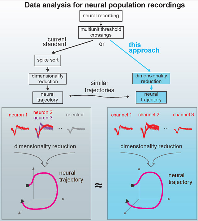
In a common type of extracellular electrophysiology experiment, a multi-electrode array provides researchers access to a sparse sample of a few hundred neurons, selected somewhat randomly from the much larger number of neurons in a particular brain region. For most typical experiments, spike sorting is performed prior to subsequent analysis steps, such as performing dimensionality reduction and then regressing the resulting ‘neural state’ against some behavioral measurement. The process of spike sorting changes the dimensionality of the dataset from the number of recording channels to the total number of isolatable neurons observed in the experiment (Figure 1A). Depending on how many neurons are sorted, this can expand or reduce the overall dimensionality of the data. Here, we propose to bypass this sorting step prior to population-level analyses. Dimensionality reduction methods, such as PCA, GPFA, dPCA, or TCA, typically use linear combinations of individual sorted neurons to capture important aspects of the population response in a reduced representation of the data, hereafter referred to as a “manifold” (Yu et al., 2009; Churchland et al., 2012; Brendel et al., 2011; Kobak et al., 2016; Gallego et al., 2017; Pandarinath et al., 2018; Williams et al., 2018) (Figure 1B). By starting with multi-unit threshold crossings, the spikes from multiple neurons observed on each channel are linearly summed prior to performing a second linear operation via dimensionality reduction. The resulting manifold representing the neural population activity may closely resemble that found with sorted neurons, shown schematically in Figure 1C.

Figure 1: Estimation of neural dynamics using multi-unit threshold crossings.

A) Data acquisition and pre-processing steps. The experimentally measured dimensionality of neural activity in the motor system suggests that a small number of latent factors (typically 8-12 in the primate motor system for simple behavioral tasks) captures the majority of task-relevant neural variability. In most experiments, neural recordings are sparsely sampled from up to a few hundred or thousand neurons in systems containing many millions of neurons. B,C) Standard practice is to sort spikes from individual neurons using action potential waveforms and perform dimensionality reduction on the smoothed firing rates of the isolated units. Here, we propose that for certain specific classes of analyses, it’s theoretically and pragmatically sensible to bypass the sorting step and perform dimensionality reduction or population-level analyses on voltage threshold crossings directly.

This approach is motivated not only by the success of BMI threshold crossing decoders, but more fundamentally by the theory of random projections from high dimensional statistics (Indyk & Motwani, 1998; Dasgupta & Gupta, 2003; Ganguli & Sompolinsky, 2012; Advani et al., 2013; Lahiri et al., 2016). Recent work has shown that if one wishes to recover the geometry of a low dimensional manifold that is embedded in a high dimensional space, one can still accurately recover this geometry without measuring all of the coordinates of the high dimensional space. Instead, it is sufficient to measure a small number of noisy, random linear combinations (i.e., projections) of these coordinates (Ganguli & Sompolinsky, 2012). In the neuroscience context, (1) the low dimensional manifold is a surface containing the set of low dimensional neural population trajectories (so-called underlying ’latent factors’ (Shenoy et al., 2013; Gallego et al., 2017)); (2) the coordinates in high dimensional space are the firing rates or spike counts of all individual neurons relevant to the behavior; and (3) the noisy projections of these coordinates are the spiking activity measured across all electrodes. The spiking activity on a single electrode is comprised of a linear combination of isolatable spikes from a small number of neurons near that electrode, as well as smaller spikes that cannot be attributed to individual neurons, sometimes referred to as “hash”. Here, we use the term “multiunit activity” to refer to the combination of isolatable single units plus hash. This application of random projection theory to neural measurements suggests that spike sorting may not be necessary to accurately recover neural population dynamics for many experimentally-relevant conditions. Importantly, we will show that if the neural activity manifold is relatively low dimensional and smooth across time, and the tuning properties of neurons on the same electrode are not strongly anti-correlated, then it should be possible to recover the manifold geometry without spike-sorting, given enough multi-unit recording channels.

We tested whether combining multiple units prior to applying dimensionality reduction algorithms significantly distorts the reduced-dimensionality estimates of neural state using a combination of empirical data, simulations, and theory. We used Neuropixels probes to record from populations of several hundred neurons simultaneously in dorsal premotor (PMd) and primary motor (M1) cortex, and found that neural trajectories are only minimally distorted when starting from multi-unit threshold crossings or simulated multi-unit channels. In addition, we replicated analyses from three previously published studies of nonhuman primate motor cortical control of arm movements, now using multiunit threshold crossings (i.e., the linear combination of a small number of neurons as well as multiunit ‘hash’). We compared the resulting unsorted neural population state dynamics and hypothesis testing outcomes with those of the original studies (which did spike sort). We found that all of the new analyses using multi-unit threshold crossings closely recapitulated both qualitative and quantitative features found in the original studies and yielded the same scientific conclusions. We further show that the similarity of neural population dynamics extracted from sorted versus unsorted data is consistent with the theory of random projections, and we derive quantitative scaling laws for how this similarity depends both on the complexity of the population dynamics and the number of recording channels.

We suggest that these findings may: (1) unlock existing data for new analyses without time-consuming manual sorting or error-prone automatic sorting, (2) inform the design and use of new wireless, low power electrode arrays for laboratory investigations and clinical use (in particular, chronically-implanted multielectrode arrays and bandwidth and power limited wireless telemetry systems), and (3) enable scientific measurements using electrode arrays that do not afford high quality spike sorting, which enables long-term electrophysiological studies.

Results

Building intuition through a toy example

It may seem surprising that it is possible to accurately estimate neural population state without spike sorting, especially when signals from multiple neurons with potentially dissimilar tuning properties are combined onto the same recording channel. To build intuition for how and when this approach can work, we first present a toy example. We also discuss a more complete theory based on random projections in a later section. In this toy example, we simulated a population of neurons with Gaussian tuning to a single task parameter. This tuning could reflect, for example, the average firing rate of neurons in primary visual cortex, as a function of the angular orientation of a grating, or the firing rate of neurons in primary motor cortex as a function of reach direction. Figure 2A illustrates an instance of this simulation, in which the tuning curves of multiple neurons on each channel are highly correlated, resulting in multiunit tuning curves which generally resemble those of the single units (Figure 2B). Applying PCA to the population activity of multiunit channels results in a low-dimensional manifold which closely resembles the one calculated using single neurons (Figure 2C). Here we define the distortion, ϵ, as the worst case fractional error in distances between all pairs of points on all trajectories, measured in a state-space defined by electrodes, relative to the state-space defined by single neurons (see Methods, and also Lahiri and colleagues for a detailed discussion (Lahiri et al., 2016)). Thus Figure 2A-C reflects the intuitive situation in which combining information from different neurons on the same recording channel results in little loss of tuning, because all neurons on the same channel have similar tuning curves.

Figure 2: Simulation of neural manifold estimation without spike sorting for a simple 1D system.

200 channels of simulated neural activity using simulated neurons with randomly generated tuning to a 1D parameter (e.g.: reach angle). Neurons tuning curves on each channel exhibit correlation ρ (see methods) and neurons on different channels are uncorrelated. (A) Tuning curves for three example channels with six units per channel with strongly correlated tuning (ρ = 0.8). (B) Multiunit tuning curves for each channel shown above. (C) (top) PCA-projected firing rate manifold, projected onto the first two principal components, estimated using simulated single units depicted in (A). (bottom) PCA-projected firing rate manifolds, estimated using multiunit channels depicted in (B). (D) As in (A,B,C), but with uncorrelated tuning curves (ρ = 0). (E) As in (A,B,C), but with anticorrelated tuning curves (ρ = −0.2). (F) Distortion of manifolds resulting from combining units for different single unit correlation strengths (see equation (2) in methods). Vertical dotted lines indicate the worst case anticorrelation. (G) Root mean square (RMS) error in estimating 1D parameter (direction) for different tuning correlation strengths. Dashed horizontal lines show the RMS error using spikes from separate units. Solid lines show the RMS error using multiunit channels. (H) Examples firing rate manifolds for spike sorted units (first column) and multiunit channels (second column) for various levels of distortion.

However, it is not necessary for all neurons on the same channel to have similar tuning curves. Even if neurons on each channel are uncorrelated (ρ = 0), it is still possible to accurately recover the geometry of the neural manifold using multiunit channels (Figure 2D). It is only when neural tuning curves are explicitly anti-correlated (e.g.: ρ ≤ −0.2) that the manifold becomes more distorted (Figure 2E). Figure 2F illustrates the manifold distortion as a function of the number of neurons on each electrode and the correlation in tuning curves between those neurons. For the region where ρ is between 0 and 1, distortion scales only modestly with the number of neurons recorded per channel and is largely insensitive to the correlation among units. Large distortions are only observed when neurons on each electrode are pathologically anti-correlated, such that their respective contributions cancel out, resulting in each multiunit channel exhibiting minimal tuning.

As a complementary test of whether not spike sorting corrupts our ability to estimate behavior from neural activity, we attempted to decode the 1D parameter (e.g., reach angle) from the population of synthetic multi-unit channels (Figure 2G) and real neural data (Supplementary Figure S1G). This revealed that decoding accuracy was high across a wide range of synthetic data tuning correlations and for the real data. Figure 2H provides examples of manifolds with varying levels of distortion to provide intuition as to how this metric affects inferred latent dynamics.

Thus overall, this toy example continuously interpolates between two intuitive and extreme scenarios of highly correlated or uncorrelated neurons on each channel. If the multiple neurons recorded on the same channel have strongly correlated (anti-correlated) tuning curves, then combining them leads to similar (destroyed) channel tuning, and dimensionality reduction yields accurate (distorted) neural manifolds. Interestingly, this toy example reveals that uncorrelated tuning curves, corresponding to randomly recorded neurons on the same electrode, does lead to reduced tuning on each channel, but nevertheless manifold geometry can be accurately recovered given enough channels. Thus, only scenarios in which neurons on the same channel have explicitly anti-correlated tuning can impair neural population state estimation if the other stated assumptions are true. Importantly, we do not observe this explicit anti-correlation within local groups of neurons in experimental data (Supplementary Figure S2B-D). Finally, we obtained similar results when simulating an oscillatory neural system (Supplementary Figure S1A-F).

Estimating neural population dynamics in a motor reaching task

We next asked whether using multi-unit activity instead of isolated single units leads to distortions in the neural activity manifolds by analyzing experimental data from the motor cortex of rhesus monkeys recorded while they performed an instructed delay reaching task. Neural trajectories during reaches to eight radially spaced targets using neurons recorded using two Utah arrays implanted in PMd and M1 reveal substantial similarity between neural trajectories obtained using sorted units and multi-unit threshold crossings (Figure 3A). We repeated this comparison using neural data recording using Neuropixels probes in PMd, which allow for high confidence in the spike sorting, since virtually all recorded neurons are visible to multiple recording sites along the probe (Jun et al., 2017b) (Figure 3B). Units were spike sorted using Kilosort and Phy to provide the automated and manual cluster curation steps respectively, to ensure single unit isolations and neuron stability over the course of a recording session (Supplementary Figure S3).

Figure 3: Neural trajectories from primate motor cortex during reaches are similar with and without spike sorting.

(A) Neural trajectories for delayed reaches to one of eight radial targets using manually sorted neurons (left) or unsorted multi-unit spikes (right) obtained by thresholding the voltage time-series at −4.5 × the root mean square (RMS) of the voltage time series. Trajectories display little distortion in the low-dimensional projections using PCA. Data collected using chronically implanted Utah microelectrode arrays. (B) Same as (A), for data collected using acute Neuropixels probes. Simulated multi-unit activity was generated by randomly combining the activity of between 1-4 sorted neurons per channel (without replacement).

We observed that manifold distortion was relatively low when using multi-unit threshold crossings in place of isolated single neurons for Utah array and Neuropixels data. We tested this both via explicitly recombining sorted neurons into multi-unit channels (Figure 3B, middle) and directly using multi-unit threshold crossings for neuropixel data (Figure 3B, right), using the manifold distortion metric employed previously and described in detail in Methods. We note that the Neuropixel’s dense electrode spacing causes many neurons to appear on multiple channels, increasing the correlation between channels and reducing the number of independent random projections along the probe (Supplementary Figures S2 and S3). This results in larger distortion than the Utah array or simulated multi-unit datasets, as predicted by the previous simulations and theory. Even in this more correlated oversampling regime, the distortion is modest. Nonetheless, these results argue in favor of sparser sampling of more neurons, rather than more views of the same neurons, if the goal is to better estimate the neural population state. We will revisit this argument in the Discussion. We also note that this distortion metric is defined as the worst-case distortion between pairs of vectors on two manifolds, and the average distortion is considerably lower in most cases.

While these qualitative findings are suggestive, a quantitative study is required to assess how avoiding spike sorting would affect the conclusions of neuroscientific studies that examine population-level phenomena. We re-analyzed data collected in three recently published studies by Ames and colleages; Churchland, Cunningham, and colleagues; and Kaufman and colleagues (Ames et al., 2014; Churchland et al., 2012; Kaufman et al., 2014). All three studies relate the spiking activity of populations of neurons in macaque motor and dorsal premotor cortex to arm reaching behavior. Each study used acute single-unit recordings as well as population recordings using Utah multielectrode arrays to establish the findings presented, and the results were not sensitive to the recording method used. For each replication, we substitute multi-unit threshold crossings prior to replicating the analyses used in the original studies. As described below and in Methods, using a sufficiently stringent voltage threshold (typically at least −3.5 times the root mean square (RMS) value of the voltage on each channel) effectively rejects electrical artifacts and thermal noise. Thus, these multi-unit threshold crossings predominantly correspond to action potential emission from one or multiple neurons in the vicinity of the electrode. See Supplementary Figure S4 for a comparison of spike waveforms from sorted single units and multi-unit threshold crossings. As anticipated, the tuning for recording channels tends to broaden (Supplementary Figure S4D) and the mean firing rates increase (Supplementary Figure S4E) as the threshold becomes more permissive and includes spikes from more neurons. Here, we ask whether these anticipated observations at the level of individual channels result in large distortions in the geometry of the population activity structure, and whether this impacts the studies’ conclusions drawn from population-level analyses.

Study 1: Neural dynamics of reaching following incorrect or absent motor preparation

Ames and colleagues asked whether the preparatory neural population state achieved by motor cortex prior to the initiation of movement is obligatory for generating an accurate reach, either when no time is given to prepare the reach (no delay period) or when the target location switches at the time of the go cue (Ames et al., 2014). The key result of the study, found using manually spike-sorted data, was that in both cases the neural population state can bypass the preparatory state when no time is provided to prepare the movement. Visualizations of neural trajectories using the top two principal components (Figure 4A) reveal qualitatively similar features when using multi-unit threshold crossings instead of sorted neurons. Statistical tests of the key neural distance metric used in the original study show that the results are closely recapitulated when using unsorted data instead of isolated single neurons (Figure 4 B, p < 0.05, (Ames et al., 2014)). This provides empirical evidence that using multi-unit threshold crossings does not substantially distort the low-dimensional geometry of neural population dynamics or the scientific conclusions drawn from resulting estimates of the neural population state.

Figure 4: Replication of “Neural population dynamics during reaching (Ames et al., 2014)”.

(A) Neural trajectories calculated using PCA on trial-averaged neural activity for reaches with and without delay period using hand sorted units, a more conservative threshold set at −4.5 × RMS, a more permissive threshold set at −3.5 × RMS, using only threshold crossings that were discarded after sorting, and when sorted units were randomly combined to simulate multi-unit channels. (B) The key results from (Ames et al., 2014): distance in full-dimensional neural space between trial-averaged neural trajectories of reaches when the monkey was or was not presented with a delay period. Note that the vertical axis is scaled between columns, illustrating that although ensemble firing rates are higher with more permissive thresholds, the key qualitative and quantitative features of the population neural response are conserved. (C) Example unit 1: PSTHs for center-out reaches to eight radially spaced targets. In this example, firing rates scale higher with a more permissive threshold, but the overall shape of the PSTHs are similar regardless of sorting or thresholding. (D) Example unit 2: Features of the PSTHs for this unit do change as a more permissive threshold is used. Despite this variation, the estimated neural state from the population response, as shown in A is largely invariant to the choice of threshold.

We repeated these analyses with two simulated perturbations to the dataset to further test the sensitivity of population analyses to combining the contributions of individual neurons. First, we analyzed only the multi-unit threshold crossing events that were previously discarded through spike sorting. The computed neural trajectories, distance plots, and peri-stimulus time histograms (PSTHs) for these discarded spikes suggest that there is similar information content in these low-amplitude multi-unit ‘hash’ spikes as there are in the larger-amplitude, sortable individual neurons (Figure 4, fourth column). Second, we repeated these analyses after randomly recombining individual neurons to simulate multi-unit thresholded channels (minus the contribution of unsortable hash). The results for this manipulation also closely matched those found with sorted single neurons (Figure 4, fifth column). Note that the PSTHs for this case are not anticipated to resemble those of any particular single units, but are not shown to demonstrate that recombination of units does not substantially abolish neural tuning to the behavior (in this case, reach target).

Several observations are apparent from these analyses. First, for some electrode channels, the shape of the PSTHs across conditions is closely recapitulated regardless of the threshold level or inclusion of hash (Figure 4C). For these channels, the spatial and temporal properties of the constituent parts of the multi-unit threshold crossings (i.e., individual neurons and hash) are similar enough that combining these components results in a simple vertical scaling of the PSTHs that largely preserves their shapes. For other electrode channels, however, the inclusion of additional units via re-thresholding with a more permissive threshold does change the spatial and temporal tuning by adding neurons with different tuning properties (Figure 4D). Interestingly, however, when we consider all electrode channels together and reduce the dimensionality of the data using PCA, we find the resulting low-dimensional projections (i.e., the neural population state estimates) are not sensitive to these individual channel-level changes. For both the randomly recombined units and the discarded spikes, the resulting neural population analyses replicate the original findings derived from single neuron firing rates, including hypothesis tests evaluated with statistical criteria (e.g., p-values), and the resulting neural trajectories.

Study 2: Neural population dynamics during reaching

We tested this analysis method on a second study, conducted by Churchland, Cunningham, and colleagues, who described how neural population activity in macaque motor cortex exhibits strong rotational dynamics during reaching (Churchland et al., 2012) This result was also replicated later in humans as well (Pandarinath et al., 2015). The population rotational dynamics were revealed using jPCA, a dimensionality reduction algorithm that identifies 2D planes exhibiting rotational dynamics within the higher-dimensional neural state space. This study argues that motor cortex uses a set of oscillatory basis functions to construct the complex time-varying signals required to control muscles during a reach. Further statistical support for this observation has been provided by (Elsayed & Cunningham, 2017), demonstrating that the rotational dynamics are not an immediate consequence of smooth firing rates and applying dimensionality reduction algorithms to high-dimensional data.

The rotational dynamics described in (Churchland et al., 2012) arise from fast and limited-duration oscillatory patterns present in the firing rates of individual neurons. This temporal precision poses a specific test for whether multi-unit threshold crossings would reveal the same low-dimensional neural structure. Since each of the constituent units in the unsorted activity recorded on a single channel are not constrained to have similar relationships with behavioral parameters or time, a potential concern is that linearly combining them would distort the observed population dynamics by “washing out” the individual units’ temporally-precise tuning features. Thus, for this particular study, we might expect that combining oscillatory units with different periodicity or phases could decrease or eliminate rotatory dynamics at the level of the population.

We did not find this to be the case; rather, we found that using multi-unit threshold crossing data closely recapitulated Churchland, Cunningham and colleagues’ original findings. Applying jPCA to the original spike sorted data yields a jPC plane (2D) which captures 23% of the variance in the neural data. Applying the same analysis to threshold crossing data yielded planes which capture 23%, 23%, and 21% of the variance in neural data when using voltage thresholds of −3.5, −4.0, and −4.5 × RMS, respectively. The key rotatory structure in the neural data reported by Churchland and colleagues was also preserved and clearly present when using multi-unit threshold crossing data (Figure 5, S6). In addition, a key quantitative metric used in the original study, the ratio $R_{M_{\mathit{skew}}}^2∕R_M^2$, is quite similar between thresholded and neural data (Supplementary Figure S5).

Figure 5: Replication of “Neural population dynamics during reaching” (Churchland, Cunningham et al., 2012.

Neural trajectories from 108 conditions including straight and curved reaches using (A) Hand sorted units. (B-D) Unsorted multi-unit activity using a voltage threshold of −4.5, −4.0 and −3.5 × RMS. The total amount of variance captured in the top rotational plane and the qualitative features of neural population state space trajectories are similar across sorted units and all three threshold crossing levels.

While the precise location of individual neural trajectories may appear slightly different between sorted and thresholded data sets, the dominant rotatory structure apparent across conditions and time, as well as the quantitative hypothesis tests regarding this structure, are quite similar across these datasets. We also note that differences in trajectory positions may result from either manifold distortion or from viewing the manifold from a slightly different 2D projection. The precise location of neural trajectories in these plots is sensitive to the weighting coefficients for the 2D jPCA plane fits to the data, but we have not adjusted the jPCA weights or modified the viewing angle to maximize the similarity of the projections.

Study 3: Cortical activity in the null space: permitting preparation without movement

The third study we replicated sought to understand how there can be large changes in PMd and M1 firing rates during a preparatory instructed delay period, without causing the circuit’s downstream muscle targets to move (Kaufman et al., 2014). The mechanism the authors proposed is that the brain makes use of specific “output-null” dimensions in the neural state space (i.e., weighted combinations of firing rates of neurons that cancel out from the perspective of a downstream readout) to enable computation within a given circuit without influencing output targets. Other “output-potent” neural dimensions do not cancel out, resulting in signals which do cause muscle activity. Kaufman and colleagues showed that neural population activity patterns before movement occupy the putative output-null subspace, consistent with this hypothesis. This activity could be related to computation preparing the arm for movement (Shenoy et al., 2013), and/or cognitive processes such as a working memory of the behavioral goal (Rossi-Pool et al., 2016a). Importantly, the output-null and output-potent dimensions were not separate sets of neurons (i.e. separate pools of delay-active neurons and movement-only neurons) (Kaufman et al., 2014). Instead, these output-null and output-potent neural dimensions consisted of different weightings of the same neurons which were identified by contrasting the dominant modes within the low-dimensional population activity (found using PCA) between preparation and movement. Recently these subspaces have been shown to be orthogonal for a delayed reach task with recordings in PMd in rhesus macaques (Elsayed et al., 2016).

Kaufman and colleagues’ findings presents another distinct challenge for the threshold crossing approach: one might expect that combining multiple neurons could mix together output-potent and output-null dimensions. On the other hand, these dimensions are defined as weighted sums of the activity of all recorded neurons, and these neurons’ activities are themselves a mixture of output-potent and output-null signal components. Thus, it might not be surprising that measuring the firing rates of several neurons together would provide similar ability to identify the underlying output-null and output-potent dimensions from the higher-dimensional space formed by all recording channels. We re-analyzed the data presented by Kaufman and colleagues, which originally employed spike-sorting, and found that with 192 threshold crossing channels (96 electrodes each in PMd and M1), we observed the same distinction between output-potent and output-null neural dimensions as in the original study (Figure 6). Kaufman and colleagues quantified this effect using the ratio of variance of neural activity in output-null to output-potent dimensions during the preparatory epoch. They found this ratio was 5.6 (p = 0.021) using sorted units; here we found it to be 3.84 (p = 0.048) using −3.5 × RMS threshold crossings (Figure 6, dataset N20100812).

Figure 6: Replication of “Cortical activity in the null space: permitting preparation without movement” (Kaufman et al., 2014).

Comparison of output-null and output-potent neural activity during preparing and then executing movements using the original sorted and newly re-analyzed thresholded data. (A) Neural activity in one output-null and output-potent dimension for one data set (NA), as in Figure 4A,B in (Kaufman et al., 2014). Activity is trial-averaged, and each trace presents the neural activity for one condition. The horizontal bars indicate the epoch in which the ratio of output-null and output-potent activities reported in panels C and D was calculated (left) and the epoch from which the dimensions were identified (right). (B) Same as (A), computed using activity thresholded at −3.5 × RMS. (C) Tuning depth at each time point in output null and output potent dimensions, as in Figure 4C in (Kaufman et al., 2014). (D) Same ac (C), computed using activity thresholded at −3.5 × RMS.

The key feature to compare between the sorted and unsorted results in Figure 6 is the increase in the magnitude of neural activity in the output-null dimensions (Figure 6 A,B, top panels) following the input of target information, compared with very little such increase in output-potent dimensions (Figure 6 A,B, bottom panels). However, it is also evident that there are differences between the sorted and unsorted projections. This is because each of the plots in (Figure 6 A,B) represent projections along a 1D axis from a 3D space; as such, the shape of the plots is sensitive to the precise orientation of this axis, and we don’t expect that projections along this axis throughout the duration of the trial will look identical. While it would be possible to rotate bases to make these plots more visually similar, we’ve chosen to leave the non-rotated output as it recapitulates the key results from (Kaufman et al., 2014) while revealing that using unsorted spikes does superficially change the appearance of neural projections in this analysis. In addition, we observed a larger transient component in both the output-null and output-potent response following target appearance, as shown in Figure 6C,D. We speculate that this is because threshold crossings, which reflect the spikes from more overall neurons than examining sorted units, better detect a broad increase in firing rates when task-relevant sensory information arrives in motor cortex (Stavisky et al., 2017). Despite these secondary differences, the multi-unit threshold crossing analysis of these data replicates the key finding that motor cortical firing patterns are largely restricted to output-null dimensions during movement preparation.

Kaufman and colleagues’ study assessed whether preparatory activity is confined to a subspace orthogonal to that spanned by the putative output-potent movement-generating activity. This analysis uses PCA to find a 6D space, then partitions that space into two 3D subspaces, an output-potent and an output-null subspace. All neural activity, regardless of task-relevance, must exist in either of these two orthogonal subspaces; this addition of task-irrelevant ‘noise’ makes this analysis intrinsically hungry for statistical power. The p-values calculated using the original study’s most conservative metric (which includes all neural data following target presentation, including both the initially transient and steady state firing) were 0.269 and 0.554 for thresholds of −4.0 × RMS and −4.5 × RMS, respectively (compared to p=.021 using sorted neurons). The effect sizes are 2.006 and 1.926, respectively. However, the p-values calculated at steady state after target appearance were 0.042 (−4.0 × RMS) and 0.119 (−4.5) RMS, and the variance tuning ratio plots reveal similar structure. While these results are close, they do not quite reach a p-value of 0.05 significance level. We speculate that the statistical power would grow significantly with additional channels of threshold crossing data as was used for the other array dataset in (Kaufman et al., 2014) (which used threshold crossings in addition to spike sorted units). An independent validation of measuring the output-null hypothesis using threshold crossings (rather than sorted spikes) comes from our recent study which used BMI experiments to definitively show that the output-null mechanism isolates visuomotor feedback from prematurely affecting motor output (Stavisky et al., 2017).

To summarize our results involving the re-analysis of various scientific hypothesis, we selected three recent studies based on the potential challenges and insights they could offer for this investigation of using multi-unit threshold crossings instead of sorted single unit activity. For all three previously published studies considered here, the key scientific advances have been recapitulated using threshold crossings instead of individual neurons. While this outcome need not be the case for all studies, the fact that it worked for these three different studies, which span a variety of datasets, questions, and analysis techniques, suggests that it will generalize to many other population-level analyses of neural activity. This could enable many new scientific analyses, and we anticipate its relevance and importance to continue to grow as the number of recorded channels in experiments increases.

A random projection theory of recovering neural population dynamics using multi-unit threshold crossings

We observe that the low-dimensional neural population dynamics reported here using threshold crossings are very similar to those reported in previous studies that relied on single neurons isolated using spike-sorting methods. Given that combining action potentials from several neurons on each electrode channel discards some information, this result may seem surprising. Why does discarding information have such a small effect on the estimated dynamics? Before addressing this question, we first note that in practice, accepting unsortable threshold crossings also adds new information from spikes that could not be previously sorted. In this section, however, we restrict our considerations to the information-destroying operation of combining neurons. The relevant thought experiment is thus: even if we could sort all of those spikes (which in practice one cannot), would lumping them together actually distort the underlying neural trajectories by an unacceptable amount?

Here we use the theory of random projections to provide a quantitative explanation. Central to this explanation is the concept of a manifold, or a smooth, low dimensional surface containing the data. This explanation reveals that when a manifold embedded in a high dimensional space is randomly projected to a lower dimensional space, then the underlying geometry of the manifold will incur little distortion under the following conditions: (1) the manifold itself is simple (i.e., smooth, with limited volume and curvature), and (2) the number of projections is sufficiently large with respect to the dimensionality of the manifold. While true theoretically, the key practical question is, does this theory allow for accurate recovery of neural population dynamics under experimentally and physiologically relevant conditions?

To apply random projection theory to our data, we must first define the high-dimensional space and the low-dimensional manifold. In this neuroscientific application, the high dimensional space has one axis per neuron, with the coordinate on that axis corresponding to the firing rate of that neuron. Thus, the space’s full dimensionality is equal to the total number of neurons in the relevant brain area, which is much larger than the total number of neurons from which we are able to record. However, in many brain areas, particularly within the motor system, most neurons’ trial-averaged neural activity patterns vary smoothly across both time and behavioral-task conditions. Thus, as one traces out time and conditions, the resultant set of covarying neural activity patterns constitutes the embedded manifold in random projection theory (Gao & Ganguli, 2015) (i.e., blue curve in top-left of Figure 7A). Empirically, we find that the dimensionality of neural activity is far lower than the number of recorded neurons (Yu et al., 2009; Gallego et al., 2017; Rossi-Pool et al., 2016b). This is likely due in part to the structure of connections within the network, but may also be in part due to the fact that the experimental conditions do not fully span the set of possible behaviors. The manifold also has limited curvature, precisely because neural activity patterns vary smoothly across time and conditions. Thus, this neural manifold satisfies the condition of simplicity posited in random projection theory.

Figure 7: Random projection theory suggests spike sorting is often not necessary for population analyses.

(A) Schematic depiction of a projection of a trajectory through high-D firing rate space defined by single units, projected onto a subspace defined by the number of recording channels. A small amount of information is lost by combining units on each channel. Adding the contribution of multi-unit hash may introduced additional distortion to the estimated neural trajectories, though in practice this appears to be small. (B) Pearson correlation coefficient between single units on the same recording channel (blue) and different channels (green) for dataset N20101105. (C) Hash has a larger Pearson correlation coefficient (p < 0.05) with single units on the same channel (blue) than from other channels (green). Same dataset as (B). (D) PCA trajectories sampled from simulated random Gaussian manifolds were measured from (simulated) single neuron activities. Manifold mean and covariance were matched to those of neural activity from dataset N20101105 spike sorted data. (E) the same as (D) for threshold crossings data. (F) The maximum distortion of random one-dimensional manifolds under random projections of N = 125 neurons. The length of the manifolds, T (sec), and the number of manifolds, C, are varied with fixed correlation length, τ = 14.1. The 95th percentile of the distortions under 100 random projections is plotted (mean ± standard deviation for 50 repetitions). This collapses into a simple linear relationship when viewed as a function of ln (CT / τ), plotted for data (G) and for simulated random Gaussian manifolds (H).

Finally, the mapping from single neuron firing rates to threshold crossing activity constitutes a random projection itself: each electrode’s activity is a weighted linear combination of a small number of isolated neurons plus any additional hash that passes the threshold. Thus, the low dimensional space in random projection theory has dimensionality equal to the number of electrodes. The projection from neurons to electrodes is considered random because we assume the tuning curves of individual neurons across time and task parameters are uncorrelated, corresponding to the ρ = 0 scenario in Figure 2D. Within this low-dimensional space of electrodes (which itself is a subspace of the high dimensional space of neurons), neural activity traces out a simple manifold (Figure 7A) due to the even lower latent dimensionality of the activity.

This scenario raises the critical question: how much is the geometry of the manifold distorted when combining single-neuron firing rates within each electrode? To help answer this question, we generated random manifolds of neural activity using simulated single units and multi-unit firing rates, and estimated the dynamics of these random neural manifolds. In generating these synthetic data, we incorporated the average empirical correlation structure between single neurons (Figure 7B) and between single units and multi-unit threshold crossings on a given channel (Figure 7C) in a real monkey reaching dataset. Neural population state-space trajectories obtained from simulated single neurons (Figure 7D) closely match those obtained from simulated threshold crossings (Figure 7E). These results are consistent with and reinforce the previous sections’ comparisons of single unit-derived and threshold crossings-derived neural dynamics in real neural data.

Random projection theory enables us to go beyond this qualitative view and derive a quantitative theory of how the geometric distortion between threshold crossings and single-neuron neural population state-space trajectories depend on their underlying complexity and on the number of measurement channels (Donoho, 2006; Baraniuk & Wakin, 2009; Ganguli & Sompolinsky, 2012; Advani et al., 2013). Manifold distortion will depend on the volume and curvature of the trajectories. In the simple case where neural population dynamics consists of C different neural trajectories (corresponding to different behavioral conditions) each of trial duration T, the volume can be taken to be proportional to CT. In turn, the curvature is related to the inverse of the temporal auto-correlation length τ of the neural trajectories (Clarkson, 2008; Baraniuk & Wakin, 2009; Verma, 2011; Gao & Ganguli, 2015; Lahiri et al., 2016). Intuitively, τ (see Methods) measures how long one must wait before a neural trajectory curves appreciably, so that small (large) τ indicates high (low) curvature.

We can parametrically vary the complexity of neural population dynamics by analyzing subsets of neural trajectories of different durations T and subsets of conditions of different sizes C. In doing so for real data, we find that the distortion grows with both T and C (Figure 7F). However, random projection theory predicts a striking and specific scaling relation between the squared distortion ϵ² and the parameters T, C, and number of channels M. In particular it predicts that ϵ² scales linearly with $\frac{1}{M}\ln \left(\frac{CT}{\tau }\right)$ . Thus, distortion is predicted to be directly proportional to the logarithm of the product of manifold volume and curvature (i.e. $\frac{CT}{\tau }$), and inversely proportional to the number of recording channels M. This predicted scaling relation is seen both in real neural data (Figure 7G) and in simulations where the data was generated so as to match the overall average statistics of the recorded data (Figure 7H).

We note, however, that the distortion relationships found in the multiple datasets (and the simulated data generated based on their statistics) form different lines in (Figure 7G,F). One reason for the different lines is that these analyses deal not with deterministic random projections, but rather noisy random projections, in which the presence of hash introduces both signal and additional noise, or activity which is uncorrelated to the isolatable single neurons on a channel. A natural measure of signal to noise is the ratio of the variance of single unit activity, to the variance of that part of the hash that is not correlated with the single units. By fitting a generative model to the neural data, we can estimate this SNR (see Methods). For data collected from the two Utah arrays, We found the SNRs to be 1.9 for dataset N20101105 in (Ames et al., 2014) and 1.3 for dataset N20100812 in (Kaufman et al., 2014). Thus, as expected, both the recorded and simulated data incur higher distortion at fixed complexity $\frac{CT}{\tau }$ if the SNR is lower. Moreover, in the neuropixels dataset V20180818, the SNR is 1.6, but this recording array also picks up more neurons on each recording electrode, which increases the slope of the distortion line. However, in all cases, the distortion scales linearly with $\frac{1}{M}\ln \left(\frac{CT}{\tau }\right)$ (Figure 7GH), albeit with slightly different slopes and y-intercepts.

Thus this scaling relationship provides quantitative theoretical guidance for when we can expect to accurately recover neural population dynamics without spike sorting. Intuitively, analyzing threshold crossings makes sense when (1) neural trajectories are not too long (small T, e.g.: less than a few seconds), (2) not too curved (large τ), (3) not too many in number (small C), (4) the additional multiunit hash has small variance relative to that of single-units on the same electrode (non-negligible SNR), and (5) we have enough electrodes (large M). Under these conditions, neural dynamics can be accurately inferred using multi-unit threshold crossings. These conditions are satisfied in the datasets considered here, and are likely to be satisfied in many more. Notably, the dense sampling provided by a single Neuropixels probe provides fewer independent projections of neural activity than the number of recording channels, since most neurons are visible to multiple channels. Future studies of recordings from other brain regions, in other species, and across a range of whether the above properties hold true or not will be needed to further establish the generality of these experimental, analytical and theoretical findings.

Discussion

We investigated whether multi-unit threshold crossings can be used instead of isolated single neurons specifically to address questions involving neural population dynamics. We believe that this question is necessary and timely, as neuroengineers are currently engaged in a massive scale-up in the number of electrodes used to make measurements. At the same time, systems neuroscientists are increasingly building quantitative models to better understand how neural population dynamics give rise to behaviorally-relevant computations (Remington et al., 2018a, b; Wang et al., 2018; Vyas et al., 2018; Chaisangmongkon et al., 2017). Thus, the field is facing the question of the type of neural data (e.g., single neurons, multi-units, local field potentials) that will be important to record when thousands to millions of electrodes are available. Some of these questions are already starting to be confronted in the related but distinct endeavor of large-scale neural imaging using genetically-encoded calcium indicators (Sofroniew et al., 2016).

We report here both a theoretical justification and an empirical validation which together argue that many of the same scientific conclusions can be made about population-level motor cortical activity without spike sorting. We believe that these findings are broadly useful for several reasons. First, the process of spike sorting is both time consuming and inexact, with significant variability between experts (Wood & Black, 2008). For a typical experiment composed of many hours of neural recordings, an expert human sorter may spend several hours to make hundreds or thousands of small and uncertain decisions to manually sort spikes on a single 100-channel electrode array (e.g., “Utah array” (Maynard et al., 1997)). New high-channel-count recording technologies like Neuropixels are becoming available that will enable recording from thousands to millions of channels simultaneously. A data set composed of 1,000 channels could take over 100 hours to hand sort, with no ground truth available to validate results. Automated spike sorters may partially alleviate this burden, but even today’s state-of-the-art ‘automated’ sorters still require significant manual curation (e.g.: (Pachitariu et al., 2016; Chung et al., 2017; Chaure et al., 2018)). As reported here, if the goals of the scientific effort require describing population-level neural activity, then this effort (and its associated opportunity cost) is unlikely to impact the resulting insights about the population state and its dynamics.

Second, in real-world experimental conditions, chronically implanted multi-electrode arrays in animal models or in humans often feature many channels with neural activity that cannot be isolated into single neurons (e.g., (Pandarinath et al., 2015)) by either manual or automated sorting. Ignoring these channels throws out potentially meaningful task-related information, possibly weakening statistical power and subsequent scientific conclusions. Insisting on spike sorting in these situations would fail to capitalize on valuable experimental and clinical opportunities. Including such electrodes will enable analyses of larger datasets from more overall neurons (potentially across more brain areas) by making use of electrodes with fewer isolatable waveforms due to device age or random variability. At the same time, however, we recognize that not spike sorting is not a panacea when recording quality is limited. There will remain many important scientific questions that rely on single neuron isolation, which should motivate parallel work to improve sensor longevity and recording quality optimized for enabling spike sorting.

Third, these results support the design of novel classes of sensors for both scientific experimentation and BMI clinical trials, by allowing for sparser sampling and reducing the sampling rate and communication bandwidth required for implantable medical devices. We describe this in more detail below.

Finally, this study may help increase scientific reproducibility and reduce the number of animals or clinical trial participants required to achieve the same scientific goals. Regarding reproducibility of findings, removing the often subjective step of spike sorting, which is typically only vaguely described in publications’ methods, ought to increase the ability of multiple labs to replicate results from the same data set or to replicate findings as part of subsequent studies. By quantitatively and theoretically grounding the approach of using threshold crossings, large numbers of unused existing data sets can now be brought to bear on new hypotheses. Data sets collected using older electrode technologies, or where recording conditions prevent detection of well isolated cells, are likely appropriate for answering new questions without spike sorting. Re-use of previously collected data or collecting new data in existing subjects can therefore reduce the number of new subjects required. However, we stress that this method is not appropriate for scientific questions regarding individual neurons, such as questions regarding stimulus selectivity, precise spike timing between neurons, single cell tuning properties, cell type identification based on electrophysiological or other markers, and others. For these studies, we must either rely on closely clustered electrodes and automated sorting methods or restrict the number of analyzed neurons to what is feasible to hand sort.

We also stress that we are not advocating for loosening expectations with respect to data quality or scientific rigor. For example, experimenters must take care to ensure that recorded signals containing multiunit threshold crossings are stable over time, particularly for acute recordings where probe drift of 10’s of microns can cause neural signals to appear to change over time. It is also important to ensure that recordings are free of electrical artifacts or other sources of non-neural noise. No single prescription will ensure data quality, but it remains the responsibility of an experimentalist to ensure that their data sources capture the measurements of interest.

Lastly, it is important to note that this approach is comparing the geometry of low dimensional neural activity between multiunit threshold crossings and isolated single units recorded using a given recording method. If the distribution of recording electrodes only samples from a specific subset of neurons, then distortions or biases may be introduced in the estimates of neural population dynamics regardless of whether isolated single units or multiunit channels are used for the analysis. By combining multiple units via the use of threshold crossings in place of isolated units, we take a random projection of the units that were already visible to electrodes. The argument that we put forward is that this process does not create large distortions in the observable manifold of neural activity, as compared the single neuron analyses that could have been made with the same original recordings.

Applicability of this paradigm

The Johnson-Lindenstrauss lemma from high-dimensional statistics shows that manifold estimation error increases as the complexity of the underlying manifold increases (Johnson & Lindenstrauss, 1984). The studies replicated here have all focused on neural recordings from PMd and M1, where roughly 10-15 dimensions capture 90% of the variability of trial-averaged neural population activity when monkeys perform a simple 2D reaching task (e.g., (Yu et al., 2009)). Recording from one or two Utah arrays (i.e., 96 or 192 electrodes) provides sufficiently redundant sampling of these lowdimensional manifolds. In this regime, we robustly find that we can replicate scientific hypotheses using voltage threshold crossings in place of well isolated single units. However, we anticipate that during substantially more complex behavioral tasks, the underlying neural state will be higher dimensional and thus will potentially require sampling from more electrodes to accurately identify the underlying manifold.

One might expect that it is important for constituent projections of the low-dimensional activity manifold (in this case multi-unit recording channels) to preserve the tuning properties of the individual neurons. This might initially seem to indicate that not spike sorting would be problematic in areas like cortex, where a number of recent studies have revealed that tuning properties of closely spaced neurons can be quite different (e.g.: (Machens et al., 2010; Kaufman et al., 2014; Rossi-Pool et al., 2016a)). We observed a similar lack of clustering of tuning properties of nearby neurons in macaque PMd in the high-density Neuropixel recordings presented here (Supplementary Figure S2, which allowed for a more precise characterization of the functional properties of nearby neurons than is possible using lower-density Utah arrays or laminar probes. Importantly, however, the theory of random projections suggests that our ability to accurately estimate the geometry of the low-dimensional activity manifold does not depend on the orientation of the manifold with respect to the full dimensional embedding space. Nor is it sensitive to the mixture of tuning properties of individual neurons, as long as the neurons’ tuning is not negatively correlated. Thus, we can combine the activity of neurons with different tuning properties without significantly distorting our estimates of the neural activity manifold, provided that the activity manifold is smooth and we have enough independent projections of the data. This theoretical prediction is supported by the empirical comparisons of numerous datasets’ sorted vs. unsorted neural trajectories and resulting scientific conclusions presented here.

The use of multi-unit threshold crossings is not appropriate for establishing whether neurons exhibit selective tuning to one or more stimuli or task parameters. In such an investigation, combining multiple units could erroneously lead one to conclude that units share selectivity to multiple stimuli. If, however, a scientific investigation seeks to understand how information about task parameters is encoded at the level of the population, then using threshold crossings may be appropriate, as the estimates of the low-dimensional neural state should be similar regardless of whether the input sources were single units or multi-unit channels. Intriguingly, numerous previous studies have observed mixed selectivity of individual neurons to multiple task parameters in animals (Rigotti et al., 2013; Mante et al., 2013; Rossi-Pool et al., 2016a; Hardcastle et al., 2017; Rossi-Pool et al., 2017; Murray et al., 2017) and in humans (Kamiński et al., 2017). Supervised dimensionality reduction methods, such as Demixed Principal Components Analysis (dPCA), can then be used to find linear dimensions which capture variance attributable to different task parameters (Machens et al., 2010; Kobak et al., 2016). This approach is compatible with the use of multi-unit threshold crossings since, as we have shown, the geometry of the low dimensional activity manifold is preserved. We further predict that this result should not be highly sensitive to the specific choice of dimensionality reduction methods, and we anticipate that dimensionality reduction of threshold crossings will ‘work’ (in the sense of revealing underlying neural state) for a wide range of algorithms, such as LDA, dPCA (Kobak et al., 2016), LFADS (Pandarinath et al., 2018), in addition to the PCA and jPCA methods used here.

The observation of relatively low-dimensional neural population dynamics is well established in the motor system (e.g.: (Yu et al., 2009; Churchland et al., 2012; Gallego et al., 2017)), but may not be true for all brain regions. In other brain areas, particularly input-driven sensory areas, the dimensionality of neural activity may be significantly higher or scale rapidly with the complexity of a sensory stimulus, resulting in more complex activity manifolds with higher curvature (Cowley et al., 2016). Under these other conditions, it remains to be determined how many independent random projections (multi-unit recording channels) would be required to accurately recover the underlying structure of neural activity. Similarly, if a particular neural signal of interest is small with respect to the total neural variance, it may (but is not guaranteed to) incur larger relative distortions than high-variance signals. In principle, accurate manifold geometry measurement should be possible with sufficient independent multi-unit recording channels, but this remains to be empirically tested in other brain areas and other species. Code is provided to calculate manifold distortion is provided in supplementary materials.

Implications for neural sensor design

These findings provide a scientific rationale for developing both acute and chronic multielectrode arrays which feature many thousands to millions of electrode channels at the expense of discarding information necessary to sort individual neurons. Virtually all existing acute and chronic electrophysiology systems are designed with the ability to record high sample rate data from each channel (e.g., digitizing 30,000 samples per second), which facilitates spike sorting. Relaxing these constraints reduces the storage and processing requirements for acute experiments and enables low power, high-channel count devices for clinical applications, where size, power, and communication bandwidth requirements constrain the number of channels. For acute experiments, saving only the spike times for multi-unit threshold crossings reduces the total data volume between 4 and 5 orders of magnitude relative to full broadband data. This is especially relevant for future clinical applications, where wireless neural data communication is necessary. Radios consume higher power as data volume increases with increasing sampling rate and bit depth. The present work argues that for many applications, simple spike threshold detection is sufficient in lieu of precise and high sample rate data to enable subsequent spike sorting. This suggests developing chronically-implantable electrode arrays with integrated electronics for spike detection and wireless-data transmission of only threshold crossings, which would significantly reduce power consumption and communication bandwidth. This will enable dramatically higher total channel count for a given implant size and power budget (e.g.: (Chestek et al., 2009; O’Driscoll et al., 2011)).

For any fixed number of electrodes to be distributed throughout some volume of tissue (e.g., across the surface of the cortex, in depth through cortex, as well as in deeper structures), there exists a trade-off between the goals of spike sorting, which benefits from closer electrode spacing, and recording from a larger number of neurons distributed through a larger volume. For example, the newly-developed Neuropixels probes enable a user to select a subset of 384 active channels from a total of 966 along a single-shank silicon probe (Jun et al., 2017b). By selecting a sparse subset of the active channels, a user can elect to trade off additional tissue coverage for spike sorting quality at the outset of an experiment. Obtaining additional coverage should enable less biased sampling by enabling recording from a larger number of neurons distributed more broadly throughout cortical lamina or multiple brain regions.

In this study we’ve examined threshold crossings using a relatively stringent criterion (≤ −3.5 × RMS), which identifies putative action potentials from one or a few cells near the electrode. A related but distinct question that warrants future work is whether performing similar analyses on the lower-amplitude spiking information examined by using features like high gamma (Pandarinath et al., 2017), continuous ‘multiunit activity’ (Stark & Abeles, 2007), or threshold crossings as low-voltage as −1.0 × RMS (Perel et al., 2015) would also reveal similar underlying neural state dynamics. These studies found that these more inclusive neural features often contained more information about motor behavior than well-isolated neurons, which we believe is consistent with our argument that an additional benefit of not spike sorting is that it can take advantage of useful neural information that is not sufficiently isolatable to identify as a putative single neuron.

This study reinforces the idea that selecting an appropriate sensor depends on both the scientific goals of an experiment and the structure of activity in the recorded brain region. In brain areas whose neural population activity is governed by low-dimensional dynamics, a sensor that prioritizes quantity of independent neural channels (more random projections) over quality of unit isolation (facilitating spike sorting) may be appropriate. In other words, sparser sampling from more brain volume will likely be advantageous for such studies.

Conclusions

The experimental neuroscience paradigm proposed here, using threshold crossings, applies to neural population-level analyses. It is not applicable in cases where one wishes to make statements about the properties (e.g. stimulus selectivity) of individual neurons. We nonetheless anticipate that this approach is broadly applicable to systems neurophysiology and is relevant not only to the analysis of experimental data, but also to the design and use of new chronic electrode arrays and acute multi-site recording probes. Analyzing threshold crossing spikes rather than sorted single unit activity will facilitate efficient and informative neural population analyses in ever-growing neurophysiology datasets. New sensors designed to maximize the number of threshold crossing channels (even at the cost of single unit isolation) may enable next-generation brain-machine interfaces with considerably greater capabilities, performance and robustness. The present work demonstrates that this method is theoretically justified, empirically supported, and simple to use.

Methods

Contact for reagents and resource sharing

Further information and requests for resources and reagents should be directed to and will be fulfilled by the Lead Contact, Eric Trautmann (etraut@stanford.edu).

Experimental model and subject details

All surgical and animal care procedures were performed in accordance with National Institutes of Health guidelines and were approved by the Stanford University Institutional Animal Care and Use Committee. Detailed information on the individual subjects used in the three reanalyzed experiments are provided in the original reports. (Ames et al., 2014; Churchland et al., 2012; Kaufman et al., 2014). All three experiments, as well as the newly collected Neuropixels probe datasets, employed head-fixed rhesus macaque monkeys making reaching movements in a 2D vertical workspace to touch targets presented on a touchscreen. The Neuropixels experiments were performed using an adult male monkey (Mucacct Mulatta) V (12 kg, 8 years old) who had a recording chamber placed over left hemisphere PMd/M1 and performed reaches with the right arm.

Method details

Task design

Details of the experimental task designs and detailed procedures for the three previous studies whose data was re-analyzed here using threshold crossings, including these studies’ behavioral analyses, neural recordings, and neural analyses, have been detailed previously in (Ames et al., 2014; Churchland et al., 2012; Kaufman et al., 2014). In each of these studies, rhesus macaque monkeys were trained to make delayed reaching movements to targets presented on a touch screen. For the Neuropixels datasets, monkeys were trained to move an onscreen cursor using a 3D haptic manipulandum confined to move within a 2D vertical work space. The haptic manipulandum did not apply any forces to the monkeys arm and was only used for passive cursor control. These experiments employed the same delayed reach task used in the three Utah array dataset experiments above. Delay periods were distributed uniformly with 90% of trials between 200 - 650 ms and 10% 0 ms delay.

Targets of 2 cm diameter were presented at 12mm from the center hold target at one of 24 radially-spaced targets. Juice reward was delivered automatically after a fixed target hold period. Failure resulted in no reward and an error tone. The period starting from the instructed delay and ending with the target acquisition (or failure) constituted a trial.

Neuropixels probe data acquisition and spike sorting

Neuropixel datasets were acquired using Neuropixels Phase 3A probes supplied by IMEC and Janelia. Recordings were performed using a custom 3D printed probe holder mounted to a microelectrode drive (NAN instruments). Prior to insertion, the dura was prepared by creating a small perforation using a 22-gauge needle with internal stylet to make a small perforation (approx. 700μ) in the dura prior to probe insertion, then visually aligning the probe to the perforation during insertion. A stainless steel tube was placed 1.5-3 mm off to the side of the insertion location and held with another electrode drive tower in order to provide gentle downwards pressure to stabilize cortical tissue with respect to the probe and to serve as an electrical reference for all channels on the probe. No guide tube was used during insertion due to the short shank (10 mm) of the Neuropixels probe.

Data were acquired from the 384 channels closest to the probe tip covering 3.84 mm and fully spanning cortical lamina in premotor and primary motor cortex. Data were acquired with SpikeGLX software at 30 KHz with an amplifier gain of 500 for each channel and high-pass filtered with a cutoff frequency of 300 Hz. Spike sorting was performed using Kilosort to automatically cluster units from raw data (Pachitariu et al., 2016). The resulting spike clusters were manually curated to split and merge clusters using Phy Template-gui software. Neurons were sorted using the sorting guidelines provided by Kwik Team (https://phy-contrib.readthedocs.io/en/latest/template-gui/#a-typical-approach-to-manual-clustering). Individual neurons were inspected to insure that the waveform template across multiple channels was consistent with a single neuron, that there was a low incidence of refractory period violations, and that the template amplitude was relatively constant throughout the full duration of the recording period. Clusters which violated any of these properties, suggesting either the inclusion of spikes from multiple neurons or a lack of temporal stability in firing properties (e.g., if the unit was only visible for a portion of the experimental session) were excluded from all analyses presented here. In practice, approximately 350 neurons were recorded during each experimental session using a single Neuropixels probe. For a given session, roughly 150-250 of these units were isolatable as single unit and stable throughout the duration of the session. Example unit isolations using the Phy Template-gui are shown in Supplementary Figure S3. Clusters were then analyzed in MATLAB using the sortingQuality package to identify clusters with ≥ 3% ISI violations (ISI ≤ 2 ms) (https://github.com/cortex-lab/sortingQuality).

Utah array recording and data processing

For all three experiment replication datasets, monkeys performed a delayed point to point reaching task to targets presented on a touch screen while neural data was recorded from two Utah arrays (Blackrock Microsystems, USA) placed in PMd and M1 of the contralateral hemisphere. Raw neural recordings (voltage measurements taken at 30,000 Hz) were first high-pass filtered above 250 Hz (4-pole, “spikes medium” setting) by the Blackrock neural recording system. Then, voltage snippets around measurements that crossed a threshold at −3.5 × root mean square voltage level for a given channel were saved. Spike sorting for the original studies was performed by hand, based on grouping spikes by similarity of waveform (i.e., assigning them to putative single neurons). For the present study’s re-analyses, rethresholded datasets were constructed by calculating new voltage threshold levels for each channel, and retaining the subset of original waveforms that also crossed the more conservative thresholds at −4.0 and −4.5 × RMS. Threshold crossings, regardless of waveform shape, were treated as spike events and processed further into temporally-smoothed, trial-averaged PSTHs prior to subsequent analyses such as PCA (Ames et al., 2014; Kaufman et al., 2014) or jPCA (Churchland et al., 2012).

The result obtained by Kaufman and colleagues is particularly hungry for statistical power, as it simply involves a binary partition of a 6D space, and looks for differences in activity at different time points in the two subspaces. For this study, after re-thresholding data, noisy and/or weakly modulated units were removed using an SNR threshold. For this context, SNR as a unit’s modulation depth (i.e., maximum minus minimum trial-averaged firing rate) across all conditions and time, divided by the peak of that unit’s standard deviation across all conditions and time. Sweeping the SNR rejection threshold between 0 and 1.2 results in rejecting 0 to 8.8% of units, respectively (−3.5 RMS dataset). The calculated p-value varies between a maximum of 0.065 (no unit SNR filtering) and a minimum of 0.0475 across this range.

Neural data analysis

Analyses for each of the three replication studies using original spike sorted data and multi-unit thresholded data were performed using the same analytical methods described in each of original studies. Neuropixel data (both spike sorted and multi-unit thresholded data) were pre-processed by aligning spike trains to movement onset and smoothing with a 25 ms s.d. Gaussian kernel. Only successful trials with relatively straight reaches for trials with delay periods greater than 200 ms were included in the analysis. Data from 350 ms before movement onset until 500 ms were trial averaged prior to performing PCA and calculating manifold distortion.

Simulated multiunit channels were created by combining the spiking activity from 1-3 randomly selected channels (without replacement). Hash-only channels were calculated by extracting the spikes discarded during spike sorting and performing analyses on these spikes only.

Population activity simulation

In order to evaluate how sensitive neural population analyses are to not spike sorting, we generated synthetic neural population activity based on simulated neurons with known tuning properties for a one-dimensional parameter θ, where 0 ≤θ ≤2π. We used a functional form for the tuning curves given by:

$$r_i(\theta )=r_0\text{exp}\left(a_i\cos (\theta -{\varphi }_i)\right).$$

The parameter r₀ represents the baseline firing rate and a_i scales the range of the response. The peak response for a given neuron is centered around ϕ_i.

The tuning curves are computed from two dimensional vectors, (x, y), drawn from zero mean unit variance Gaussian distributions:

$$x_i={\tanh }^{-1}(a_i)\cos {\varphi }_i,\langle x_i{x}_j\rangle =\langle y_i{y}_j\rangle =(1-\rho ){\delta }_{ij}+\rho ,$$ (1)

$$y_i={\tanh }^{-1}(a_i)\sin {\varphi }_i,\langle x_i{y}_j\rangle =0.$$

where i and j index different neurons contributing to the same channel. The hyperbolic tangent ensures that the amplitude is bounded, a_i ≤ 1. The correlation strength must lie in the interval $-\frac{M}{N-M}\le \rho \le 1$. We averaged the RMS error and distortion over 100 random samples of tuning curves for each value of ρ.

For maximum likelihood estimation in the asymptotic limit of large data sets, the estimator variance is equal to the inverse of the Fisher information. The Fisher information from separate units is

$$F=\sum _i\frac{1}{r_i}{\left(\frac{\mathrm{d}{r}_i}{\mathrm{d}\theta }\right)}^2.$$

The Fisher information from combined units is

$$F=\frac{1}{{\sum }_i{r}_i}{\left(\sum _i\frac{\mathrm{d}{r}_i}{\mathrm{d}\theta }\right)}^2.$$

The total Fisher information is the sum of the above over channels. The RMS error is then $1∕\sqrt{F_{\text{total}}}$.

Definition of the Distortion of Manifolds under a Projection

Let r be a high-dimensional vector of single neuron firing rates at an instant of time. Let e be the corresponding thresholded, temporally smoothed electrode activities at the same time. They are related via a noisy projection e = Ar + h where each element of the matrix A is the probability that a spike from that neuron produces a voltage deflection that crosses threshold in that electrode, and the noise vector h indicates the additional contribution of noise that passes the threshold. The geometric distortion of a single electrode pattern e, relative to a firing rate pattern r is defined as

$$ϵ=\mid \frac{\lambda \Vert \mathbf{e}\Vert -\Vert \mathbf{r}\Vert }{\Vert \mathbf{r}\Vert }\mid ,$$ (2)

where λ is a scale factor, used to remove the effect of multiplication of all vectors by a single scalar. Here · denotes the length of a vector, and so the distortion is the fractional change in length up to a scale λ.

The distortion of a set of manifolds is computed by finding the maximum distortion of the vectors between all pairs of points on any of the manifolds, including those between different manifolds. The scale factor λ is chosen to minimize the maximum distortion of the manifold set, thereby correcting for trivial overall changes in scale induced by the projection. Thus the distortion of a set of manifolds is the worst case fractional error in pairwise distances, up to an overall scale.

A generative model for neural manifolds and their projections

To quantitatively test how well the framework of random projections of smooth manifolds matches neural data, we developed a generative model of neural state space dynamics in single neuron firing rate space, its projection to electrodes, and the addition of noise. We modeled the neural population dynamics themselves as a random smooth manifold.

We generated 50 different such manifolds and their noisy projections by sampling T × C × (N + M) numbers (firing rates) from a multivariate Gaussian distribution, with mean and covariance chosen to have the same statistics as in the data, where T is the number of time points in a neural trajectory, C is the number of conditions, N is the number of single units and M is the number of recording channels (192 in this case). The multivariate Gaussian distribution we used corresponds to the following generative model for the peristimulus time histograms (PSTHs) of single units, r_n, multi-unit hash, h_μ, and channels, e_μ:

$$\begin{gathered} e_{\mu }(t,c)=\sum _n{\mathit{A}}_{\mu n}{r}_n(t,c)+h_{\mu }(t,c), \\ {r}_n(t,c)=R(t,c)+{\beta }_r\left(z_n(t,c)+k_{r}z(t,c)\right), \\ {h}_{\mu }(t,c)=H(t,c)+{\beta }_h\left({ϵ}_{\mu }(t,c)+k_hϵ(t,c)\right)+\frac{1}{N}\sum _n\left(M{k}_s{\mathit{A}}_{\mu n}+k_d\right)r_n(t,c), \end{gathered}$$

where A is a random projection matrix, described in more detail below, and z_n(t, c), z(t, c), ϵ_μ (t, c), and ϵ(t, c) are independent Gaussian random processes whose autocovariance across time and conditions were set equal to corresponding quantity computed from data, normalized to have unit total variance. The functions R(t, c), H (t, c), and the constants β_r, k_r, β_h, k_h, k_s, k_d, were fit to the data by setting the means, standard deviations and correlation coefficients of r_n and h_μ in the model equal to the mean of the corresponding quantity in the data. The constant k_r accounts for correlations between single units, k_h for correlations between hashes, k_d for correlations between hash and single units, and k_s for the stronger correlations between hash and single units on the same channel.

In this generative model it is possible to separate the simulated unsorted activity, e_μ, into noise (the terms proportional to β_h) and signal (everything else). This allows us to calculate a signal-to-noise ratio for each dataset after fitting the model parameters, defined as the ratio of the variances of signal and noise.

For each manifold set, 100 random projections, A, were sampled as described in the next section. For each random projection and random manifold set, the distortion of the manifold set was computed as described above. The 95th percentile of the distortions under the 100 projections was recorded. The mean and standard deviation of these distortion percentiles was taken over the 50 manifold sets.

Distortion of PSTHs

The PSTHs of the spike sorted data were taken to be the set of unprojected manifolds and the thresholded data was taken to be the set of projected manifolds. The distortion of the manifolds was then computed as described above.

Correlations of PSTHs

The covariance matrix across time and conditions was computed from spike sorted data by treating each neuron as a sample. The normalized covariance matrix was computed by dividing the covariance matrix by the total variance across time and conditions. To compute the correlation time, this covariance was then averaged for pairs of times with the same separation. This covariance function was then fit to a sum of two Gaussians centered at zero. The correlation time τ was then computed by matching the value and second derivative at zero to that of a single Gaussian. The correlation coefficients and standard deviations of single units and hash were computed from spike sorted data by treating each time point and condition as a sample.

Key resources table

REAGENT or RESOURCE	Source	Identifier
Experimental Models: Organisms/Strains
Rhesus macaque (Mucacca mulatta)	Wisconsin, Davis, and Yerkes Primate Centers	N/A
Software and Algorithms
MATLAB	Mathworks	https://www.mathworks.com/products/matlab.html
Simulink	Mathworks	https://www.mathworks.com/products/simulink-real-time.html
Kilosort	Cortex Lab GitHub	https://github.com/cortex-lab/KiloSort
Phy Template-gui	Kwikteam GitHub	https://github.com/kwikteam/phy
SpikeGLX	Bill Karsch GitHub	http://billkarsh.github.io/SpikeGLX/
Data Acquisition
Neuropixels probes	Janelia / IMEC	Phase 3A
Utah Microelectrode Arrays	Blackrock Microsystems	http://blackrockmicro.com/electrode-types/utah-array/
Cerebus system	Blackrock Microsystems	http://blackrockmicro.com/neuroscience-research-products/neural-data-acquisition-systems/cerebus-daq-system/
NAN Microdrive	NAN Instruments	http://naninstruments.com/index.php?todo=product-link&id=23

Highlights:

• For population analyses, spike sorting often has minor impact on estimates of neural state.

• Multiunit activity creates a random projection of low-dimensional neural state.

• Results from three prior studies in macaque PMd/M1 were replicated without spike sorting.

• Neuropixels probes used to provide high quality unit isolation in primate motor cortex.

References

- Advani M, Lahiri S, & Ganguli S (2013). Statistical mechanics of complex neural systems and high dimensional data. J. Stat. Mech, 2013, P03014. [Google Scholar]
- Ajiboye AB, Willett FR, Young DR, Memberg WD, Murphy BA, Miller JP, Walter BL, Sweet JA, Hoyen HA, Keith MW, Peckham PH, Simeral JD, Donoghue JP, Hochberg LR, & Kirsch RF (2017). Restoration of reaching and grasping movements through brain-controlled muscle stimulation in a person with tetraplegia: a proof-of-concept demonstration. Lancet, 389, 1821–1830. [DOI] [PMC free article] [PubMed] [Google Scholar]
- Ames KC, Ryu SI, & Shenoy KV (2014). Neural dynamics of reaching following incorrect or absent motor preparation. Neuron, 81, 438–451. [DOI] [PMC free article] [PubMed] [Google Scholar]
- Baraniuk RG & Wakin MB (2009). Random projections of smooth manifolds. Foundations of Computational Mathematics, 9, 51–77. [Google Scholar]
- Bargmann C, Newsome W, Anderson A, Brown E, Deisseroth K, Donoghue J, MacLeish P, Marder E, Normann R, Sanes J, & Others (2014). BRAIN 2025: a scientific vision. Brain Research Through Advancing Innovative Neurotechnologies (BRAIN) Working Group Report to the Advisory Committee to the Director, NIH. Available online at: http://www.nih.gov/science/brain/2025/(US National Institutes of Health, 2014). [Google Scholar]
- Barnett AH, Magland JF, & Greengard LF (2016). Validation of neural spike sorting algorithms without ground-truth information. Journal of Neuroscience Methods, 264, 65–77. [DOI] [PubMed] [Google Scholar]
- Barrese JC, Rao N, Paroo K, Triebwasser C, Vargas-Irwin C, Franquemont L, & Donoghue JP (2013). Failure mode analysis of silicon-based intracortical microelectrode arrays in non-human primates. J. Neural Eng, 10, 066014. [DOI] [PMC free article] [PubMed] [Google Scholar]
- Bestel R, Daus AW, & Thielemann C (2012). A novel automated spike sorting algorithm with adaptable feature extraction. J. Neurosci. Methods, 211, 168–178. [DOI] [PubMed] [Google Scholar]
- Brendel W, Romo R, & Machens CK (2011). Demixed Principal Component Analysis. Advances in Neural Information Processing Systems, pp. 2654–2662. [Google Scholar]
- Briggman KL, Abarbanel HDI, & Kristan WB Jr (2005). Optical imaging of neuronal populations during decision-making. Science, 307, 896–901. [DOI] [PubMed] [Google Scholar]
- Chah E, Hok V, Della-Chiesa A, Miller JJH, O’Mara SM, & Reilly RB (2011). Automated spike sorting algorithm based on laplacian eigenmaps and k-means clustering. J. Neural Eng, 8, 016006. [DOI] [PubMed] [Google Scholar]
- Chaisangmongkon W, Swaminathan SK, Freedman DJ, & Wang X-J (2017). Computing by robust transience: how the fronto-parietal network performs sequential, category-based decisions. Neuron, 93, 1504–1517. [DOI] [PMC free article] [PubMed] [Google Scholar]
- Chaure FJ, Rey HG, & Quian Quiroga R (2018). A novel and fully automatic spike-sorting implementation with variable number of features. Journal of Neurophysiology, 120, 1859–1871. [DOI] [PMC free article] [PubMed] [Google Scholar]
- Chestek CA, Gilja V, Nuyujukian P, Foster JD, Fan JM, Kaufman MT, Churchland MM, Rivera-Alvidrez Z, Cunningham JP, Ryu SI, & Shenoy KV (2011). Long-term stability of neural prosthetic control signals from silicon cortical arrays in rhesus macaque motor cortex. J. Neural Eng, 8, 045005. [DOI] [PMC free article] [PubMed] [Google Scholar]
- Chestek CA, Gilja V, Nuyujukian P, Kier RJ, Solzbacher F, Ryu SI, Harrison RR, & Shenoy KV (2009). HermesC: low-power wireless neural recording system for freely moving primates. IEEE Trans. Neural Syst. Rehabil. Eng, 17, 330–338. [DOI] [PubMed] [Google Scholar]
- Christie BP, Tat DM, Irwin ZT, Gilja V, Nuyujukian P, Foster JD, Ryu SI, Shenoy KV, Thompson DE, & Chestek CA (2015). Comparison of spike sorting and thresholding of voltage waveforms for intracortical brain-machine interface performance. J. Neural Eng, 12, 016009. [DOI] [PMC free article] [PubMed] [Google Scholar]
- Chung JE, Magland JF, Barnett AH, Tolosa VM, Tooker AC, Lee KY, Shah KG, Felix SH, Frank LM, & Greengard LF (2017). A fully automated approach to spike sorting. Neuron, 95, 1381–1394.e6. [DOI] [PMC free article] [PubMed] [Google Scholar]
- Churchland MM, Cunningham JP, Kaufman MT, Foster JD, Nuyujukian P, Ryu SI, & Shenoy KV (2012). Neural population dynamics during reaching. Nature, 487, 51–56. [DOI] [PMC free article] [PubMed] [Google Scholar]
- Clarkson KL (2008). Tighter bounds for random projections of manifolds In Proceedings of the Twenty-fourth Annual Symposium on Computational Geometry, SCG ‘08, pp. 39–48. (New York, NY, USA: ACM; ). [Google Scholar]
- Collinger JL, Wodlinger B, Downey JE, Wang W, Tyler-Kabara EC, Weber DJ, McMorland AJC, Velliste M, Boninger ML, & Schwartz AB (2013). High-performance neuroprosthetic control by an individual with tetraplegia. Lancet, 381, 557–564. [DOI] [PMC free article] [PubMed] [Google Scholar]
- Cowley BR, Smith MA, Kohn A, & Yu BM (2016). Stimulus-Driven population activity patterns in macaque primary visual cortex. PLoS Comput. Biol, 12, e1005185. [DOI] [PMC free article] [PubMed] [Google Scholar]
- Dasgupta S & Gupta A (2003). An elementary proof of a theorem of johnson and lindenstrauss. Random Struct. Algorithms, 22, 60–65. [Google Scholar]
- Donoho DL (2006). Compressed sensing. IEEE Trans. Inf. Theory, 52, 1289–1306. [Google Scholar]
- Elsayed GF & Cunningham JP (2017). Structure in neural population recordings: an expected byproduct of simpler phenomena? Nature Neuroscience, 20, 1310–1318. [DOI] [PMC free article] [PubMed] [Google Scholar]
- Elsayed GF, Lara AH, Kaufman MT, Churchland MM, & Cunningham JP (2016). Reorganization between preparatory and movement population responses in motor cortex. Nat. Commun, 7, 13239. [DOI] [PMC free article] [PubMed] [Google Scholar]
- Fraser GW, Chase SM, Whitford A, & Schwartz AB (2009). Control of a brain-computer interface without spike sorting. J. Neural Eng, 6, 055004. [DOI] [PubMed] [Google Scholar]
- Gallego JA, Perich MG, Miller LE, & Solla SA (2017). Neural Manifolds for the Control of Movement. Neuron, 94, 978–984. [DOI] [PMC free article] [PubMed] [Google Scholar]
- Ganguli S & Sompolinsky H (2012). Compressed sensing, sparsity, and dimensionality in neuronal information processing and data analysis. Annu. Rev. Neurosci, 35, 485–508. [DOI] [PubMed] [Google Scholar]
- Gao P & Ganguli S (2015). On simplicity and complexity in the brave new world of large-scale neuroscience. Curr. Opin. Neurobiol, 32, 148–155. [DOI] [PubMed] [Google Scholar]
- Gilja V, Nuyujukian P, Chestek CA, Cunningham JP, Yu BM, Fan JM, churchland MM, Kaufman MT, kao JC, Ryu SI, & Shenoy KV (2012). A high-performance neural prosthesis enabled by control algorithm design. Nature Neuroscience, 15, 1752–1757. [DOI] [PMC free article] [PubMed] [Google Scholar]
- Gilja V, Pandarinath C, Blabe CH, Nuyujukian P, Simeral JD, Sarma AA, Sorice BL, Perge JA, Jarosiewicz B, Hochberg LR, Shenoy KV, & Henderson JM (2015). Clinical translation of a high-performance neural prosthesis. Nat Med, 21, 1142–1145. [DOI] [PMC free article] [PubMed] [Google Scholar]
- Hardcastle K, Ganguli S, & Giocomo LM (2017). Cell types for our sense of location: where we are and where we are going. Nature Neuroscience, 20, 1474–1482. [DOI] [PMC free article] [PubMed] [Google Scholar]
- Harris KD, Quiroga RQ, Freeman J, & Smith SL (2016). Improving data quality in neuronal population recordings. Nat. Neurosci, 19, 1165–1174. [DOI] [PMC free article] [PubMed] [Google Scholar]
- Harvey CD, Coen P, & Tank DW (2012). Choice-specific sequences in parietal cortex during a virtual-navigation decision task. Nature, 484, 62–68. [DOI] [PMC free article] [PubMed] [Google Scholar]
- Hochberg LR, Bacher D, Jarosiewicz B, Masse NY, Simeral JD, Vogel J, Haddadin S, Liu J, Cash SS, van der Smagt P, & Donoghue JP (2012). Reach and grasp by people with tetraplegia using a neurally controlled robotic arm. Nature, 485, 372–375. [DOI] [PMC free article] [PubMed] [Google Scholar]
- Indyk P & Motwani R (1998). Approximate nearest neighbors: towards removing the curse of dimensionality. Proceedings of the thirtieth annual ACM symposium on Theory of computing, pp. 604–613. [Google Scholar]
- Jarosiewicz B, Sarma AA, Bacher D, Masse NY, Simeral JD, Sorice B, Oakley EM, Blabe C, Pandarinath C, Gilja V, Cash SS, Eskandar EN, Friehs G, Henderson JM, Shenoy KV, Donoghue JP, & Hochberg LR (2015). Virtual typing by people with tetraplegia using a self-calibrating intracortical brain-computer interface. Sci Transl Med, 7, 313ra179–313ra179. [DOI] [PMC free article] [PubMed] [Google Scholar]
- Johnson WB & Lindenstrauss J (1984). Extensions of lipschitz mappings into a hilbert space. Contemp. Math, 26, 1. [Google Scholar]
- Jun JJ, Mitelut C, Lai C, Gratiy S, Anastassiou C, & Harris TD (2017a). Real-time spike sorting platform for high-density extracellular probes with ground-truth validation and drift correction. bioRxiv. [Google Scholar]
- Jun JJ, Steinmetz NA, Siegle JH, Denman DJ, Bauza M, Barbarits B, Lee AK, Anastassiou CA, Andrei A, Aydın Ç, Barbic M, Blanche TJ, Bonin V, Couto J, Dutta B, Gratiy SL, Gutnisky DA, Häusser M, Karsh B, Ledochowitsch P, Lopez CM, Mitelut C, Musa S, Okun M, Pachitariu M, Putzeys J, Rich PD, Rossant C, Sun W-L, Svoboda K, Carandini M, Harris KD, Koch C, O’Keefe J, & Harris TD (2017b). Fully integrated silicon probes for high-density recording of neural activity. Nature, 551, 232–236. [DOI] [PMC free article] [PubMed] [Google Scholar]
- Kamiński J, Sullivan S, Chung JM, Ross IB, Mamelak AN, & Rutishauser U (2017). Persistently active neurons in human medial frontal and medial temporal lobe support working memory. Nature Neuroscience, 20, 590–601. [DOI] [PMC free article] [PubMed] [Google Scholar]
- Kao JC, Nuyujukian P, Ryu SI, & Shenoy KV (2016). A high-performance neural prosthesis incorporating discrete state selection with hidden markov models. IEEE Trans. Biomed. Eng. [DOI] [PubMed] [Google Scholar]
- Kaufman MT, churchland MM, Ryu SI, & Shenoy KV (2014). Cortical activity in the null space: permitting preparation without movement. Nature Neuroscience, 17, 440–448. [DOI] [PMC free article] [PubMed] [Google Scholar]
- Kaufman MT, Churchland MM, Ryu SI, & Shenoy KV (2015). Vacillation, indecision and hesitation in moment-by-moment decoding of monkey motor cortex. eLife, 4:e04677. [DOI] [PMC free article] [PubMed] [Google Scholar]
- Kobak D, Brendel W, Constantinidis C, Feierstein CE, Kepecs A, Mainen ZF, Qi X-L, Romo R, Uchida N, & Machens CK (2016). Demixed principal component analysis of neural population data. eLife, 5:e10989. [DOI] [PMC free article] [PubMed] [Google Scholar]
- Koroshetz W, Gordon J, Adams A, Beckel-Mitchener A, Churchill J, Farber G, Freund M, Gnadt J, Hsu NS, Langhals N, Lisanby S, Liu G, Peng GCY, Ramos K, Steinmetz M, Talley E, & White S (2018). The State of the NIH BRAIN Initiative. Journal of Neuroscience, 38, 6427–6438. [DOI] [PMC free article] [PubMed] [Google Scholar]
- Lahiri S, Gao P, & Ganguli S (2016). Random projections of random manifolds. Arxiv. [Google Scholar]
- Leibig C, Wachtler T, & Zeck G (2016). Unsupervised neural spike sorting for high-density microelectrode arrays with convolutive independent component analysis. J. Neurosci. Methods, 271, 1–13. [DOI] [PubMed] [Google Scholar]
- Machens CK, Romo R, & Brody CD (2010). Functional, but not anatomical, separation of “what” and “when” in prefrontal cortex. J. Neurosci, 30, 350–360. [DOI] [PMC free article] [PubMed] [Google Scholar]
- Mante V, Sussillo D, Shenoy KV, & Newsome WT (2013). Context-dependent computation by recurrent dynamics in prefrontal cortex. Nature, 503, 78–84. [DOI] [PMC free article] [PubMed] [Google Scholar]
- Maynard EM, Nordhausen CT, & Normann RA (1997). The Utah intracortical electrode array: a recording structure for potential brain-computer interfaces. Electroencephalogr. Clin. Neurophysiol, 102, 228–239. [DOI] [PubMed] [Google Scholar]
- Morcos AS & Harvey CD (2016). History-dependent variability in population dynamics during evidence accumulation in cortex. Nat. Neurosci, 19, 1672–1681. [DOI] [PMC free article] [PubMed] [Google Scholar]
- Murray JD, Bernacchia A, Roy NA, Constantinidis C, Romo R, & Wang X-J (2017). Stable population coding for working memory coexists with heterogeneous neural dynamics in prefrontal cortex. Proceedings of the National Academy of Sciences of the United States of America, 114, 394–399. [DOI] [PMC free article] [PubMed] [Google Scholar]
- O’Driscoll S, Shenoy KV, & Meng TH (2011). Adaptive resolution ADC array for an implantable neural sensor. IEEE Trans. Biomed. Circuits Syst, 5, 120–130. [DOI] [PubMed] [Google Scholar]
- Pachitariu M, Steinmetz NA, Kadir SN, Carandini M, & Harris KD (2016). Fast and accurate spike sorting of high-channel count probes with KiloSort. Advances In Neural Information Processing Systems, pp. 4448–4456. [Google Scholar]
- Pandarinath C, Gilja V, Blabe CH, Nuyujukian P, Sarma AA, Sorice BL, Eskandar EN, Hochberg LR, Henderson JM, & Shenoy KV (2015). Neural population dynamics in human motor cortex during movements in people with ALS. eLife, 4, e07436. [DOI] [PMC free article] [PubMed] [Google Scholar]
- Pandarinath C, Nuyujukian P, Blabe CH, Sorice BL, Saab J, Willett FR, Hochberg LR, Shenoy KV, & Henderson JM (2017). High performance communication by people with paralysis using an intracortical brain-computer interface. eLife, 6:e18554. [DOI] [PMC free article] [PubMed] [Google Scholar]
- Pandarinath C, O’Shea DJ, Collins J, Jozefowicz R, Stavisky SD, kao JC, Trautmann EM, Kaufman MT, Ryu SI, Hochberg LR, Henderson JM, Shenoy KV, Abbott LF, & Sussillo D (2018). Inferring single-trial neural population dynamics using sequential auto-encoders. Nature methods, 15, 805–815. [DOI] [PMC free article] [PubMed] [Google Scholar]
- Perel S, Sadtler PT, Oby ER, Ryu SI, Tyler-Kabara EC, Batista AP, & Chase SM (2015). Single-unit activity, threshold crossings, and local field potentials in motor cortex differentially encode reach kinematics. J. Neurophysiol, 114, 1500–1512. [DOI] [PMC free article] [PubMed] [Google Scholar]
- Remington ED, Egger SW, Narain D, Wang J, & Jazayeri M (2018a). A dynamical systems perspective on flexible motor timing. Trends in cognitive sciences, 22, 938–952. [DOI] [PMC free article] [PubMed] [Google Scholar]
- Remington ED, Narain D, Hosseini EA, & Jazayeri M (2018b). Flexible sensorimotor computations through rapid reconfiguration of cortical dynamics. Neuron, 98, 1005–1019. [DOI] [PMC free article] [PubMed] [Google Scholar]
- Rigotti M, Barak O, Warden MR, Wang X-J, Daw ND, Miller EK, & Fusi S (2013). The importance of mixed selectivity in complex cognitive tasks. Nature, 497, 585–590. [DOI] [PMC free article] [PubMed] [Google Scholar]
- Rossant C, Kadir SN, Goodman DFM, Schulman J, Hunter MLD, Saleem AB, Grosmark A, Belluscio M, Denfield GH, Ecker AS, Tolias AS, Solomon S, Buzsaki G, Carandini M, & Harris KD (2016). Spike sorting for large, dense electrode arrays. Nat. Neurosci, 19,634–641. [DOI] [PMC free article] [PubMed] [Google Scholar]
- Rossi-Pool R, Salinas E, Zainos A, Alvarez M, Vergara J, Parga N, & Romo R (2016a). Emergence of an abstract categorical code enabling the discrimination of temporally structured tactile stimuli. Proceedings of the National Academy of Sciences, 113, E7966–E7975. [DOI] [PMC free article] [PubMed] [Google Scholar]
- Rossi-Pool R, Salinas E, Zainos A, Alvarez M, Vergara J, Parga N, & Romo R (2016b). Emergence of an abstract categorical code enabling the discrimination of temporally structured tactile stimuli. Proceedings of the National Academy of Sciences. [DOI] [PMC free article] [PubMed] [Google Scholar]
- Rossi-Pool R, Zainos A, Alvarez M, Zizumbo J, Vergara J, & Romo R (2017). Decoding a Decision Process in the Neuronal Population of Dorsal Premotor Cortex. Neuron, 96, 1432–1446.e7. [DOI] [PubMed] [Google Scholar]
- Sadtler PT, Quick KM, Golub MD, Chase SM, Ryu SI, Tyler-Kabara EC, Yu BM, & Batista AP (2014). Neural constraints on learning. Nature, 512, 423–426. [DOI] [PMC free article] [PubMed] [Google Scholar]
- Santhanam G, Sahani M, Ryu S, & Shenoy K (2004). An extensible infrastructure for fully automated spike sorting during online experiments. Conf. Proc. IEEE Eng. Med. Biol. Soc, 6, 4380–4384. [DOI] [PubMed] [Google Scholar]
- Shenoy KV, Sahani M, & Churchland MM (2013). Cortical control of arm movements: A dynamical systems perspective. Annual Review of Neuroscience, 36, 337–359. PMID: 23725001. [DOI] [PubMed] [Google Scholar]
- Sofroniew NJ, Flickinger D, King J, & Svoboda K (2016). A large field of view two-photon mesoscope with subcellular resolution for in vivo imaging. eLife, 5, e14472. [DOI] [PMC free article] [PubMed] [Google Scholar]
- Stark E & Abeles M (2007). Predicting Movement from Multiunit Activity. Journal of Neuroscience, 27, 8387–8394. [DOI] [PMC free article] [PubMed] [Google Scholar]
- Stavisky SD, kao JC, Ryu SI, & Shenoy KV (2017). Motor Cortical Visuomotor Feedback Activity Is Initially Isolated from Downstream Targets in Output-Null Neural State Space Dimensions. Neuron, 95, 195–208.e9. [DOI] [PMC free article] [PubMed] [Google Scholar]
- Stevenson IH & Kording KP (2011). How advances in neural recording affect data analysis. Nat. Neurosci, 14, 139–142. [DOI] [PMC free article] [PubMed] [Google Scholar]
- Todorova S, Sadtler P, Batista A, Chase S, & Ventura V (2014). To sort or not to sort: the impact of spike-sorting on neural decoding performance. J. Neural Eng, 11, 056005. [DOI] [PMC free article] [PubMed] [Google Scholar]
- Vargas-Irwin C & Donoghue JP (2007). Automated spike sorting using density grid contour clustering and subtractive waveform decomposition. J. Neurosci. Methods, 164, 1–18. [DOI] [PMC free article] [PubMed] [Google Scholar]
- Ventura V (2009). Automatic spike sorting using tuning information. Neural Comput, 21, 2466–2501. [DOI] [PMC free article] [PubMed] [Google Scholar]
- Verma N (2011). A note on random projections for preserving paths on a manifold. (Department of Computer Science and Engineering, University of California, San Diego: ). [Google Scholar]
- Vyas S, Even-Chen N, Stavisky SD, Ryu SI, Nuyujukian P, & Shenoy KV (2018). Neural population dynamics underlying motor learning transfer. Neuron, 97, 1177–1186. [DOI] [PMC free article] [PubMed] [Google Scholar]
- Wang J, Narain D, Hosseini EA, & Jazayeri M (2018). Flexible timing by temporal scaling of cortical responses. Nature Neuroscience. [DOI] [PMC free article] [PubMed] [Google Scholar]
- Williams AH, Kim TH, Wang F, Vyas S, Ryu SI, Shenoy KV, Schnitzer M, Kolda TG, & Ganguli S (2018). Unsupervised Discovery of Demixed, Low-Dimensional Neural Dynamics across Multiple Timescales through Tensor Component Analysis. Neuron, 98, 1099–1115.e8. [DOI] [PMC free article] [PubMed] [Google Scholar]
- Wood F & Black MJ (2008). A nonparametric bayesian alternative to spike sorting. J. Neurosci. Methods, 173, 1–12. [DOI] [PMC free article] [PubMed] [Google Scholar]
- Wood F, Black MJ, Vargas-Irwin C, Fellows M, & Donoghue JP (2004). On the variability of manual spike sorting. IEEE Trans. Biomed. Eng, 51, 912–918. [DOI] [PubMed] [Google Scholar]
- Wouters J, Kloosterman F, & Bertrand A (2018). Towards online spike sorting for high-density neural probes using discriminative template matching with suppression of interfering spikes. Journal of Neural Engineering, 15, 056005–16. [DOI] [PubMed] [Google Scholar]
- Yu BM, Cunningham JP, Santhanam G, Ryu SI, Shenoy KV, & Sahani M (2009). Gaussian-process factor analysis for low-dimensional single-trial analysis of neural population activity. J Neurophys, 102, 1881–1888. [DOI] [PMC free article] [PubMed] [Google Scholar]
Associated Data
This section collects any data citations, data availability statements, or supplementary materials included in this article.