Abstract
Background
Various methods for differential expression analysis have been widely used to identify features which best distinguish between different categories of samples. Multiple hypothesis testing may leave out explanatory features, each of which may be composed of individually insignificant variables. Multivariate hypothesis testing holds a non-mainstream position, considering the large computation overhead of large-scale matrix operation. Random forest provides a classification strategy for calculation of variable importance. However, it may be unsuitable for different distributions of samples.
Results
Based on the thought of using an ensemble classifier, we develop a feature selection tool for differential expression analysis on expression profiles (i.e., ECFS-DEA for short). Considering the differences in sample distribution, a graphical user interface is designed to allow the selection of different base classifiers. Inspired by random forest, a common measure which is applicable to any base classifier is proposed for calculation of variable importance. After an interactive selection of a feature on sorted individual variables, a projection heatmap is presented using k-means clustering. ROC curve is also provided, both of which can intuitively demonstrate the effectiveness of the selected feature.
Conclusions
Feature selection through ensemble classifiers helps to select important variables and thus is applicable for different sample distributions. Experiments on simulation and realistic data demonstrate the effectiveness of ECFS-DEA for differential expression analysis on expression profiles. The software is available at http://bio-nefu.com/resource/ecfs-dea.
Keywords: Feature selection, Classification, Accumulation, Expression profiles, Differential expression analysis
Background
Differential expression analysis (DEA) is widely adopted to identify a feature for best characterizing the expression difference between groups of individuals (e.g., healthy ones and those affected with a disease) [1]. Multiple hypothesis testing, which evaluates more than one hypothesis simultaneously, plays an important role in DEA. Corresponding tools such as SAM [2], limma [3], multtest [4], etc. have been produced for detecting differentially expressed variables. As a matter of fact, multiple hypothesis testing may leave out an explanatory signature. A selected feature expressed differently may not be composed of individually significant variables [5]. Although multivariate hypothesis testing may choose a proper feature, it still holds a non-mainstream position [6], considering the need for a large computation overhead of large-scale matrix operation.
Unlike statistical hypothesis testing, classification-based feature selection concentrates on better classification results of a certain subspace in many aspects such as sequence analysis [7, 8], site identification [9–12], protein classification [13, 14], protein identification [15, 16], protein fold recognition [17–19], protease substrate prediction [20, 21] and protein backbone torsion angle prediction [22]. Thus, predictive variables [23–25] are selected according to classification results of a certain classifier. Random forest [26, 27] is a case in point. It utilizes decision trees as the base classifier, which may be unsuitable for different distributions of samples. We have developed JCD-DEA [28], which is a feature selection tool combining hypothesis testing with classification strategy. However, JCD-DEA employs a bottom-up feature enumeration strategy, which is time consuming.
In this paper, we develop a top-down classification-based feature selection tool, i.e. ECFS-DEA, for differential expression analysis. In addition to random forest (RF), one of the other three classifiers, i.e., Fisher’s linear discriminant analysis (LDA), k-nearest-neighbor (kNN) and support vector machine (SVM), can be interactively selected to be the base classifier in accordance with different sample distributions. Under the development environment of Python 3.5, ECFS-DEA applicable to various execution environments such as a personal computer, a workstation or a large-scale cluster in Windows, Linux or Mac, can be used to identify the feature which best distinguishes between different categories of samples on expression profiles such as RNA-seq data, microarrays, etc.
Method
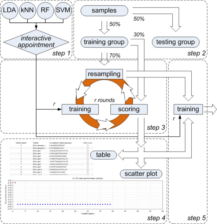
ECFS-DEA offers two main functions, i.e. feature selection and feature validation. Feature selection part contains five steps, as illustrated in Fig. 1. Firstly, the category of the base classifier is to be interactively appointed. RF, LDA, kNN and SVM are the alternative base classifier. The base classifier number r is also to be set. Meanwhile, the path of the input file, the data format and the execution environment are to be selected. Secondly, samples are randomly divided into training and testing groups in balance. Thirdly, a resampling procedure is constructed for the accumulation of variable importance. The resampling round is equivalent to the number of the base classifiers. In each round j, 70% of training samples are randomly selected in the entire feature space for training each classifier; while, the remaining 30% of training samples are the out-of-bag data for calculating the classification error rate Errj. As to each variable i, only one time permutation of its expression levels on the out-of-bag data is made, and the corresponding classification error rate is presented as . After r rounds of resampling, the importance of variable i is achieved as . Fourthly, a feature can be manually selected in a table with the individual variables sorted in descending order according to achieved variable importance or in a 2-D scatter plot with its horizontal and vertical coordinates corresponding to the variable indices and the accumulated importance, respectively. Fifthly, an ensemble classifier composed of r same base classifiers is to be trained using the expression levels of the training samples on the selected feature.
Fig. 1.
Schematic of feature selection part in ECFS-DEA
As to feature validation part, the testing samples are needed. Aiming at the expression levels of the testing set on the selected feature, a scatter plot in 1-D, 2-D or 3-D subspace can be illustrated. The corresponding ROC curve is also provided. Besides, a projection heatmap which displays discrete projection values (i.e., classification results) from the expression levels of the selected feature, is presented. Using the trained classifier, the classification results of the testing set on the selected feature are reordered based on k-means clustering. Accompanied with the expression levels and the labels, the reordered classification results are shown in the projection heatmap.
Implementation
ECFS-DEA is written mainly in Python 3.5, distributed under GNU GPLv3. Considering the existence of repeating steps in ECFS-DEA, we make a two-step implementation: a client part in Client.zip for executing GUI, and a server part in Server.zip which is designed to run on the cluster server that using Portable Batch System(PBS) as scheduling program. The client part also contains codes for analyzing expression profiles, if ECFS-DEA can only run on a personal computer or a workstation.
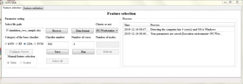
The parameter setting step of feature selection part is illustrated in Fig. 2. The file path, data format, execution environment, etc. are set. Besides, the category of the base classifier is interactively assigned. The number of the base classifier which is also the resampling round needs to be appointed. Sample splitting is performed after parameter setting. Once the accumulation of variable importance is fulfilled, the obtained scores can be listed in a table or a scatter plot form for manual selection, as illustrated in Figs. 3 and 4 respectively.
Fig. 2.
The parameter setting step of feature selection part in ECFS-DEA
Fig. 3.
Feature selection step using a table form in ECFS-DEA
Fig. 4.
Feature selection step using a scatter plot in ECFS-DEA
In a table form as shown in Fig. 3, one can click the checkbox of the fourth column called “select or not” for fulfilling feature selection. The third column header can be clicked to rank. In a scatter plot form as shown in Fig. 4, one can double click the scatter to select the variable to be a part of a feature with its color changed red and vice versa. When users move the mouse around the scatter, the variable information can be displayed.
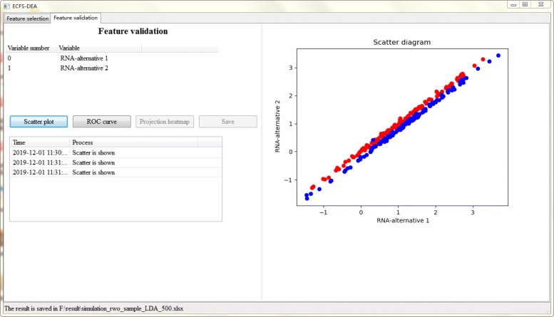
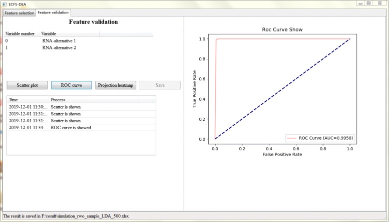
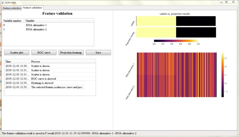
Figures 5, 6 and 7 together illustrate the panel for feature validation part of ECFS-DEA in Windows. Corresponding panels in Linux or Mac are almost the same. After pressing button “Scatter plot”, a 1-D, 2-D or 3-D scatter plot of the selected feature is shown in Fig. 5. Scatter plots with different colors denote samples from different groups. After pressing button “ROC curve”, the ROC curve of the selected feature is provided, as shown in Fig. 6. After pressing button “Projection heatmp”, the projection heatmap of the selected feature is presented, as shown in Fig. 7. A discrete projection from the expression levels of the selected feature (i.e., the classification results) is made. Samples are reordered according to the k-means clustering results of the projection values.
Fig. 5.
Feature validation step using a scatter plot in ECFS-DEA
Fig. 6.
Feature validation step using a ROC curve in ECFS-DEA
Fig. 7.
Feature validation step using a projection heatmap in ECFS-DEA
Detailed software documentation and tutorial are presented on http://bio-nefu.com/resource/ecfs-dea.
Results
Feature selection on the simulated data
In order to demonstrate the effectiveness of our ECFS-DEA, a simulated data consisting of 250 positive and 250 negative samples in a 40 dimensional space is constructed. 38 variables of them follow 38 normal distributions, each of which is independently and identically distributed and keeps a random mean value in range from 10 to 30 and a common standard deviation 0.01. The additional variable pair, i.e., miRNA-alternative 1 and miRNA-alternative 2, follows a bivariate normal distribution and has a clear category distinction. The mean vectors corresponding to positive and negative samples are (1,1)T and (1.11,0.89)T, respectively. Correspondingly, a same covariance matrix, which is expressed as , is kept.
We made this simulated data in order to show the effectiveness of using LDA compared to RF. Considering the comparability with real data, we made the sample size to be 500. This data can be downloaded at http://bio-nefu.com/resource/ecfs-dea.
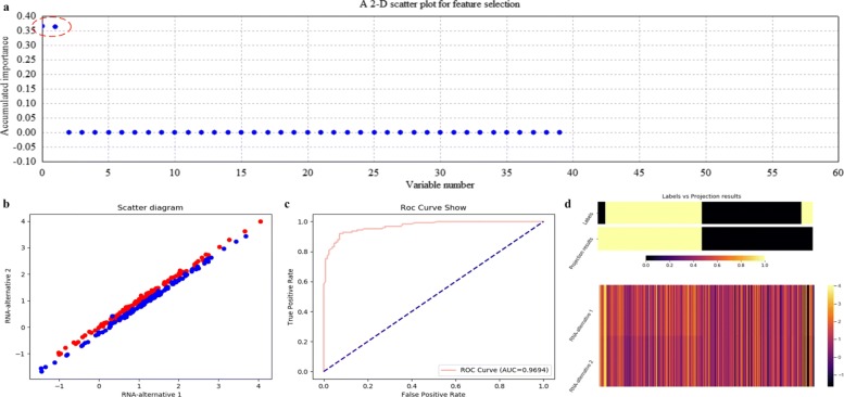
Using ECFS-DEA with LDA assigned as the base classifier, the significant variable pair is properly selected on the training set according to the accumulation of variable importance after 500 rounds of resampling, as shown in Fig. 8a. Meanwhile, the corresponding 2-D scatter plot, the ROC curve and the projection heatmap of the testing group are illustrated in turn, as shown in Fig. 8b, c and d. It can be seen in Fig. 8b that the testing set is 2-D but not 1-D linearly separable. The corresponding ROC curve is shown in Fig. 8c. As to Fig. 8d, a discrete projection from the expression levels of the selected variable pair (i.e., the classification results) is made. Samples are reordered according to the k-means cluster results of the projection values. It can be seen in Fig. 8d that a sample labeled 0 is misclassified, which corresponds to the blue point within the points labeled red in Fig. 8b.
Fig. 8.
Feature selection and validation on the simulated data using LDA. a Feature selection in a scatter plot form. b The 2-D scatter plot. c The ROC curve. d The projection heatmap
Figure 9 illustrates the variable selection results using kNN (k =5) on the simulated data after 500 rounds of resampling. In Fig. 9a, miRNA-alternative 1 and miRNA-alternative 2 are also intuitively selected. Correspondingly, the scatter plot, the ROC curve and the projection heatmap are listed in Fig. 9b, c and d, which show the effectiveness of choosing kNN as the base classifier on the simulated data.
Fig. 9.
Feature selection and validation on the simulated data using kNN (k=5). a Feature selection in a scatter plot form. b The 2-D scatter plot. c The ROC curve. d The projection heatmap
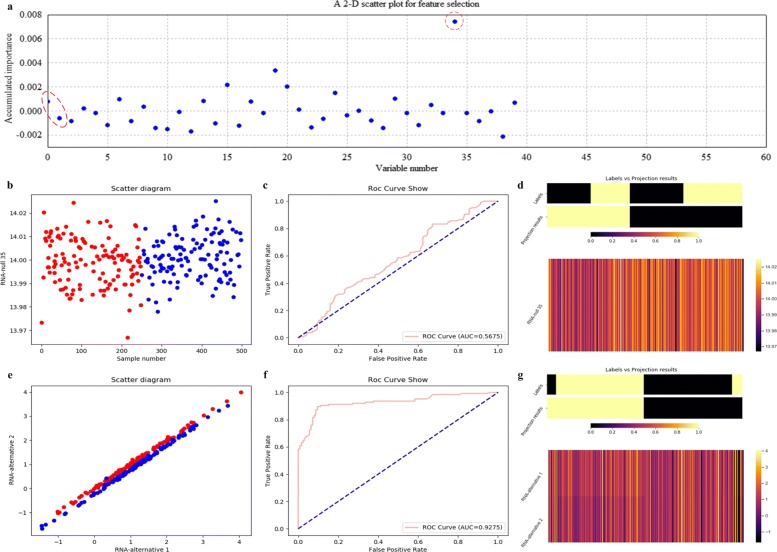
Figure 10 illustrates the variable selection results using RF on the simulated data after 500 rounds of resampling. As shown Fig. 10a, it is miRNA-null 35 but not miRNA-alternative 1 and miRNA-alternative 2 that is selected. And it is considered as a false selection. This directly demonstrates that RF is not applicable to any data with different sample distributions. Correspondingly, the scatter plot, the ROC curve and the projection heatmap of miRNA-null 35 are listed in Fig. 10b, c and d. All these results further demonstrate the above phenomenon.
Fig. 10.
Feature selection and validation on the simulated data using RF. a Feature selection in a scatter plot form. b The 1-D scatter plot of the selected feature with x and y coordinates to be sample indices and expression values. c The ROC curve of the selected feature. d The projection heatmap of the selected feature. e The 2-D scatter plot of the significant pair. f The ROC curve of the significant pair. g The projection heatmap of the significant pair
Figure 10b illustrates a 1-D scatter plot of the selected miRNA-null 35 using RF. The horizontal and vertical coordinates correspond to sample indices and expression levels, respectively. It can be seen that samples from two categories of the testing data are indivisible according to the vertical coordinate values. Figure 10c illustrates a poor ROC curve. As to Fig. 10d, it can be seen that the two clusters derived from the projection results contain many wrong labels.
Correspondingly, we also make the scatter plot, the ROC curve and the projection heatmap using RF on miRNA-alternative 1 and miRNA-alternative 2, which are listed in Fig. 10e, f and g, respectively. The experimental results of RF have improved; however, its ROC curve and projection heatmap are inferior to those of kNN and LDA.
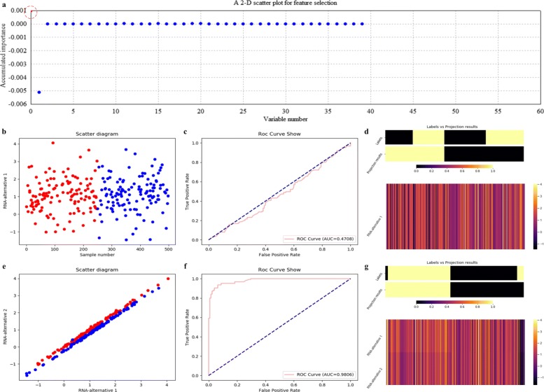
As to SVM which is assigned as the base classifier, it is only miRNA-alternative 1 but not the significant pair that is selected, as illustrated in Fig. 11a. It indicates that SVM is not applicable to the simulated data for feature selection. Correspondingly, the scatter plot, the ROC curve and the projection heatmap of miRNA-alternative 1 are listed in Fig. 11b, c and d. On the contrary, we also make the scatter plot, the ROC curve and the projection heatmap using SVM on miRNA-alternative 1 and miRNA-alternative 2, as shown in Fig. 11e, f and g.
Fig. 11.
Feature selection and validation on the simulated data using SVM. a Feature selection in a scatter plot form. b The 1-D scatter plot of the selected feature with x and y coordinates to be sample indices and expression values. c The ROC curve of the selected feature. d The projection heatmap of the selected feature. e The 2-D scatter plot of the significant pair. f The ROC curve of the significant pair. g The projection heatmap of the significant pair
The quantitative results on the simulated data with measures such as confusion matrix, precision, recall and F1-measure are listed in Table 1. In fact, it can be seen that RF and SVM achieve poor results, for they correspond to lower scores of accumulated importance compared with those of LDA and kNN, as shown in Figs. 8a, 9a, 10a and 11a, respectively. All the experimental results indicate that LDA is a more appropriate classifier for feature selection on the simulated data.
Table 1.
Quantitative results on the simulation data
| Base classifier | Variable number | Confusion matrix | Positive class | Precision | Recall | F1-measure | ||
|---|---|---|---|---|---|---|---|---|
| LDA | [0,1]T | classified as | a | b | a | 0.992 | 0.984 | 0.988 |
| label a | 123 | 2 | b | 0.984 | 0.992 | 0.988 | ||
| label b | 1 | 124 | weighted average | 0.988 | 0.988 | 0.988 | ||
| kNN | [0,1]T | classified as | a | b | a | 0.906 | 0.928 | 0.917 |
| label a | 116 | 9 | b | 0.926 | 0.904 | 0.915 | ||
| label b | 12 | 113 | weighted average | 0.916 | 0.916 | 0.916 | ||
| RF | 34 | classified as | a | b | a | 0.528 | 0.448 | 0.485 |
| label a | 56 | 69 | b | 0.521 | 0.600 | 0.558 | ||
| label b | 50 | 75 | weighted average | 0.524 | 0.524 | 0.522 | ||
| [0,1]T | classified as | a | b | a | 0.897 | 0.904 | 0.900 | |
| label a | 113 | 12 | b | 0.903 | 0.896 | 0.899 | ||
| label b | 13 | 112 | weighted average | 0.900 | 0.900 | 0.899 | ||
| SVM | 0 | classified as | a | b | a | 0.467 | 0.400 | 0.431 |
| label a | 50 | 75 | b | 0.476 | 0.544 | 0.508 | ||
| label b | 57 | 68 | weighted average | 0.472 | 0.472 | 0.470 | ||
| [0,1]T | classified as | a | b | a | 0.909 | 0.960 | 0.934 | |
| label a | 120 | 5 | b | 0.958 | 0.904 | 0.930 | ||
| label b | 12 | 113 | weighted average | 0.933 | 0.932 | 0.932 | ||
Feature selection on GSE22058
We also performed experiments on GSE22058 [29] which is a public dataset containing 96 samples associated with liver tumor and 96 samples corresponded to adjacent liver non-tumor. In order to achieve a predictive feature from the 220 miRNAs, we utilized ECFS-DEA on GSE22058, with the base classifier to be LDA, kNN, RF and SVM.
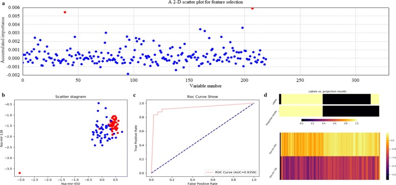
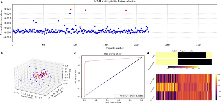
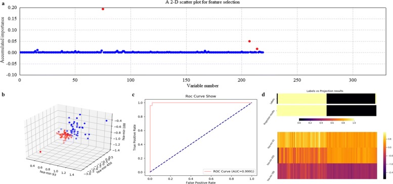
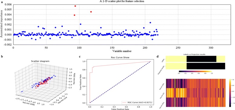
Figures 12, 13, 14 and 15 illustrate qualitative results for feature selection using LDA, kNN (k=5), RF and SVM on GSE22058 after 500 rounds of resampling, respectively. In order to exhibit the scatter plots at the feature validation step, we restricted feature dimension less than four. Besides, quantitative results on GSE22058 with measures such as confusion matrix, precision, recall and F1-measure are listed in Table 2, with all possible variables intuitively selected. All the experimental results indicate that RF is a more appropriate classifier to feature selection on GSE22058.
Fig. 12.
Feature selection and validation on GSE22058 using LDA. a Feature selection in a scatter plot form. b The 2-D scatter plot. c The ROC curve. d The projection heatmap
Fig. 13.
Feature selection and validation on GSE22058 using kNN (k=5). a Feature selection in a scatter plot form. b The 3-D scatter plot. c The ROC curve. d The projection heatmap
Fig. 14.
Feature selection and validation on GSE22058 using RF. a Feature selection in a scatter plot form. b The 3-D scatter plot. c The ROC curve. d The projection heatmap
Fig. 15.
Feature selection and validation on GSE22058 using SVM. a Feature selection in a scatter plot form. b The 3-D scatter plot. c The ROC curve. d The projection heatmap
Table 2.
Quantitative results on GSE22058
| Base classifier | Variable number | Confusion matrix | Positive class | Precision | Recall | F1-measure | ||
|---|---|---|---|---|---|---|---|---|
| LDA | 207 | classified as | a | b | a | 0.885 | 0.958 | 0.920 |
| label a | 46 | 2 | b | 0.955 | 0.875 | 0.913 | ||
| label b | 6 | 42 | weighted average | 0.920 | 0.916 | 0.917 | ||
| [207,38]T | classified as | a | b | a | 0.852 | 0.958 | 0.902 | |
| label a | 46 | 2 | b | 0.952 | 0.833 | 0.889 | ||
| label b | 8 | 40 | weighted average | 0.902 | 0.895 | 0.895 | ||
| [207,38,198]T | classified as | a | b | a | 0.887 | 0.979 | 0.931 | |
| label a | 47 | 1 | b | 0.977 | 0.875 | 0.923 | ||
| label b | 6 | 42 | weighted average | 0.932 | 0.927 | 0.927 | ||
| [207,38,198,160]T | classified as | a | b | a | 0.922 | 0.979 | 0.950 | |
| label a | 47 | 1 | b | 0.978 | 0.917 | 0.947 | ||
| label b | 4 | 44 | weighted average | 0.950 | 0.948 | 0.948 | ||
| [207,38,198, | classified as | a | b | a | 0.922 | 0.979 | 0.950 | |
| label a | 47 | 1 | b | 0.978 | 0.917 | 0.947 | ||
| 160,164]T | label b | 4 | 44 | weighted average | 0.950 | 0.948 | 0.948 | |
| [207,38,198, | classified as | a | b | a | 0.904 | 0.979 | 0.940 | |
| label a | 47 | 1 | b | 0.977 | 0.896 | 0.935 | ||
| 160,164,75]T | label b | 5 | 43 | weighted average | 0.941 | 0.938 | 0.938 | |
| kNN | 94 | classified as | a | b | a | 0.730 | 0.958 | 0.829 |
| label a | 46 | 2 | b | 0.939 | 0.646 | 0.765 | ||
| label b | 17 | 31 | weighted average | 0.835 | 0.802 | 0.797 | ||
| [94,118]T | classified as | a | b | a | 0.800 | 1.000 | 0.889 | |
| label a | 48 | 0 | b | 1.000 | 0.750 | 0.857 | ||
| label b | 12 | 36 | weighted average | 0.900 | 0.875 | 0.873 | ||
| [94,118,183]T | classified as | a | b | a | 0.828 | 1.000 | 0.906 | |
| label a | 48 | 0 | b | 1.000 | 0.792 | 0.884 | ||
| label b | 10 | 38 | weighted average | 0.914 | 0.896 | 0.895 | ||
| [94,118,183,93]T | classified as | a | b | a | 0.787 | 1.000 | 0.881 | |
| label a | 48 | 0 | b | 1.000 | 0.729 | 0.843 | ||
| label b | 13 | 35 | weighted average | 0.893 | 0.865 | 0.862 | ||
| RF | 75 | classified as | a | b | a | 0.904 | 0.979 | 0.940 |
| label a | 47 | 1 | b | 0.977 | 0.896 | 0.935 | ||
| label b | 5 | 43 | weighted average | 0.941 | 0.938 | 0.938 | ||
| [75,207]T | classified as | a | b | a | 0.979 | 0.979 | 0.979 | |
| label a | 47 | 1 | b | 0.979 | 0.979 | 0.979 | ||
| label b | 1 | 47 | weighted average | 0.979 | 0.979 | 0.979 | ||
| [75,207,214]T | classified as | a | b | a | 0.979 | 0.979 | 0.979 | |
| label a | 47 | 1 | b | 0.979 | 0.979 | 0.979 | ||
| label b | 1 | 47 | weighted average | 0.979 | 0.979 | 0.979 | ||
| [75,207,214,16]T | classified as | a | b | a | 0.980 | 1.000 | 0.990 | |
| label a | 48 | 0 | b | 1.000 | 0.979 | 0.989 | ||
| label b | 1 | 47 | weighted average | 0.990 | 0.990 | 0.990 | ||
| SVM | 94 | classified as | a | b | a | 0.746 | 0.979 | 0.847 |
| label a | 47 | 1 | b | 0.970 | 0.667 | 0.790 | ||
| label b | 16 | 32 | weighted average | 0.858 | 0.823 | 0.819 | ||
| [94,118]T | classified as | a | b | a | 0.787 | 1.000 | 0.881 | |
| label a | 48 | 0 | b | 1.000 | 0.729 | 0.843 | ||
| label b | 13 | 35 | weighted average | 0.893 | 0.865 | 0.862 | ||
| [94,118,93]T | classified as | a | b | a | 0.774 | 1.000 | 0.873 | |
| label a | 48 | 0 | b | 1.000 | 0.708 | 0.829 | ||
| label b | 14 | 34 | weighted average | 0.887 | 0.854 | 0.851 | ||
In addition, we searched the selected miRNAs using ECFS-DEA with RF to be the classifier, i.e., miR-188, miR-450 and miR-93, on Web of Science with keywords to be such as liver tumor, hepatocellular carcinoma and HCC. Both miR-188 and miR-93 have been reported to be relevant to liver tumor. In fact, miR-188 achieved higher scores than other miRNAs, as shown in Fig. 14a. The retrieved results of miR-188 [30, 31] have indirectly demonstrated the effectiveness of ECFS-DEA.
Conclusions
ECFS-DEA is a top-down classification-based tool for seeking predictive variables associated with different categories of samples on expression profiles. Other than prevailing differential expression analysis for class prediction, an ensemble classifier-based thought is proposed in this paper. According to accumulated scores of variable importance, LDA, kNN, RF or SVM can be rightly assigned and is suitable for different sample distributions. Qualitative and quantitative experimental results have demonstrated the effectiveness of ECFS-DEA.
Availability and requirements
Project name: ECFS-DEA Project home page: http://bio-nefu.com/resource/ecfs-deaOperating system(s): Linux, Windows, Mac Programming language: Python (≥ 3.5) License: GPLv3 Any restrictions to use by non-academics: none
Acknowledgements
Not applicable.
Abbreviations
- DEA
Differential expression analysis
- ECFS-DEA
Ensemble classifier-based feature selection for differential expression analysis
- JCD-DEA
Joint covariate detection for differential expression analysis
- kNN
k-nearest-neighbor
- LDA
Fisher’s linear discriminative analysis
- PBS
Portable batch system
- RF
Random forest
- ROC
Receiver operating characteristic
- SAM
Significance analysis of microarrays
Authors’ contributions
XDZ and GHW conceived the general project and supervised it. QJ, HYL and YMW were the principal developers. QJ and HYL developed the main graphical user interface parts. HXW made the supplementary experiments on the simulated data. YMW wrote the client-server connection related part and the software documentation. HYL and YMW built the server components. QJ developed the underlying source code. XDZ wrote the original manuscript. SH tested the software and made the revision on the manuscript. All authors read and approved the final manuscript.
Funding
This work has been supported by the financial support of Natural Science Foundation of China (No. 61771165), China Postdoctoral Science Foundation Funded Project (No. 2014M551246, 2018T110302), Innovation Project of State Key Laboratory of Tree Genetics and Breeding (Northeast Forestry University, No.2019A04), Fundamental Research Funds for the Central Universities (No. 2572018BH01), National Undergraduate Innovation Project (No. 201910225184) and Specialized Personnel Start-up Grant (Also National Construction Plan of World-class Universities and First-class Disciplines, No. 41113237). The funding body of Natural Science Foundation of China played an important role in the design of the study, collection, analysis and interpretation of data and in writing the manuscript.
Availability of data and materials
The public dataset analysed during the current study is available in the GEO repository. GSE22058 is available at https://www.ncbi.nlm.nih.gov/geo/query/acc.cgi?acc=GSE22058. The simulated data can be downloaded on http://bio-nefu.com/resource/ecfs-dea.
Ethics approval and consent to participate
Not applicable.
Consent for publication
Not applicable.
Competing interests
The authors declare that they have no competing interests.
Footnotes
Publisher’s Note
Springer Nature remains neutral with regard to jurisdictional claims in published maps and institutional affiliations.
The authors wish it to be known that, in their opinion, the first three authors should be regarded as Joint First Authors.
References
- 1.Lambrou GI, Sdraka M, Koutsouris D. The “Gene Cube”: a novel approach to three-dimensional clustering of gene expression data. Curr Bioinforma. 2019;14:721–7. doi: 10.2174/1574893614666190116170406. [DOI] [Google Scholar]
- 2.Storey John D., Tibshirani Robert. Statistics for Biology and Health. New York, NY: Springer New York; 2003. SAM Thresholding and False Discovery Rates for Detecting Differential Gene Expression in DNA Microarrays; pp. 272–290. [Google Scholar]
- 3.Ritchie ME, Phipson B, Wu D, Hu Y, Law CW, Shi W, Smyth GK. Limma powers differential expression analyses for RNA-sequencing and microarray studies. Nucleic Acids Res. 2015;43:e47. doi: 10.1093/nar/gkv007. [DOI] [PMC free article] [PubMed] [Google Scholar]
- 4.Pollard KS, Dudoit S, van der Laan MJ. Multiple testing procedures: the multiset package and application to genomics In: Gentleman R, Carey V, Huber W, Irizarry R, Dudoit S, editors. Bioinformatics and Computational Biology Solutions Using R and Bioconductor. Springer: 2005. p. 249–71. https://link.springer.com/chapter/10.1007%2F0-387-29362-0_15.
- 5.Zhao XD, Wang L, Chen GS. Joint covariate detection on expression profles for identifying microRNAs related to venous metastasis in hepatocellular carcinoma. Sci Rep. 2017;7:1–11. doi: 10.1038/s41598-016-0028-x. [DOI] [PMC free article] [PubMed] [Google Scholar]
- 6.Kanji GK. 100 statistical tests, 3rd edition: SAGE Publication; 2006. 10.4135/9781849208499.
- 7.Liu B, Gao X, Zhang H. BioSeq-Analysis2.0: an updated platform for analyzing DNA, RNA, and protein sequences at sequence level and residue level based on machine learning approaches. Nucleic Acids Res. 2019;47:e127. doi: 10.1093/nar/gkz740. [DOI] [PMC free article] [PubMed] [Google Scholar]
- 8.Lai HY, Zhang ZY, Su ZD, Su W, Ding H, Chen W, Lin H. iProEP: a computational predictor for predicting promoter. Mol Ther Nucleic Acids. 2019;17:337–46. doi: 10.1016/j.omtn.2019.05.028. [DOI] [PMC free article] [PubMed] [Google Scholar]
- 9.Lv H, Zhang ZM, Li SH, Tan JX, Chen W, Lin H. Evaluation of different computational methods on 5-methylcytosine sites identification. Brief Bioinforma. 2019; bbz048. https://academic.oup.com/bib/advance-articleabstract/doi/10.1093/bib/bbz048/5510088?redirectedFrom=fulltext. [DOI] [PubMed]
- 10.Zou Q, Xing PW, Wei LY, Liu B. Gene2vec: gene subsequence embedding for prediction of mammalian n6-methyladenosine sites from mRNA. RNA. 2019;25:205–18. doi: 10.1261/rna.069112.118. [DOI] [PMC free article] [PubMed] [Google Scholar]
- 11.Jia CZ, Zuo Y, Zou Q. O-GlcNAcPRED-II: an integrated classification algorithm for identifying O-GlcNAcylation sites based on fuzzy undersampling and a k-means PCA oversampling technique. Bioinformatics. 2018;34:2029–36. doi: 10.1093/bioinformatics/bty039. [DOI] [PubMed] [Google Scholar]
- 12.Li SH, Zhang J, Zhao YW, Dao FY, Ding H, Chen W, Tang H. iPhoPred: a predictor for identifying phosphorylation sites in human protein. IEEE Access. 2019;7:17–28. [Google Scholar]
- 13.Lv ZB, Jin SS, Ding H, Zou Q. A random forest sub-Golgi protein classifier optimized via dipeptide and amino acid composition features. Front Bioeng Biotechnol. 2019;7:215. doi: 10.3389/fbioe.2019.00215. [DOI] [PMC free article] [PubMed] [Google Scholar]
- 14.Zhu XJ, Feng CQ, Lai HY, Chen W, Lin H. Predicting protein structural classes for low-similarity sequences by evaluating different features. Knowl Based Syst. 2019;163:787–93. doi: 10.1016/j.knosys.2018.10.007. [DOI] [Google Scholar]
- 15.Ru XQ, Li LH, Zou Q. Incorporating distance-based top-n-gram and random forest to identify electron transport proteins. J Proteome Res. 2019;18:2931–9. doi: 10.1021/acs.jproteome.9b00250. [DOI] [PubMed] [Google Scholar]
- 16.Li YJ, Niu MT, Zou Q. ELM-MHC: an improved MHC identification method with extreme learning machine algorithm. J Proteome Res. 2019;18:1392–401. doi: 10.1021/acs.jproteome.9b00012. [DOI] [PubMed] [Google Scholar]
- 17.Li C, Liu B. MotifCNN-fold: protein fold recognition based on fold-specific features extracted by motif-based convolutional neural networks. Brief Bioinforma. 2019; bbz133. 10.1093/bib/bbz133. [DOI] [PubMed]
- 18.Liu B, Zhu Y, Yan K. Fold-LTR-TCP: protein fold recognition based on triadic closure principle. Brief Bioinforma. 2019; bbz139. 10.1093/bib/bbz139. [DOI] [PubMed]
- 19.Liu B, Li C, Yan K. DeepSVM-fold: Protein fold recognition by combining Support Vector Machines and pairwise sequence similarity scores generated by deep learning networks. Brief Bioinforma. 2019;bbz098. 10.1093/bib/bbz098. [DOI] [PubMed]
- 20.Song J, Wang H, Wang J, Leier A, Marquez-Lago T, Yang B, Zhang Z, Akutsu T, Webb GI, Daly RJ. PhosphoPredict: A bioinformatics tool for prediction of human kinase-specific phosphorylation substrates and sites by integrating heterogeneous feature selection. Sci Rep. 2017;7:6862. doi: 10.1038/s41598-017-07199-4. [DOI] [PMC free article] [PubMed] [Google Scholar]
- 21.Song J, Tan H, Boyd SE, Shen H, Mahmood K, Webb GI, Akutsu T, Whisstock JC, Pike RN. Bioinformatic approaches for predicting substrates of proteases. J Bioinforma Comput Biol. 2011;9:149–78. doi: 10.1142/S0219720011005288. [DOI] [PubMed] [Google Scholar]
- 22.Song J, Tan H, Wang M, Webb GI, Akutsu T. TANGLE: two-level support vector regression approach for protein backbone torsion angle prediction from primary sequences. PloS ONE. 2012;7:e30361. doi: 10.1371/journal.pone.0030361. [DOI] [PMC free article] [PubMed] [Google Scholar]
- 23.Cheng XP, Cai HM, Zhang Y, Xu B, Su WF. Optimal combination of feature selection and classification via local hyperplane based learning strategy. BMC Bioinformatics. 2015;16:219. doi: 10.1186/s12859-015-0629-6. [DOI] [PMC free article] [PubMed] [Google Scholar]
- 24.Cai HM, Ruan PY, Ng M, Akutsu T. Feature weight estimation for gene selection: a local hyperlinear learning approach. BMC Bioinformatics. 2014;15:70. doi: 10.1186/1471-2105-15-70. [DOI] [PMC free article] [PubMed] [Google Scholar]
- 25.Shmueli G. To Explain or to Predict? 2010; 25:289–311. 10.2139/ssrn.1351252.
- 26.Breiman L. Random forests. Mach Learn. 2001;45:5–32. doi: 10.1023/A:1010933404324. [DOI] [Google Scholar]
- 27.Lv ZB, Jin SS, Ding H, Zou Q. A random forest sub-Golgi protein classifier optimized via dipeptide and amino acid composition features. Front Bioeng Biotechnol. 2019;7:215. doi: 10.3389/fbioe.2019.00215. [DOI] [PMC free article] [PubMed] [Google Scholar]
- 28.Li Y, Liu YN, Wu YM, Zhao XD. JCD-DEA: a joint covariate detection tool for differential expression analysis on tumor expression profiles. BMC Bioinformatics. 2019;20:365. doi: 10.1186/s12859-019-2893-3. [DOI] [PMC free article] [PubMed] [Google Scholar]
- 29.Burchard J, Zhang C, Liu AM, Poon RT, Lee NPY, Wong KF, Sham PC, Lam BY, Ferguson MD, Tokiwa G, Smith R, Leeson B, Beard R, Lamb JR, Lim L, Mao M, Dai H, Luk JM. microRNA-122 as a regulator of mitochondrial metabolic gene network in hepatocellular carcinoma. Mol Syst Biol. 2010;24:402. doi: 10.1038/msb.2010.58. [DOI] [PMC free article] [PubMed] [Google Scholar]
- 30.Ma JC, Qin CY, Yuan ZG, Liu SL. LncRNA PAPAS promotes hepatocellular carcinoma by interacting with miR-188-5p. J Cell Biochem. 2019;120:13494–500. doi: 10.1002/jcb.28623. [DOI] [PubMed] [Google Scholar]
- 31.Meng FZ, Zhang SG, Song RP, Liu Y, Wang JB, Liang YJ, Wang JZ, Han JH, Song X, Lu ZY, Yang GC, Pan SH, Li XY, Liu YF, Zhou F, Wang Y, Cui YF, Zhang B, Ma K, Zhang CY, Sun YF, Xin MY, Liu LX. NCAPG2 overexpression promotes hepatocellular carcinoma proliferation and metastasis through activating the STAT3 and NF-kappa B/miR-188-3p pathways. Ebiomedicine. 2019;44:237–49. doi: 10.1016/j.ebiom.2019.05.053. [DOI] [PMC free article] [PubMed] [Google Scholar]
Associated Data
This section collects any data citations, data availability statements, or supplementary materials included in this article.
Data Availability Statement
The public dataset analysed during the current study is available in the GEO repository. GSE22058 is available at https://www.ncbi.nlm.nih.gov/geo/query/acc.cgi?acc=GSE22058. The simulated data can be downloaded on http://bio-nefu.com/resource/ecfs-dea.


