Understanding the Impacts of Short‐Term Climate Variability on Drinking Water Source Quality: Observations From Three Distinct Climatic Regions in Tanzania

Abstract

Climate change is expected to increase waterborne diseases especially in developing countries. However, we lack understanding of how different types of water sources (both improved and unimproved) are affected by climate change, and thus, where to prioritize future investments and improvements to maximize health outcomes. This is due to limited knowledge of the relationships between source water quality and the observed variability in climate conditions. To address this gap, a 20‐month observational study was conducted in Tanzania, aiming to understand how water quality changes at various types of sources due to short‐term climate variability. Nine rounds of microbiological water quality sampling were conducted for Escherichia coli and total coliforms, at three study sites within different climatic regions. Each round included approximately 233 samples from water sources and 632 samples from households. To identify relationships between water quality and short‐term climate variability, Bayesian hierarchical modeling was adopted, allowing these relationships to vary with source types and sampling regions to account for potentially different physical processes. Across water sources, increases in E. coli/total coliform levels were most closely related to increases in recent heavy rainfall. Our key recommendations to future longitudinal studies are (a) demonstrated value of high sampling frequency and temporal coverage (a minimum of 3 years) especially during wet seasons; (b) utility of the Bayesian hierarchical models to pool data from multiple sites while allowing for variations across space and water sources; and (c) importance of a multidisciplinary team approach with consistent commitment and sharing of knowledge.

Key Points

• We present a longitudinal study in a developing country on water quality changes at a range of water sources under climate variability

• Increases in E. coli and Total Coliform levels were most closely related to recent heavy rainfall

• Recommendations for future cross disciplinary studies on drinking water quality and relationships with climate variability are made

1. Introduction

Improved drinking water sources, including piped water to household, boreholes, protected dug wells, and rainwater, are effective ways to reduce human exposure to harmful waterborne bacteria and other pathogens, particularly in developing countries (Cairncross et al., 2010; Howard et al., 2010; Mills & Cumming, 2016; Wolf et al., 2014). In 2017, the Joint Monitoring Program estimated that 2.1 billion people do not have safely managed water services on premises, within which 537 million people still lack access to an improved water source; further, improved water sources are still vulnerable to fecal contamination, and it is estimated that at least 2 billion people use water sources that are fecally contaminated (WHO & UNICEF, 2017). Hence, developing countries are most prone to increasing risks of contamination and thus waterborne diseases due to climate change (Hashizume et al., 2007; Schijven & de Roda Husman, 2005; Singh et al., 2001; Smith et al., 2014; Taylor et al., 2009; Zhou et al., 2004). Therefore, it is vital to understand how climate change may affect water quality at various water sources. This will assist decision‐making for future investments on drinking water infrastructures to achieve the best health outcomes in the long term (Luh et al., 2017; Mellor et al., 2016).

Anthropogenic climate change is expected to impact water quality via multiple pathways, which involve complex biological and hydro‐climatic processes (Calow et al., 2011; Chigbu et al., 2004; Hales et al., 2003; Howard et al., 2010; Luh et al., 2017; Schijven & de Roda Husman, 2005; Vermeulen & Hofstra, 2014). The impacts of these processes are also known to vary across different natural water systems due to variations in geographic locations and baseline hydro‐climatic conditions (Döll & Flörke, 2005; Goderniaux et al., 2011; Macdonald et al., 2009). However, there are very few quantitative assessments on how source water quality may change with climate change. This is because there is not a wide understanding of even how water sources have historically responded to weather and climate variations (Howard et al., 2003; Levy et al., 2009; Sadik et al., 2017; Taylor et al., 2009; Wu et al., 2016). The main limitation of the existing studies is their limited spatial domain and, in some cases, the limited temporal sampling which hinders extrapolation of the results to a range of geographic and climate conditions. There is thus a clear gap in the literature on the relationship between climate variability and water quality derived from multiregion multiclimate studies. Without this baseline knowledge of current systems' behaviors, projection of anthropogenic climate change impacts remains difficult.

Tanzania has a particularly poor drinking water supply status, with improved drinking water accessible by only 76% of the country's total population (WHO & UNICEF, 2017). Analogies for the potential impacts of climate change on water supply sources and water‐related diseases in Tanzania can be found in historical climatically extreme periods. For example, between August 2015 and early 2017, a large cholera outbreak caused over 25,000 infections across 23 of the 25 regions across the country; the reported Case Fatality Rate ranged from 1.1% to 1.5% (McCrickard et al., 2017; Narra et al., 2017). This large‐scale outbreak was related to a strong El Niño weather pattern that brought heavy rains to East Africa (Narra et al., 2017). Climate change is expected to cause increases in temperature in Tanzania (Christensen et al., 2007) and further intensify existing extreme rainfall conditions (Shongwe et al., 2011; Vizy & Cook, 2012). Based on the El Niño experiences, this could be expected to affect water quality at supply sources and lead to detrimental effects on public health (GWP & UNICEF, 2014; Oates et al., 2014). However, further research is needed to quantitatively asses these potential impacts.

The observed vulnerability of water‐related public health to climate fluctuations highlights the need to advance the understanding of the relationships between source water quality and short‐term climate variability. In this paper, a suitable framework is presented to meet this need. The framework has been applied to a field‐based research study, which focused on longitudinal sampling and analyses of water quality and climate conditions over a 20‐month period, for three regions in Tanzania. This study is part of a larger research project led by the United Kingdom Department for Investment in Development and the World Health Organization (WHO) across four developing countries, titled “Building adaptation to climate change in health in least developed countries through resilient water, sanitation and hygiene.”

This paper begins with a comprehensive literature review, which covers current understanding of water quality at supply sources and how these can be affected by climate variability and change, focusing on the developing world (section 2). The literature review highlights the lack of quantitative understanding of relationships between source water quality and climate variability as a critical knowledge gap (section 3). A field‐based research protocol is then introduced, which highlights suitable methodologies to explore the relationship between climate variability and water quality at various sources in Tanzania. The sampling and analyses approaches are presented followed by key results, together with discussions on how these results can help understanding climate change impact on drinking water quality at the study locations (section 4). Based on experiences learned from the research, recommendations are made for enhanced study designs to link source water quality with climate variability (section 5).

2. Current Understanding of How Climate Change Can Impact Water Quality at Supply Sources

There are a number of fecal‐oral pathways for disease transmission (Figure 1). Waterborne diseases are transmitted when water contaminated by fecal material becomes a transmission pathway for fecal pathogens. The transmission to humans occurs through three main pathways: (1) consumption of drinking water; (2) consumption of food prepared using the water; and (3) contact of hands and other parts of the body with water during hygiene practices. Along these transmission pathways, improved water, sanitation and hygiene programs, and infrastructure, collectively referred to as WaSH, act as barriers to prevent the spread of waterborne diseases. These three components are often considered together, since the effectiveness of each component is dependent on one other. For example, without toilets, water sources become contaminated; without clean water, basic hygiene practices are not possible (UNICEF, 2016).

Figure 1.

Illustration of how diseases are transmitted via fecal‐oral routes (arrows) and how WaSH act as barriers (dashed lines) for these transmission routes. Note that only the waterborne pathway (highlighted in orange) is the focus of this study, and other pathways (colored in gray) are not discussed. Figure adapted from Water1st International (2017).

The primary factors that differentiate the water quality at supply sources are the infrastructure (e.g., channels and pipelines) and technology (e.g., disinfection) that are used to improve public health. Based on these features, the WHO/UNICEF Joint Monitoring Program for WaSH has established broad categories to summarize the relative effectiveness of different types interventions for each of the water, sanitation, and hygiene sectors (WHO & UNICEF, 2017). The drinking water supply categories are mainly focused on the types of water sources, as well as the time taken for water collection. Improved interventions are characterized by water sources with protective infrastructure (such as lids or pipes).

The effectiveness of improved water sources has been confirmed with several analytical studies of observed water quality, often represented by the presence of fecal indicator bacteria (FIB) in water. Bain, Cronk, Hossain, et al. (2014) systematically reviewed 345 water quality observational studies for the probability of FIB contamination across various water sources, for multiple regions around the world. Overall, these studies suggested that boreholes were more frequently contaminated than piped water, with 10% to 41% increases in the proportion of contaminated samples. In addition, contamination was identified for the vast majority of samples collected at unprotected groundwater sources. In a later review of 319 studies, the average risks of FIB contamination in water from an improved source were estimated to be only 15% of that for unimproved sources (Bain, Cronk, Wright, et al., 2014). Another meta‐analysis also summarized the fecal contamination reported in 45 studies, which suggested that at a source level, the average contamination risk at pipes is only 20% of that of the nonpiped sources (Shields et al., 2015).

It is difficult to extrapolate these findings to consider how contamination may change due to anthropogenic climate change. This is because, to date, most climate change assessments on water quality have been largely limited to investigating the impacts on natural freshwater systems such as streams, lakes, and groundwater aquifers. Expected climatic changes include increases in extreme rainfall and floods (Wasko & Sharma, 2017; Westra et al., 2014), as well as prolonged and more frequent droughts (Prudhomme et al., 2014). All of these hydroclimatic events can affect both the quantity and quality of water within natural and engineered water systems, which thus affect the mobilization and transportation processes of contaminants that enter into water sources. Specifically, these impacts can propagate via three main categories of processes (Howard et al., 2010; Oates et al., 2014):

• Changes in quantity of available freshwater resources, which can affect the quality of drinking water supply through the dilution and/or transportation of contaminants;

• Intensification of extreme events and natural disasters, which can affect the performance and reliability of water supply infrastructures (e.g., dams and pipes); and

• Shifts in biological and hydrological processes in response to changing climate conditions, which can lead to changes in contamination risks for drinking water sources.

These major physical processes through which climate change can impact freshwater systems and thus drinking water quality are summarized in Figure 2 with more detailed discussed in the subsequent sections. These discussions focus specifically on water contamination from fecal pathogens in developing regions and countries.

Figure 2.

Major physical processes through which climate change can impact natural freshwater systems, as represented by red arrows and texts. Colored boxes highlight various types of water supply sources. Brown block arrows represent possible sources of fecal pathogens, and presence of these pathogens are shown in black asterisks. This figure focuses on common processes seen in developing regions and countries.

Climate change is expected to cause changes in rainfall and runoff in different ways across the main regions of the developing world. Although future rainfall projections for Asia are largely uncertain, it is more confident that by the end of 21st century, Northern Africa and the southwestern parts of South Africa are expected to experience reduction in rainfall, while likely increases of rainfall are expected in regions of high or complex topography such as the Ethiopian Highlands (Hijioka et al., 2014; Niang et al., 2014). For regions that will experience decreasing rainfall, drinking water sources are likely undersupplied and/or having only intermittent supply (Calow et al., 2011; Howard et al., 2010; Oates et al., 2014; WHO & UNICEF, 2017). Expected increases in temperature can lead to higher evapotranspiration, which places further stress on water supplies. Increases in flooding events can be following by outbreaks of cholera, typhoid, and diarrhea due to possible contamination of floodwaters by human or animal waste. Drought reduces the water available for hygiene and sanitation, which thus also increases the risk of disease (Hales et al., 2003). Furthermore, the increasing frequency of climate extremes, such as floods, droughts, and heat waves, are more likely to disrupt the normal working conditions for water supply sources and even damage infrastructure such as pipes and water tanks (Calow et al., 2011; Howard et al., 2010; Luh et al., 2017).

Climate change can impact the biological and hydrological processes within natural water systems, which in turn affect the pathogen and bacteria levels in freshwater resources used as water sources. A changing climate can directly influence the biological cycle of fecal pathogens by modifying their growth and die‐off rates. In specific, higher inactivation rates are related to increasing temperature for both Escherichia coli (Schijven & de Roda Husman, 2005; Vermeulen & Hofstra, 2014) and fecal coliform (Chigbu et al., 2004).

Shifts in weather patterns can also impact the transport of fecal pathogens through hydrological processes (Luh et al., 2017; Smith et al., 2014). Within natural surface water systems, increases in precipitation and specifically extreme precipitation lead to higher risks of contaminant overflows, manure wash‐off and sediment erosion, and thus cause higher concentrations of fecal pathogens (e.g., Pednekar et al., 2005; Vermeulen & Hofstra, 2014). On the other hand, it has been found that increasing precipitation can also lead to a decrease in fecal pathogen concentration via dilution (Levy et al., 2009). The same mechanism also implies that if dry periods increase in length, higher fecal pathogen concentrations in surface water may result (Mellor et al., 2016; Wilby et al., 2005). Furthermore, more intense extreme precipitation can increase the turbulence in surface water, which increases the chance of fecal pathogen resuspension (Hofstra, 2011; Wu et al., 2009). In shallow, ephemeral groundwater systems that respond rapidly to rainfall recharge, elevated fecal pathogen levels were observed immediately following higher rainfall (Taylor et al., 2009), as well as during wet periods (Howard et al., 2003), which are likely related to the inflow of stagnant surface water and fecal materials from upstream.

The impacts of climate change will vary for different natural water systems, due to variations in geographic locations and baseline hydro‐climatic conditions of these systems. For example, the biological cycle of fecal pathogens can differ across aquatic systems. The reaction and transport of fecal pathogens can also be driven by different geographic and hydro‐climatic processes in different regions and during different times of a year. Systems fed by surface water in mountainous regions can be heavily affected by changes in rainfall patterns, via processes such as erosion and wash‐off during wet seasons and after heavy rains. In contrast, deep aquifers are generally buffered by large volume of storage and are thus less vulnerable to climate variability (Döll & Flörke, 2005; Goderniaux et al., 2011; Macdonald et al., 2009).

3. What Are the Gaps in Assessing Climate Change Impacts on Water Supply Sources?

Water quality at different supply sources is highly dependent on the infrastructure and technology employed. Climate change has the potential to substantially impact these “baseline” performances, via the complicated processes discussed above. However, quantitatively assessing these impacts is currently largely limited due to a lack of understanding of how source water quality has been affected by historical climate variability. Only a few studies have investigated these relationships, which are summarized in Table 1.

Table 1.

Existing Investigations on the Relationship Between Climate Variability and Source Water Quality

Source	Type(s) of drinking water sources	Changes in climatic features	Other factors	Spatial extent	Temporal extent	Analytical method	Findings
Howard et al. (2003)	Single type (protected springs)	Rainfall	Populationand on‐site sanitation practices	Single site (Kampala, Uganda)	Mar 1998 to Apr 1999	Multivariate regression with water quality classification derived from monitored data	Increasing microbiological contamination (thermotolerant coliforms and fecal streptococci) with rapid recharge of the springs after rainfall.
							Sources of feces such as waste dumps and drains appeared to be more significant than latrines.
Levy et al. (2009)	Multiple types (Unimproved surface water, rainwater, and unprotected dug wells [source and household levels])	Rainfall	Storage and treatment at household	Single site (Colon Eloy, Ecuador)	Jan 2005 to Mar 2006	Multivariate regression with monitored data	E. coli counts were generally higher in the wet season, with 0.42 and 0.11 log differences for source and household, respectively.
							In the wet season, a 1‐cm increase in weekly rainfall was associated with a 3% decrease in E. coli in source samples and a 6% decrease in household samples.
Taylor et al. (2009)	Single type (protected spring)	Heavy rain events	—	Single site (Kampala, Uganda)	July–Sep 2004	Visualizing inspection of trends and relationship in monitored data	Increasing contamination by thermotolerant coliforms in response to heavy rainfall events (>10 mm/day) during the rainy season.
Wu et al. (2016)	Single type (shallow tubewell)	Daily temp, daily rain, number of previous heavy rain days, and number of previous hot days	Land use and population	Multiple sites (MatlaChar and Char Para regions in Bangladesh)	May 2008 to Oct 2009	Multivariate regression with monitored data	E. coli presence was significantly associated with the number of heavy rain days (upper tenth percentile), developed land and regions with larger areas of surface water bodies (risk ratios 1.38, 1.07, and 1.02).
Sadik et al. (2017)	Multiple types (protected spring, public tap, drainage channel, and surface water)	Wet/dry seasons	—	Single site (Kampala, Uganda)	Nov 2014 to May 2015	t test for differences in monitored data from different seasons	Wet period is associated with higher presence of pathogenic genes including enterohemorrhagic E. coli, Shigella spp., Salmonella spp., Vibrio cholerae, and enterovirus
							Drainage channel and surface water contain higher pathogen levels compared with protected spring and public tap.

Note. The shaded cells indicate various influencing factors for source water quality.

All studies listed in Table 1 were based on FIB levels in water samples to assess drinking water quality. Although these studies were conducted for different spatial‐temporal extents and focused on different types of drinking water sources, one consistent finding from them is that higher concentrations of FIB are associated with wet periods and heavy rainfall. However, only three of the studies have quantified the impacts of rainfall variation as changes in presence or concentration of FIB, via multivariate regression models (Howard et al., 2003; Levy et al., 2009; Wu et al., 2016). The other studies were unable to explicitly quantify the impact of rainfall variation on water quality. Specifically, Taylor et al. (2009) visually examined the temporal trends in high‐frequency rainfall and water quality data, while Sadik et al. (2017) used significance tests to assess water quality differences between dry and wet periods. Therefore, it is difficult to predict water quality changes based on climate variability, which is a critical first step in making climate change projections for source water quality.

A greater and more general limitation in existing studies is the small number of combinations of climate features and types of water source, which limits the transferability of the results. Wu et al. (2016) considered a number of different types of climate variability, but only one type of water source is considered. Levy et al. (2009) and Sadik et al. (2017) included multiple types of water sources but only considered the impact of rainfall seasonality. Apart from Wu et al. (2016), each of the studies focused on a single study area, so their results are likely highly specific to the local/regional geographic and hydro‐climatic conditions. As such, it is not clear how these climatic impacts vary across different types of water source as well as different geographic and hydro‐climatic regions.

A framework is now presented that addresses both these gaps.

4. Closing the Gap: Research to Quantifying the Impacts of Climate Variability on Water Source Quality in Tanzania

4.1. Background

Targeting the knowledge gaps highlighted in section 3, in 2013, the United Kingdom Department for International Development funded a research project titled “Building adaptation to climate change in health in least developed countries through resilient water, sanitation and hygiene.” This project was managed by WHO, which initiated individual research projects at four developing countries: Bangladesh, Nepal, Ethiopia, and Tanzania. The findings from this study will be useful to assist decision‐makers to prioritize different WaSH interventions. Furthermore, these study designs are also transferable templates for other developing and developed countries to improve the understanding factors affecting WaSH effectiveness.

The Tanzania research aimed to explain how water quality at common water supply sources in Tanzania varies for a range of climate conditions in three different regions. To achieve this, the study focused on assessing drinking water quality, as represented by levels of FIB specifically E. coli and total coliforms (TCs) at drinking water supply sources and at households. It is noted that while E. coli has been widely accepted as FIB, TC can come from plants and soil and thus may not sufficient to identify fecal contamination. However, TC is still able to reflect the cleanliness of drinking water and has thus been recommended as an indicator of drinking water contamination where data are scarce, particularly for developing countries (WHO & UNICEF, 2017). An alternative measure of public health outcomes for water sources is the diarrhea morbidity, however, such epidemiological evidences have two key limitations: (1) biases due to unreported cases and (2) uncertainties from additional pathways besides waterborne transmission that are less relevant to assessing the effectiveness of water sources responses to climatic disturbance (e.g., infection through contaminated food and flies; Bain, Cronk, Hossain, et al., 2014; Hofstra, 2011). Therefore, we did not sample epidemiological evidences for assessing water quality.

To isolate different influencing factors for source water quality, structured sampling and data analyses schemes have been implemented. Household use surveys were also undertaken. This has been the first attempt in East Africa to undertake a study specifically designed to investigate the impact of climate variability on the effectiveness of water supply sources in such a systematic manner. The contributions of this study are the size and duration of the sampling campaigns as well as the temporal and spatial variability that was sampled. This approach, key findings, and implications of the research are summarized in the subsequent sections.

4.2. Sampling Scheme

Water quality monitoring was conducted in three study regions within Tanzania, namely, Buguruni, Kilombero, and Kondoa (Figure 3). These regions were selected to represent contrasting geographic features and climatic conditions, as well as a range of development contexts. Buguruni is a ward within the capital city of Dar es Salaam and is an informal urban community. The site has a wet coastal climate that is representative of the narrow eastern region in Tanzania. The Kilombero area is located in the southeastern highland of Tanzania with a mixed establishment of village communities. The region represents the very wet climate of the wetland valley areas. Lastly, the northern dry region is represented by the Kondoa region, which is also predominantly occupied by village communities.

Figure 3.

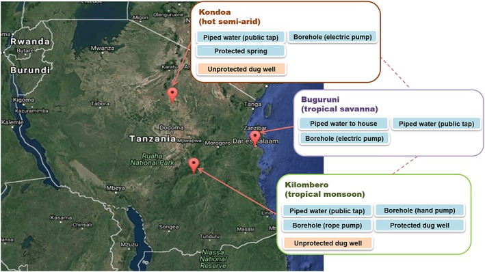
Schematic of the hierarchical water quality sampling for the Tanzania study. Within each study region, types of drinking water sources sampled are classified by improved (blue) and unimproved (orange) sources.

The study design was a longitudinal cohort observational study of existing drinking water source interventions across the three different climate regions. The study was multilevel with the sampling units being the different water sources (source level) and the individual household (household level). The dependent variable measured was water quality as E. coli and TC counts (both in colony‐forming units per 100 ml) in samples. Sampling was clustered geographically based on water source distribution (Figure 3). In addition to water quality observations, longitudinal surveys were also conducted to assess the WaSH practices and community health in each study region (not reported here).

For water quality sampling, water points were selected based on the common types within the region and reflected both improved and unimproved sources. The household‐level sampling points were randomly selected from all known households that rely on each water point. This selection process identified 90 water points in Buguruni, which consisted of borehole electric pump, piped water to house, and piped water (public tap; Table 2). Buguruni is the only sampled region where piped water is regularly chlorinated, which is supplied by the Utility (Dar es Salaam Water and Sewerage Corporation) or from private bores where chlorine dosing occurs in header tanks. The chlorine residuals were generally low (average 0.05 mg/L and not exceeding 0.92 mg/L) and, however, would have provided a disinfection residual for the water source. Buguruni has no unimproved water source because the majority of them were destroyed due to the previous cholera outbreak which occurred in 2015. A total of 240 households was selected from users of the sampled water points. Sampling within Kilombero consisted of 89 selected water points and 200 households, which covered improved water sources of borehole (hand pump and rope pump), piped water (public tap), and protected dug wells (pump). Unprotected dug wells, as a common unimproved water source in the region, were also included. The Kondoa region was sampled by considering 59 water points and 200 households. Improved water sources sampled within Kondoa included borehole (electric pump), piped water (public tap), and protected springs. Unimproved water sources were mainly shallow unprotected dug wells, which are located on river beds and mostly with an approximate depth of 1 m. Study sample sizes were calculated with a power to detect mean differences in water quality between sample types. As the study was multilevel, power calculations were made for both the household and community levels. The effects of clustering were considered in sample size calculations (Hemming et al., 2011). For each site, the calculated sample sizes were increased by 20% to account for loss to follow‐up during the longitudinal study.

Table 2.

Number of Water Points and Households at Which Water Quality Was Over Monitoring Period, Within Each Study Region

Type of WaSH intervention	Buguruni	Kilombero	Kondoa	Total water source
Source‐level sampling
Piped water to house	38	—	—	38
Piped water (public tap)	37	6	13	56
Borehole (electric pump)	15	—	15	30
Borehole (hand pump)	—	36	—	36
Borehole (rope pump)	—	5	—	5
Protected dug well	—	38	—	38
Protected spring	—	—	2	2
Unprotected dug well	—	4	29	33
Total water source	90	89	59	238
Household‐level sampling
Piped water to house	125 (12 networks)	—	—	125
Piped water (public tap)	54 (15 networks)	60 (6 networks)	60 (3 source)	174
Borehole (electric pump)	61 (6 networks)	—	60 (3 source)	121
Borehole hand pump	—	40 (2 source)	—	40
Borehole rope pump	—	20 (1 source)	—	20
Protected dug well	—	60 (5 source)	—	60
Unprotected dug well	—	20 (4 source)	80 (4 source)	100
Total households	240	200	200	640

Note. WaSH = water, sanitation and hygiene programs and infrastructure.

Water samples were collected in sterile 500‐ml bottles directly from the community water sources in duplicate. For taps and boreholes, water samples were assumed to be stable after 1 min of flushing. For households, the samples were collected from a household tap or storage vessel (bucket or water container). Water samples were cold‐chain transported to the laboratory and analyzed within 24 hr. Microbiological water testing for E. coli and TC was completed using the United States Environmental Protection Agency (US EPA) membrane filtration method 10029 with m‐ColiBlue24® Broth (Hach Company, 2016). ColiBlue24® is a single‐step membrane filtration procedure that incorporates specific noncoliform growth inhibitors and a selective enzymatic indicator to allow for simultaneous detection and quantitation of both E. coli and TCs. A water sample is filtered through a 0.45‐μm membrane filter and then placed in a petri dish containing a filter pad and mColiBlue24® nutrient broth and incubated at 37 °C ± 0.5 °C for 18 to 24 hr. Blue colonies are enumerated as E. coli, and red colonies are enumerated as TCs.

The wet season in the north and east of Tanzania consists of the “short rains” (October–December) and “long rains” (April to May). In the southern, western, and central areas, there is one long wet season (October–May). To ensure coverage of a wide range of climate conditions, the monitoring was conducted over a 20‐month period from July 2016 to February 2018. Within the study period, water quality sampling and household surveys were carried out in each study region every 2 months and was designed to capture the seasonal climatic cycle (Figure 4). Meteorological conditions, including rainfall, temperature, and relative humidity, were recorded daily by weather stations at both Kilombero and Kondoa sites. For Buguruni, no weather station data is accessible, so the National Oceanic and Atmoshperic Administration (NOAA) Global Historical Climate Network (GHCN)‐Daily station observations (Menne et al., 2012) were obtained for temperature and rainfall. In addition, the following two long‐term rainfall data sets were also obtained and will be used to understand how well the study period could represent long‐term conditions and to inform how the study results could be extrapolated to assess future climate change impacts (section 4.4):

1. Daily gridded rainfall data set of the Africa Rainfall Climatology 2 (Novella & Thiaw, 2013); and

2. Monthly historical observations requested from Tanzania meteorological agency.

Figure 4.

Water quality sampling schedule relative to seasonal climatic cycle of daily temperature (top row, gray lines show daily maximum and minimum temperature) and rainfall (bottom row) at three study locations during the study period. Red dots indicate dates when water quality samples were taken.

4.3. Data Analyses

The objective of the analyses was to determine the effects of short‐term climate variability on water quality and how these effects vary across different types of water sources within different climate regions in Tanzania. Bayesian hierarchical modeling (Gelman et al., 2013) was adopted in analyzing the relationships between water quality and climate data. The hierarchical structure allows these relationships to vary at different types of water sources and sampling regions and thus account for possible differences in physical processes that affect water quality. Bayesian hierarchical models are useful to analyze data that have clear grouping structures, especially when data for individual groups are limited (Borsuk et al., 2001; Webb et al., 2010). For this study the hierarchy was across the sampling regions and water source types. By calibrating the model with the entire data set, more robust estimates of relationships at individual water sources and sampling regions are obtained.

The water quality indicators (i.e., E. coli and TC) can both take zero values, which correspond to occasions where no contamination is detected in the water sample. Our analyses focused on explaining the variation of the nonzero counts for E. coli (TC) with separate modeling used to explain the occurrence of E. coli. The E. coli (TC) counts were categorized into i = 1, 2, 3 … m sampling groups with each group representing one unique combination of source type and study region. It was assumed that each group has a baseline water quality condition, defined by the mean value of the counts for the detected E. coli (TC). The temporal variations in water quality were modeled for each of j = 1, 2, 3 … n individual sampling dates. Thus, the model focuses on explaining the relationship between climate data and the variation of water quality around the relevant baseline mean for each sampling group. A Box‐Cox transformation was used to ensure that the E. coli (TC) counts were approximately normal, with Box‐Cox transformation parameters of 0.02 for E. coli and 0.20 for TC. The E. coli (TC) count in group i at any sampling date j, C_ij, was then drawn from a normal distribution with a mean μ_ij and the observed standard deviation σ _{i_obs} for the specific group (equation (1)). This structure accounts for random variation across multiple samples collected on the same day from the same group. The expected value of E. coli (TC) counts on the day, μ_ij, was modeled using the group‐level mean count, $\overline{C_{i¯\mathrm{obs}}}$, and a shift from the group‐level mean on the sampling date j, ∆_ij (equation (2)). This shift was modeled as a linear combination of n climatic predictors, X₁ to X_n which represent the effects of climate variability (equation (3)).

$$C_{\mathit{ij}}\sim N\left({\mu }_{\mathit{ij}},{\sigma }_{i\_\mathrm{obs}}\right).$$ (1)

$${\mu }_{\mathit{ij}}=\overline{C_{i\_\mathrm{obs}}}+{∆}_{\mathit{ij}}.$$ (2)

$${∆}_{\mathit{ij}}={\beta }_{1,i}\times X_{1,\mathit{ij}}+\cdots +{\beta }_{n,i}\times X_{n,\mathit{ij}}.$$ (3)

β_1,i to β_n,i represent the best‐fit parameters for the linear regression for group i, for the corresponding climatic predictors X₁ to X_n.

An “exhaustive search” process (Guyon & Elisseeff, 2003; May et al., 2011) was used to identify the best set of climatic predictors in the hierarchical models for E. coli/TC from all possible combinations. A wide range of potential predictors was selected that could explain the temporal variations in water quality, based on a review of existing literature (Curriero et al., 2001; Hofstra, 2011; Howard et al., 2003; Richardson et al., 2009; Taylor et al., 2009; Wu et al., 2016; Zhou et al., 2004). These potential predictors summarized various features of short‐term variability in rainfall and temperature which have been identified as the key influencing factors of FIB species in previous studies.

Rainfall on the same day as the water quality sampling (P) and rainfall on the preceding day (P_lag1) were both included as potential predictors to represent any immediate runoff effects on water quality. The number of dry days (rainfall <0.1 mm) and number of heavy rainfall events (daily rainfall >10 mm) during the 14 days prior to water quality sampling (drysp and P10_lag, respectively) were included to represent the inherent memory in water resources systems. The time window of 14 days was selected to maximize the correlation of the rainfall predictors with the water quality data based on preliminary analysis. Drinking water quality can also be affected by extremes that differ from long‐term average climate conditions, (e.g., Khan et al., 2015; Wu et al., 2016). The Standardized Precipitation Index (SPI) measures how much wetter or drier any particular month is compared to normal conditions at that time of year. The monthly SPIs were calculated by comparing each month within the study period with long‐term rainfall data (as per Hayes et al., 2011). For temperature, both the instantaneous and accumulated effects were considered with the maximum and minimum temperature on the day of water quality sampling (Tmax and Tmin, respectively) and the average daily temperature over 30 days preceding the sampling date (Ta_lag30). A total of eight climatic predictors was considered to start the exhaustive search, as summarized in Table 3.

Table 3.

Eight Potential Climatic Predictors to Model the Detection and Counts of E. coli and Total Coliform

Climatic predictors and units	Definition
P (mm)	Daily rainfall
P_lag1(mm)	Rainfall on the previous day
drysp (day)	Dry spell length: number of consecutive dry days (rainfall <0.1 mm) in past 14 days
P10_lag (day)	Number of heavy‐rain days (rainfall >10 mm) in past 14 days
SPI	The Standardized Precipitation Index which measures how much wetter or drier the month is compared to normal conditions at that time of year
Tmax (°C)	Daily maximum temperature
Tmin (°C)	Daily minimum temperature
Ta_lag30 (°C)	Average temperature over the past 30 days

The exhaustive search was performed by fitting a regression between each combination of predictors and the temporal variability in water quality. Note that although the hierarchical model structure allowed varying regression parameters across sampling groups (as equation (3)), during the search process, only a single value for each parameter (i.e., no variation across groups) was used to reduce the computational overhead. The Akaike (1974) information criterion was used to find the best combination of predictors that provides acceptable model performance while minimizing model complexity to avoid overfitting.

Once the best sets of climatic predictors were identified, the hierarchical models were fitted using the R package rstan (Stan Development Team, 2018). The fitting process used a Bayesian approach, in which each model parameter was sampled from a predefined prior distribution. The Bayesian approach combines these prior distributions with the recorded data samples to estimate the posterior distribution which represents the parameter values that maximize the likelihood of observed data. Noninformative priors were used in all cases. The fitted posterior model parameters provide information on the relative magnitude and direction of variations in each climatic predictor on E. coli and TC, across different sampling groups.

4.4. Key Results and Implications on Climate Change Impacts

Within the water quality monitoring data, clear differences have been observed between the source‐ and household‐level concentrations for both E. coli and TC with much higher concentrations observed in households (Figure 5). Household samples also have much weaker seasonal patterns suggesting little benefit in trying to explain water quality variations due to climate variability. Therefore, the modeling of relationships between climate variability and water quality focuses on the samples collected from water sources. For all regions, the improved water sources, namely, piped water and bores, have the best water quality. Unimproved sources (e.g., dug wells) have the poorest water quality.

Figure 5.

Variations in the detected counts in (a) average E. coli and (b) average TC across different types of water source and sampling seasons. To assist identification of temporal variations, both quantities are presented in a Box‐Cox transformed scale. Individual rows are used to distinguish samples obtained at water sources and households, whereas each column corresponds to each of the three study regions. TC = total coliform.

The key predictors for both E. coli and TC were found to include the number of heavy‐rain days over the preceding 14 days (P10_lag), the SPI of the previous month, and the daily minimum temperature (Tmin). TC has two additional predictors as the rainfall on the previous day (P_lag1) and the daily maximum temperature (Tmax). From the calibration of hierarchical model between climate variability and source water quality, it was found that the SPI has clear positive effects on both E. coli and TC for most regions and types of water sources (Figure 6). If a month is wetter compared to the long‐term average condition for that month (higher SPI), water quality in the following month is expected to be worse than the mean levels, for all sampling groups. Although of smaller magnitudes in general, P10_lag also has positive effects. These suggests that rainfall can have a “delayed” effect on source water quality over several days to weeks following rainfall, possibly via processes such as soil erosion and transport from upstream and groundwater replenishment. Tmin has clear positive influence on E. coli for most regions and sources, with higher magnitudes for Kilombero and Kondoa. Water sources in Buguruni, which are largely improved, are generally less affected by climate variability than Kilombero and Kondoa, with generally smaller effects of all climate predictors on both E. coli and TC counts across all types of water sources.

Figure 6.

Effects of the key climatic predictors for the counts of E. coli and TC, as the calibrated parameters of the Bayesian hierarchical models. Colored dots represent means, while gray bars represent parameter uncertainties by 95% confidence interval of the posterior distributions. Numbers following sampling group names indicate the number of detected data points within each sampling group. Shading highlights three distinct study locations. Note: All climatic predictors were transformed and standardized during the modeling process, so the magnitudes of their effects are indicative of the relative importance of each climatic parameter. TC = total coliform; SPI = Standardized Precipitation Index.

The positive impacts of heavy rainfall (represented by SPI and P10_lag) are consistent with previous findings that recent heavy precipitation events can lead to higher risks of fecal pathogen contamination both in surface water and groundwater sources, possibly due to (1) manure wash‐off and sediment erosion (Pednekar et al., 2005; Vermeulen & Hofstra, 2014); (2) increasing turbulence and thus the chance of pathogen resuspension (Hofstra, 2011; Wu et al., 2009); and (3) groundwater recharges with stagnant surface water and fecal materials from upstream (Howard et al., 2003; Taylor et al., 2009). By the mid‐21st century, Eastern Africa is expected to have wetter wet seasons, with projected increases in both heavy rainfall intensity (Seneviratne et al., 2012; Shongwe et al., 2011) and the number of extreme wet days (Vizy & Cook, 2012) over the region. Therefore, the effects of heavy rainfall on source water quality identified in this study suggest potential of future deterioration of drinking water quality in the study regions.

The framework demonstrated in this study enables quantitative projections of future water quality at various sources across the study locations. To achieve this, two key steps would be required:

• 1 Define baseline water quality conditions. This is illustrated in Figure 7, which compares the rainfall conditions for the study period and longer term as represented by the most recent 20‐year period. At each study location, the study‐period rainfall data have similar intensity and variability when compared with the long‐term data, despite some weakness in representing the wet periods (October to May). This highlights the possibility of extrapolating the model to estimate long‐term water quality conditions at various sources. These long‐term conditions can be used to define a baseline for estimating climate change impacts.

Figure 7.

Comparison of short‐term and long‐term rainfall conditions. Three columns correspond to three regions of water quality sampling. Three rows show the comparison for daily, monthly aggregated, and monthly average rainfall. Black lines in all panels correspond to the study periods. ARC2 = Africa Rainfall Climatology 2; TMA = Tanzania meteorological agency; GHCN = Global Historical Climate Network.

• 2 Estimate future climate change impacts. With additional climate inputs that represent possible future conditions, future water quality can be projected under a changing climate. A conventional approach to general climate inputs in representing climate change is statistical downscaling of large‐scale simulations from general circulation models, which can be used to explore impacts of multiple future climate scenarios (Bae et al., 2011; Chang & Jung, 2010; Chiew et al., 2009; Kay & Jones, 2012). Alternatively, a recently developed “scenario neutral approach” (Culley et al., 2016; Guo et al., 2018; Prudhomme et al., 2010) can be used which given its impact‐relevant design provides the advantage of focusing on the sensitivity of the systems and identifying weaknesses and sources of resilience.

5. Recommendations for Future Studies to Understand Relationships Between Drinking Water Quality and Climate Variability

The framework presented here and the experiences from the Tanzanian research offer valuable insights for future studies to understand how drinking water quality changes with climate variability.

5.1. Spatial Considerations—Key Factors Influencing Water Quality

The physical processes which influence the water quality at supply sources vary greatly across space. Therefore, the scale of study must be determined as a first step to understand the relationships between water quality and climate variability. Following this, the study design can be tailored to the study scale to ensure sufficient coverage of the key influencing factors. For example, in the Tanzanian research, these spatial differences are evident where SPI is not an influential predictor in Buguruni but is much more important in the more rural areas of Kilombero and Kondoa. A study that focuses only on urban locations will therefore need different baseline data.

The number of factors influencing water quality will expand as the spatial heterogeneity of the study grows. Furthermore, the main sources of variation can also shift with scale. For example, when focusing only on a small community that relies on a few water sources, it is expected that the type of water source and the behavior of individual users are likely the most important drivers for variations in the water quality at sources (e.g., Crump et al., 2004; Jensen et al., 2002). However, when moving toward larger regional scales, it becomes increasingly important to consider a wider range of factors such as the spatial differences in hydro‐climatic condition, topography, land use, and social‐economic status. This is clearly illustrated in Tanzanian research, where the study design considers a range of various conditions in these influencing factors to capture large‐scale patterns of climatic impacts on water quality.

With the wide range of spatial diversity considered in the Tanzania study, one limitation though is the lack of available information on landscape characteristics, such as topography, groundwater storage, land use, soil property, and population. Therefore, spatial differences in water quality cannot be explicitly modeled and/or informed by potential physical controls of these differences. Knowledge of land use, population, and animal access to waterways are key to process‐based modeling of water quality to represent local conditions (Ferguson et al., 2007; Jamieson et al., 2004) and have also been integrated to statistical models in recent studies to explain spatial heterogeneity in the quantity and quality of surface water (Lintern et al., 2018; Liu et al., 2018; Saft et al., 2016). It is therefore recommended that future studies should obtain available landscape information, with sufficient spatial coverage and resolution. These improvements would be one step toward developing models with spatial predictability (i.e., the ability to predict at unsampled locations).

5.2. Temporal Considerations—Duration and Frequency of Sampling

The Tanzanian research highlighted the value of regular sampling over an extended period in understanding how water quality changes with climate variability. As such, future studies need to be supported by sampling data that have high temporal resolution and coverage. In the Tanzanian research, 20 months of data collection was a distinct improvement on previous studies allowing for the sample collection in single/few seasons (e.g., Sadik et al., 2017; Taylor et al., 2009). However, given year‐to‐year variability in climate and the variability in water quality at the sources, it is recommended that a 3‐year study design would be sufficient. Longer studies (e.g., over 5 years) would likely be affected by changes to infrastructure, for example, upgrades or removal of sampling points that would confound the analyses with the climate data.

Although daily monitoring data for water quality would be desirable (Levy et al., 2009; Taylor et al., 2009), it is not practicable given the 800 sampling points and the physical distances between the three regions studied. This led to the design described here using multiple sampling rounds which represent the key climatic periods in a year. An open research question is whether the number of samples per round could be reduced to allow for more rounds of data (assuming the absolute number of samples is limited). Given the strong autocorrelation in the climate variables and potentially the water quality data, daily data may also be redundant. Finally, the extrapolation of the bimonthly sampling to long‐term projections also requires further research on the best way to implement the model, since most hydrological climate change impact assessments are based on daily/monthly time series analysis rather than sporadic sampling.

The results of the research highlighted the importance of heavy rainfall in affecting source water quality, consistent with previous findings (Howard et al., 2003; Sadik et al., 2017; Taylor et al., 2009; Vermeulen & Hofstra, 2014; Wu et al., 2016). This implies that future sampling programs should focus on the wet seasons to ensure that the more extreme conditions are well captured. With spot sampling (as implemented in this study), it is often difficult to schedule sampling times during wet seasons without knowing the rainfall conditions beforehand. This can be seen from Figure 4, which indicates that water quality sampling during wet season missed several peak rainfall events. Consequently, the study may be limited in representing the effects of the most extreme rainfall events. Therefore, if higher sampling frequencies are possible, it is recommended that these should focus on the wet season. Another key sampling limitation was the lack of available regional groundwater information. Future studies may wish to consider for example monitoring water levels in bores as well as collecting water quality data to provide a more holistic view on the water resources of the area and their links to climate and health.

5.3. Value of Quantitative Analyses Using Bayesian Hierarchical Modeling

In addition to sampling, the Tanzanian research illustrates the value of quantitative assessing relationships between source water quality and climate variability. Such quantitative assessment provides evidences for benchmarking alternative drinking water sources in current climate conditions. Furthermore, with additional research, the models can be made capable to project future water quality, with additional climatic inputs that represent conditions under a changing climate.

The Bayesian hierarchical models employed in the research provides a good match between model structure and data structure. This model structure can differentiate the climate variability impacts on water quality for different water source types and study regions. It makes best use of the longitudinal sampling data collected at multiple regions and water sources. However, as noted in section 5.2, without much understanding of landscape and hydrological characteristics of the study region, the Bayesian hierarchical models developed in this study were initialized with uninformative priors. The possibility of using informative priors based on additional data sources provides great potential for such research in the future (Gelman et al., 2013).

5.4. Value of a Multidisciplinary Team Approach and Sharing of Knowledge

As illustrated in the Tanzanian research, understanding impacts of climate variability on water quality requires multiple areas of expertise, including in water quality, climatology, hydrology, geology, and social science as well as Bayesian statistics. The entire study can only be approached with a multidisciplinary team, instead of by a single person or group.

The sampling program of the Tanzania research has been mainly driven by the field team. On‐ground contacts and knowledge from the field team were vital to sourcing adequate climate data, which is important in data sparse regions of the world and would not have been obtainable from using a traditional desk‐based study design. However, sampling also requires input from other teams to inform the design and practical implementation. For example, from earlier sampling rounds, team members with climate and water quality expertise have assessed the sufficiency of sampling data to understanding the research questions. Suggestions were then made and implemented by the field team to improve future sampling rounds. Data analyses were also supported with recommendations from the sampling team. The sampling team greatly assisted the interpretation and postprocessing of sampling data prior to analyses. In addition, the sampling team has shared good understanding of local landscape conditions, which suggested possible physical processes that can affect water quality in the study region. If both parts of the project had not progressed in parallel, these small mistakes would have been harder to rectify after the end of the project.

Apart from the multiple areas of expertise, the above collaborative examples also highlight importance of consistent data availability and efficient sharing of knowledge, especially for such a multiyear study with both sampling and data analyses proceeding in parallel. These require the entire team's effort in keeping commitment and maintaining relationships.

6. Summary and Conclusion

Climate change increases the risks of waterborne diseases especially in developing countries. Improved water supply sources are designed to protect communities from increasing public health disease risks due to climate change. However, assessing climate change impacts on drinking water quality is hindered by a lack of large‐scale and quantitative understanding of how source water quality changes with climate variability. As a result, it is difficult to inform decision‐making processes regarding the relative performance of water supply sources under a changing climate.

To address this challenge, a study in Tanzania is presented to understand the relationships between source water quality and short‐term climate variability. The study consists of longitudinal sampling of water quality and climate conditions over a 20‐month period, for multiple water supply sources at three regions in Tanzania (Buguruni, Kilombero, and Kondoa). Analyses have been conducted using Bayesian hierarchical modeling, which enables variable relationships to be developed at different study regions while enabling sharing information across locations. The key results are the following:

1. For all three regions studied, household water quality is less variable with short‐term climate variability, compared with water at sources;

2. Across all study regions, the improved water sources (piped water and bores) have the best water quality, while the unimproved sources (e.g., dug wells) have the poorest water quality;

3. Water quality in Buguruni, which mainly consists of improved sources, is generally less affected by climate variability compared with Kilombero and Kondoa, across all types of water sources; and

4. Within a range of short‐term climate conditions considered, heavy antecedent rainfall has strongest impact on increasing FIB levels, consistently across most study regions and types of water sources.

This study has been the first of its kind in East Africa which was tailored to investigate the impact of climate variability on the drinking water quality at multiple regions and sources in a systematic manner. The analyses have considered a range of different conditions in short‐term climate variability as potential predictors for source water quality and have explicitly quantified the impacts of the most important predictors (recent heavy rainfall and temperature). This study has thus expanded the scopes of existing literature which often focused solely on the qualitative effects of rainfall on drinking water quality.

The experiences of this study provide valuable recommendations to future study designs with similar scopes. The work highlights the value of (a) sampling data with high temporal coverage (a minimum of 3 years in length) and frequency especially focusing on wet seasons; (b) Bayesian hierarchical modeling in representing possibly varying relationship between water quality and climate variability, across multiple regions as well as water sources; and (c) a multidisciplinary team approach with consistent commitment and sharing of knowledge in a longitudinal study design. These recommendations will assist future study design to apply similar study scopes on other regions, which will provide valuable inputs to the modeling of climate change impacts on drinking water quality. In the long term, such studies will provide valuable information for decision‐makers to prioritize future investment on WaSH interventions in developing countries to achieve the desired public health outcomes.

Research Ethics

The research protocol was approved by the Ifakara Health Institute Institution Review Board (approval 22‐2015), The Tanzanian National Institute for Medical Research (approval NIMR/HQ/P.12 VOL XXVI/35), and then by the World Health Organizations (approval ERC.0002697). All participants in the study were given a participant information statement in local language that informed them of the purpose of the study, that their details would be protected, and that they could withdraw at any time and a point of contact. All participation was voluntary, and consent forms were signed by all participants, and copies were given back to them. At the conclusion of the study, all results were debriefed to the participants at both community and household level.

Supporting information

Supporting Information S1

Guo, D. , Thomas, J. , Lazaro, A. , Mahundo, C. , Lwetoijera, D. , Mrimi, E. , et al. (2019). Understanding the impacts of short‐term climate variability on drinking water source quality: Observations from three distinct climatic regions in Tanzania. GeoHealth, 3, 84–103. 10.1029/2018GH000180

References

- Akaike, H. (1974). A new look at the statistical model identification. IEEE Transactions on Automatic Control, 19(6), 716–723. 10.1109/TAC.1974.1100705 [DOI] [Google Scholar]
- Bae, D.‐H. , Jung, I.‐W. , & Lettenmaier, D. P. (2011). Hydrologic uncertainties in climate change from IPCC AR4 GCM simulations of the Chungju Basin, Korea. Journal of Hydrology, 401(1–2), 90–105. 10.1016/j.jhydrol.2011.02.012 [DOI] [Google Scholar]
- Bain, R. , Cronk, R. , Hossain, R. , Bonjour, S. , Onda, K. , Wright, J. , Yang, H. , Slaymaker, T. , Hunter, P. , Prüss‐Ustün, A. , & Bartram, J. (2014). Global assessment of exposure to faecal contamination through drinking water based on a systematic review. Tropical Medicine & International Health, 19(8), 917–927. 10.1111/tmi.12334 [DOI] [PMC free article] [PubMed] [Google Scholar]
- Bain, R. , Cronk, R. , Wright, J. , Yang, H. , Slaymaker, T. , & Bartram, J. (2014). Fecal contamination of drinking‐water in low‐and middle‐income countries: A systematic review and meta‐analysis. PLoS Medicine, 11(5), e1001644). 10.1371/journal.pmed.1001644 [DOI] [PMC free article] [PubMed] [Google Scholar]
- Borsuk, M. E. , Higdon, D. , Stow, C. A. , & Reckhow, K. H. (2001). A Bayesian hierarchical model to predict benthic oxygen demand from organic matter loading in estuaries and coastal zones. Ecological Modelling, 143(3), 165–181. 10.1016/S0304-3800(01)00328-3 [DOI] [Google Scholar]
- Cairncross, S. , Hunt, C. , Boisson, S. , Bostoen, K. , Curtis, V. , Fung, I. C. , & Schmidt, W. P. (2010). Water, sanitation and hygiene for the prevention of diarrhoea. International Journal of Epidemiology, 39(suppl_1), i193–i205. 10.1093/ije/dyq035 [DOI] [PMC free article] [PubMed] [Google Scholar]
- Calow, R. , Bonsor, H. , Jones, L. , O'Meally, S. , MacDonald, A. , & Kaur, N. (2011). Climate change, water resources and WASH: A scoping study.
- Chang, H. , & Jung, I.‐W. (2010). Spatial and temporal changes in runoff caused by climate change in a complex large river basin in Oregon. Journal of Hydrology, 388(3–4), 186–207. 10.1016/j.jhydrol.2010.04.040 [DOI] [Google Scholar]
- Chiew, F. H. S. , Teng, J. , Vaze, J. , & Kirono, D. G. C. (2009). Influence of global climate model selection on runoff impact assessment. Journal of Hydrology, 379(1–2), 172–180. 10.1016/j.jhydrol.2009.10.004 [DOI] [Google Scholar]
- Chigbu, P. , Gordon, S. , & Strange, T. (2004). Influence of inter‐annual variations in climatic factors on fecal coliform levels in Mississippi Sound. Water Research, 38(20), 4341–4352. 10.1016/j.watres.2004.08.019 [DOI] [PubMed] [Google Scholar]
- Christensen, J. H. , Hewitson, B. , Busuioc, A. , Chen, A. , Gao, X. , Held, R. , Jones, R. , Kolli, R. K. , Kwon, W. K. , Laprise, R. , Magana Rueda, V. , Mearns, L. , Menendez, C. G. , Räisänen, J. , Rinke, A. , Sarr, A. , Whetton, P. , Arritt, R. , Benestad, R. , Beniston, M. , Bromwich, D. , Caya, D. , Comiso, J. , de Elia, R. , & Dethloff, K. (2007). Regional climate projections In Climate change, 2007: The physical science basis. Contribution of Working group I to the Fourth Assessment Report of the Intergovernmental Panel on Climate Change (pp. 847–940). Cambridge, Chapter 11: University Press. [Google Scholar]
- Crump, J. A. , Okoth, G. O. , Slutsker, L. , Ogaja, D. O. , Keswick, B. H. , & Luby, S. P. (2004). Effect of point‐of‐use disinfection, flocculation and combined flocculation‐disinfection on drinking water quality in western Kenya. Journal of Applied Microbiology, 97(1), 225–231. 10.1111/j.1365-2672.2004.02309.x [DOI] [PubMed] [Google Scholar]
- Culley, S. , Noble, S. , Yates, A. , Timbs, M. , Westra, S. , Maier, H. R. , Giuliani, M. , & Castelletti, A. (2016). A bottom‐up approach to identifying the maximum operational adaptive capacity of water resource systems to a changing climate. Water Resources Research, 52, 6751–6768. 10.1002/2015WR018253 [DOI] [Google Scholar]
- Curriero, F. C. , Patz, J. A. , Rose, J. B. , & Lele, S. (2001). The association between extreme precipitation and waterborne disease outbreaks in the United States, 1948–1994. American Journal of Public Health, 91(8), 1194–1199. 10.2105/AJPH.91.8.1194 [DOI] [PMC free article] [PubMed] [Google Scholar]
- Döll, P. , & Flörke, M. (2005). Global‐Scale estimation of diffuse groundwater recharge: Model tuning to local data for semi‐arid and arid regions and assessment of climate change impact.
- Ferguson, C. M. , Croke, B. F. , Beatson, P. J. , Ashbolt, N. J. , & Deere, D. A. (2007). Development of a process‐based model to predict pathogen budgets for the Sydney drinking water catchment. Journal of Water and Health, 5(2), 187–208. 10.2166/wh.2007.013b [DOI] [PubMed] [Google Scholar]
- Gelman, A. , Carlin, J. B. , Stern, H. S. , Dunson, D. B. , Vehtari, A. , & Rubin, D. B. (2013). Bayesian data analysis, (Third ed.). New York: Taylor & Francis. [Google Scholar]
- Goderniaux, P. , Brouyere, S. , Blenkinsop, S. , Burton, A. , Fowler, H. J. , Orban, P. , & Dassargues, A. (2011). Modeling climate change impacts on groundwater resources using transient stochastic climatic scenarios. Water Resources Research, 47, W12516 10.1029/2010WR010082 [DOI] [Google Scholar]
- Guo, D. , Westra, S. , & Maier, H. R. (2018). An inverse approach to perturb historical rainfall data for scenario‐neutral climate impact studies. Journal of Hydrology, 556, 877–890. 10.1016/j.jhydrol.2016.03.025 [DOI] [Google Scholar]
- Guyon, I. , & Elisseeff, A. (2003). An introduction to variable and feature selection. Journal of Machine Learning Research, 3(Mar), 1157–1182. [Google Scholar]
- GWP and UNICEF . (2014). Strategic framework for WASH climate resilient development. Retrieved from https://www.unicef.org/wash/files/Strategic_Framework_WEB.PDF
- Hach Company (2016). Coliforms, total and E.coli; Method 10029 m‐ColiBlue24 Broth. Loveland, Colorado, USA: Hach Company. [Google Scholar]
- Hales, S. , Edwards, S. , & Kovats, R. (2003). Impacts on health of climate extremes In Climate change and health: Risks and responses (pp. 79–96). Geneva: World Health Organization. [Google Scholar]
- Hashizume, M. , Armstrong, B. , Hajat, S. , Wagatsuma, Y. , Faruque, A. S. , Hayashi, T. , & Sack, D. A. (2007). Association between climate variability and hospital visits for non‐cholera diarrhoea in Bangladesh: Effects and vulnerable groups. International Journal of Epidemiology, 36(5), 1030–1037. 10.1093/ije/dym148 [DOI] [PubMed] [Google Scholar]
- Hayes, M. , Svoboda, M. , Wall, N. , & Widhalm, M. (2011). The Lincoln declaration on drought indices: universal meteorological drought index recommended. Bulletin of the American Meteorological Society, 92(4), 485–488. [Google Scholar]
- Hemming, K. , Girling, A. J. , Sitch, A. J. , Marsh, J. , & Lilford, R. J. (2011). Sample size calculations for cluster randomised controlled trials with a fixed number of clusters. BMC Medical Research Methodology, 11(1), 102 10.1186/1471-2288-11-102 [DOI] [PMC free article] [PubMed] [Google Scholar]
- Hijioka, Y. , Lin, E. , Pereira, J. J. , Corlett, R. T. , Cui, X. , Insarov, G. E. , et al. (2014). Asia In Barros V. R., Field C. B., Dokken D. J., Mastrandrea M. D., Mach K. J., Bilir T. E., Chatterjee M., Ebi K. L., Estrada Y. O., Genova R. C., Girma B., Kissel E. S., Levy A. N., MacCracken S., Mastrandrea P. R., & White L. L. (Eds.), Climate change 2014: Impacts, adaptation, and vulnerability. Part B: Regional aspects. Contribution of Working Group II to the Fifth Assessment Report of the Intergovernmental Panel of Climate Change (pp. 1327–1370). Cambridge, United Kingdom and New York, NY, USA: Cambridge University Press. [Google Scholar]
- Hofstra, N. (2011). Quantifying the impact of climate change on enteric waterborne pathogen concentrations in surface water. Current Opinion in Environmental Sustainability, 3(6), 471–479. 10.1016/j.cosust.2011.10.006 [DOI] [Google Scholar]
- Howard, G. , Charles, K. , Pond, K. , Brookshaw, A. , Hossain, R. , & Bartram, J. (2010). Securing 2020 vision for 2030: Climate change and ensuring resilience in water and sanitation services. Journal of Water and Climate Change, 1(1), 2–16. 10.2166/wcc.2010.105b [DOI] [Google Scholar]
- Howard, G. , Pedley, S. , Barrett, M. , Nalubega, M. , & Johal, K. (2003). Risk factors contributing to microbiological contamination of shallow groundwater in Kampala, Uganda. Water Research, 37(14), 3421–3429. 10.1016/S0043-1354(03)00235-5 [DOI] [PubMed] [Google Scholar]
- Jamieson, R. , Gordon, R. , Joy, D. , & Lee, H. (2004). Assessing microbial pollution of rural surface waters: A review of current watershed scale modeling approaches. Agricultural Water Management, 70(1), 1–17. 10.1016/j.agwat.2004.05.006 [DOI] [Google Scholar]
- Jensen, P. K. , Ensink, J. H. , Jayasinghe, G. , van der Hoek, W. , Cairncross, S. , & Dalsgaard, A. (2002). Domestic transmission routes of pathogens: The problem of in‐house contamination of drinking water during storage in developing countries. Tropical Medicine & International Health, 7(7), 604–609. 10.1046/j.1365-3156.2002.00901.x [DOI] [PubMed] [Google Scholar]
- Kay, A. L. , & Jones, R. G. (2012). Comparison of the use of alternative UKCP09 products for modelling the impacts of climate change on flood frequency. Climatic Change, 114(2), 211–230. 10.1007/s10584-011-0395-z [DOI] [Google Scholar]
- Khan, S. J. , Deere, D. , Leusch, F. D. L. , Humpage, A. , Jenkins, M. , & Cunliffe, D. (2015). Extreme weather events: Should drinking water quality management systems adapt to changing risk profiles? Water Research, 85, 124–136. 10.1016/j.watres.2015.08.018 [DOI] [PubMed] [Google Scholar]
- Levy, K. , Hubbard, A. E. , Nelson, K. L. , & Eisenberg, J. N. (2009). Drivers of water quality variability in northern coastal Ecuador. Environmental Science & Technology, 43(6), 1788–1797. 10.1021/es8022545 [DOI] [PMC free article] [PubMed] [Google Scholar]
- Lintern, A. , Webb, J. A. , Ryu, D. , Liu, S. , Waters, D. , Leahy, P. , Bende‐Michl, U. , & Western, A. W. (2018). What are the key catchment characteristics affecting spatial differences in riverine water quality? Water Resources Research, 54, 7252–7272. 10.1029/2017WR022172 [DOI] [Google Scholar]
- Liu, S. , Ryu, D. , Webb, J. A. , Lintern, A. , Waters, D. , Guo, D. , & Western, A. W. (2018). Characterisation of spatial variability in water quality in the Great Barrier Reef catchments using multivariate statistical analysis. Marine Pollution Bulletin, 137, 137–151. 10.1016/j.marpolbul.2018.10.019 [DOI] [PubMed] [Google Scholar]
- Luh, J. , Royster, S. , Sebastian, D. , Ojomo, E. , & Bartram, J. (2017). Expert assessment of the resilience of drinking water and sanitation systems to climate‐related hazards. Science of the Total Environment, 592(Supplement C, 334–344. 10.1016/j.scitotenv.2017.03.084 [DOI] [PubMed] [Google Scholar]
- Macdonald, A. M. , Calow, R. C. , Macdonald, D. M. J. , Darling, W. G. , & Dochartaigh, B. É. Ó. (2009). What impact will climate change have on rural groundwater supplies in Africa? Hydrological Sciences Journal, 54(4), 690–703. 10.1623/hysj.54.4.690 [DOI] [Google Scholar]
- May, R. , Dandy, G. , & Maier, H. (2011). Review of input variable selection methods for artificial neural networks In Artificial neural networks‐Methodological advances and biomedical applications (pp. 19–44). Rijeka, Croatia: InTech. [Google Scholar]
- McCrickard, L. S. , Massay, A. E. , Narra, R. , Mghamba, J. , Mohamed, A. A. , Kishimba, R. S. , Urio, L. J. , Rusibayamila, N. , Magembe, G. , Bakari, M. , & Gibson, J. J. (2017). Cholera mortality during urban epidemic, Dar es Salaam, Tanzania, August 16, 2015–January 16, 2016. Emerging Infectious Diseases, 23(Suppl 1), S154. [DOI] [PMC free article] [PubMed] [Google Scholar]
- Mellor, J. E. , Levy, K. , Zimmerman, J. , Elliott, M. , Bartram, J. , Carlton, E. , Clasen, T. , Dillingham, R. , Eisenberg, J. , Guerrant, R. , & Lantagne, D. (2016). Planning for climate change: The need for mechanistic systems‐based approaches to study climate change impacts on diarrheal diseases. Science of the Total Environment, 548, 82–90. [DOI] [PMC free article] [PubMed] [Google Scholar]
- Menne, M. J. , Durre I., K B.., McNeal, S. , Thomas, K. , Yin, X. , Anthony, S. , Ray, R. , Vose, R.S. , Gleason, B.E. and Houston, T.G. (2012). Global Historical Climatology Network ‐ Daily (GHCN‐Daily) Version 3.22.
- Mills, J. E. , & Cumming, O. (2016). The impact of WASH on key health & social outcomes—Review of evidence. Retrieved from https://www.unicef.org/wash/files/The_Impact_of_WASH_on_Key_Social_and_Health_Outcomes_Review_of_Evidence.pdf
- Narra, R. , Maeda, J. M. , Temba, H. , Mghamba, J. , Nyanga, A. , Greiner, A. L. , Bakari, M. , Beer, K. D. , Chae, S. R. , Curran, K. G. , Eidex, R. B. , Gibson, J. J. , Handzel, T. , Kiberiti, S. J. , Kishimba, R. S. , Lukupulo, H. , Malibiche, T. , Massa, K. , Massay, A. E. , McCrickard, L. S. , Mchau, G. J. , Mmbaga, V. , Mohamed, A. A. , Mwakapeje, E. R. , Nestory, E. , Newton, A. E. , Oyugi, E. , Rajasingham, A. , Roland, M. E. , Rusibamayila, N. , Sembuche, S. , Urio, L. J. , Walker, T. A. , Wang, A. , & Quick, R. E. (2017). Notes from the Field: Ongoing cholera epidemic—Tanzania, 2015–2016. MMWR. Morbidity and Mortality Weekly Report, 66(6), 177–178. 10.15585/mmwr.mm6606a5 [DOI] [PMC free article] [PubMed] [Google Scholar]
- Niang, I. , Ruppel, O. C. , Abdrabo, M. A. , Essel, A. , Lennard, C. , Padgham, J. , & Urquhart, P. (2014). Africa In Barros V. R., Field C. B., Dokken D. J., Mastrandrea M. D., Mach K. J., Bilir T. E., Chatterjee M., Ebi K. L., Estrada Y. O., Genova R. C., Girma B., Kissel E. S., Levy A. N., MacCracken S., Mastrandrea P. R., & White L. L. (Eds.), Climate change 2014: Impacts, adaptation, and vulnerability. Part B: Regional aspects. Contribution of Working Group II to the Fifth Assessment Report of the Intergovernmental Panel of Climate Change (pp. 1199–1265). Cambridge, United Kingdom and New York, NY, USA: Cambridge University Press. [Google Scholar]
- Novella, N. S. , & Thiaw, W. M. (2013). African rainfall climatology version 2 for famine early warning systems. Journal of Applied Meteorology and Climatology, 52(3), 588–606. 10.1175/jamc-d-11-0238.1 [DOI] [Google Scholar]
- Oates, N. , Ross, I. , Calow, R. , Carter, R. , & Doczi, J. (2014). Adaptation to climate change in water, sanitation and hygiene. London: Overseas Development Institute. [Google Scholar]
- Pednekar, A. M. , Grant, S. B. , Jeong, Y. , Poon, Y. , & Oancea, C. (2005). Influence of climate change, tidal mixing, and watershed urbanization on historical water quality in Newport Bay, a saltwater wetland and tidal embayment in Southern California. Environmental Science & Technology, 39(23), 9071–9082. 10.1021/es0504789 [DOI] [PubMed] [Google Scholar]
- Prudhomme, C. , Giuntoli, I. , Robinson, E. L. , Clark, D. B. , Arnell, N. W. , Dankers, R. , Fekete, B. M. , Franssen, W. , Gerten, D. , Gosling, S. N. , Hagemann, S. , Hannah, D. M. , Kim, H. , Masaki, Y. , Satoh, Y. , Stacke, T. , Wada, Y. , & Wisser, D. (2014). Hydrological droughts in the 21st century, hotspots and uncertainties from a global multimodel ensemble experiment. Proceedings of the National Academy of Sciences, 111(9), 3262–3267. 10.1073/pnas.1222473110 [DOI] [PMC free article] [PubMed] [Google Scholar]
- Prudhomme, C. , Wilby, R. L. , Crooks, S. , Kay, A. L. , & Reynard, N. S. (2010). Scenario‐neutral approach to climate change impact studies: Application to flood risk. Journal of Hydrology, 390(3–4), 198–209. 10.1016/j.jhydrol.2010.06.043 [DOI] [Google Scholar]
- Richardson, H. Y. , Nichols, G. , Lane, C. , Lake, I. R. , & Hunter, P. R. (2009). Microbiological surveillance of private water supplies in England—The impact of environmental and climate factors on water quality. Water Research, 43(8), 2159–2168. 10.1016/j.watres.2009.02.035 [DOI] [PubMed] [Google Scholar]
- Sadik, N. J. , Uprety, S. , Nalweyiso, A. , Kiggundu, N. , Banadda, N. E. , Shisler, J. L. , & Nguyen, T. H. (2017). Quantification of multiple waterborne pathogens in drinking water, drainage channels, and surface water in Kampala, Uganda, during seasonal variation. GeoHealth, 1, 258–269. 10.1002/2017GH000081 [DOI] [PMC free article] [PubMed] [Google Scholar]
- Saft, M. , Peel, M. C. , Western, A. W. , & Zhang, L. (2016). Predicting shifts in rainfall‐runoff partitioning during multiyear drought: Roles of dry period and catchment characteristics. Water Resources Research, 52, 9290–9305. 10.1002/2016WR019525 [DOI] [Google Scholar]
- Schijven, J. , & de Roda Husman, A. (2005). Effect of climate changes on waterborne disease in The Netherlands. Water Science and Technology, 51(5), 79–87. 10.2166/wst.2005.0114 [DOI] [PubMed] [Google Scholar]
- Seneviratne, S. I. , Nicholls, N. , Easterling, D. , Goodess, C. M. , Kanae, S. , Kossin, J. , Luo, Y. , Marengo, J. , McInnes, K. , Rahimi, M. and Reichstein, M. (2012). Managing the risks of extreme events and disasters to advance climate change adaptation: Changes in climate extremes and their impacts on the natural physical environment.
- Shields, K. F. , Bain, R. E. , Cronk, R. , Wright, J. A. , & Bartram, J. (2015). Association of supply type with fecal contamination of source water and household stored drinking water in developing countries: A bivariate meta‐analysis. Environmental Health Perspectives, 123(12), 1222–1231. 10.1289/ehp.1409002 [DOI] [PMC free article] [PubMed] [Google Scholar]
- Shongwe, M. E. , van Oldenborgh, G. J. , van den Hurk, B. , & van Aalst, M. (2011). Projected changes in mean and extreme precipitation in Africa under global warming. Part II: East Africa. Journal of Climate, 24(14), 3718–3733. 10.1175/2010jcli2883.1 [DOI] [Google Scholar]
- Singh, R. B. , Hales, S. , de Wet, N. , Raj, R. , Hearnden, M. , & Weinstein, P. (2001). The influence of climate variation and change on diarrheal disease in the Pacific Islands. Environmental Health Perspectives, 109(2), 155–159. 10.1289/ehp.01109155 [DOI] [PMC free article] [PubMed] [Google Scholar]
- Smith, K. R. , Woodward, A. , Campbell‐Lendrum, D. , Chadee, D. D. , Honda, Y. , Liu, Q. , et al. (2014). Human health: Impacts, adaptation, and co‐benefits In Climate change 2014: Impacts, adaptation, and vulnerability. Part A: Global and sectoral aspects. Contribution of Working Group II to the Fifth Assessment Report of the Intergovernmental Panel on Climate Change (pp. 709–754). Retrieved from Cambridge, United Kingdom and New York, NY, USA: Cambridge University Press. [Google Scholar]
- Stan Development Team . (2018). RStan: The R interface to Stan. R package version 2.17.3.
- Taylor, R. , Miret‐Gaspa, M. , Tumwine, J. , Mileham, L. , Flynn, R. , Howard, G. , & Kulabako, R. (2009). Increased risk of diarrhoeal diseases from climate change: Evidence from urban communities supplied by groundwater in Uganda. IAHS‐AISH Publication, 15–19. [Google Scholar]
- UNICEF . (2016, 10 April 2016). About WASH. Water, Sanitation and Hygiene Retrieved from https://www.unicef.org/wash/3942_3952.html
- Vermeulen, L. C. , & Hofstra, N. (2014). Influence of climate variables on the concentration of Escherichia coli in the Rhine, Meuse, and Drentse Aa during 1985–2010. Regional Environmental Change, 14(1), 307–319. 10.1007/s10113-013-0492-9 [DOI] [Google Scholar]
- Vizy, E. K. , & Cook, K. H. (2012). Mid‐twenty‐first‐century changes in extreme events over northern and tropical Africa. Journal of Climate, 25(17), 5748–5767. 10.1175/jcli-d-11-00693.1 [DOI] [Google Scholar]
- Wasko, C. , & Sharma, A. (2017). Global assessment of flood and storm extremes with increased temperatures. Scientific Reports, 7(1), 7945 10.1038/s41598-017-08481-1 [DOI] [PMC free article] [PubMed] [Google Scholar]
- Water1st International . (2017). Paths of disease transmission. Retrieved from https://water1st.org/problem/f-diagram/
- Webb, J. A. , Stewardson, M. J. , & Koster, W. M. (2010). Detecting ecological responses to flow variation using Bayesian hierarchical models. Freshwater Biology, 55(1), 108–126. 10.1111/j.1365-2427.2009.02205.x [DOI] [Google Scholar]
- Westra, S. , Fowler, H. J. , Evans, J. P. , Alexander, L. V. , Berg, P. , Johnson, F. , Kendon, E. J. , Lenderink, G. , & Roberts, N. M. (2014). Future changes to the intensity and frequency of short‐duration extreme rainfall. Reviews of Geophysics, 52, 522–555. 10.1002/2014RG000464 [DOI] [Google Scholar]
- WHO and UNICEF (2017). Progress on drinking water, sanitation and hygiene: 2017 Update and SDG baselines. Retrieved from. Geneva: WHO and UNICEF. [Google Scholar]
- Wilby, R. L. , Hedger, M. , & Orr, H. (2005). Climate change impacts and adaptation: A science agenda for the Environment Agency of England and Wales. Weather, 60(7), 206–211. 10.1256/wea.29.05 [DOI] [Google Scholar]
- Wolf, J. , Pruss‐Ustun, A. , Cumming, O. , Bartram, J. , Bonjour, S. , Cairncross, S. , Clasen, T. , Colford, J. M. Jr. , Curtis, V. , De France, J. , & Fewtrell, L. (2014). Assessing the impact of drinking water and sanitation on diarrhoeal disease in low‐ and middle‐income settings: Systematic review and meta‐regression. Tropical Medicine & International Health, 19(8), 928–942. 10.1111/tmi.12331 [DOI] [PubMed] [Google Scholar]
- Wu, J. , Rees, P. , Storrer, S. , Alderisio, K. , & Dorner, S. (2009). Fate and transport modeling of potential pathogens: The contribution from Sediments1. JAWRA Journal of the American Water Resources Association, 45(1), 35–44. 10.1111/j.1752-1688.2008.00287.x [DOI] [Google Scholar]
- Wu, J. , Yunus, M. , Islam, M. S. , & Emch, M. (2016). Influence of climate extremes and land use on fecal contamination of shallow tubewells in Bangladesh. Environmental Science & Technology, 50(5), 2669–2676. 10.1021/acs.est.5b05193 [DOI] [PMC free article] [PubMed] [Google Scholar]
- Zhou, G. , Minakawa, N. , Githeko, A. K. , & Yan, G. (2004). Association between climate variability and malaria epidemics in the East African highlands. Proceedings of the National Academy of Sciences of the United States of America, 101(8), 2375–2380. 10.1073/pnas.0308714100 [DOI] [PMC free article] [PubMed] [Google Scholar]
Associated Data
This section collects any data citations, data availability statements, or supplementary materials included in this article.
Supplementary Materials