

Abstract
The annual premature mortality in India attributed to exposure to ambient particulate matter (PM2.5) exceeds 1 million (Cohen et al., 2017, https://doi.org/10.1016/S0140-6736(17)30505-6). Studies have estimated sector‐specific premature mortality from ambient PM2.5 exposure in India and shown residential energy use is the dominant contributing sector. In this study, we estimate the contribution of PM2.5 and premature mortality from six regions of India in 2012 using the global chemical‐transport model. We calculate how premature mortality in India is determined by the transport of pollution from different regions. Of the estimated 1.1 million annual premature deaths from PM2.5 in India, about ~60% was from anthropogenic pollutants emitted from within the region in which premature mortality occurred, ~19% was from transport of anthropogenic pollutants between different regions within India, ~16% was due to anthropogenic pollutants emitted outside of India, and ~4% was associated with natural PM2.5 sources. The emissions from Indo Gangetic Plain contributed to ~46% of total premature mortality over India, followed by Southern India (13%). Indo Gangetic Plain also contributed (~8%) to the most premature mortalities in other regions of India through transport. More than 50% of the premature mortality in Northern, Eastern, Western, and Central India was due to transport of PM2.5 from regions outside of these individual regions. Our results indicate that reduction in anthropogenic emissions over India, as well as its neighboring regions, will be required to reduce the health impact of ambient PM2.5 in India.
Keywords: PM2.5, transport, health, India
Key Points
In India, transport of PM2.5 between regions within India and from outside of India influences estimated premature mortality
Pollutant transport to other Indian regions is highest from the Indo Gangetic Plain
For better air quality, anthropogenic emissions throughout India and its neighboring regions need to be reduced
1. Introduction
Ambient air pollution, predominantly due to atmospheric particulate matter (PM), is a major environmental problem in India with adverse effects on human health and agriculture (Lelieveld et al., 2013). PM arises from natural sources, such as wind‐blown dust, sea spray, and volcanoes, and from anthropogenic activities such as combustion. PM may be emitted directly as particles (primary aerosols) or formed in the atmosphere by gas‐to‐particle conversion processes (secondary aerosol). Atmospheric particles range in size from few nanometers (nm) to tens of micrometers (μm) in diameter (Raes et al., 2000). PM10 (particles with aerodynamic diameter smaller than 10 μm, sometimes referred to as “respirable PM fraction”; Brown et al., 2013) and PM2.5 (particles with aerodynamic diameter smaller than 2.5 μm, sometimes referred to as “alveolar PM fraction”; Lee & Hieu, 2011) are two classification of PM that are commonly regulated to protect human health. More than 90% of the population living in cities is exposed to PM2.5 in concentrations exceeding (10 μg/m3, annual average) the World Health Organization (WHO) air quality guidelines. Estimated annual premature mortality from long‐term exposure to ambient PM2.5 in India in 2015 was 1.1 million (0.94–1.3 million; Cohen et al., 2017). According to WHO (2016), 14 Indian cities are among the world's 20 most polluted in terms of PM2.5 levels; 12 out of these 14 cities are in the Indo Gangetic Plain (IGP). The IGP is one of the most densely populated regions in the world and home to 43.5% of the Indian population (Census, 2011). The annual‐mean ambient PM2.5 concentrations in the IGP is in the range 100–173 μg/m3 (WHO, 2016). The distribution of PM2.5 and its impact vary across the Indian region due to differences in population density, meteorology, and emissions; emissions depend on economic development and type and number of industries.
Pollutant concentrations in a given region depend on its sources within the region as well as transport from other regions. Studies have estimated cause‐specific premature mortality due to PM2.5 over India using satellite‐based PM2.5 estimates and chemical‐transport models (Chowdhury & Dey, 2016; S. Ghude et al., 2016; Lelieveld et al., 2013). Additionally, several studies have evaluated the importance of emission sectors to ambient PM2.5‐related premature mortality over India (Conibear et al., 2018a; Lelieveld et al., 2015). An important finding of these studies is that the dominant source of annual‐mean PM2.5 concentrations over India is the emissions from residential energy use. On the other hand, studies have shown that transport of anthropogenic fine PM2.5 to India may be important. Liu et al. (2009) estimated global premature mortality from exposure to intercontinental transport of PM2.5 in 2000. Their study showed that ~50% of the total premature deaths attributed to intercontinental transport of PM2.5 globally occurred in the Indian subcontinent, mostly due to transport of aerosols from Africa and the Middle East. Within India, studies focused on the transport of PM2.5 from regional and local sources are limited to Delhi (Amann et al., 2017; Ghosh et al., 2015).
To our knowledge, there are no studies on the impact of transported PM2.5 between different regions within or outside India on premature mortality in India. In this study, we evaluate premature mortality attributed to trans‐boundary PM2.5 pollution within India as well of that transported from outside on India. The results from the study can be used for decision making, research, and design and evaluation of control strategies. Section 2 gives a description of the study regions and meteorology, description of the model and simulations to study PM2.5 transport from different regions, and the methodology to estimate premature mortality due to PM2.5. The results are discussed in section 3.
2. Methods
2.1. Study Region
Based on the meteorological considerations and influences as described below, we have divided India into six regions (Northern India [NI], IGP, Eastern India [EI], Western India [WI], Central India [CI], and Southern India [SI]) as shown in Figure 1. We also include locations outside of India and denote it as outside India (OI). India (7.5–37.5°N and 68–99°E) has large heterogeneity in its topography with the Himalayas in the north, IGP that extends from the foothills of Himalayas to the eastern plateau, the Thar Desert in the northwest, and the southern peninsula separated from the coastal regions by the Eastern and Western Ghats. India has diverse climatic regimes, ranging from tropical in the south to temperate and alpine in the Himalayan north. The northern region of the country has a continental climate with hot summers and cold winters. Most parts of the IGP have severe summer and mild winter with the total amount of rainfall decreasing from east to west. The coastal regions are warm with frequent rains throughout the year. The most prominent meteorological phenomenon over the Indian subcontinent is the Asiatic monsoon and most parts of India (except northwest IGP) experiences reversal of winds twice in a year. Over the IGP, the prevailing winds are northwesterly for all the months except during the monsoon.
Figure 1.
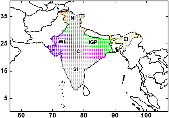
A map of India divided into six regions based on meteorology and variation of aerosols (adapted from David et al., 2018). Spatial distribution of GEOS‐Chem grid points (0.5° × 0.667° resolution) over the Indian region is shown in different colors for the six regions. The domain of the current study is shown by the box. CI = Central India; EI = Eastern India; GEOS = Goddard Earth Observing System; IGP = Indo Gangetic Plain; NI = Northern India; SI = Southern India; WI = Western India.
Table 1 shows the population count along with the anthropogenic PM (black carbon [BC] and organic carbon [OC]) and precursor (SO2, NO, VOCs, and NH3) emission rates (kg/year) over the six regions in India. The details on the emission inventories used in the study are discussed in section 2.2. IGP has the highest population (~2–12 times higher than other regions defined in Figure 1) and emission rates in India, and has a tendency to retain pollution within the region during winter (Kar et al., 2010). SI is second to IGP in population and is roughly ~2 times that of CI; however, emission rates in SI and CI are comparable. NI is the least populated region in India and also has the lowest emission rates.
Table 1.
The Population Count Along With Anthropogenic PM (BC and OC) and Precursor (SO2, NO, VOCs, and NH3) Emission Rate in the Six Regions in India
| Region | Anthropogenic emissions (kg/year) | ||||||
|---|---|---|---|---|---|---|---|
| Population count (×107) | BC (×105) | OC (×105) | NO (×106) | SO2 (×106) | NH3 (×106) | VOCs (×106) | |
| NI | 4.98 | 1.24 | 0.655 | 1.83 | 2.82 | 3.65 | 1.62 |
| IGP | 60.2 | 7.67 | 4.53 | 10.2 | 21.5 | 20.7 | 8.83 |
| EI | 8.51 | 2.17 | 0.903 | 3.33 | 1.46 | 7.20 | 2.99 |
| WI | 14.3 | 3.60 | 2.39 | 4.10 | 10.6 | 7.33 | 4.50 |
| CI | 17.9 | 3.58 | 3.11 | 6.02 | 20.8 | 9.78 | 4.67 |
| SI | 32.5 | 3.93 | 2.92 | 8.79 | 16.4 | 10.6 | 5.79 |
Note. CI = Central India; EI = Eastern India; IGP = Indo Gangetic Plain; NI = Northern India; PM = particulate matter; SI = Southern India; WI = Western India.
2.2. Model Details and Simulation Setup
We used the Goddard Earth Observing System (GEOS)‐Chem global 3‐D chemical‐transport model (v10‐01; Bey et al., 2001) driven with assimilated meteorological data from the GEOS at the NASA Global Modeling and Assimilation Office. GEOS‐Chem includes a detailed simulation of oxidant‐aerosol chemistry with 93 tracers and includes secondary inorganic aerosols (sulfate, nitrate, and ammonium), primary BC and OC, secondary organic aerosols (SOA), sea salt, and dust. We ran global GEOS‐Chem simulations at 2° × 2.5° resolution using GEOS‐5 meteorology to generate temporally varying boundary conditions of all species for higher‐resolution nested simulations at 0.5° × 0.667° resolution over India (~0–41°N latitude, ~56–107°E longitude). The model was spun up for 3 months for initialization. Anthropogenic (BC, OC, and SO2) emissions (monthly) in India were from SMOG (Speciated Multi‐pOllutant Generator from the Indian Institute of Technology (IIT) Bombay; Pandey et al., 2014; Sadavarte & Venkataraman, 2014), and other emissions are described in detail in the supporting information (section S1). In a separate study, David et al. (2018) compared BC, OC, and SO2 emissions from SMOG inventory with BC and OC from Bond et al. (2007) and SO2 from MIX emission inventories. BC and OC emissions in SMOG are higher by a factor of ~5 and 3, respectively, compared to Bond et al. (2007), and SO2 emission is 1.5 times larger than in the MIX inventory. A detailed comparison of SMOG emissions with other inventories over the Indian region is given in Sadavarte and Venkataraman (2014) and Pandey et al. (2014). Simulated PM2.5 was calculated at 35% relative humidity following recommendations in GEOS‐Chem using the following equation:
where NH4, NIT, and SO4 are ammonium, nitrate, and sulfate, respectively; BCPI and OCPI are the hydrophilic BC and OC aerosols, respectively; BCPO and OCPO are the hydrophobic BC and OC aerosols, respectively; SALA is the accumulation mode sea salt aerosol; and DST is the size bins for dust aerosols with effective radii ranging from 0.1 to 1.8 μm. GEOS‐Chem simulations were made for the year 2012. (More details are given in the following URL: http://wiki.seas.harvard.edu/geos-chem/index.php/Particulate_matter_in_GEOS-Chem.)
We performed nine simulations shown in Table 2. The first simulation (S0) is the base simulation with all emissions turned on. Six simulations had anthropogenic PM (BC and OC) and precursor (SO2, NO, VOCs, and NH3) emissions turned off in each of six regions individually (S1–S6 for NI, IGP, EI, WI, CI, and SI, respectively). Comparison of S1–S6 with S0 allows us to determine the impact of anthropogenic emissions from a given region within India on PM2.5 and mortality in other regions. We simulated the model with anthropogenic PM and precursors emissions in India and natural sources in the nested domain turned off to calculate the impact of anthropogenic pollutants transported from regions OI on the six regions (S7). Finally, we performed a simulation where anthropogenic PM and precursor emissions in India were turned off (S8). The difference of simulations S8 and S7 gives the contribution from natural sources (dust, lightning NOx, soil NOx, biogenic VOCs, wildfires, and NH3).
Table 2.
Description of Nine Simulations Performed in GEOS‐Chem
| Simulation No. | Simulation details | |
|---|---|---|
| S0 | All emissions on | Standard simulation |
| S1 | Anthropogenic PM and precursor emissions turned off in Northern India | Sensitivity simulations |
| S2 | Anthropogenic PM and precursor emissions turned off in Indo Gangetic Plain | |
| S3 | Anthropogenic PM and precursor emissions turned off in Eastern India | |
| S4 | Anthropogenic PM and precursor emissions turned off in Western India | |
| S5 | Anthropogenic PM and precursor emissions turned off in Central India | |
| S6 | Anthropogenic PM and precursor emissions turned off in Southern India | |
| S7 | Anthropogenic PM and precursor emissions in India and natural sources in the nested domain turned off | |
| S8 | Anthropogenic PM and precursor emissions in India turned off |
Note. GEOS = Goddard Earth Observing System; PM = particulate matter.
2.3. Estimation of PM2.5‐Related Premature Deaths
We use the baseline mortality rates compiled for Global Burden of Disease 2012 for Ischemic Heart Disease (IHD), CerebroVascular Disease (CeVD), Chronic Obstructive Pulmonary Disease (COPD), and Lung cancer (LC) in India for all ages (Global Burden of Disease, 2015). The baseline mortality rates are reported at the country level. Concentration‐response functions (CRFs) relate exposure to ambient PM2.5 to increased risk of premature mortality from specific diseases. The relative risk (RR) from all PM2.5 sources was calculated using the CRF of Burnett et al. (2014):
Monte‐Carlo simulations were conducted by Burnett et al. (2014) to derive 1,000 sets of coefficients (α, γ, δ, and X0) for each cause (and each age group for CeVD and IHD; the coefficients are available at http://ghdx.healthdata.org/sites/default/files/record-attached-files/IHME_CRCurve_parameters.csv). We use these sets of coefficients to determine the mean (RR total), 5th, and 95th percentiles of mortality. Burnett et al. (2014) assume that (i) the toxicity of PM2.5 is not dependent on composition, (ii) relationship between RR of mortality and PM2.5 exposure is nonlinear, (iii) the RR of mortality is a function of long‐term exposure (e.g., annual‐average PM2.5 concentrations), (iv) CRFs may be applied globally even when the underlying epidemiological studies were done in limited regions, and (v) there exists a minimum PM2.5 threshold (modeled as a uniform distribution ranging between 5.8 and 8.8 μgm−3) below which no further negative health impacts are assumed to occur. Here we consider only uncertainty from the CRF; however, there are other sources (e.g., solid fuel use, baseline mortality rate, and resolution) of uncertainties in these estimates (Kodros et al., 2016, 2018). It is important to note that the concentrations do not linearly translate to RR since the response is roughly logarithmic to aerosol concentration. Chowdhury and Dey (2016) used varying baseline mortality at the state level using the gross domestic product as a proxy and estimated ~15% more premature mortality due to exposure to ambient PM2.5 as opposed to uniform country‐level baseline mortality rate. Kodros et al. (2016) have discussed the increase in mortalities with finer model resolutions. Philip et al. (2017) have estimated that inclusion of anthropogenic fugitive, combustion, and industrial dust emissions in GEOS‐Chem reduced the model bias in PM2.5 from 17% to 7% over East and South Asia in comparison with Surface PM Network measurements. These studies provide an idea of the uncertainties involved in calculating PM2.5 abundances and how they translate to the uncertainties in the calculated RR.
The number of mortalities within model grid cell (0.5° × 0.667°), for each cause of death from PM2.5, is calculated using the following equation:
where y 0 is the age‐specific baseline mortality rate for the respective disease given in Table S1 and POP is the total population. We used 2015 gridded population data from the NASA Socioeconomic Data and Application Center (http://sedac.ciesin.columbia.edu/), which was based on the 2011 India census.
The contribution to mortality in a given region by other regions was calculated by scaling the total mortality of the given region from all PM2.5 by the fraction of PM2.5 coming from each of the other regions (Conibear et al., 2018a; Kodros et al., 2016).
3. Results and Discussions
3.1. Variation in PM2.5 Over India
The simulated annual‐mean surface PM2.5 over India is shown in Figure S1. We had evaluated simulated fine mode Aerosol Optical Depth (AOD) at 500 nm with Aerosol Robotic Network observations over India (David et al., 2018). The simulated fine mode AOD was higher compared to the observations with a slope, correlation coefficient, and mean bias of 1.1 ± 0.02, 0.86, and 0.16 ± 0.26, respectively (David et al., 2018). In this study, our simulated PM2.5 concentrations varied substantially over India, and they were above 90 μg/m3 in IGP and 40–60 μg/m3 over most of the other Indian regions. The lowest values (<10 μg/m3) were observed in portions of NI. The model simulations showed that 99.9% of the Indian population was exposed to annual‐mean PM2.5 concentrations that exceeded the WHO air quality guideline (Conibear et al., 2018a; Venkataraman et al., 2018). The population‐weighted PM2.5 concentration was 75.5 μg/m3. (The population‐weighted PM2.5 is calculated as where PM2.5i and POPi denote the PM2.5 concentration and population in the ith grid, respectively.) The population‐weighted mean PM2.5 concentration was comparable to those noted by Venkataraman et al. (2018) and Cohen et al. (2017). However, the mean values were higher by factors of 1.2–1.3 compared to previous studies for 2011 (Ghude et al., 2016) and 2014 (Conibear et al., 2018a) over India. Figure 2a shows the variation in population‐weighted PM2.5 as calculated from the model along with the total population in the six regions. IGP had the highest population‐weighted PM2.5 compared to other regions (~2 times higher than the next highest region). WI and SI had the lowest PM2.5, followed by CI, EI, and NI. Although the lowest PM2.5 concentration values were found in NI, population‐weighted mean PM2.5 over NI was higher because the part of NI that borders IGP had higher concentrations (Figure S1) of PM2.5. Studies have shown that the residential biomass burning (24%; Venkataraman et al., 2018) or residential energy use (67%; Conibear et al., 2018a) is the large contributor to PM2.5 over most parts of India. The contribution from different sources, agricultural, power, industrial, residential, and transport to population‐weighted PM2.5, was determined for the six regions and shown in Figure S2. The simulation details are also given in section S2. It is observed from Figure S2 that even though contribution from residential sector was the highest (as found in other studies); PM2.5 concentrations were not proportional to total population in each region (Figure 2a). The difference can largely be attributed to import of PM2.5 to a given region.
Figure 2.
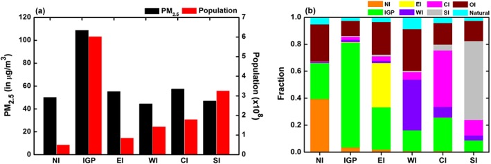
(a) Population‐weighted PM2.5 concentrations along with total population in the region and (b) fraction of PM2.5 or mortality attributed to anthropogenic emissions in each of the six regions from sources (1) within each of the six Indian regions, (2) outside of India, and (3) from natural sources. CI = Central India; EI = Eastern India; IGP = Indo Gangetic Plain; NI = Northern India; OI = outside India; PM = particulate matter; SI = Southern India; WI = Western India.
To investigate the contribution of transport of PM2.5 into a region, we turned off anthropogenic PM and precursor emissions from each region one at a time as described in section 2.2 (Table 2). The reduction in annual‐mean population‐weighted PM2.5 concentration over India with anthropogenic PM and precursor emissions turned off individually from the six regions is shown in Table 3. The population‐weighted PM2.5 concentration was reduced by ~84% by turning off the anthropogenic emissions over all of India. The largest reduction over India was achieved through removal of anthropogenic emissions from IGP (56%), followed by SI (10%) and CI (8%). The smallest regional impact was from emissions in EI (2%). On turning off anthropogenic emissions from OI (S7) and natural sources from the study domain, PM2.5 over India was reduced by ~15% and ~4%, respectively. Since contribution from natural sources is only about 4%, we did not analyze its origins.
Table 3.
The Reduction in Annual‐Mean Population‐Weighted PM2.5 Concentration Over India Caused by Removing Anthropogenic Emissions Individually From the Six Regions
| Region off | PM2.5 (μg/m3) | Percent reduction |
|---|---|---|
| NI | 2.63 | 3 |
| IGP | 42.3 | 56 |
| EI | 1.38 | 2 |
| WI | 3.67 | 5 |
| CI | 6.06 | 8 |
| SI | 7.36 | 10 |
Note. CI = Central India; EI = Eastern India; IGP = Indo Gangetic Plain; NI = Northern India; PM = particulate matter; SI = Southern India; WI = Western India.
Figure 2b shows the fraction of PM2.5 attributed to anthropogenic emissions in each of the six regions from sources (1) within each of the six Indian regions, (2) outside of India, and (3) from natural sources. In all the regions except EI, the anthropogenic emissions from within the region were the largest contributor (38–78%) to population‐weighted PM2.5 concentration. In IGP and SI, anthropogenic emissions from within each region were the largest sources of PM2.5 concentrations, contributing 58–78% of total population‐weighted PM2.5 in that region. In the remaining regions, anthropogenic emissions from within the region contributed less than ~40%, between 3% and 9% came from natural sources, and the rest was transported into these regions.
The transport of PM2.5 from regions OI on population‐weighted PM2.5 concentration was 11% to 31%, and this OI influence was largest for NI, EI, and WI (24–31%). The regions that were most influenced by transport of PM2.5 from other regions within India were EI and CI, with ~40% of the PM2.5 in those regions having been imported, followed by NI, WI, and SI with around 25%. The region least impacted by transport from a region within India was IGP with only about 9% coming from elsewhere. IGP had the largest impact on other regions; it ranged from 8% on SI to 31% on EI (as seen in Figure 2b). CI also transported PM2.5 into WI (6%) and SI (12%), and CI was influenced by WI (8%). The anthropogenic emissions from NI, EI, and SI did not significantly influence PM2.5 in other regions within India. NI, EI, WI, and CI are the regions that were fractionally more impacted (~54–64%) by transport from outside of these individual regions. IGP followed by OI emissions had the most influence on PM2.5 in other regions due to transport. This transport will have a significant influence on how regions plan on dealing with national ambient air quality standards, and it is also a transnational issue due to the large influence of OI on many Indian regions. IGP is the most polluted region due to its own sources, and therefore, it is not influenced significantly by transport of pollutants from other regions; hence, IGP has to reduce its own emissions to improve air quality in that region. Such reductions within IGP will not only help that region, but also its neighbors. Regions such as NI, EI, WI, and CI, with a large fraction of their PM2.5 imported into their region, may not be able to sufficiently control their own PM2.5 levels.
3.2. Mortality Attributed to Ambient PM2.5
We estimated the total premature mortality attributed to exposure to ambient PM2.5 in India as 1.1 (5–95 percentiles: 0.65–1.5) million premature deaths for 2012 in agreement with Cohen et al. (2017). These numbers are likely larger now since emissions have increased during the last 5 years (Rafaj & Amann, 2018). Figure 3a and Table 4 show the mortality for each cause of death due to exposure to ambient PM2.5 over the six regions in India. Figures 2a and 3a, respectively, show that atmospheric PM2.5 pollution and related premature mortality vary substantially across the six regions. The IGP, due to its large population, and export of PM to other regions account for close to 50% of the premature mortality associated with ambient PM2.5 exposure over all of India, followed by SI (21%) and CI (12%). The remaining regions (NI, EI, and WI) each individually contribute <10% of the PM2.5‐attributed mortalities (17% total across the three regions) over India. The disease burden attributed to exposure to ambient PM2.5 is dominated by IHD (~44%) and CeVD (~33%) over India; similar results with lower mortality estimates were reported by Ghude et al. (2016). From discussions in section 3.1, it is evident that atmospheric transport impacts PM2.5 concentrations in each of the six regions, and the mortality associated with transport of PM2.5 is discussed in the following section. Figure 3b shows the annual mortality attributed to PM2.5 per million people in the six regions. Higher PM2.5 concentrations along with high population in the IGP lead to greater (>900) premature mortality per million people. In the other regions, the premature mortality per million people was slightly smaller but comparable (~680–750). It is important to note that lower total numbers were due mainly to the lower populations.
Figure 3.
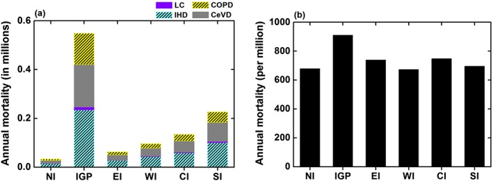
Total annual premature deaths attributed to PM2.5 (a) by cause of death and (b) per million people over the six regions in India. CeVD = cerebrovascular disease; CI = Central India; COPD = chronic obstructive pulmonary disease; EI = Eastern India; IGP = Indo Gangetic Plain; IHD = ischemic heart disease; LC = lung cancer; NI = Northern India; PM = particulate matter; SI = Southern India; WI = Western India.
Table 4.
The Annual Mortalities (in Hundreds) by Cause of Death in the Six Regions in India Attributed to Exposure to PM2.5
| Regions | IHD | LC | CeVD | COPD | Total |
|---|---|---|---|---|---|
| NI | 151 (110–217) | 6 (3–8) | 113 (46–145) | 66 (37–93) | 336 (196–463) |
| IGP | 2343 (1696–3450) | 122 (78–152) | 1741 (765–2055) | 1278 (812–1652) | 5484 (3351–7309) |
| EI | 277 (200–404) | 12 (6–16) | 216 (84–272) | 125 (70–174) | 630 (360–866) |
| WI | 429 (313–615) | 17 (9–24) | 332 (129–430) | 182 (99–260) | 960 (550–1329) |
| CI | 588 (425–862) | 26 (14–34) | 463 (180–581) | 268 (152–372) | 1345 (771–1849) |
| SI | 1007 (732–1452) | 41 (21–57) | 784 (304–1009) | 434 (237–616) | 2266 (1294–3134) |
Note. CeVD = cerebrovascular disease; CI = Central India; EI = Eastern India; COPD = chronic obstructive pulmonary disease; IGP = Indo Gangetic Plain; IHD = ischemic heart disease; LC = lung cancer; NI = Northern India; PM = particulate matter; SI = Southern India; WI = Western India. The numbers in parentheses is the 5th and 95th percentiles calculated from uncertainties in the concentration‐response function.
3.2.1. Effects of Atmospheric Transport of PM2.5 on Regional Mortality
Regional atmospheric pollution and related health impacts can be attributed to emissions from both local and other regions as a result of atmospheric transport. Figure 2b accounts for premature mortality as well as PM2.5 since it is a proportional relationship. We find that ~24–32% of premature mortality in NI, EI, and WI and ~12–16% in IGP, CI, and SI was caused by PM2.5 transported from OI. The mortality due to PM2.5 transported from different regions within India ranged from ~9–39%, with the highest transport into EI (39%), followed by CI (37%). The natural sources contributed ~3–9% mortality within India; the highest impact of natural sources was in WI (9%). Figure 4 shows the effect of atmospheric transport on premature mortality in the six regions due to PM2.5 (anthropogenic) produced in other regions and natural sources. The inset in Figure 4 shows the contribution of anthropogenic emissions in the different regions to total mortality in India. More than 50% of the premature deaths in NI, EI, WI, and CI were due to transport of PM2.5 from regions outside of these individual regions (Figures 2b and 4). Figure 5 shows the influence of IGP emissions on the population within IGP as well as in other regions. Transport of PM2.5 from IGP resulted in 24–31% mortality in NI, EI, and CI; highest impact was in EI (31%). IGP has minimal influence (~8%) on SI. Close to 20% of the impact of IGP emissions is outside of this region. In addition to IGP, CI also influences outside of the region. CI emissions contributed to 12% and 6%, respectively, in SI and WI. The mortality due to transport of PM2.5 from NI, EI, and SI was <5% in other regions. The region least impacted by transport of PM2.5 was IGP; about 76% of mortality in IGP was caused by emissions within that region. Similarly, ~58% of premature mortality in SI was due to emissions from this region.
Figure 4.
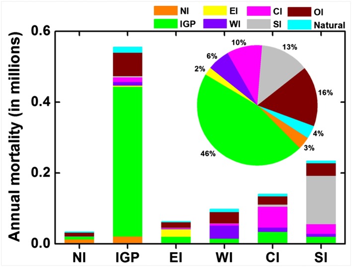
Regional premature mortality attributed to regions where anthropogenic emissions were produced along with contributions from natural sources in the six regions. The inset shows the contribution of anthropogenic emissions in the individual six regions as well as transport from outside India and natural emissions to total mortality in India. CI = Central India; EI = Eastern India; IGP = Indo Gangetic Plain; NI = Northern India; OI = outside India; SI = Southern India; WI = Western India.
Figure 5.
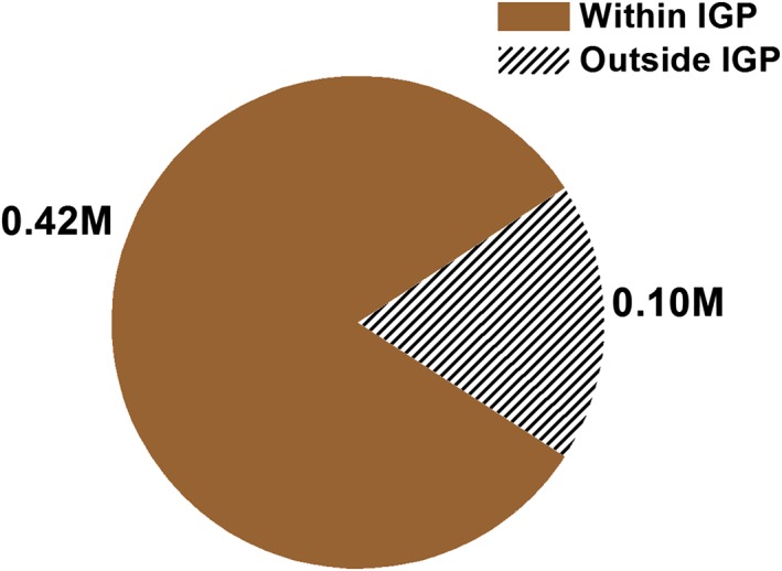
Pie chart shows the mortality, in millions, (a) within IGP (brown) and (b) outside IGP (hatched) in India due to anthropogenic emissions in IGP. Clearly, 20% of the premature mortality due to IGP emissions is outside of IGP. IGP = Indo Gangetic Plain.
In this study, we estimated the total premature mortality due to PM2.5 as 1.1 million; 16% of the total premature deaths in India were caused by anthropogenic pollutants transported from OI and ~4% due to natural sources. About 80% of the total premature mortality was caused by anthropogenic emissions from India; the contribution from anthropogenic emissions in IGP (~46%) was highest, followed by SI (~13%). The transport of pollutants between different regions within India caused ~19% of the total premature mortality; of this, transport of anthropogenic emissions from IGP and CI contributed, respectively, 8% and 4%, with the remaining from other regions. In contrast, Zhao et al. (2017) have shown that the total premature deaths caused by pollution transported from regions outside China were less than 1%. Clearly, reduction in anthropogenic emissions over India, as in the case of China, will be able to reduce the health burden substantially. However, unlike China, transport from outside the country is also an important contributor for India.
The estimated premature mortality due to exposure to PM2.5 was compared with previous studies over India and shown in Figure S3. The estimated total premature mortality in this study was within 1% compared to Cohen et al. (2017), which had similar annual PM2.5 concentrations as mentioned in section 3.1. It was within 20% of that reported by Conibear et al. (2018a) (11%), and Lelieveld (2017) (19%), but higher by a factor of ~2–3 compared to other studies. It should be noted that the studies for estimation of premature mortality in India vary with model resolution, population year, baseline mortality rate, CRF, and PM2.5 concentrations (emission inventories), all of which may lead to different total premature mortality estimates. However, we expect that the relative contributions due to transport is much less variant than the total estimated mortality. We note that other studies generally did not explore transport from outside the region.
Conibear et al. (2018b) showed that stringent emission control policies in India can reduce the increasing health impacts from air pollution. Liang et al. (2018) studied the impact of intercontinental transport of PM2.5 on mortality in South Asia by reducing the emissions in different regions by 20%. Their study showed that South Asia is most impacted by PM2.5 emissions from the Middle East. Our study shows that reduction in anthropogenic emissions in IGP and CI will not only reduce their own mortality but also reduce premature mortality in other regions, especially NI, EI, and CI (impact from IGP) and SI (impact from CI).
Our study emphasizes that finer spatial resolution studies within IGP and CI are needed to understand the current sources (stationary and sector specific) of pollution and their impacts on ambient PM2.5, both from primary PM and precursors. It is also important to note that the consequences of high PM2.5 concentrations in India is not limited to urban regions and extends to rural areas. The majority of premature mortality due to PM2.5 is in rural rather than urban regions (Karambelas et al., 2018). Our study, along with the previous ones, clearly show the need for large‐scale regional monitoring in addition to those sparse measurements in urban areas. Lastly, we note that the aerosol loading in a given region is mostly dependent on the emission inventories and meteorology that transport aerosols and aerosol precursors. However, the fractional contributions from the different regions are mostly dependent on transport, which are relatively well defined. Therefore, the smaller uncertainties in transport would not greatly influence the calculated total burden of mortality.
Conflict of Interest
The authors declare no conflicts of interest relevant to this study.
Supporting information
Supporting Information S1
Table S1
Acknowledgments
The work was funded by Colorado State University. The model data used in this study are available at http://biodav.atmos.colostate.edu/ldavid/GC_PM25_2012/. Special thanks to Matthew Bishop for downloading the GEOS‐5 meteorological files. India nested version of GEOS‐Chem was developed by Sreelekha Chaliyakunnel and Dylan B Millet (University of Minnesota). GEOS‐5 meteorology at 0.5° × 0.667° resolution over India was provided by Chi Li (Dalhousie University).
David, L. M. , Ravishankara, A. R. , Kodros, J. K. , Pierce, J. R. , Venkataraman, C. , & Sadavarte, P. (2019). Premature mortality due to PM2.5 over India: Effect of atmospheric transport and anthropogenic emissions. GeoHealth, 3, 2–10. 10.1029/2018GH000169
This article was corrected on 15 JUL 2019. The online version of this article has been modified to include a Conflict of Interest statement.
Contributor Information
Liji M. David, Email: lijimdavid@gmail.com.
A. R. Ravishankara, Email: a.r.ravishankara@colostate.edu.
References
- Amann, M. , Purohit, P. , Bhanarkar, A. D. , Bertok, I. , Borken‐Kleefeld, J. , Cofala, J. , Heyes, C. , Kiesewetter, G. , Klimont, Z. , Liu, J. , Majumdar, D. , Nguyen, B. , Rafaj, P. , Rao, P. S. , Sander, R. , Schöpp, W. , Srivastava, A. , & Vardhan, B. H. (2017). Managing future air quality in megacities: A case study for Delhi. Atmospheric Environment, 161, 99–111. 10.1016/j.atmosenv.2017.04.041 [DOI] [Google Scholar]
- Bey, I. , Jacob, D. J. , Yantosca, R. M. , Logan, J. A. , Field, B. D. , Fiore, A. M. , Li, Q. , Liu, H. Y. , Mickley, L. J. , & Schultz, M. G. (2001). Global modeling of tropospheric chemistry with assimilated meteorology: Model description and evaluation. Journal of Geophysical Research, 106(D19), 23,073–23,095. 10.1029/2001JD000807 [DOI] [Google Scholar]
- Bond, T. C. , Bhardwaj, E. , Dong, R. , Jogani, R. , Jung, S. , Roden, C. , Streets, D. G. , & Trautmann, N. M. (2007). Historical emissions of black and organic carbon aerosol from energy‐related combustion, 1850‐2000. Global Biogeochemical Cycles, 21, GB2018 10.1029/2006GB002840 [DOI] [Google Scholar]
- Brown, J. , Gordon, T. , Price, O. , & Asgharian, B. (2013). Thoracic and respirable particle deinitions for human health risk assessment. Particle and Fibre Toxicology, 10(1), 12 10.1186/1743-8977-10-12 [DOI] [PMC free article] [PubMed] [Google Scholar]
- Burnett, R. T. , Arden Pope, C. , Ezzati, M. , Olives, C. , Lim, S. S. , Mehta, S. , et al. (2014). An integrated risk function for estimating the global burden of disease attributable to ambient fine particulate matter exposure. Environmental Health Perspectives, 122(4), 397–403. 10.1289/ehp.1307049 [DOI] [PMC free article] [PubMed] [Google Scholar]
- Chowdhury, S. , & Dey, S. (2016). Cause‐specific premature death from ambient PM2.5exposure in India: Estimate adjusted for baseline mortality. Environment International, 91, 283–290. 10.1016/j.envint.2016.03.004 [DOI] [PubMed] [Google Scholar]
- Cohen, A. J. , Brauer, M. , Burnett, R. , Anderson, H. R. , Frostad, J. , Estep, K. , Balakrishnan, K. , Brunekreef, B. , Dandona, L. , Dandona, R. , Feigin, V. , Freedman, G. , Hubbell, B. , Jobling, A. , Kan, H. , Knibbs, L. , Liu, Y. , Martin, R. , Morawska, L. , Pope, C. A. , Shin, H. , Straif, K. , Shaddick, G. , Thomas, M. , van Dingenen, R. , van Donkelaar, A. , Vos, T. , Murray, C. J. L. , & Forouzanfar, M. H. (2017). Estimates and 25‐year trends of the global burden of disease attributable to ambient air pollution: An analysis of data from the Global Burden of Diseases Study 2015. The Lancet, 389(10082), 1907–1918. 10.1016/S0140-6736(17)30505-6 [DOI] [PMC free article] [PubMed] [Google Scholar]
- Conibear, L. , Butt, E. W. , Knote, C. , Arnold, S. R. , & Spracklen, D. V. (2018a). Residential energy use emissions dominate health impacts from exposure to ambient particulate matter in India. Nature Communications, 9(1), 617–619. 10.1038/s41467-018-02986-7 [DOI] [PMC free article] [PubMed] [Google Scholar]
- Conibear, L. , Butt, E. W. , Knote, C. , Arnold, S. R. , & Spracklen, D. V. (2018b). Stringent emission control policies can provide large improvements in air quality and public health in India. GeoHealth, 2, 196–211. 10.1029/2018GH000139 [DOI] [PMC free article] [PubMed] [Google Scholar]
- David, L. M. , Ravishankara, A. R. , Kodros, J. K. , Venkataraman, C. , Sadavarte, P. , Pierce, J. R. , Chaliyakunnel, S. , & Millet, D. B. (2018). Aerosol optical depth over India. Journal of Geophysical Research: Atmospheres, 123, 3688–3703. 10.1002/2017JD027719 [DOI] [PMC free article] [PubMed] [Google Scholar]
- Ghosh, S. , Biswas, J. , Guttikunda, S. , & Roychowdhury, S. (2015). An investigation of potential regional and local source regions affecting fine particulate matter concentrations in Delhi, India. Journal of the Air & Waste Management Association, 65(2), 218–231. 10.1080/10962247.2014.982772 [DOI] [PubMed] [Google Scholar]
- Ghude, S. , Chate, D. M. , Jena, C. , Beig, G. , Kumar, R. , Barth, M. C. , Pfister, G. G. , Fadnavis, S. , & Pithani, P. (2016). Premature mortality in India due to PM2.5 and ozone exposure. Geophysical Research Letters, 43, 4650–4658. 10.1002/2016GL068949 [DOI] [Google Scholar]
- Global Burden of Disease Study 2015 (2015). Results (p. 2016). Seattle, United States: Institute for Health Metrics and Evaluation (IHME). [Google Scholar]
- India Office of the Registrar General and Census Commissioner (2011). Census of India. New Delhi: Ministry of Home Affairs, Government of India. [Google Scholar]
- Kar, J. , Deeter, M. N. , Fishman, J. , Liu, Z. , Omar, A. , Creilson, J. K. , Trepte, C. R. , Vaughan, M. A. , & Winker, D. M. (2010). Wintertime pollution over the Eastern Indo‐Gangetic Plains as observed from MOPITT, CALIPSO and tropospheric ozone residual data. Atmospheric Chemistry and Physics, 10(24), 12,273–12,283. 10.5194/acp-10-12273-2010 [DOI] [Google Scholar]
- Karambelas, A. , Holloway, T. , Kinney, P. L. , Fiore, A. M. , De Fries, R. , Kiesewetter, G. , & Heyes, C. (2018). Urban versus rural health impacts attributable to PM2.5 and O3 in northern India. Environmental Research Letters, 13(6). 10.1088/1748-9326/aac24d [DOI] [Google Scholar]
- Kodros, J. K. , Carter, E. , Brauer, M. , Volckens, J. , Bilsback, K. R. , L'Orange, C. , Johnson, M. , & Pierce, J. R. (2018). Quantifying the contribution to uncertainty in mortality attributed to household, ambient, and joint exposure to PM 2.5 from residential solid fuel use. GeoHealth, 2, 25–39. 10.1002/2017GH000115 [DOI] [PMC free article] [PubMed] [Google Scholar]
- Kodros, J. K. , Wiedinmyer, C. , Ford, B. , Cucinotta, R. , Gan, R. , Magzamen, S. , & Pierce, J. R. (2016). Global burden of mortalities due to chronic exposure to ambient PM2.5 from open combustion of domestic waste. Environmental Research Letters, 11(12), 1–9. 10.1088/1748-9326/11/12/124022 [DOI] [Google Scholar]
- Lee, B. K. , & Hieu, N. T. (2011). Seasonal variation and sources of heavy metals in atmospheric aerosols in a residential area of Ulsan, Korea. Aerosol and Air Quality Research, 11(6), 679–688. 10.4209/aaqr.2010.10.0089 [DOI] [Google Scholar]
- Lelieveld, J. (2017). Clean air in the Anthropocene. Faraday Discussions, 200, 693–703. 10.1039/c7fd90032e [DOI] [PubMed] [Google Scholar]
- Lelieveld, J. , Barlas, C. , Giannadaki, D. , & Pozzer, A. (2013). Model calculated global, regional and megacity premature mortality due to air pollution. Atmospheric Chemistry and Physics, 13(14), 7023–7037. 10.5194/acp-13-7023-2013 [DOI] [Google Scholar]
- Lelieveld, J. , Evans, J. S. , Fnais, M. , Giannadaki, D. , & Pozzer, A. (2015). The contribution of outdoor air pollution sources to premature mortality on a global scale. Nature, 525(7569), 367–371. 10.1038/nature15371 [DOI] [PubMed] [Google Scholar]
- Liang, C.‐K. , Jason West, J. , Silva, R. A. , Bian, H. , Chin, M. , Dentener, J. , Davila, Y. , Emmons, L. , Folberth, G. , Flemming, J. , Henze, D. , Im, U. , Jonson, J. E. , Kucsera, T. , Keating, T. J. , Lund, M. T. , Lenzen, A. , Lin, M. , Pierce, R. B. , Park, R. J. , Pan, X. , Sekiya, T. , Sudo, K. , & Takemura, T. (2018). HTAP2 multi‐model estimates of premature human mortality due to intercontinental transport of air pollution, (January). Atmospheric Chemistry and Physics Discussions. 10.5194/acp-2017-1221 [DOI] [PMC free article] [PubMed] [Google Scholar]
- Liu, J. , Mauzerall, D. L. , & Horowitz, L. W. (2009). Evaluating inter‐continental transport of fine aerosols: (2) Global health impact. Atmospheric Environment, 43(28), 4339–4347. 10.1016/j.atmosenv.2009.05.032 [DOI] [Google Scholar]
- Pandey, A. , Sadavarte, P. , Rao, A. B. , & Venkataraman, C. (2014). A technology‐linked multi‐pollutant inventory of Indian energy‐use emissions: II. Residential, agricultural and informal industry sectors. Atmospheric Environment, 99, 341–352. 10.1016/j.atmosenv.2014.09.080 [DOI] [Google Scholar]
- Philip, S. , Martin, R. V. , Snider, G. , Weagle, C. L. , Van Donkelaar, A. , Brauer, M. , Henze, D. K. , Klimont, Z. , Venkataraman, C. , Guttikunda, S. K. , & Zhang, Q. (2017). Anthropogenic fugitive, combustion and industrial dust is a significant, underrepresented fine particulate matter source in global atmospheric models. Environmental Research Letters, 12(4). 10.1088/1748-9326/aa65a4 [DOI] [Google Scholar]
- Raes, F. , Van Dingenen, R. , Elisabetta, V. , Wilson, J. , Putaud, J. P. , Seinfeld, J. H. , & Adams, P. (2000). Chapter 18 formation and cycling of aerosols in the global troposphere. Developments in Environmental Science, 1(C), 519–563. 10.1016/S1474-8177(02)80021-3 [DOI] [Google Scholar]
- Rafaj, P. , & Amann, M. (2018). Decomposing air pollutant emissions in Asia: Determinants and projections. Energies, 11(5), 1299 10.3390/en11051299 [DOI] [Google Scholar]
- Sadavarte, P. , & Venkataraman, C. (2014). Trends in multi‐pollutant emissions from a technology‐linked inventory for India: I. industry and transport sectors. Atmospheric Environment, 99, 353–364. 10.1016/j.atmosenv.2014.09.081 [DOI] [Google Scholar]
- Venkataraman, C. , Brauer, M. , Tibrewal, K. , Sadavarte, P. , Ma, Q. , & Cohen, A. (2018). Source influence on emission pathways and ambient PM2.5 pollution over India (2015–2050). Atmospheric Chemistry and Physics, 18, 8017–8039. [DOI] [PMC free article] [PubMed] [Google Scholar]
- World Health Organization . (2016). Ambient air pollution: A global assessment of exposure and burden of disease. World Health Organization. Retrieved from http://www.who.int/iris/handle/10665/25014
- Zhao, H. , Li, X. , Zhang, Q. , Jiang, X. , Lin, J. , Peters, G. P. , Li, M. , Geng, G. , Zheng, B. , Huo, H. , Zhang, L. , Wang, H. , Davis, S. J. , & He, K. (2017). Effects of atmospheric transport and trade on air pollution mortality in China. Atmospheric Chemistry and Physics, 17(17), 10,367–10,381. 10.5194/acp-17-10367-2017 [DOI] [Google Scholar]
Associated Data
This section collects any data citations, data availability statements, or supplementary materials included in this article.
Supplementary Materials
Supporting Information S1
Table S1