Long-term stability of cortical population dynamics underlying consistent behavior

Abstract

Animals readily execute learned behaviors in a consistent manner over long periods of time, yet no equally stable neural correlate has been demonstrated. How does the cortex achieve this stable control? Using the sensorimotor system as a model of cortical processing, we investigated the hypothesis that the dynamics of neural latent activity, which capture the dominant co-variation patterns within the neural population, must be preserved across time. We recorded from populations of neurons in premotor, primary motor, and somatosensory cortices as monkeys performed a reaching task, for up to two years. Intriguingly, despite steady turnover in the recorded neurons, the low-dimensional latent dynamics remained stable. The stability allowed reliable decoding of behavioral features for the entire timespan, while fixed decoders based directly on the recorded neural activity degraded substantially. We posit that stable latent cortical dynamics within the manifold are the fundamental building blocks underlying consistent behavioral execution.

INTRODUCTION

To reliably execute learned actions, the cortex must integrate sensory information, establish a motor plan, and generate appropriate commands to muscles. Animals, including humans, readily perform such behaviors with remarkable consistency, even years after acquiring the skill. How does the brain achieve this stability? Is the process of integration and planning as stable as the behavior itself? Here, we explore these fundamental questions from the perspective of populations of cortical neurons.

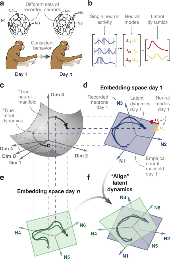
Recent theoretical and experimental work posits that neural function is built on the activation of specific population-wide activity patterns – neural modes – rather than on the independent modulation of individual neurons^1–3. These neural modes are the dominant co-variation patterns within the neural population¹. The set of neural modes defines a neural manifold^1,3,4, a surface that captures much of the variance in the recorded neural activity (Fig. 1). We refer to the time-dependent activation of the neural modes as their latent dynamics^1,5,6. In this framework, the activity of each recorded neuron expresses a weighted combination of the latent dynamics from all the modes^1,7,8 (Fig. 1b). We hypothesized that the latent dynamics underlying consistent behavior must be similarly stable. These latent dynamics exist in a relatively low-dimensional manifold embedded in a high-dimensional neural space whose axes correspond to each of the neurons modulated during the behavior (Fig. 1c). In experimental scenarios, the activity of the full neural population within the cortex can only be partially sampled. However, the neural modes can be empirically estimated from recorded activity by applying dimensionality reduction techniques⁹ such as principal component analysis^1,8 (PCA) to construct an empirical low-dimensional manifold embedded in the empirical neural space spanned by the recorded neurons⁸ (Fig. 1d,e). The latent dynamics within this empirical manifold are an estimate of the true latent dynamics within the full neural space. Quantifying the stability of the latent dynamics is challenging because current recording techniques are unable to sample a stable set of neurons over long periods^10,11.

Figure 1.

Hypothesis. (a) Subjects perform the same behavior over days, yet in typical experimental setups the same neurons cannot be recorded over this period. (b) In our model, the single neuron activity results from a weighted combination of the latent dynamics of the neural modes. (c) The latent dynamics (black line, arrow indicates passage of time) underlying a behavior are mostly confined to a “true” manifold (gray surface) within the full D-dimensional neural space that involves all neurons modulated by the task. (d) The activity of the recorded neurons (N1, N2, N3 in this example) is represented in an empirical neural space in which each axis corresponds to the activity of one recorded neuron. During behavior, the recorded population activity describes a trajectory (blue trace). During movement, such trajectories are typically confined to a low-dimensional neural manifold (blue plane). The projections of the population activity onto the two axes that define the neural manifold in this example are the empirical latent dynamics. (e) Latent dynamics during the same behavior but on a different day, with a different set of recorded neurons. We hypothesize that the true latent dynamics for a given behavior will be stable during repeated execution across days, even when the empirical manifold to which the latent dynamics are confined is embedded in a different empirical neural space. (f) We predict that, in the face of neural turnover, the stable latent dynamics can be recovered by linear alignment.

Here, we developed a method to examine the stability of the underlying latent dynamics despite unavoidable changes in the set of neurons recorded using chronically implanted microelectrode arrays (Fig. 1a). With this method, we assessed the stability of the latent dynamics during consistent behavior, using the sensorimotor system as a model of cortical processing. We recorded the activity of neural populations, approximately one hundred neurons at a time, in each of three different cortical areas – dorsal premotor cortex (PMd), primary motor cortex (M1), and primary somatosensory cortex (S1) – as monkeys performed a center-out reaching behavior. PMd is critical for movement planning, exhibiting strong pre-movement preparatory activity¹² that can be used to predict the intended movement well before it occurs¹³. M1 is the primary cortical area from which descending output to the spinal cord arises¹⁴, and its activity is tightly coupled to the dynamics of motor execution^15,16, even during motor adaptation¹⁷. Lastly, area 2 of S1 integrates somatosensory feedback^18,19, which is essential for the correction of ongoing movements²⁰.

Throughout recordings spanning up to two years, latent dynamics were remarkably stable in all three cortical regions despite turnover of the recorded neurons. Once identified, the stable latent dynamics enabled accurate predictions of various behavioral features using the same “decoder” throughout these long timespans. We found that aligning latent dynamics within the empirical neural manifold (Fig. 1f) was crucial to stabilize the neural activity, and that success could not be attributed to simpler phenomena such as movement information in the activity of individual neurons. Therefore, we identified a neural correlate of stable behavior: the low-dimensional latent dynamics embedded in the full-dimensional cortical neural space. We posit that analogous stable latent dynamics may underlie a variety of learned brain functions, from stimulus recognition to complex cognitive processes.

RESULTS

Hypothesis and approach

We studied the stability of the latent dynamics within the neural manifold and their relationship with consistent behavior (Fig. 1a) over many days. Our theoretical framework posits that the empirical latent dynamics observed on different days (Fig. 1d,e) will differ because they result from projecting the true manifold (Fig. 1c) onto different empirical neural manifolds (after this section, simply “manifolds”) embedded in different empirical neural spaces. It is the stability of the true latent dynamics that we wish to establish. To identify the neural modes that span the manifold, we represented the activity of each recorded neuron along one axis in an embedding neural space^1,3,4,8. In the toy example in Fig. 1d, the number of recorded neurons, and thus the dimensionality d of the neural space, is three. The neural modes can be computed using any dimensionality reduction method that identifies patterns of neural covariation⁹ (here we used PCA; see Methods). Mathematically, the PC axes are the neural modes that span the manifold¹ (blue plane in Fig. 1d).

Changes in the specific neurons recorded over days necessarily cause a change in the axes that define the embedding neural space, along with a corresponding change in the empirically estimated manifold and latent dynamics (Fig. 1d,e). We need to compensate for these changes in order to evaluate the stability of the true latent dynamics governing cortical function (Fig. 1c–e). Note that the projection from the full neural space to the empirical neural space of recorded neurons is a linear transformation, and that PCA identifies a linear empirical neural manifold within the empirical neural space. We conjectured that if the true latent dynamics during repeated task execution were indeed stable, a simple linear transformation should be sufficient to compensate for these changes (Fig. 1f). If, on the contrary, the true latent dynamics were to change fundamentally across days, e.g., due to a change in the intrinsically nonlinear dynamics of the network²¹, no linear transformation would be able to compensate for these changes. We developed a method based on canonical correlation analysis^5,21 (CCA; see Methods) to compensate for changes in recorded neurons and to compare the empirical latent dynamics across days. We describe this process as “aligning” the latent dynamics. In the following sections, we test the hypothesis that stable latent dynamics underlie consistent behavior by analyzing neural population activity recorded in sensorimotor cortex over times spanning weeks to years.

Behavior

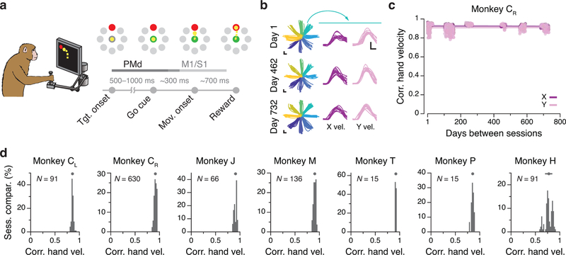
We trained six monkeys (Monkeys C, M, T, J, H, P) to perform a center-out reaching task while using a planar manipulandum (Methods; Fig. 2a). The monkey started each trial by holding at the central target. Then, one of eight outer targets was presented. After a variable delay period, an auditory “go cue” instructed the monkey to move the manipulandum to the intended target, to receive a liquid reward (Fig. 2a). Across monkeys, the time between all recordings spanned from ~20 to ~750 days (see Supplementary Table 1). The behavioral performance of all monkeys was consistent across these time spans, as exemplified by the hand trajectories in Fig. 2b. To quantify stability, we computed the correlation between the X and Y hand velocities across single trials for a given target, for all pairs of days (Fig. 2c). In all of the cases, these correlations were large (mean >0.77, Fig 2d; Extended Data 1).

Figure 2.

Task and repeatability of behavior. (a) Monkeys performed an instructed-delay reaching task using a planar manipulandum. The schematic of the task indicates the approximate time windows used for analysis; these varied across cortical areas (PMd, M1, and S1). (b) Left: Example hand trajectories for three days spanning 731 days from Monkey C_R. Each trace is an individual trial; traces are color-coded based on target location. Right: Example X and Y hand velocity traces for all reaches to the upper-right target on each of the three days. (c) Correlation (Pearson’s r) between direction-matched single trial X and Y hand velocities across all pairs of days from Monkey C_R (single dots: individual pair of days; lines: linear fits). (d) Distribution of across-day hand velocity correlations (Pearson’s r) for all pairs of days for each of the seven sets of implants. Top error bars: mean ± s.d. N: number of across-day comparisons.

Changes in neural recordings across days

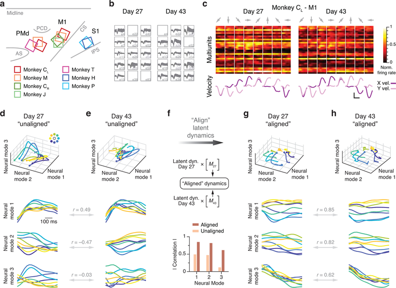
We studied the neural basis for consistent behavior using microelectrode arrays chronically implanted in the arm area of three different regions of cortex in six different monkeys (note that Monkey C received sequential implants in the right and left hemispheres; Methods). Fig. 3a shows the approximate locations of the implanted arrays. Monkeys C_L and M had dual implants in PMd and M1; Monkeys J and C_R had a single implant in M1; Monkey T had an implant in PMd; and Monkeys H and P had an implant in Area 2 of S1. As illustrated by the M1 dataset from of Monkey C_L (Fig. 3b–c), neural activity on each electrode changed dramatically over 15 days (see also Extended Data 2, 3). We assessed the implications of neural turnover by fitting tuning curves relating neural activity to the reach direction (Methods). We found that mean firing rate, modulation depth, and preferred direction changed progressively over time, as shown in Extended Data 4 for all monkeys and all recorded cortical regions. For this and all subsequent analyses, we used the multiunit activity recorded on each electrode, which allowed for an accurate reconstruction of the latent dynamics⁷; our results were similar when using spike-sorted single neurons. Much of this change can be explained by turnover in the specific neurons recorded on each electrode (Extended Data 2, 3). The challenge in testing our hypothesis resides in compensating for these changes in recorded neurons.

Figure 3.

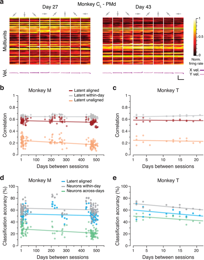
Neural recording and changes in neural activity across days. (a) Approximate location of all nine arrays; each color represents a different set of implants (legend). AS, arcuate sulcus; PCD, precentral dimple; CS, central sulcus; IPS, intraparietal sulcus. (b) Multi-unit threshold crossings for example recording channels on Day 27 and Day 43 for Monkey C_L. (c) Example mean neural firing rates aligned to movement onset for 30 recording channels on the same two days (top; each neuron shown in a different row) and corresponding hand velocity (bottom). The columns represent the average of all trials to each of the eight reach directions (indicated by the arrows above each column). Note the substantial changes in neural activity, reflected in altered firing rates and spatial tuning on each electrode, despite the consistency of the behavior. Scale bars: horizontal, 300 ms; vertical, 10 cm/s. (d-e) Representative Day 27 (d) and Day 43 (e) original (‘unaligned”) M1 latent trajectories for Monkey C_L. Top plots show the latent dynamics in the manifold spanned by the three leading neural modes (dots indicate movement onset), and the lower plots show their projection onto each mode. Data averaged over all trials for each target and aligned to movement onset, only for visualization purposes. Correlation (Pearson’s r) between pairs of corresponding neural modes is indicated. (f) We aligned the trajectories using the CCA matrices M (see Methods). The “aligned” Day 27 (g) and Day 43 (h) latent trajectories show that the magnitude of the correlations were greatly increased by the alignment procedure.

Primary motor cortex during movement control

We now consider whether stable latent dynamics within the cortex underlie the generation of consistent behavior, starting with the analysis of M1 activity during movement execution. We applied our method to align the latent dynamics across days, even as the number and identity of recorded neurons changed. Using single trial neural data, we computed the manifold and the latent dynamics within it using PCA separately for each day (Methods). The dimensionality of the manifold for each brain region (M1: 10; PMd: 15; S1: 8) was selected based on previous studies^5,22. Using CCA^5,21, we found the linear transformations M that made the latent dynamics from subsequent days maximally correlated to those of day one (Methods), to compensate for changes in the empirical embedding space due to turnover in the recorded neurons. As described above, if the true latent dynamics during consistent behavior were indeed stable, the trajectories of the latent dynamics would be very similar after alignment (Fig. 1f): the leading canonical correlations (CCs) would approach a value of one. On the contrary, if true latent dynamics within the brain were unstable for repeated behavior, the trajectories would differ even after attempted alignment, and the resulting CCs would remain low.

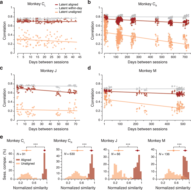
While the trajectories described by the latent dynamics for M1 datasets separated by 16 days were different (Fig. 3c,d), they became quite similar after alignment with CCA (Fig. 3f–g). This observation held for all pairwise combinations of days: the aligned latent dynamics remained stable for the full length of time we recorded from this monkey (red trace in Fig. 4a).

Figure 4.

Stability of M1 latent dynamics over time. (a) Correlation of the aligned (CCs; red) and unaligned (Pearson’s r; orange) M1 latent dynamics averaged over the top four neural modes across all pairs of days from Monkey C_L (single dots: pairs of days; lines: linear fits). The aligned latent dynamics maintained a higher correlation across days than the unaligned dynamics, and were almost as correlated across different days as the latent dynamics across different blocks of trials from the same day (gray). (b)-(d) Same as (a) for the other three M1 implants. (e) Normalized similarity of the aligned and unaligned across-days M1 latent dynamics during movement execution for each monkey (each shown in a different panel). The mean normalized similarity of the aligned latent dynamics across different days is close to 1; this indicates that their canonical correlations are almost as strong as the canonical correlations of the latent dynamics across two blocks of trials from the same day. *** indicates P < 0.001, two-sided Wilcoxon rank-sum test. Error bars: mean ± s.d. N: number of across-day comparisons.

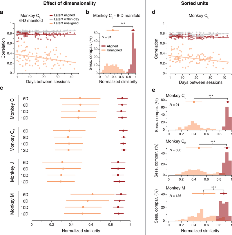
To interpret the magnitude of this across-day stability, we compared it to an upper bound on the achievable CCs, provided by the stability across random blocks of trials within each day (Methods). For this monkey, the across-day CCs were almost identical to the within-day CCs (red and gray traces in Fig. 4a). To summarize these results, we computed a normalized similarity: the ratio of the across-day CCs to the corresponding within-day CCs. For this dataset, the normalized similarity of the latent dynamics after alignment with CCA was 0.93 ± 0.03 (mean ± s.d.; Fig. 4e). The normalized similarity without alignment was much lower (0.38 ± 0.14; Fig. 4e). We obtained similar results for all M1 datasets, comprising four implants from three different monkeys for up to two years (Fig. 4b–e). These results held for a range of manifold dimensionalities from 6 to 12 (Extended Data 5a–c), and also when using sorted neurons to identify the manifold (Extended Data 5d,e). Thus, M1 latent dynamics during repeated movement generation are stable for very long periods of time.

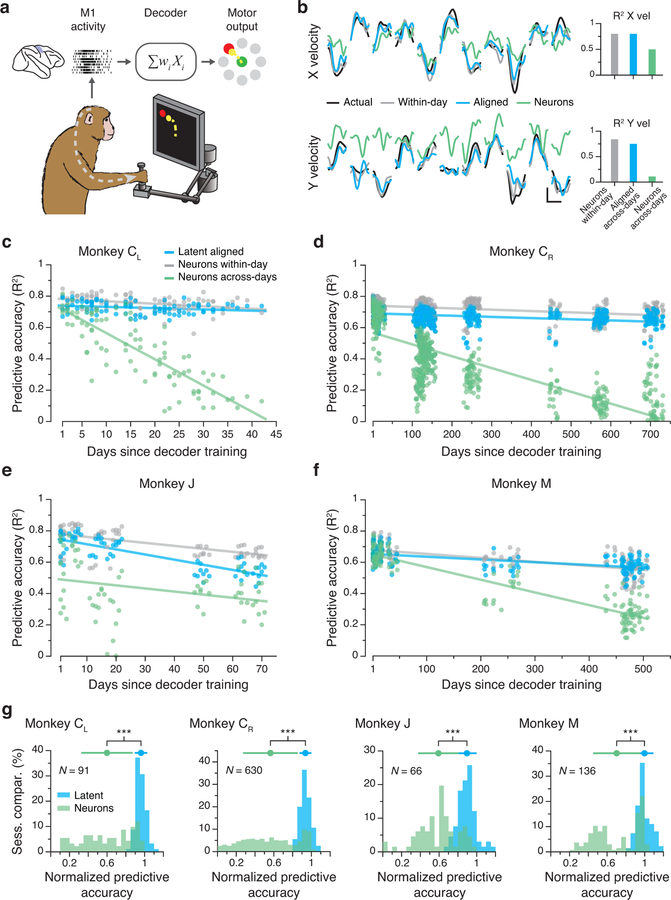
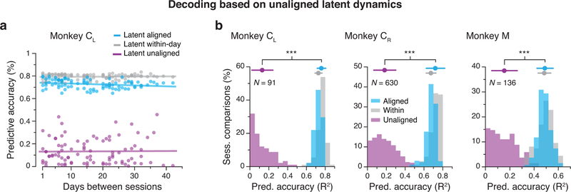
Neuroscientists often attempt to understand the information encoded within neural populations by predicting relevant behavioral features from neural activity. This is of particular interest within the field of brain-computer interfaces (BCIs) that seek to “decode” cortical activity to obtain control signals for computer cursors, robots, or prostheses that reanimate paralyzed limbs^23–25. The limited stability of these decoders over time has been an ongoing source of concern^11,26. Consequently, we asked how accurately a linear decoder trained to predict hand kinematics based on latent dynamics from one day would perform on aligned latent dynamics from a different day (Fig. 5a; Methods). Fig. 5b shows hand velocity reliably predicted 16 days later. This decoder nearly achieved the performance of a within-day decoder, trained and tested on data from the same session, and clearly outperformed both decoders based directly on the recorded multiunit neural activity (Fig. 5b) or on the unaligned latent dynamics (Extended Data 6). This observation held for all pairwise comparisons of days (Fig. 5c). We obtained similar results for the other three M1 implants (Fig. 5d–f), even for data taken over two years. To summarize these comparisons, we computed a normalized predictive accuracy: the ratio of the across-day to within-day R² (Fig. 5g). This analysis demonstrated that decoders based on the aligned latent dynamics predict behavioral features almost as well as those trained on same day neural recordings, a performance stability maintained over very long timespans.

Figure 5.

Stable decoding of movement kinematics based on the aligned latent dynamics. (a) We trained linear decoders to predict movement kinematics based on different types of inputs. (b) Example velocity predictions for two recordings made 16 days apart. Predictions based on the aligned latent dynamics were almost as good as predictions based on the recorded neural activity when trained and tested on the same day (bars on the right show the R² for the entire day). Scale bars: horizontal, 300 ms; vertical, 10 cm/s. (c) Predictive accuracy for decoders trained and tested on all pairwise combinations of days (single dots: pairs of days; lines: linear fits). Decoders based on the aligned latent dynamics (green) performed almost as well as decoders trained and tested on the same day (gray), and much better than decoders trained on the recorded neural activity when tested across days (blue). (d)-(f) Same as (c) for the other three M1 implants. (g) Normalized predictive accuracy for fixed decoders based on the aligned latent dynamics (green) and the recorded neural activity (blue), both tested on a different day. Each panel shows one monkey; each data point is one pairwise comparison between different days. The mean normalized predictive accuracies of decoders based on aligned latent dynamics are close to 1 for all monkeys; this indicates that they are nearly as predictive about behavior as same-day decoders. *** indicates P < 0.001, two-sided Wilcoxon rank-sum test. Error bars: mean ± s.d. N: number of across-day comparisons.

Stable latent dynamics are not a byproduct of neural tuning to movement

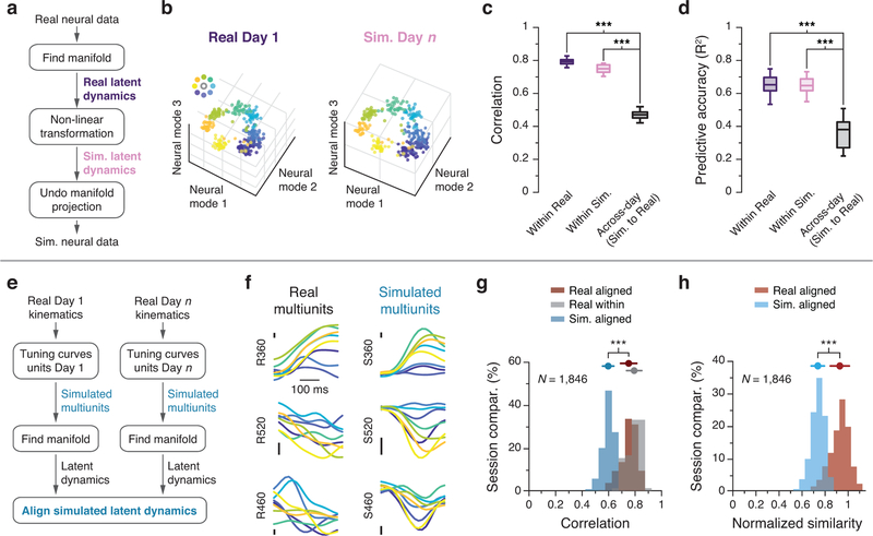
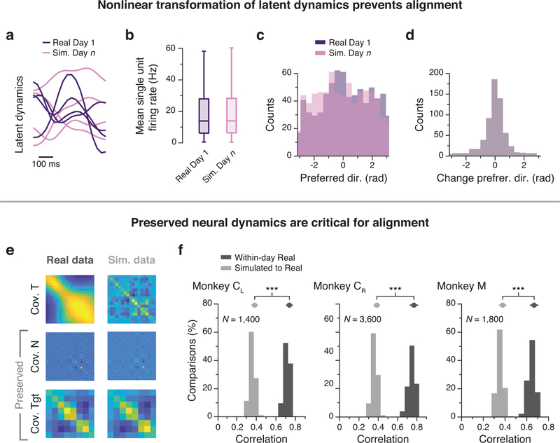
An important remaining question is whether the observed stability in the latent dynamics could be a byproduct of simpler phenomena. To test this possibility, we performed several control simulations. First, we created a surrogate dataset whose latent dynamics were nonlinearly related to the actual latent dynamics of each day (Fig. 6a; see Methods, and examples in Extended Data 7a). The surrogate neural activity preserved key features of the actual activity across the population (Extended Data 7b–d) and the target-specific clustering of within the neural manifold¹³ (Fig. 6b). Yet, this nonlinear transformation significantly decreased both alignment by CCA (Fig. 6c) and decoding of movement kinematics (Fig. 6d) across days, despite comparable within-day correlations and predictions. We observed a similar decrease in CCs when using the Tensor Maximum Entropy (TME) method² to generate a surrogate neural population. Like our first control, TME distorts the relation between neural and behavioral dynamics, yet it preserves the covariance across neurons as well as across reach conditions, thereby maintaining a measure of the neurons’ directional tuning (Extended Data 7e,f; see Methods). Thus, successful alignment with CCA, such as we observed across days in our M1 data (Fig. 4,5), requires linearly stable latent dynamics.

Figure 6.

Control analyses establish the importance of latent dynamics. (a) We created surrogate population activity by applying a nonlinear transformation to the latent dynamics of the recorded neural data and projecting them back onto the neural space (see Methods). (b) Both real and surrogate population activity exhibited target-specific clustering within the manifold. Each point represents the average activity during a reach in one session from Monkey C_L. (c) Across all sessions from Monkey C_L, CCs between the populations (black) were lower than CCs within the real (dark purple) and surrogate (light purple) populations. Box plots show median and 25^th/75^th percentiles, whiskers show range. N=14 sessions. (d) Decoders trained using real population activity performed poorly on the surrogate dataset, even after alignment. (e) We simulated population activity on two different days by passing movement kinematics of each day through tuning curves fit to the neural data of that day. (f) Example firing rates aligned to movement onset for real and simulated multiunit activity. Traces are colored by target as in (b). Vertical scale bar: 2 Hz. (g) Across all sessions from all M1 implants, canonical correlations between simulated latent dynamics (blue) were lower than those obtained from the actual latent dynamics from the same two days (red); the within-day CCs (gray) provide an upper bound. (h) Normalized similarity of the real latent dynamics (red) and of the simulated latent dynamics (blue). *** indicates P < 0.001, two-sided Wilcoxon rank-sum test. Error bars: mean ± s.d. N: number of simulated-to-real comparisons.

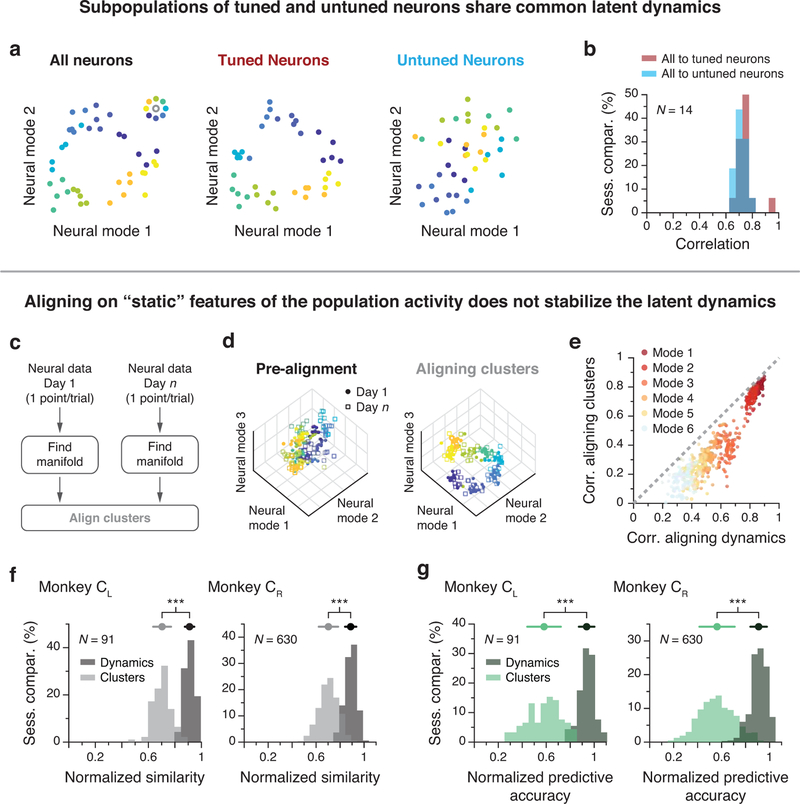
We also asked whether the observed stability of the latent dynamics could arise from movement tuning alone. We fit a speed-dependent cosine tuning curve (Methods) to each neuron recorded on Day 1, and separately to each neuron recorded on Day n. We then simulated the activity of these two surrogate neural populations by passing the recorded movement kinematics for each of these two days through the corresponding tuning curves (Fig. 6e,f). If stable single-neuron tuning curves were sufficient to explain our observed long-term stability, CCA should bring the dynamics of the two simulated populations into good alignment. However, alignment of the simulated data (Fig. 6e) resulted in significantly lower CCs than those for the real data (Fig. 6g,h). This result establishes that the real neural population activity involves a degree of dynamical stability that is not a trivial consequence of stable movement tuning at the population level. Additional control analyses shown in Extended Data 8 further illustrate the insufficiency of movement tuning (Extended Data 8a,b) and the necessity of precise temporal dynamics for alignment (Extended Data 8c–g; see Methods). Together, these quantitative controls demonstrate that although tuning properties of individual units result in some degree of alignment, this single-neuron property is not sufficient to match the degree of latent dynamics alignment found in the real data.

Dorsal premotor cortex during movement planning

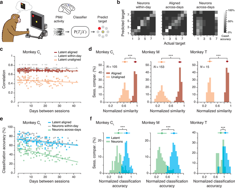
We next asked whether we might also observe stable latent dynamics in PMd activity during motor planning (Fig. 7a). Pre-movement planning activity in PMd captures many features of the subsequent behavior, including reaction time²⁷ and even the ability to learn²². We thus expected that consistent behavior would be preceded by stable motor planning dynamics. We tested the stability of PMd latent dynamics during planning using the same CCA alignment procedure we used for M1 latent dynamics. As was the case for M1, despite changes in recorded neurons (example in Extended Data 9a; see also Extended Data 3,4), PMd latent dynamics for three monkeys were stable over weeks to months to a degree nearly indistinguishable from that of within-day dynamics; in comparison, the unaligned across-days latent dynamics were quite different (Fig. 7c,d, Extended Data 9b,c).

Figure 7.

Stability of PMd latent dynamics during movement planning. (a) We trained classifiers to predict the intended target based on neural activity. (b) Example confusion matrices showing classification performance. Within-day classifiers (left) performed well (73% correct). The performance of across-day classifiers (middle) based on the aligned latent dynamics was well above chance (54%), while classifiers based on recorded neural activity (right) performed poorly (23%) when trained and tested on different days. Gray scale: classification accuracy. (c) Average correlations for aligned (CCs; red) and unaligned (Pearson’s r; orange) PMd latent dynamics across all pairs of days from Monkey C_R compared to within-day correlations (gray). Dots: pairs of days; lines: linear fits. (d) Normalized similarity of the PMd latent dynamics during movement planning for each monkey. A value of one indicates that the dynamics are as correlated as within-day. N: number of across-day comparisons. (e) Classification accuracy for classifiers trained and tested on all different pairs of days. Classifiers based on the aligned latent dynamics (green) performed almost as well as classifiers trained and tested on the same day (gray), and much better than classifiers trained and tested on different days (blue). (f) Normalized predictive accuracy for classifiers using aligned latent dynamics (green) and recorded neural activity (blue) tested on a different day. The mean normalized accuracies of the aligned classifiers are near one. *** indicates P < 0.001, two-sided Wilcoxon rank-sum test. Error bars: mean ± s.d. N: number of across-day comparisons.

We then tested whether these stable latent dynamics in PMd could be used to predict behavior. Previous work showed that the intended target of a movement can be predicted from the PMd planning activity before it occurs²³. We used naïve Bayesian classifiers¹³, trained on either the full population activity or the aligned latent dynamics, to predict the upcoming reach target during the preparatory period before movement began (Fig. 7a; Methods). We compared the across-day performance of this classifier to that of classifiers trained and tested within-day. For Monkey C_L, the across-day classifier based on aligned latent dynamics maintained high accuracy (Fig. 7b,e, Extended Data 9d,e). In contrast, fixed classifiers show a steady, progressive performance decline when used with unaligned inputs (Fig. 7e, Extended Data 9d,e), The normalized classification accuracy – the ratio of the across-day accuracy to the within-day accuracy – shows that the aligned across-day classifiers predict nearly as well as the within-day classifiers for all three monkeys (Fig. 7f), providing further evidence that stable latent PMd dynamics underlie consistent behavior.

Primary sensory cortex during feedback control

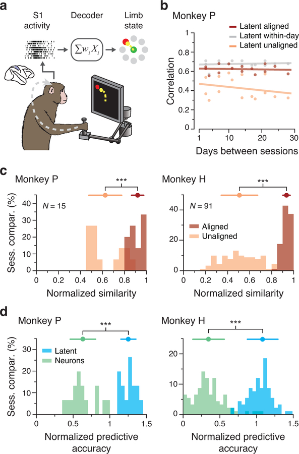
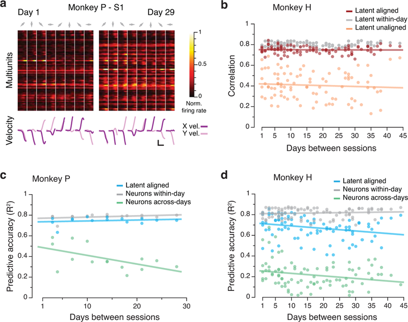
A third important aspect of the neural control of movement is the integration of sensory feedback. Proprioception, our sense of body positioning and movement, is critical for motor control, as shown by the deficits in movement coordination exhibited by patients with impaired proprioception²⁰. Here, we examine area 2 of primary somatosensory cortex (S1), a proprioceptive part of the brain that integrates feedback from cutaneous and muscle receptors^18,19. Given the stability of latent dynamics during planning and execution in PMd and M1, we anticipated seeing similar stability in the activity of S1. Using S1 data recorded during reaching (Fig. 8a, Extended Data 10a), we found that latent dynamics in S1 for two different monkeys were stable up to ~45 days (Fig. 8b, Extended Data 10b). As with the other cortical regions, the normalized stability of the aligned latent dynamics was near the upper bound set by the within-day correlations of latent dynamics (Fig. 8c).

Figure 8.

Stability of S1 latent dynamics during feedback control. (a) We trained decoders to predict movement kinematics from S1 activity. (b) Average correlation of aligned (CCs; red) and unaligned (Pearson’s r; orange) S1 latent dynamics for all pairs of days from Monkey P (single dots: pairs of days; lines: linear fits). The aligned latent dynamics have higher correlations across days than the unaligned dynamics, almost as high as within-day (gray). (c) Normalized similarity of the aligned (red) and unaligned (orange) S1 latent dynamics. N: number of across-day comparisons. (d) Normalized predictive accuracy for decoders based on the aligned latent dynamics (blue) and recorded neural activity (green) when tested on a different day. *** indicates P < 0.001, two-sided Wilcoxon rank-sum test. Error bars: mean ± s.d. N: number of across-day comparisons.

We lastly tested whether the relationship between aligned latent dynamics and hand velocity was stable over time, using decoders similar to those used for M1 (Fig 8a; Methods). Decoders based on the aligned latent dynamics provided stable predictions for both monkeys (Fig. 8d, Extended Data 10c,d). As was the case for the motor cortical regions, the accuracy of these predictions was similar to that of decoders trained and tested on the same day (Fig. 8d, Extended Data 10c,d). In contrast, the performance of fixed decoders based on recorded neural activity rapidly degraded across days. These results suggest that stable behavior is associated with stable latent dynamics throughout sensorimotor cortex.

DISCUSSION

Once learned, behaviors can be readily executed accurately and consistently. How the brain achieves this behavioral stability is still an open question. Existing readouts of neural activity have been fraught with the problem of ever-changing neurons, making it extremely difficult to answer questions about the long-term stability of cortical dynamics. Here we showed that repeated execution of a given behavior is accompanied by latent dynamics in several cortical sensorimotor areas that remain stable over remarkable lengths of time. These stable latent dynamics are associated with three main aspects of movement generation²⁸: planning the upcoming movement, controlling its execution, and integrating somatosensory information. Moreover, the stabilized latent dynamics maintained a fixed relationship with the behavior: decoders based on the stabilized latent dynamics are able to predict behavior up to two years after training, almost as well as decoders tested on the same day as they are trained.

While skilled movements can be remarkably consistent over a long time, prior studies disagree on the stability of movement information in single neurons over short periods of time (from one to four days), with some claiming inherent instability of tuning properties²⁹ and others claiming stability well within the error introduced by measurement noise^11,17,30. However, none of these studies attempted to address changes in neural activity due to changing neural recordings, an intrinsic feature of multielectrode array recordings over extended periods (Fig. 3b,c, Extended Data 2, 3, 4, 9, 10). How can we find stable latent dynamics based on unstable neural recordings³¹? Here we assume that the dynamics of cortical neurons are confined to a low-dimensional manifold¹ (Fig. 1c). On each recording day, we can only obtain an empirical estimate of the latent dynamics. Our results show that these empirical estimates vary greatly across days. However, our ability to align these dynamics supports the view that the true latent dynamics are stable when a given behavior is repeated. The differences across days arise from projecting the true latent dynamics onto the changing empirical neural spaces that are determined by the neural recordings. This projection involves two linear transformations. First, the true latent dynamics within the full neural space – which incorporates all neurons modulated by the task – are projected onto the empirical neural space of the recorded neurons. This transformation involves a dimensionality reduction from at least 10⁶ to 10². Then, the manifold embedded within the empirical neural space is found; this transformation involves a dimensionality reduction from approximately 10² to 10¹ for the relatively simple reaching behaviors we and others have studied⁸. Since both of these operations are linear, it is not surprising that the latent dynamics alignment can be achieved with a linear method such as CCA. Given the ubiquity of linear analyses such as PCA in modern neuroscience experiments, our observation has important implications for understanding how neural populations throughout the brain consistently perform behaviorally relevant functions.

There remains the concern that CCA might be too powerful and could potentially find transformations that make unstable true latent dynamics appear stable. We argue against this scenario. A nonlinear change in the intrinsic dynamics of the network would reduce the magnitude of the CCs attainable by alignment, as illustrated by our “nonlinear transformation” control analysis (Fig. 6a–d, Extended Data 7a–d). In contrast, CCA should be able to compensate for any linear transformation to the latent dynamics. While this necessarily includes the transformation resulting from changing neural recordings, there is still the possibility of additional linear transformations acting on individual neurons and resulting in linear changes in the true latent dynamics in the period between the two days being compared. Given the intrinsically nonlinear properties of neural networks^6,21 composed of nonlinear neurons connected by nonlinear synapses, it is difficult to assess either the likelihood or the behavioral relevance of such a linear transformation.

Our results emphasize the importance of low-dimensional neural population dynamics, a concept that has furthered our understanding of computation in the brain^1,9. However, we should always question whether the observed properties could be an byproduct of simpler phenomena². We asked whether the results reported here could be explained by movement tuning properties of individual neurons. The control analyses and simulations (see Fig. 6, Extended Data 7,8) reveal that although tuning properties of single neurons result in some degree of alignment and decoder stability, they are insufficient to explain the degree of stability that we observed in the real neural data. There is also an important conceptual point: even if alignment could be improved through more sophisticated tuning models, this single-neuron approach will remain incomplete. The attempt to explain our stability results on the basis of movement-tuned neurons implies a computational view of the population as an ensemble of independent units, each endowed with a tuning curve. In this view, covariance between two neurons can only arise because similarities (or oppositions) between their tuning curves yield correlated (or anticorrelated) activity. This picture is necessarily incomplete, and leads to an underestimation of covariances that also arise because of common inputs, and, more importantly, actual connectivity³². Our analyses demonstrate that the contribution of these factors to behaviorally relevant latent dynamics cannot be ignored. Recent work has established that the collective dynamics of neural populations are strongly influenced by network connectivity^33–35, and that long-term learning is needed to alter or extend the manifold^3,22,36. We posit that a view of neural activity that ignores interactions between neurons and attempts to explain all pairwise correlations on the basis of their individual tuning curves is bound to be incomplete and thus insufficient to fully explain population dynamics.

It is important to note that we studied the neural dynamics underlying the planning and execution of a single, stereotyped reaching behavior. The corresponding neural dynamics are intimately and necessarily linked to this behavior. A different behavior, such as shaking a cocktail shaker, would require its own dynamics, though a comparative analysis of these two different behaviors might reveal some similarities. The extent to which latent dynamics are shared between behaviors is an area of active investigation. A recent study from our lab has shown both shared and behavior-specific components in M1 latent dynamics when comparing different but related wrist movement and reach-to-grasp tasks⁵. Another study in mice has shown greater differences in M1 dynamics between forepaw reaching and quadrupedal locomotion³⁷. These observations raise the concern that the stable latent dynamics we describe may trivially arise from our use of a consistent behavior. However, simulation work by Sussillo et al. provides an interesting argument that even consistent behavior is not necessarily associated with stable latent dynamics²¹. They trained recurrent neural networks (RNNs) to reproduce muscle activity (EMG) recorded during reaching. The network architecture had to be regularized to obtain good CCs between the simulated and actual latent dynamics; without this constraint, CCs were low, even though the RNN accurately reproduced the EMG²¹. The consistent behavior, in this case represented by the EMG, was not necessarily associated with stable latent dynamics within the RNN. Given the convergence between motor cortex and spinal motoneurons, it is unsurprising that the neural dynamics associated with a particular behavioral output need not be unique. Additionally, the latent dynamics in PMd are stable during motor planning, when no behavior has yet occurred. We thus propose that the stability of latent dynamics reported here is not a trivial consequence of the consistent behavior, but rather reflects a fundamental feature of learned cortical function that leads to stable behavior.

Our results have important implications for BCIs that map neural activity onto control signals and promise to revolutionize rehabilitation and assistive technologies³⁸. Many labs have used BCI decoders to control computer cursors²³, robots²⁵, and even reanimate paralyzed limbs through electrical stimulation²⁴. However, the neural activity that provides inputs to these decoders typically changes over weeks and months, leading to degraded BCI performance^39,40. Some groups have suggested that the use of local field potentials^41,42 could reduce the magnitude of these changes, at the risk of reducing the amount of information available to the decoder. Other groups have been developing computational techniques to continually recalibrate these decoders and restore degraded function⁴³. While feasible, decoder recalibration may impose an undesirable cognitive burden on the user when compared to stabilizing the inputs to a fixed decoder. The stable latent dynamics reported here offer an intriguing alternative to previous approaches that attempted to align the statistics of neural activity^44,45: decoders based on latent dynamics could be periodically aligned through a linear procedure such as CCA, thereby achieving stable performance for years. Recent work has further shown that population-based approaches can improve decoding stability^6,26,46, enable unsupervised decoding⁴⁴, or even adjust for changes in neural activity based on its statistics alone⁴⁵.

We have reported here on the stable latent dynamics in three cortical areas that are closely tied to the resulting behavior²⁸. We posit that the stability of the behavior and the stability of the corresponding latent dynamics are intimately tied to each other. However, the population dynamics associated with a specific behavior differ across brain areas^22,47, and thus could appear less stable in brain areas that are upstream from those studied here. For example, decision-making dynamics in prefrontal cortex depend on the resulting behavior, but also on internal states (e.g., arousal) and sensory inputs (e.g., visual) that influence the behavioral decision. There could thus be different neural dynamics that reflect changes in internal state but underlie a stable behavioral output. Within the motor cortex, recent work indicates that the supplementary motor area, a “higher” motor cortical area whose activity reflects motor timing⁴⁸ or sequence production⁴⁷, exhibits more complex dynamics than what is consistently observed in M1⁴⁷. Perhaps the dynamics of such areas are less stable over long spans of time, as their activity captures more than the observable behavioral output. Still, our results support the hypothesis that when the activity of a brain area is intimately tied to a behavioral output, the underlying latent dynamics corresponding to stable behavior are preserved.

In conclusion, we have shown that the latent dynamics associated with the consistent execution of a given behavior can be stable for up to two years. This observation has broad implications for experiments studying neural activity over time: the activity of individual neurons is best viewed as a sample of underlying true latent dynamics^1,7,8. Similar latent dynamics have been identified in many cortical regions (see reviews in Refs. 1,9), and for a wide variety of functions, including working memory, decision making, visual, olfactory, and auditory discrimination, navigation, and movement. Moreover, these latent dynamics exhibit some common characteristics across cortical regions^5,49 and even across species^16,50. These commonalities suggest that the stabilization of latent dynamics may be ubiquitously exploited throughout the brain. Dimensionality reduction to uncover latent dynamics is increasingly accepted as a useful method for systems neuroscience research, as the low-dimensional manifold is more amenable to analysis and visualization than the full neural space. Here, we have provided evidence that latent dynamics are not merely a convenient mathematical abstraction for model building, but the extant and stable building blocks of consistent behavior.

METHODS

Behavioral task

We trained six monkeys to sit in a primate chair and make reaching movements using a custom planar manipulandum. All six of the monkeys performed a similar two-dimensional center-out task (Fig. 2a) for long periods of time; across all monkeys we collected 137 days of data, across timespans between three weeks and approximately two years. In the task, the monkey moved his hand to the center of the workspace to begin each trial. After a variable waiting period, the monkey was presented with one of eight outer targets (or four targets for Monkey H), equally spaced in a circle and selected randomly with uniform probability. Monkeys C, M, and T were trained to hold during a variable delay period during which the target remained visible before receiving an auditory go cue. Monkeys P and H were not subjected to this delay period. Early recordings from Monkey C also omitted this instructed delay period, though he was later trained on the delayed version of the task. With respect to our main results, we saw no difference between these groups of sessions. To receive a liquid reward, the monkeys were required to reach the outer target within 1 s. Monkeys C, M, and T were required to hold within that outer target for 0.5 s. For Monkey P and early sessions with Monkey H, this outer target hold period was omitted. Monkey H was later subject to a brief hold period of 100 ms, to ensure that he decelerated to end the reach within the target. Thus, there were some kinematic differences between the early and later sessions with Monkey H; since much of the movement was similar, we observed similar results even when all of the recordings and all sessions were considered. Monkey C initially performed the task using the left hand; later, he used the right hand during experiments with multielectrode arrays implanted in the opposite hemisphere (C_L and C_R). As the monkeys performed this task, we recorded the position of the endpoint at a sampling frequency of 1 kHz using encoders in the joints, and digitally logged the specific timing of task events such as the go cue.

Behavioral data analysis

In all of the following analyses, we considered only the trials in which the monkey successfully achieved the outer target within the specified time and received a reward. We then sub-selected trials such that all sessions contained an equal number of reaches in each of the target directions. Within each trial, we isolated a window of interest that captured the majority of the movement. Comparison of the dynamics requires each trial on each day to have the same number of data points. We thus adjusted this window slightly according to the behavioral idiosyncrasies (reaching speed, etc.) of each monkey, so as to maximize the number of samples while preserving an equal number of data points across trials. For example, monkeys with naturally slower reach speeds were assigned longer windows. Our results were qualitatively unchanged with reasonable adjustments to this window. For Monkeys M, T, C, and J we used a window starting 120 ms before movement onset and ending 420 ms after movement onset. For Monkeys P and H, we used windows beginning at the go cue and ending after 570 ms or 660 ms, respectively.

We performed all subsequent analyses by comparing all pairs of sessions performed by each monkey, only looking forward in time. For example, with three days of recordings, we compared Day 1 to Day 2, Day 1 to Day 3, and Day 2 to Day 3. In general, when a recording on Day j was compared to a subsequent recording on Day n,the result was assigned to $\left(n-j\right)$ days between sessions. First, we studied the hand kinematics to assess behavioral consistency. We took the derivative of the endpoint position to compute the endpoint velocity. Within each session, we ordered all trials by reach direction and concatenated all trials. Since the trials were sub-selected to equalize the counts across both time and reach directions (last column of Supplementary Table 1), the resulting data matrices were of equal size for all days. Each matrix entry represented a datapoint from the same time sample and target across all days, allowing for a point-by-point direct comparison of dynamics. To assess the stability of behavior over time, we computed the correlation (Pearson’s r) for the 2-D velocity signals between pairs of days in all possible combinations.

Neural implants

All surgical and experimental procedures were approved by the Institutional Animal Care and Use Committee (IACUC) of Northwestern University. In order to record chronically from populations of cortical neurons, we implanted 96-channel Utah electrode arrays in M1, PMd, or S1 using standard surgical procedures. Monkeys T (male, macaca fascicularis) and M (male, macaca mulatta) were implanted in PMd of the right hemisphere; Monkey M also received a second array in right M1 in the same procedure. Monkey C (male, macaca mulatta) received two implants: first, a single array in right M1 (denoted C_R throughout the text), followed years later by implants in both M1 and PMd of the left hemisphere (denoted C_L). Monkey J (male, macaca mulatta) received an array in the left M1. Both Monkeys P and H (male, macaca mulatta) received arrays in S1 (Brodmann’s Area 2) of the left hemisphere. Supplementary Table 1 summarizes the implants and sessions of neural recordings for each monkey.

Neural activity was recorded during the behavior using a Cerebus system (Blackrock Microsystems, Salt Lake City, UT). The recordings on each channel were digitized, band-pass filtered (250–5000 Hz), and then converted to spike times based on threshold crossings. The threshold was set according to the root-mean square (RMS) activity on each channel (Monkeys C, M, T, and J: 5.5×RMS; Monkey P: 4×RMS; Monkey H: 5×RMS). Although most of the analyses of this paper focus on the multiunit threshold crossings on each recording channel, we also manually spike-sorted the recordings from Monkeys M, C, and T to identify putative single-neurons, which we used in the control analyses for M1, as well as in the tracking across days analysis (see below).

Tracking single neurons over days

For all sessions recorded with Monkeys C, M, and T, we sorted the waveforms that exceeded the threshold to identify putative single neurons. Each of these sorted units can be uniquely described by its waveform shape and its inter-spike interval (ISI) distribution. We applied a statistical test based on these metrics to determine whether or not a given neuron was recorded on two different days¹⁰. In brief, the waveform shape and ISI of two neurons recorded on a given electrode on two different days was compared against a null distribution taken from neurons recorded on all other electrodes, thus known to be from different neurons. Cells were considered to match if the joint probability of both metrics matching was less than 0.01.

Analysis of neural spatial tuning across days

We described the spatial tuning of the multiunit activity recorded by each electrode using cosine tuning curves^51–53. On each recording electrode, we computed the average firing rate within the time window used for decoding or classification (during motor execution for M1 and S1, and during motor planning for PMd, respectively). On each session, we then averaged across all trials for each reach direction and used linear regression to fit the tuning curve according to:

$$f=b+a\cos \left(\theta -{\theta }^{*}\right),$$

where b is the baseline mean firing rate, a is the depth of modulation, and ${\theta }^{*}$ is the preferred direction⁵¹; these three parameters describe the directional tuning of the average firing rate f for each recording electrode. For each electrode, we tracked the changes in the parameters of this model across all pairs of days for which neural activity was recorded on that electrode on both days. For this subset of electrodes, we assessed the magnitude of the change in mean firing rate, modulation depth, and preferred direction, the latter as a circular difference.

Neural latent dynamics analysis

To characterize the dynamics of the latent activity associated with the recorded neural activity in each session, we computed a smoothed firing rate as a function of time for the multiunit activity on each electrode. We obtained these smoothed firing rates by applying a Gaussian kernel (s.d.: 50 ms) to the binned square-root-transformed firings (bin size: 30 ms) of each recorded multiunit⁵⁴. We excluded electrodes whose activity had a low mean firing rate (< 1 Hz mean firing rate across all bins), but did not perform any additional preselection, such as based on directional tuning. For each session, this produced a neural data matrix X of dimension n by T, where n is the number of recorded units and T is total number of time points from all concatenated trials on a given day; T is thus given by: number of targets per day × number of trials per target × number of time points per trial. We performed this concatenation as described above, by subselecting the same number of trials for all sessions and targets for each monkey (Supplementary Table 1) and ordering the datapoints by time and target. For the analysis of M1 and S1 activity, we considered the same window of interest during a trial as we did for the behavioral analysis (see above); these values were chosen to represent movement execution in M1, and feedback control in S1. For the PMd activity, we analyzed the preparatory activity within a window aligned with movement onset, starting 390 ms before movement onset, and ending 60 ms after movement onset. This window started after the putative visual response elicited by the target presentation^12,55, and it was advantageous because it included mostly preparatory activity, but also some of the dynamics of the transition from preparation to movement.

For each session, the activity of n recorded multiunits was represented as a neural space, an n-dimensional sampling of the neural space of the cortical area of interest. In this space, the joint recorded activity is represented as a single point whose coordinates are determined by the firing rate of the corresponding multiunits (see, e.g., Fig. 1d). Within this space, we computed the low-dimensional manifold by applying principal component analysis (PCA) to the neural data matrix X. This yielded n principal components (PCs), each a linear combination of the smoothed firing rates of all n recorded units. These PCs are ranked based on the amount of neural variance they explain. We defined an m-dimensional session-specific manifold by keeping only the leading m PCs, which we refer to as neural modes (Fig. 1d). Based on previous work by our group and others, we chose the following dimensionality values: m=10 for M1, m=15 for PMd, m=8 for S1. The specific choice of m is not critical, as our results held across a broad range of m values (Extended Data 5a–c).

We computed the latent dynamics within the manifold by projecting the time-dependent smoothed firing rates of the recorded neurons onto the PCs that span the manifold. This produced a data matrix L of dimensions m by T, where m is the dimensionality of the manifold and T is total number of time points from all concatenated trials on a given day. Recent theoretical and experimental work has demonstrated that when the recorded neural activity is projected onto the low-dimensional manifold to obtain the latent dynamics, the result is not sensitive to whether the manifold was estimated on the basis of single units or multiunits⁷. Nevertheless, we repeated all the analyses for a subset of three monkeys with M1 implants by using putative single neurons to obtain the manifold, and verified that our results held (Extended Data 5d,e).

Alignment of latent dynamics across days

The substantial turnover across days observed in our neural recordings (Extended Data 3, 4) implies that the neural space in which the experimentally accessible manifold and the latent dynamics are embedded changed across days. Our hypothesis predicts that the true latent dynamics associated with consistent behavior should be stable across days. In order to verify this hypothesis, we need to compensate for the fact that the true latent dynamics is being projected onto different manifolds on different days. If our hypothesis is correct, we expect to be able to compensate for this change in the embedding space by using canonical correlation analysis^5,21,56 (CCA). Given the concatenated single-trial latent dynamics ${\text{L}}_A$ and ${\text{L}}_B$ from two days A and B, CCA finds linear transformations that applied to ${\text{L}}_A$ and ${\text{L}}_B$ make the corresponding latent dynamics maximally correlated.

CCA starts with a QR decomposition of the transposed latent dynamics matrices ${\text{L}}_A$ and ${\text{L}}_B$, ${\text{L}}_A^{\text{T}}={\text{Q}}_A{\text{R}}_A$,${\text{L}}_B^{\text{T}}={\text{Q}}_B{\text{R}}_B$. The first m column vectors of ${\text{Q}}_i, i=A,B$, provide an orthonormal basis for the column vectors of ${\text{L}}_i^{\text{T}}, i=A,B$. We then construct the m by m inner product matrix of ${\text{Q}}_A$ and ${\text{Q}}_B$ and perform a singular value decomposition to obtain

$${\mathbf{\text{Q}}}_A^{\text{T}}{\mathbf{\text{Q}}}_B={\mathbf{\text{U S V}}}^{\text{T}}$$

CCA finds new manifold directions to maximize the pairwise correlations across the two days. The projection of the latent dynamics onto these new manifold directions are implemented through the corresponding m by m matrices

$$M_A=R_A^{-1}U, M_B=R_B^{-1}V$$

These transformations result in latent dynamics projected onto new manifold axes,

$${\tilde{\mathit{L}}}_A^{\text{T}}={\mathbf{\text{L}}}_A^{\text{T}} M_A, {\tilde{\mathit{L}}}_B^{\text{T}}={\mathbf{\text{L}}}_B^{\text{T}} M_B.$$

The CCs between the unaligned latent dynamics are the pairwise correlations between the rows of ${\mathbf{\text{L}}}_A$ and ${\mathbf{\text{L}}}_B$, given by $L_A L_B^T$. The CCs after alignment are the pairwise correlations between the rows of ${\tilde{L}}_A$ and ${\tilde{L}}_B$, given by ${\tilde{L}}_A {\tilde{L}}_B^T= U^T{Q}_A^T Q_B\mathbf{\text{V = S}}$. The elements of the diagonal matrix S are the resulting canonical correlations (CCs), sorted from largest to smallest; they quantify the similarity in the aligned latent dynamics. To provide stable input to a decoder, the latent dynamics of day B are aligned to those of day A by ${\mathbf{\text{L}}}_B^{\text{T}} M_B {\left(M_A\right)}^{-1}$.

We used the within-day variability in the latent dynamics across blocks of trials for a given day to obtain an upper bound for the across-day CCs. We split all the trials in one day into two non-overlapping sets of trials, ensuring that the groups were matched by target and time points, and performed CCA on the latent dynamics (100 repetitions). The mean value for each of the top four of the ordered CCs in this distribution was used to define the within-day CCs. To represent more compactly how the alignment process compensates for the changes in latent dynamics due to neural turnover and its resultant change in embedding space, we computed the normalized similarity, the ratio of the across-day aligned or unaligned CCs to the upper bound provided by the within-day CCs.

Decoding hand velocity from motor and somatosensory neural activity

To test whether the aligned latent dynamics in M1 and S1 maintain movement-related information, we built linear decoders to predict the two-dimensional hand velocity from neural data. Our hypothesis was that the aligned latent dynamics should provide accurate predictions of hand kinematics over time. To test this hypothesis, we compared the predictive accuracy of three different types of decoders: 1) a within-day neural decoder trained and tested on the same day based on the recorded neural activity, 2) an across-day neural decoder trained on the neural activity recorded on the first day and tested on neural activity recorded on subsequent days, and 3) an across-day latent decoder trained on the latent dynamics of the first day and tested on the aligned latent dynamics of subsequent days.

All decoders were standard Wiener filters⁵⁷ that used as inputs the neural activity, either the multiunit firing rates for the within-day and across-day neural decoders or the across-day aligned latent dynamics. We also included three bins of recent spiking history, for a total of 90 ms. These additional neural inputs incorporate information about intrinsic neural dynamics and account for axonal transmission delays. When decoding from M1, whose activity causes the ensuing movement, the additional bins preceded hand velocity signals. When decoding from S1, whose activity is largely in response to the executed movement, the additional bins lagged behind hand velocity signals. The R² value between actual and predicted hand velocity was used to quantify decoder performance as a predictive accuracy. We built separate decoders to predict X and Y hand velocities; as their performances were similar, we report their mean.

The within-day decoder was trained and tested on the same session, using a six-fold cross-validation procedure to protect against overfitting. Before splitting the recorded neural activity for the session into six blocks, the corresponding trials were shuffled to remove any bias due to time through the session. The R² values for the six test blocks were averaged to obtain a final reported value. The within-day performance provided an upper-bound to the performance of across-day decoders. The across-day neural decoders were computed for all pairwise combinations of days, training on the neural activity recorded on the first of the two days and testing on the later day. The across-day aligned decoders were trained on the latent activity of the first of the two days and tested on latent dynamics of the later day after alignment. To compare across all sessions and monkeys more easily, we normalized the across-day predictive accuracy by dividing it by the within-day predictive accuracy to obtain the normalized predictive accuracy.

Predicting target direction from PMd planning activity

We trained naive Bayes classifiers to predict the direction of the upcoming movement based on pre-movement planning activity¹³. For each of the three monkeys, we used PMd neural activity recorded during a 450 ms window as inputs to the classifier (see above). This window focused primarily on the planning period before movement onset. As we did for movement prediction, we trained three types of classifiers: within-day, based on recorded neural activity, across-day based on recorded neural activity, and across-day based on aligned latent dynamics. Within the input window, we averaged all activity to obtain a single value representing the activity for that trial, resulting in either an n-dimensional neural input or an m-dimensional latent input (whether aligned or unaligned).

The naive Bayes classifiers, trained using Matlab (fitcnb), provided a probabilistic assignment of the inputs to one of eight classes, corresponding to the eight possible target directions. The predicted class was that with the maximum posterior probability. Predicted classes were assumed to be independent; hence the classifiers were naive. To ensure that all targets had the same prior probability, the training data included the same number of trials for each target.

Performance of the trained classifiers was quantified by the percentage of correct classifications. To quantify the performance of the within-day classifiers, we performed a cross-validation procedure in which we left out one random trial to each target and trained the classifier on the remaining data. We then tested the classifier on this left-out sample. We repeated this procedure 100 times and averaged the test performance. As before, we normalized the performance of the across-day classifiers by dividing it by the within-day performance to compute the normalized accuracy.

Control analyses

We constructed a scenario in which the latent dynamics are changed to prevent their alignment by CCA, while preserving the statistics of single unit properties such as mean firing rate and directional tuning across the population (Fig. 6a,b, Extended Data 7a–d). We started from Day 1 data from Monkey C_L. We computed a ten-dimensional manifold using PCA and projected the neural trajectories of Day 1 into this manifold to obtain the latent dynamics. We then artificially simulated “Day n” data with novel latent dynamics by applying a nonlinear transformation to the latent dynamics of Day 1, namely a point-by-point product of each trial’s latent dynamics with a cosine function whose period equaled the duration of the trial, to preserve the smoothness of the temporal traces. The transposed PC transformation was then used to project the simulated Day n latent activity onto the population of recorded neurons. This artificially generated population activity of Day n was then compared to the recorded activity of the neural population on Day 1 (Fig. 6c,d).

In addition, we used the Tensor Maximum Entropy² (TME) algorithm to generate surrogate datasets that share some specified set of primary features with the original neural data but are otherwise random. This control was specifically designed to investigate whether results based on population analysis can be explained by the statistical properties of single neurons alone. Here we used TME to generate surrogate populations of neurons in which the covariance across both neurons and reach conditions (a proxy for directional tuning) was preserved, but the temporal covariance associated with neural dynamics was not (Extended Data 7e). We then used PCA to obtain the manifold onto which the surrogate population dynamics were projected to obtain latent dynamics, and CCA to align the latent dynamics of the surrogate population to those of the recorded population (Extended Data 7f).

We also ran a simulation to determine the extent to which the stability of latent dynamics results from the movement tuning of individual neurons. To quantify this effect, we fit speed-dependent cosine tuning curves⁵² to the activity of each neuron recorded on Day 1, and separately to each neuron recorded on Day n. The tuning curves used in the simulation were chosen not arbitrarily, but to represent the actual neural data as closely as possible. We then generated two surrogate neural populations, one for Day 1 and one for Day n, whose activity was based on the recorded movement kinematics for those two days, passed through the corresponding fitted tuning curves (Fig. 6e; examples of surrogate neural activity in Fig. 6f). We then proceeded as in the analysis of real data: we computed the manifold of the Day 1 surrogate population and that of the Day n surrogate population and attempted to align the latent dynamics within these two manifolds using CCA. If the attempt at alignment results in significantly lower CCs than those resulting from the alignment of the real data for those two days, we must conclude that there are meaningful dynamics within the real neural population activity that facilitate alignment and are not trivially a consequence of the movement tuning (Fig. 6g,h).

We performed an additional control where each day we split the recorded neurons into two subpopulations, based on the movement tuning of each neuron (Extended Data 8a). We fit speed-dependent cosine tuning curves to the activity of each unit⁵². We then set a threshold corresponding to an R² value of 0.6 for the cosine fits across all neurons. We separated the neurons into two classes: those with R² greater than the threshold were labeled as “tuned”, and those with R² below this threshold were labeled as “untuned”. We checked whether the latent dynamics of the subpopulation of untuned units could be aligned to the latent dynamics of the whole recorded population as well as the latent dynamics of the tuned subpopulation could be (Extended Data 8b). Results were not sensitive to the actual value of the threshold used to split the units recorded on each day into “tuned’ and “untuned” subpopulations.

As a final control, we quantified the amount of correlation that could be achieved when alignment was implemented based on static properties of the neural activity associated with each reach, as opposed to the corresponding latent dynamics. To this end, we abandoned the 30 ms resolution used to track neural activity during individual trials and represented the activity of each neuron in each trial by its average firing rate in the 300 ms interval following movement onset (Extended Data 8c). For each session, this resulted in a neural data matrix X of dimension n by T, where n is the number of recorded units and T is the number of targets per day × number of trials per target, as there is only one firing rate per neuron per trial. We analyzed this data matrix as before, reducing the dimensionality from n to m = 10 using PCA, then applying CCA to align the resulting target-specific clusters across days (Extended Data 8d). We then projected the latent dynamics onto these cluster-aligned manifold axes. Similarity (correlation) and corresponding normalized similarity were computed as before (Extended Data 8e–g) and compared to those achieved when the alignment was based on the latent dynamics.

Statistics

We applied statistical tests to compare results for the across-day recorded neural activity and the across-day aligned latent dynamics. For all statistical tests, we used distributions that had been scaled by dividing by the within-day values, either for canonical correlation or decoding and classification performance. We used a two-sided Wilcoxon rank-sum test to compare the distributions, which were not necessarily assumed to be normal. Throughout all analyses we used a significance threshold of P < 0.001. No statistical methods were used to pre-determine sample sizes, though our dataset included a large number of sessions and subjects, many more than typical studies in the field. The data analysis supporting our conclusions required no experimental intervention, thus no randomization into groups was needed and the experimenters were not blinded to the nature and goals of the experiment.

Extended Data

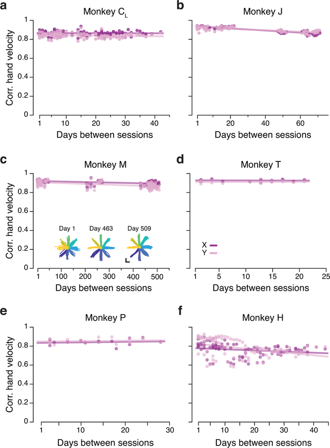
Extended Data Fig. 1. Additional data: task description and consistent behavior.

(a-f) Correlation between direction-matched single trial X and Y hand velocities across all pairs of days (single dots: individual trials; lines: linear fits) from Monkey C_L (a), Monkey J (b), Monkey M (c), Monkey T (d), Monkey P (e), and Monkey H (f). The inset in (a) shows X and Y hand trajectories for three example sessions. Trajectories are color coded by target as in Figure 2.

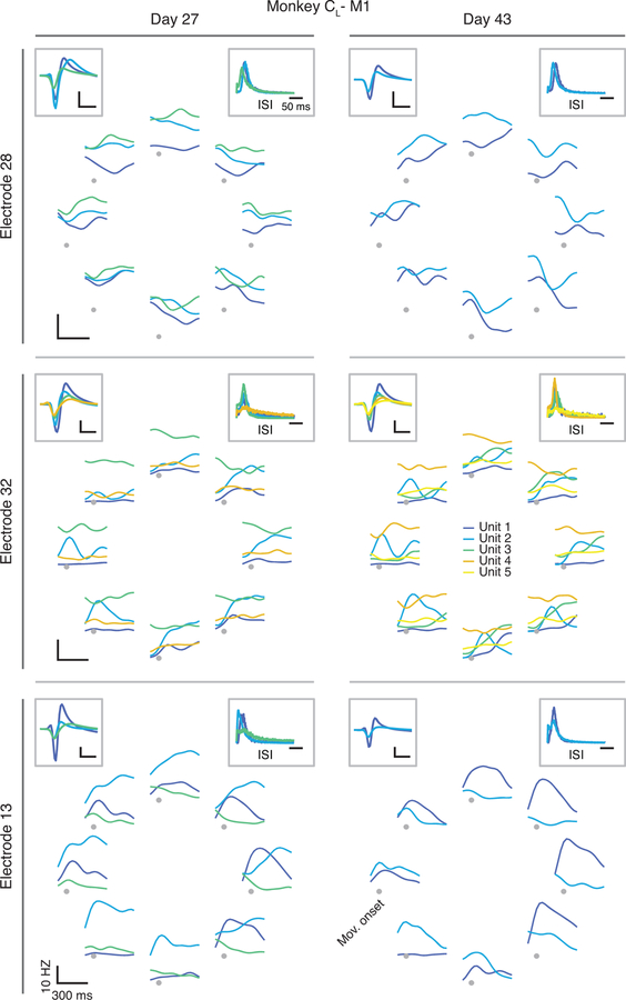
Extended Data Fig. 2. Additional data: example neural activity during reaching on two days from Monkey C_R.

Each row shows the firing rates on a different electrode for Day 27 (left column) and Day 43 (right column). Each color represents a different sorted neuron. The eight plots arranged in a circular manner show the firing rate as a function of time during a reach to each of the eight targets, aligned on movement onset and averaged across all trials to the same target. The inset in the top left of each panel shows the average waveform of each sorted neuron; the inset at the top right shows the ISI distribution for each sorted neuron. Inset scale bars: horizontal, 400 µs; vertical, 200 µV.

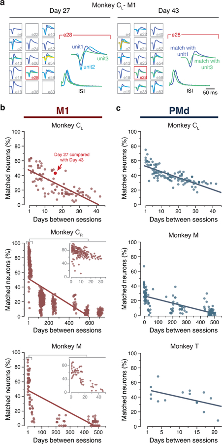
Extended Data Fig. 3. Additional data: neural recording stability.

(a) We manually spike-sorted the neural recordings from Monkeys C, M, and T to establish whether the same neurons were recorded across days (Methods; Extended Data 2 shows example neurons). Plots show the average action potential waveform of example sorted neurons for two datasets: Day 27 and Day 43 from Monkey C_L. Note the large apparent turnover after 15 days. Right insets: example action potential waveforms and inter-spike interval (ISI) histograms for two neurons that were matched across days. (b) To quantify the turnover effect, we tracked both firing rate statistics and waveform shape of each neuron; these figures show the percentage of individual sorted M1 neurons that were matched across pairs of days based on action potential waveforms and inter-spike interval (ISI) histograms. Data from Monkey C_L (top), Monkey C_R (middle; inset highlights the first 35 days), and Monkey M (bottom; inset highlights the first 50 days). (c) Percentage of individual sorted PMd neurons that were matched across pairs of days as in (a). Data from Monkey C_L (top), Monkey M (middle), and Monkey T (bottom).

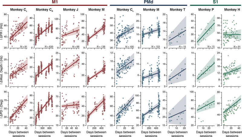
Extended Data Fig. 4. Additional data: neural tuning stability.

For each implant: change in mean firing rate (top plot), modulation depth (middle plot), and preferred direction (bottom plot) of standard cosine tuning fits to multiunit activity across all pairs of days. Line and shaded areas: mean ± s.e.m. Plots are grouped by implant and brain area (M1: left; PMd: middle; S1: right). Error bars: 95% confidence interval of linear fit. N: number of across-day comparisons.

Extended Data Fig. 5. Additional data: controls for the alignment procedure using M1 data.

(a) Correlation of the aligned (CCs; red) and unaligned (Pearson’s r; orange) M1 latent dynamics averaged over the top four neural modes across all pairs of days from Monkey C_L using a 6-D manifold (single dots: pairs of days; lines: linear fits). (b) Normalized similarity of the aligned and unaligned M1 latent dynamics in the 6-D neural manifold for Monkey C_L. (c) Mean and s.e.m. for normalized similarity distributions as shown in (b), for all four M1 implants for 6, 8, 10, and 12-D manifolds. The 10-D data presented here summarizes the distributions shown in Fig. 4. The significance of the separation between aligned and unaligned distributions held regardless of the choice of neural manifold dimensionality. N values are the same as for the corresponding distributions in Fig. 4. (d) Correlation (CCs) of the M1 latent dynamics averaged over the top four neural modes across all pairs of days from Monkey C_L using sorted neurons rather than multiunit activity (single dots: pairs of days; lines: linear fits). (e) Normalized similarity of the aligned and unaligned M1 latent dynamics in the 10-D manifold obtained using sorted neurons for Monkeys C_L, C_R, and M. Error bars: mean ± s.d. N: number of across-day comparisons.

Extended Data Fig. 6. Additional data: movement decoding-based controls for the alignment procedure.

(a) Predictive accuracy when decoding hand velocity for all pairs of days from Monkey C_L, using the unaligned latent dynamics as inputs instead of the multiunit activity used in Fig. 5. (b) Predictive accuracy when using as inputs the latent dynamics within-day, and across-day both before and after alignment, for Monkeys C_L, C_R, and M. *** denotes p < 0.001, two-sided Wilcoxon rank-sum test. Error bars: mean ± s.d. N: number of across-day comparisons.

Extended Data Fig. 7. Additional data: Altering neural temporal dynamics prevents their alignment.

(a) Simulation showing that movement tuning does not account for unchanging latent dynamics, as in Fig. 6a–d. Latent dynamics from Day 1 (purple curves) are nonlinearly but smoothly transformed into latent dynamics of Day n (pink curves). The latent dynamics are shown as projections onto the four leading neural modes. (b) This transformation preserves neural firing statistics across the population. N=88 neurons; box plot shows median and 25^th/75^th percentiles, whiskers show range. (c,d) The statistics of preferred directions are also well-preserved across the population. Panels (a-d) present data pooled across all sessions from Monkey C_L. (e) As an additional control, we used the TME method to generate simulated population neural activity that preserved the covariance across neurons and conditions (targets), while the covariance over time (dynamics) was not constrained to be preserved. Example data from Monkey C_R. Legend: Cov. T: covariance over time; Cov. N: covariance across neurons; Cov. Tgt: covariance across targets. (f) Distribution of the averaged top four CCs between the simulated data and the recorded data for M1 recordings from three monkeys (grey). The distribution for the within-day averaged top four CCs for the recorded data (black) is shown for reference. ***: p< 0.001, two-sided Wilcoxon rank-sum test. Error bars: mean ± s.d. N: number of within-session comparisons.

Extended Data Fig. 8. Additional control data: Stable latent dynamics are not a byproduct of single neuron tuning to movement.

(a) Contribution to the latent dynamics from tuned vs untuned neurons: The neural population was divided into two subpopulations based on the quality of a cosine fit to the activity of each neuron. The average activity in the neural manifold for reaches to each of the eight targets are shown for one example session; one data point per reach. The clustering by target direction observed in the full population (left) was preserved for the tuned subpopulation (middle) but not for the untuned subpopulation (right). (b) Distribution of the averaged top four CCs between the tuned subpopulation and the full population (red), and between the untuned subpopulation and the full population (blue) for all M1 sessions. The dynamics of the untuned population could be well aligned with the dynamics of the full population. Data pooled over all sessions from Monkey C_L. (c) A static model based on movement tuning properties of individual neurons represents reaches to each target with one data point per trial and results in target-specific clusters that can be aligned. (d) Left: each point represents a reach to one of the eight targets (color code in inset) on Day 1 (closed circles) and Day n (open squares). Target specificity is mostly lost when these points are projected onto their respective manifolds. Right: after alignment, similar target-specific structure is present for both days. (e) Pairwise comparisons of the CCs after projecting the latent dynamics onto the manifold axes found by aligning the clusters (vertical axis) and onto the manifold axes found by aligning the latent dynamics (horizontal axis). Data shown for the top six neural modes (see legend for color code). Each dot represents one session comparison. All dots lie below the diagonal (dashed grey), indicating that aligning the statistics of the population activity based on target-specific clusters does not reach the CC values obtained by aligning the latent dynamics. (f) Canonical correlation values were significantly lower when the static clusters as opposed to the latent dynamics were aligned, illustrating the importance of the precise temporal dynamics for accurate alignment. (g) Consequently, across-day decoding was notably worse when aligning the static clusters.***: p < 0.001, two-sided Wilcoxon rank-sum test. Error bars: mean ± s.d. N: number of across-day comparisons.

Extended Data Fig. 9. Additional data: PMd alignment and decoding.

(a) Example mean neural firing rates for 51 PMd multiunits recorded on Day 27 and Day 43 from Monkey C_L (top; each multiunit is shown in a different row) and corresponding hand velocity (bottom). Each column represents the average of all trials to each of the eight reach directions (indicated by the arrows above each column). Data was recorded during the pre-movement planning and the transition to movement; hand velocities are thus largely zero. Note the substantial changes in the planning activity of the recorded PMd multiunits across days. Velocity scale bars: horizontal, 300 ms; vertical, 10 cm/s. (b) Correlation of the aligned (CCs; red) and unaligned (Pearson’s r ; orange) PMd latent dynamics averaged over the top four neural modes across all pairs of days from Monkey M (single dots: pairs of days; lines: linear fits). (c) Same as (b) for Monkey T. (d) Classification accuracy for classifiers trained and tested on all different pairs of days for Monkey M (left). (e) Same as (d) for Monkey T.

Extended Data Fig. 10. Additional data: S1 alignment and decoding.

(a) Example mean neural firing rates aligned to movement onset for 65 S1 multiunits recorded on Day 1 and Day 29 from Monkey P (top; each multiunit shown in a different row) and corresponding hand velocity (bottom). Each column represents the average of all trials to each of the eight reach directions (indicated by the arrows above each column). Velocity scale bars: horizontal, 300 ms; vertical, 10 cm/s. (b) Correlation of the aligned (CCs; red) and unaligned (Pearson’s r; orange) S1 latent dynamics averaged over the top four neural modes across all pairs of days from Monkey H (single dots: pairs of days; lines: linear fits). (c) Predictive accuracy for decoders trained and tested on all different pairs of days for Monkey P. (d) Same as (c) for Monkey H.

REFERENCES

- 1.Gallego JA, Perich MG, Miller LE & Solla SA. Neural Manifolds for the Control of Movement. Neuron 94, 978–984 (2017). [DOI] [PMC free article] [PubMed] [Google Scholar]
- 2.Elsayed GF & Cunningham JP. Structure in neural population recordings: an expected byproduct of simpler phenomena? Nat Neurosci 20, 1310–1318 (2017). [DOI] [PMC free article] [PubMed] [Google Scholar]
- 3.Sadtler PT. et al. Neural constraints on learning. Nature 512, 423–6 (2014). [DOI] [PMC free article] [PubMed] [Google Scholar]
- 4.Stopfer M, Jayaraman V & Laurent G. Intensity versus Identity Coding in an Olfactory System. Neuron 39, 991–1004 (2003). [DOI] [PubMed] [Google Scholar]
- 5.Gallego JA. et al. Cortical population activity within a preserved neural manifold underlies multiple motor behaviors. Nat Commun 9, 4233 (2018). [DOI] [PMC free article] [PubMed] [Google Scholar]
- 6.Pandarinath C. et al. Inferring single-trial neural population dynamics using sequential auto-encoders. Nat Methods 15, 805–815 (2018). [DOI] [PMC free article] [PubMed] [Google Scholar]
- 7.Trautmann EM. et al. Accurate Estimation of Neural Population Dynamics without Spike Sorting. Neuron S0896627319304283 (2019). doi: 10.1016/j.neuron.2019.05.003 [DOI] [PMC free article] [PubMed]
- 8.Gao P. et al. A theory of multineuronal dimensionality, dynamics and measurement. (bioRxiv, 2017). doi: 10.1101/214262 [DOI]
- 9.Cunningham JP & Yu BM. Dimensionality reduction for large-scale neural recordings. Nat Neurosci 17, 1500–1509 (2014). [DOI] [PMC free article] [PubMed] [Google Scholar]
- 10.Dickey AS, Suminski A, Amit Y & Hatsopoulos NG. Single-Unit Stability Using Chronically Implanted Multielectrode Arrays. Journal of Neurophysiology 102, 1331–1339 (2009). [DOI] [PMC free article] [PubMed] [Google Scholar]
- 11.Stevenson IH. et al. Statistical assessment of the stability of neural movement representations. Journal of Neurophysiology 106, 764–774 (2011). [DOI] [PMC free article] [PubMed] [Google Scholar]
- 12.Dekleva BM, Kording KP & Miller LE. Single reach plans in dorsal premotor cortex during a two-target task. Nat Commun 9, 3556 (2018). [DOI] [PMC free article] [PubMed] [Google Scholar]
- 13.Santhanam G. et al. Factor-Analysis Methods for Higher-Performance Neural Prostheses. Journal of Neurophysiology 102, 1315–1330 (2009). [DOI] [PMC free article] [PubMed] [Google Scholar]
- 14.Rathelot J-A & Strick PL. Muscle representation in the macaque motor cortex: An anatomical perspective. Proceedings of the National Academy of Sciences 103, 8257–8262 (2006). [DOI] [PMC free article] [PubMed] [Google Scholar]
- 15.Morrow MM & Miller LE. Prediction of Muscle Activity by Populations of Sequentially Recorded Primary Motor Cortex Neurons. Journal of Neurophysiology 89, 2279–2288 (2003). [DOI] [PMC free article] [PubMed] [Google Scholar]
- 16.Churchland MM. et al. Neural population dynamics during reaching. Nature 487, 51–56 (2012). [DOI] [PMC free article] [PubMed] [Google Scholar]
- 17.Cherian A, Fernandes HL & Miller LE. Primary motor cortical discharge during force field adaptation reflects muscle-like dynamics. Journal of Neurophysiology 110, 768–783 (2013). [DOI] [PMC free article] [PubMed] [Google Scholar]
- 18.London BM & Miller LE. Responses of somatosensory area 2 neurons to actively and passively generated limb movements. Journal of Neurophysiology 109, 1505–1513 (2013). [DOI] [PMC free article] [PubMed] [Google Scholar]
- 19.Prud’homme MJ & Kalaska JF. Proprioceptive activity in primate primary somatosensory cortex during active arm reaching movements. Journal of Neurophysiology 72, 2280–2301 (1994). [DOI] [PubMed] [Google Scholar]
- 20.Sainburg RL, Ghilardi MF, Poizner H & Ghez C. Control of limb dynamics in normal subjects and patients without proprioception. Journal of Neurophysiology 73, 820–835 (1995). [DOI] [PMC free article] [PubMed] [Google Scholar]
- 21.Sussillo D, Churchland MM, Kaufman MT & Shenoy KV. A neural network that finds a naturalistic solution for the production of muscle activity. Nat Neurosci 18, 1025–1033 (2015). [DOI] [PMC free article] [PubMed] [Google Scholar]
- 22.Perich MG, Gallego JA & Miller LE. A Neural Population Mechanism for Rapid Learning. Neuron 100, 964–976.e7 (2018). [DOI] [PMC free article] [PubMed] [Google Scholar]
- 23.Santhanam G, Ryu SI, Yu BM, Afshar A & Shenoy KV. A high-performance brain–computer interface. Nature 442, 195–198 (2006). [DOI] [PubMed] [Google Scholar]
- 24.Ethier C, Oby ER, Bauman MJ & Miller LE. Restoration of grasp following paralysis through brain-controlled stimulation of muscles. Nature 485, 368–371 (2012). [DOI] [PMC free article] [PubMed] [Google Scholar]
- 25.Collinger JL. et al. High-performance neuroprosthetic control by an individual with tetraplegia. The Lancet 381, 557–564 (2013). [DOI] [PMC free article] [PubMed] [Google Scholar]
- 26.Sussillo D, Stavisky SD, Kao JC, Ryu SI & Shenoy KV. Making brain–machine interfaces robust to future neural variability. Nat Commun 7, 13749 (2016). [DOI] [PMC free article] [PubMed] [Google Scholar]
- 27.Churchland MM. Neural Variability in Premotor Cortex Provides a Signature of Motor Preparation. Journal of Neuroscience 26, 3697–3712 (2006). [DOI] [PMC free article] [PubMed] [Google Scholar]
- 28.Scott SH. Optimal feedback control and the neural basis of volitional motor control. Nat Rev Neurosci 5, 532–545 (2004). [DOI] [PubMed] [Google Scholar]
- 29.Rokni U, Richardson AG, Bizzi E & Seung HS. Motor Learning with Unstable Neural Representations. Neuron 54, 653–666 (2007). [DOI] [PubMed] [Google Scholar]
- 30.Chestek CA. et al. Single-Neuron Stability during Repeated Reaching in Macaque Premotor Cortex. Journal of Neuroscience 27, 10742–10750 (2007). [DOI] [PMC free article] [PubMed] [Google Scholar]
- 31.Nonnenmacher M, Turaga SC & Macke JH. Extracting low-dimensional dynamics from multiple large-scale neural population recordings by learning to predict correlations. in Advances in Neural Information Processing Systems 5702–5712 (2017).
- 32.Stevenson IH, Rebesco JM, Miller LE & Körding KP. Inferring functional connections between neurons. Current Opinion in Neurobiology 18, 582–588 (2008). [DOI] [PMC free article] [PubMed] [Google Scholar]
- 33.Wärnberg E & Kumar A. Perturbing low dimensional activity manifolds in spiking neuronal networks. PLoS Comput Biol 15, e1007074 (2019). [DOI] [PMC free article] [PubMed] [Google Scholar]
- 34.Mastrogiuseppe F & Ostojic S. Linking Connectivity, Dynamics, and Computations in Low-Rank Recurrent Neural Networks. Neuron 99, 609–623.e29 (2018). [DOI] [PubMed] [Google Scholar]
- 35.Marshel JH. et al. Cortical layer–specific critical dynamics triggering perception. Science eaaw5202 (2019). doi: 10.1126/science.aaw5202 [DOI] [PMC free article] [PubMed]
- 36.Oby ER. et al. New neural activity patterns emerge with long-term learning. Proc Natl Acad Sci USA 116, 15210–15215 (2019). [DOI] [PMC free article] [PubMed] [Google Scholar]
- 37.Miri A. et al. Behaviorally Selective Engagement of Short-Latency Effector Pathways by Motor Cortex. Neuron 95, 683–696.e11 (2017). [DOI] [PMC free article] [PubMed] [Google Scholar]
- 38.Bensmaia SJ & Miller LE. Restoring sensorimotor function through intracortical interfaces: progress and looming challenges. Nat Rev Neurosci 15, 313–325 (2014). [DOI] [PMC free article] [PubMed] [Google Scholar]
- 39.Chestek CA. et al. Long-term stability of neural prosthetic control signals from silicon cortical arrays in rhesus macaque motor cortex. J. Neural Eng 8, 045005 (2011). [DOI] [PMC free article] [PubMed] [Google Scholar]
- 40.Wu W & Hatsopoulos NG. Real-Time Decoding of Nonstationary Neural Activity in Motor Cortex. IEEE Trans. Neural Syst. Rehabil. Eng 16, 213–222 (2008). [DOI] [PMC free article] [PubMed] [Google Scholar]
- 41.Stavisky SD, Kao JC, Nuyujukian P, Ryu SI & Shenoy KV. A high performing brain–machine interface driven by low-frequency local field potentials alone and together with spikes. J. Neural Eng 12, 036009 (2015). [DOI] [PMC free article] [PubMed] [Google Scholar]
- 42.Flint RD, Scheid MR, Wright ZA, Solla SA & Slutzky MW. Long-Term Stability of Motor Cortical Activity: Implications for Brain Machine Interfaces and Optimal Feedback Control. Journal of Neuroscience 36, 3623–3632 (2016). [DOI] [PMC free article] [PubMed] [Google Scholar]
- 43.Orsborn AL. et al. Closed-Loop Decoder Adaptation Shapes Neural Plasticity for Skillful Neuroprosthetic Control. Neuron 82, 1380–1393 (2014). [DOI] [PubMed] [Google Scholar]
- 44.Dyer EL. et al. A cryptography-based approach for movement decoding. Nat Biomed Eng 1, 967–976 (2017). [DOI] [PMC free article] [PubMed] [Google Scholar]
- 45.Farshchian A. et al. Adversarial Domain Adaptation for Stable Brain-Machine Interfaces. arXiv:1810.00045 [cs, q-bio, stat] (2018).
- 46.Kao JC, Ryu SI & Shenoy KV. Leveraging neural dynamics to extend functional lifetime of brain-machine interfaces. Sci Rep 7, 7395 (2017). [DOI] [PMC free article] [PubMed] [Google Scholar]
- 47.Lara AH, Cunningham JP & Churchland MM. Different population dynamics in the supplementary motor area and motor cortex during reaching. Nat Commun 9, 2754 (2018). [DOI] [PMC free article] [PubMed] [Google Scholar]
- 48.Remington ED, Narain D, Hosseini EA & Jazayeri M. Flexible Sensorimotor Computations through Rapid Reconfiguration of Cortical Dynamics. Neuron 98, 1005–1019.e5 (2018). [DOI] [PMC free article] [PubMed] [Google Scholar]
- 49.Kobak D. et al. Demixed principal component analysis of neural population data. eLife 5, e10989 (2016). [DOI] [PMC free article] [PubMed] [Google Scholar]
- 50.Pandarinath C. et al. Neural population dynamics in human motor cortex during movements in people with ALS. eLife 4, e07436 (2015). [DOI] [PMC free article] [PubMed] [Google Scholar]
- 51.Georgopoulos A, Kalaska J, Caminiti R & Massey J. On the relations between the direction of two-dimensional arm movements and cell discharge in primate motor cortex. J. Neurosci 2, 1527–1537 (1982). [DOI] [PMC free article] [PubMed] [Google Scholar]
- 52.Moran DW & Schwartz AB. Motor Cortical Representation of Speed and Direction During Reaching. Journal of Neurophysiology 82, 2676–2692 (1999). [DOI] [PubMed] [Google Scholar]
- 53.Perich MG & Miller LE. Altered tuning in primary motor cortex does not account for behavioral adaptation during force field learning. Exp Brain Res 235, 2689–2704 (2017). [DOI] [PMC free article] [PubMed] [Google Scholar]
- 54.Yu BM. et al. Gaussian-Process Factor Analysis for Low-Dimensional Single-Trial Analysis of Neural Population Activity. Journal of Neurophysiology 102, 614–635 (2009). [DOI] [PMC free article] [PubMed] [Google Scholar]
- 55.Cisek P & Kalaska JF. Neural Correlates of Reaching Decisions in Dorsal Premotor Cortex: Specification of Multiple Direction Choices and Final Selection of Action. Neuron 45, 801–814 (2005). [DOI] [PubMed] [Google Scholar]
- 56.Bach FR & Jordan MI. Kernel Independent Component Analysis. Journal of Machine Learning Research 3, 1–48 (2002). [Google Scholar]
- 57.Glaser JI, Chowdhury RH, Perich MG, Miller LE & Kording KP. Machine learning for neural decoding. arXiv:1708.00909 [cs, q-bio, stat] (2017). [DOI] [PMC free article] [PubMed]
Associated Data
This section collects any data citations, data availability statements, or supplementary materials included in this article.