

Abstract
Following a request from EFSA, the Panel on Plant Protection Products and their Residues developed an opinion on the science to support the potential development of a risk assessment scheme of plant protection products for amphibians and reptiles. The coverage of the risk to amphibians and reptiles by current risk assessments for other vertebrate groups was investigated. Available test methods and exposure models were reviewed with regard to their applicability to amphibians and reptiles. Proposals were made for specific protection goals aiming to protect important ecosystem services and taking into consideration the regulatory framework and existing protection goals for other vertebrates. Uncertainties, knowledge gaps and research needs were highlighted.
Keywords: amphibians, reptiles, risk assessment, pesticides, protection goals, effects, population
Short abstract
This publication is linked to the following EFSA Supporting Publications article: http://onlinelibrary.wiley.com/doi/10.2903/sp.efsa.2018.EN-1357/full
Summary
1.
1.1.
Introduction
The PPR Panel was tasked to provide a scientific opinion on the state of the science on pesticide risk assessment for amphibians and reptiles. Concerns had been raised that the current risk assessment of pesticides may not sufficiently cover the risk to amphibians and reptiles. The opinion should provide the scientific basis for potentially developing a guidance document for pesticide risk assessment for amphibians and reptiles.
Some amphibians and reptiles do occur in agricultural landscapes, some species resident and some migrating through. Amphibians often breed in water bodies in or adjacent to agricultural fields. Laboratory, field and survey studies have linked pesticides with harm to amphibians. Especially, studies on terrestrial stages of amphibian have shown that currently approved substances and authorised pesticides can cause mortality in frogs and toads at rates corresponding to authorised field rates. Even when including possible interception by crop plants, deposited residues are expected to lead to high risks for amphibians. There are few studies on reptiles, but those that exist suggest that pesticides can cause harm and that further investigation is needed. Field studies also exist where no unacceptable effects from the authorised use of pesticides were observed. However, the absence of evidence is not necessarily considered as evidence of absence of effects.
In addition to ecotoxicological concerns, amphibians are the most endangered group of vertebrates with faster decline rates than mammals and birds. Many of the European reptile species are threatened, with 42% of the reptile species exhibiting a declining population trend. The majority of species in both groups are protected species under European regulation.
The Panel concludes that exposure of amphibians and reptiles to pesticides does occur, and that this exposure may lead to decline of populations and harm individuals, which would be of high concern. Therefore, a specific environmental risk assessment (ERA) scheme is needed for these groups.
Ecology/biology of amphibians and reptiles
Amphibians and reptiles are two phylogenetically distinct groups that show unique anatomical and physiological features compared with fish, birds and mammals. One common physiological feature of amphibians and reptiles is poikilothermy which differentiates them from birds or mammals. Sensitivity and exposure to pesticides, affected by poikilothermy through its influence on physiology, growth, development, behaviour or reproduction may be shared, but other factors, e.g. skins with increased permeability in amphibians, may also have a large influence on risks associated with pesticides. Potential for overspray, dermal exposure by contact with pesticidal active substances on soils or plants, and oral uptake of pesticides through ingestion of contaminated materials exists for both groups. Exposure of amphibians and reptiles when inhabiting a treated area can be prolonged, especially in the case of territorial reptile species or of amphibian aquatic stages.
The amphibian life cycle has a major influence on exposure, which is difficult to predict from data generated from other taxa. Amphibians possess some structures typical of higher vertebrates that do not occur in fish (e.g. the Müllerian ducts as precursors of sexual organs). Impacts of pesticides on these structures cannot be identified through assessment based on fish toxicity endpoints and require specific assessment at specific, sensitive time windows in the amphibian's aquatic development.
Based on ecological, biological and population distribution traits, a list of potential focal species that are also suitable to develop population models to support specific protection goals (SPGs) is suggested. Selection based on traits leading to potential high exposure and sensitivity to pesticides is proposed. Risk assessment should include adequate numbers of species representing diverse taxa that exhibit a considerable range of important life histories and ecologies. Preliminary proposed species are the great crested newt (Triturus cristatus), the natterjack toad (Epidalea calamita), the common tree frog (Hyla arborea), the Hermann's tortoise (Testudo hermanni), the sand lizard (Lacerta agilis) and the smooth snake (Coronella austriaca).
Spatial aspects
Pesticide exposure depends on behaviour of individuals. Realistic risk assessments should take spatial behaviour within a season into account, which is particularly important for migrating amphibians. Population structure and spatio‐temporal dynamics can have other important implications for pesticide impacts on amphibian and reptile populations. There is considerable evidence that many amphibians exist in unstable spatially substructured populations of various types (e.g. mainland–island), which may be sensitive to pesticide disturbance. Spatial dynamics necessary to support spatially structured population in the long term is dependent on landscape structure. Therefore, for inclusion of both the spatial and temporal implications of pesticide usage, and to take the ecological state of the population into account, a systems approach to ERA is recommended.
Population dynamics and population modelling
Population dynamics informs the risk assessment primarily through a description of changes in animals’ distribution and abundance in space and time. This is justified from basic principles. For the modelling of these dynamics to be useful for the risk assessment, trading off generality for the realism of the systems approach will have to be addressed. The system approach integrates environment, ecology and pesticide use and fate, providing baseline population states against which the impact of the use of the pesticide is assessed. Multiple and varied baseline scenarios may be needed to ensure that the realistic worst‐case baseline situation is represented.
An illustrative model of great crested newt is presented, demonstrating potential uses in amphibian ERA. Models such as this can help to translate toxicity data to population modelling endpoints at landscape‐scales. However, landscape structure, farming assumptions and weather conditions can be important factors influencing overall population‐level effects and must be considered carefully in regulatory scenarios. Endpoints from population modelling that can be used in the risk assessment and in support of SPG definitions are population impact on abundance and occurrence, as well as changes in total population size with time expressed as relative population growth rates. These endpoints facilitate the assessment of impacts, possible recovery and long‐term population viability.
To assess risk, landscape‐scale spatially explicit mechanistic models for the six focal species need to be developed and tested. This will provide support for the general risk assessment framework suggested below. If possible, to address the complications of poikilothermy and mobility, a toxicodynamics/toxicokinetic (TK/TD) modelling component might be directly integrated into the behavioural simulation. Simulation results should be included in lower tiers as look‐up tables of presimulated regulatory scenario results. These models can then also be used for higher tier risk assessment and to support the setting of tolerable magnitude of effect for the protection goals.
Specific protection goals
SPG options were developed based on the legislative requirements in place for non‐target vertebrates. The need to encompass the endangered status of a great proportion of amphibian and reptile species and the importance of amphibians and reptiles as drivers of valuable ecosystem services in agricultural landscapes was also taken into account. Ecosystem services considered were the provision of genetic resources and biodiversity, maintenance of cultural services, provision of food and pharmaceutical resources, support of nutrient cycling and soil structure formation, regulation of pest and disease outbreak, invasion resistance and the support of food webs.
It is proposed that SPG options be agreed on the individual level for the survival of adult amphibians and reptiles; risks to the long‐term persistence of populations should be considered for all other impacts. Attributes of population persistence relate to the assessment of abundance/biomass of amphibian and reptile species, but also to the landscape occupancy of these species, and to changes in population growth rates. The limits of operation for amphibians and reptiles in agricultural landscapes were considered to be negligible effects on mortality and small effects of up to months on population impacts for both groups.
Toxicological endpoints and effect assessment
A range of toxicological responses related to population fitness in amphibians and reptiles have been shown in laboratory experiments to be potentially useful as test endpoints (e.g. impaired embryo/larval survival, developmental rate, time to metamorphosis, gonadal differentiation, spermatogenesis, oogenesis, fertility rate and behaviour). Possible endpoints for reproductive and endocrine toxicity testing in amphibians and reptiles include changes in sex ratio and ovotestis frequency, reproductive organ development and fertility, use of biomarkers for estrogenic compounds and secondary sex characteristics such as sexually dimorphic characteristics or sexual behaviour.
For amphibians there are standardised tests available, of which the following are more often performed: (a) the Larval Amphibian Growth and Developmental Assay (LAGDA), (b) the Amphibian Metamorphosis Assay (AMA) and (c) the Frog Embryo Teratogenesis Assay – Xenopus (FETAX). Of these, LAGDA is the most extensive test with an experimental design that allows detection of disrupted metamorphosis as well as sexual development in the model species Xenopus laevis. None of the above tests, however, cover the reproductive ability of amphibians. A full life cycle test with amphibians (e.g. with Xenopus tropicalis which has a shorter generation time than X. laevis) could be very useful in a risk assessment context because it enables the identification of impaired reproductive function following exposure during a sensitive window of development. All standardised tests with amphibians are conducted in the aquatic environment, and no such tests exist for testing terrestrial stages.
For reptiles, there are no existing standard test guidelines; there is also little toxicity data for this group of vertebrates. This makes it very difficult to compare the toxicological sensitivity among different reptile species. Efforts should be made to investigate the toxicity of active substances and plant protection on reptiles in order to close these knowledge gaps in future.
Differences in sensitivity among life stages, especially within amphibians, should be considered when determining the toxicity of pesticides, since the morphological and physiological differences among them are considerable. Regarding terrestrial amphibian life stages, no agreed guideline exist. However, tests to detect toxicity of pesticides via dermal exposure routes have been carried out, consisting of housing animals in a terrarium and applying the chemical at a realistic rate with a device simulating a professional pesticide application. The Panel stresses the importance of research efforts in the identification of in vitro test endpoints, in order to minimise animal testing. However, dermal exposure routes are particularly crucial for terrestrial stages of amphibian, since the skin has vital functions in gas and water exchange. These actively steered processes might be difficult to be mimicked in vitro.
Exposure routes
As a general approach, Exposure Assessment Goals and associated Ecotoxicologically Relevant Exposure Quantities (EREQs) in exposure relevant environmental matrices provide the basis for calculating Predicted Exposure Quantities (PEQs) in the field. EREQs enable a coherent linking between exposure in ecotoxicological experiments and exposure in the field. A final decision on EREQs is possible after agreement on the ecotoxicological effect assessment for amphibians and reptiles (e.g. in test protocols).
The main routes of exposure for amphibians in the aquatic system are via contact to pond water and sediment and to a lesser extent via oral uptake. Main entry routes for pesticides into ponds in agricultural areas are spray‐drift deposition, runoff or drainage. Sediment may accumulate pesticide residues and in such cases exposure of tadpoles by uptake of sediment may be an important route.
The analysis of the dimensions of the Spanish and Swiss amphibian ponds and the CountrySide Survey ponds in the UK and their comparison to the FOrum for Co‐ordination of pesticide fate models and their USe (FOCUS) surface water bodies demonstrates that the most vulnerable 10% of the surveyed ponds are significantly smaller than the FOCUS ponds (Appendix C). This means that we expect peak concentrations in FOCUS ponds not to be conservative estimates for the exposure concentrations in the ponds in the surveys. It is more complicated to compare the peak concentrations in FOCUS ditches and streams with the ponds in the surveys; therefore, the Panel was unable to make a general statement on whether or not peak concentrations in FOCUS ditches and streams are conservative for the ponds in the surveys. In view of the higher flow‐through rates in the FOCUS ditches and streams, however, the pesticide concentrations are expected to decline more rapidly in the FOCUS ditches and streams than in the ponds of the surveys and thus they probably underestimate chronic exposure in the surveyed ponds. The Panel therefore expects that the FOCUS ditches and streams are not conservative for the chronic risk assessment of exposure in ponds used by amphibians in the European Union (EU).
The FOCUS scenarios for use in amphibian ERA therefore need to be modified and this may entail the gathering of data via surveys of amphibian use of water bodies along with chemical monitoring. It is important to note that small surface waters are not routinely monitored and thus chemical monitoring should be extended.
In their terrestrial environment, dermal exposure via direct overspray and contact to residues on soil and plant surfaces are important exposure routes as well as oral uptake of contaminated food.
The main exposure routes for reptiles are food intake, contact to residues on soil and plants and contact of eggs to contaminated soil. As reptiles have a high site fidelity, dermal uptake may be more important for reptiles residing in treated fields than amphibians migrating though treated fields although their skin is less permeable than the skin of amphibians.
Coverage of amphibians and reptiles by existing RA
It is important to distinguish between the predictability, i.e. the coverage of existing test results with other non‐target organisms as a surrogate for toxicological sensitivity of amphibians and reptiles and the protectivity of existing risk assessment procedures as a surrogate for the protection of amphibians and reptiles towards risks from plant protection product (PPP) intended uses.
The potential of relying on other vertebrates as surrogates for amphibians and reptiles to cover toxicity of pesticides is compromised by some particular biological processes typical of these animals, including metamorphosis in amphibians or hormone dependent sex determination. Thus, impacts of pesticides need to be assessed for specific, sensitive time windows within the animals’ development.
Exposure through water:
Several studies indicate that the acute endpoints for aquatic life stages of amphibians (eggs, embryos, tadpoles and adults) are lower than the acute endpoints for fish in about 30% of the cases. Therefore, if a higher percentage of all cases should be covered, an extrapolation factor needs to be applied on the acute fish endpoint if it has to be used in the risk assessment of amphibians. Uncertainty with regard to representativeness of X. laevis for European amphibian species and species sensitivity distribution needs to be addressed further to suggest extrapolation factors.
No conclusion can be drawn for the coverage of the chronic sensitivity of amphibians by fish because of limitations in comparability of chronic studies and endpoints observed in those studies. Furthermore, the chronic fish studies do not address relevant sublethal endpoints effects on metamorphosis, reproduction or immunosuppression in amphibians. The amount of data relative to reptiles in the aquatic system is too limited to run any comparison in toxicity.
Oral and dermal exposure in terrestrial environment:
The oral exposure estimates from the screening steps in the risk assessment for birds and mammals may cover the oral exposure estimate for amphibians and reptiles. In order to estimate oral exposure, allometric equations as in the bird and mammal risk assessment could be applied with amphibian and reptile specific parameters. One existing model is the US‐EPA T‐herps model, which would need to be adjusted for European species. Whether the risk to amphibians and reptiles is covered by the risk assessment of birds and mammals depends on the differences in toxicological sensitivity and assessment factors applied.
The comparisons of the daily dietary exposure and dermal exposure from overspray (assuming 100% uptake) give an indication that both exposure pathways are of high importance for amphibians and reptiles and hence both should be addressed in the risk assessment. The risk from dermal exposure is not assessed for birds and mammals and dermal exposure might lead to different effects than oral exposure. Therefore, protection of amphibians and reptiles by the risk assessment for birds and mammals is highly uncertain.
The exposure model for workers or alternatively the dermal exposure models for birds from US‐EPA TIM could be used to estimate the systemic exposure via dermal uptake in terrestrial stages of amphibians and reptiles from contact to residues on plants or soil after adjusting with amphibian and reptile specific factors such as the dermal absorption fraction (DAF), the surface area of the animal and foliar contact rate. For the time being, 100% dermal absorption of substances is suggested. It may be possible to refine this value once data on dermal absorption become available for different active substances. Data need to be generated on the body surface area in contact with the soil and in contact with plant surfaces when they move, the speed of movement and time when they are actively moving vs resting.
It is recommended that experiments are performed to analyse the quantities taken up by the animals by the various routes of dermal contact to understand how these quantities add to the systemic exposure of the animals. Moreover, the effects of pesticides on the skin of amphibians as an organ actively regulating water and gas exchange should be investigated.
General risk assessment framework
The general risk assessment framework suggested is based on a tiered approach but is adapted to take account of parallel lines of assessment for local and landscape scale assessment which takes into account long‐term population risks.
In general, data are needed on the chronic toxicity of pesticides for amphibians, starting from the exposure in the aquatic stages up to and including reproductive stages. The determination of effects of pesticides on terrestrial stages via the dermal route of exposure is a central requirement for amphibians. Effects determinations in juvenile frogs are needed until development of surrogate in vitro tests is sufficiently advanced. For reptiles, toxicity data for both acute and chronic endpoints are lacking and there is insufficient data to support mammals or birds as surrogates for toxicity testing. Consequently, research is needed to allow any emerging relationships to existing tests (e.g. bird testing) to be sufficiently supported. All addressed endpoints should be determined in simple experiments allocated at the lower assessment tier. Inclusion of further animal testing at higher tiers (e.g. field effect studies) is not recommended as a standard risk refinement option. Higher assessment tiers should focus on refinement of exposure options and on the characterisation of generic ecological parameters.
The risk assessment scheme comprises an evaluation of effects at the local scale and long‐term effects at the landscape scale. At local scale, a risk assessment for all relevant environmental compartments in which different life stages occur would be performed. After an assessment of acute and chronic effects at local scale, the risks of intended pesticide uses have to be assessed at the landscape scale. At landscape scale, all life stages and compartments should be combined in a single risk assessment. The landscape scale also covers single population long‐term risk assessment over years of pesticide use. This should be performed in a first step using prerun computer models that address the long‐term repercussions of the effects of year‐on‐year use of pesticides on amphibian and reptile populations.
Within each compartment, the impact of pesticides on amphibians and reptiles resulting from a combination of the main exposure routes should be performed. It is suggested that the outcome of exposure to pesticides by several routes is addressed in order to combine the risks of the main routes. As a pragmatic worst‐case approach for the first‐tier risk assessment, combination of the relevant terrestrial exposure routes following the approach used for mixture toxicity is suggested.
Unlike other non‐target groups, recovery may not be considered as an option for amphibians and reptiles since no long‐term impact on populations is likely to be allowed. However, short‐term recovery, e.g. by local density‐dependent compensation during larval stages may still need to be considered as part of an integrated population assessment.
It is suggested that management options to mitigate risks from pesticide use on amphibians and reptiles identified at lower tiers are considered and exhausted before higher tier assessment is performed, especially when higher tier approaches should include animal testing. Mitigation options would need to be locally specified to be successful.
Two main areas where uncertainty needs to be generally addressed in the risk assessment of amphibians and reptiles are the calibration of a risk assessment scheme and the treatment of additional uncertainties in the assessment (e.g. use of surrogates). The aim of developing the local and landscape long‐term assessments and supporting these with further data collection and ideally short‐term use of toxicity testing is to reduce these uncertainties as quickly as possible.
1. Introduction
1.1. Background and Terms of Reference as provided by the requestor
The PPR panel is tasked with the update of the Guidance Document on Terrestrial Ecotoxicology under mandate M‐2009‐0002. The Guidance Documents that are still in place were developed under Directive 91/414/EEC1. A public consultation on the existing Guidance Documents was held by EFSA in 2008 in order to collect input for the revision of the aquatic and terrestrial Guidance Documents (EFSA, 2009). The following points were most often mentioned in the comments for updating the Guidance Documents:
Considerations of the revision of Annexes II and III of Directive 91/414/EEC,
Consideration of the new Regulation (EC) 1107/20092.
Harmonisation with other directives and regulations (biocides, REACH)
Clearly defined protection goals
Multiple exposure
Inclusion of additional species in the risk assessment (e.g. amphibians, reptiles, bats, molluscs, ferns, mosses, lichens, butterflies, grasshoppers and moths)
More guidance on statistical analysis
Preference of ECx over NOEC values in the risk assessment
To consider all available information from workshops (EUFRAM, ESCORT, PERAS and other SETAC workshops)
Endocrine disruption
Consideration of all routes of exposure
Bee risk assessment
Non‐target arthropods risk assessment
Soil organism risk assessment
The comments received in the stakeholder consultation will be consulted on again during the revision of the Guidance document.
A survey on the needs and priorities regarding Guidance Documents was conducted among Member States Authorities and a final list was compiled in the Pesticide Steering Committee meeting in November and December 2010.
The following topics were indicated as priorities for the update of the terrestrial Guidance Document:
Assessment of impacts on non‐target organisms including the ongoing behaviour
Impact on biodiversity
Impact on the ecosystem
Effects on bees
Effects on amphibians and reptiles
Linking exposure to effects and ecological recovery
The use of field studies in the risk assessment and guidance for interpretation of field studies
Revision of non‐target arthropod risk assessment (ESCORT II)
Guidance for risk assessment in greenhouses
Definitions of environmental hazard criteria (persistent organic pollutant (POP), PBT, vPvB) that will serve as a cut‐off criteria according to the new regulation. Guidance on what studies, test conditions and endpoints should be used in determining whether the cut‐off values have or have not been met. The Commission will consider the respective competencies of institutions regarding this topic and will check whether it takes the lead in this area.
Definition of hazard criteria in relation to endocrine disruption and guidance on what studies, test conditions and endpoints should be used in determining whether the cut‐off values have or have not been met. The Commission has the lead in developing these criteria. It is expected that the Commission will consult EFSA on the final report in October 2011. The outcome of these activities should be incorporated in the Guidance Documents.
Generic questions that arose during the peer‐review expert meetings should also be taken into consideration in the update of the guidance document. The pesticides unit provided a compilation of general reports. One of the points mentioned was that more detailed guidance is needed for the risk assessment of non‐target plants (e.g. sensitivity of test species, use of species‐sensitivity distributions, exposure estimates).
Regulation (EC) 1107/2009 states that the use of plant protection products should have no unacceptable effects on the environment. The regulation lists in particular effects on non‐target species, including their ongoing behaviour and impact on biodiversity and the ecosystem.
The assessment of effects on ongoing behaviour and biodiversity are not explicitly addressed under the existing Guidance Documents and appropriate risk‐assessment methodology needs to be developed.
The expertise needed in the different areas of terrestrial ecotoxicology ranges from in‐soil biology, non‐target arthropods, bees and other pollinating insects, terrestrial non‐target plants, amphibians and reptiles, and modelling approaches in the risk assessment.
This justifies the need to split the activity in several separate areas due to the complexity of the task and in order to make most efficient use of resources.
A separate question was received from the European Commission to develop a Guidance Document on the Risk Assessment of Plant Protection Products for bees and to deliver an opinion on the science behind the risk‐assessment guidance. This question will be dealt with under mandate M‐2011‐0185 (to be found on efsa.europa.eu).
EFSA tasked the Pesticides Unit and the PPR Panel with the following activities, taking into consideration Regulation (EC) 1107/2009, stakeholder comments and the recommendations and priorities identified by Member States:
Scientific Opinion on the state of the science on pesticide‐risk assessment for amphibians and reptiles
Public Consultation on the draft Scientific Opinion on the state of the science on pesticide risk assessment for amphibians and reptiles
EFSA Guidance document on pesticide risk assessment for amphibians and reptiles, to be delivered within two years after agreement on specific protection goals
Public consultation on the draft EFSA Guidance document on pesticide risk assessment for amphibians and reptiles
1.2. Interpretation of the Terms of Reference
The PPR panel is tasked to provide a scientific opinion on the state of the science on pesticide risk assessment for amphibians and reptiles. In order to provide a scientific basis for a future development of a guidance document, the Panel suggests first addressing the following questions in the current opinion:
Do amphibians and reptiles occur in agricultural landscapes?
Are amphibians and reptiles exposed to pesticides?
Are amphibians and reptiles adversely affected by pesticides?
As a result of affirmative answers to the three questions above (see Sections 1.3, 1.4 and 2), these specific topics were addressed in the current opinion:
Possible specific protection goal options for consideration by risk managers (in particular for long‐term, population‐level effects)
Consideration of endangered species
Overlap of occurrence of amphibians and reptiles and pesticide applications in agricultural landscapes.
Consideration of other stressors in a landscape context
Toxicological endpoints relevant for amphibians and reptiles
Potential coverage of the risk to amphibians and reptiles by the risk assessment for other groups of organisms including human risk assessment.
Use of endpoints from other groups of organisms
Recommendations for testing in risk‐assessment context vs. recommendations for testing in research context to elaborate the basis for risk assessment in order to avoid testing for each product.
Suggestions for the development of aquatic and terrestrial exposure assessment methodology.
Identification of future research needs.
1.3. General considerations on the need for investigating pesticide impacts on amphibians and reptiles
Loss of biodiversity and its consequences for ecosystem services provided to humans is of high concern and has led to initiatives such as the convention on biological diversity. The European Union (EU) pesticide regulation makes specific reference to ‘no unacceptable’ effects on biodiversity as a decision criterion for approval of pesticides.
Vertebrate biodiversity is decreasing rapidly. Amphibians are the most endangered group of vertebrate species with faster decline rates than mammals and birds (IUCN, 2008; Hoffmann et al., 2010). About 20% of the European reptile species are threatened and the population trend shows a decline for 42% of the reptile species (Cox and Temple, 2009). A worldwide analysis of threatened reptile species resulted in an estimate of 15–36% of threatened species (Böhm et al., 2013).
Exposure to xenobiotic chemicals is hypothesised to be one of the causes of declines of amphibian and reptile species (e.g. Alford, 2010; Todd et al., 2010). Other important stressors are habitat destruction, diseases, invasive species and over‐exploitation. These stressors interact and can cause much more severe effects in combination, e.g. regarding pesticides and susceptibility to predation (e.g. Relyea, 2003). The quality and configuration of the habitats in which amphibians and reptiles live are of high importance, for example in modulating exposure and effects for amphibian population during migration (e.g. Lenhardt et al., 2015). The impact of pesticides may be altered by exposure to fertilisers and to other stressors in the agricultural environment, which makes linking effects of single active substances observed in a laboratory studies to field effects challenging (Mann et al., 2009). There is published evidence showing that endocrine disrupting chemicals will also have some detrimental effects on amphibians or reptiles (Crain and Guillette, 1998; Hayes et al., 2002) at environmentally relevant concentrations. However, very little is known about the endocrine disrupting effects of pesticides in agricultural landscapes in Europe.
Therefore, assessment of effects of chemicals on wildlife needs to consider laboratory studies and field observations and to interpret them in a landscape‐specific context.
Amphibian and reptile species do occur in agricultural landscapes (Fryday and Thompson, 2009, 2012). Some species move through fields during their migratory phase (Berger et al., 2015) and some species such as crested newt even prefer agricultural fields to off‐field habitats (Cooke, 1986). Amphibians often breed in water bodies (ponds, streams) in agricultural areas and are thereby exposed to pesticides occurring in such waters. Several pesticides have been detected in water and sediments of breeding ponds, e.g. in the United States in the μg/L range (Battaglin et al., 2009, 2016; Fellers et al., 2013; Smalling et al., 2015). The scarcity of monitoring data in small, standing water bodies in the EU has been criticised (Aldrich et al., 2015) as such waters are not routinely monitored under the Water Framework Directive (WFD).3 Action has, however, been taken in different member states, e.g. in Germany within the National Action Plan on sustainable use of pesticides (‘Kleingewässermonitoring’, coordinated by the German Environment Agency). Unpublished preliminary data from several small standing ponds suitable for amphibians in an agricultural area in Switzerland seem to indicate that the concentrations of several plant protection product (PPPs) are within the same range of concentrations measured in flowing surface waters (Wittmer et al., 2014). The use of in‐field areas for foraging and laying eggs in some reptile species has also been demonstrated (e.g. Wisler et al., 2008a,b).
There is overlap between pesticide applications and occurrence of amphibians and reptiles in agricultural landscapes (e.g. Berger et al., 2015) and concerns have been raised that the current risk assessment may not sufficiently cover amphibians and reptiles (e.g. Brühl et al., 2013).
1.4. Specific evidence of pesticide impacts and need for action
The works cited above give the overall picture that amphibians and reptiles, which are vertebrate groups with a high occurrence of threatened species, are present in agricultural fields, because they use them as habitats, breed in associated water bodies or cross them during migration at time of PPP use. But is this co‐occurrence of PPPs and the animals a concern in reality? There is recent evidence from both field and laboratory studies indicating that the use of PPPs poses a risk to reproduction and survival in amphibian and reptile populations, which is summarised below. Field studies also exist where no unacceptable effects from authorised use of pesticides were observed. However, the absence of evidence is not necessarily considered as evidence of absence of effects (e.g. because of statistical power, scale, duration, endpoints studied). According to EEA (2013), a lack of consistency between research results is not a strong reason for dismissing possible causal links: inconsistency is to be expected from complexity. It will be very difficult to establish strong evidence that a substance cause's harm in the field, but this should not be taken as a justification for inaction. The current knowledge indicating ‘reasonable grounds for concern’ is taken as sufficient to act.
1.4.1. Amphibians
Aquatic stages
Studies have shown lethal, teratogenic (deformation), endocrine, reproductive, behavioural, immunosuppressive or genotoxic effects of pesticides on amphibians. Indirect effects have also been observed, e.g. the perceived palatability of Fowler's toad tadpoles, which are normally noxious to fish predators, has been altered by the exposure of fish to 1.0 mg/L carbaryl (Hanlon and Parris, 2013). It has to be stated, though, that a number of studies seem to contradict each other – whereas one study observed an effect in the laboratory, another study did not observe the same effect in a different laboratory or in a mesocosm study. Tested species, morphology, exposed life stage, pre‐exposure, duration of exposure and observation, type of effect, number of replicates as well as type of active substance, single, in mixtures or formulated and concentration tested all contribute to these variations (Jones et al., 2009; Egea‐Serrano et al., 2012; Biga and Blaustein, 2013; Wagner et al., 2013, 2016a,b; Jones and Relyea, 2015; Shuman‐Goodier and Propper, 2016). Effects may be aggravated in studies owing to confounding factors such as UV, predators, parasites, pH or fertilisers.
The conflicting results emphasise the importance of examining the effects in natural settings, where indirect effects can also be observed. See Lehman and Williams (2010) for a review of the effects of current‐use pesticides on amphibians. So far, some substances have been highlighted in the literature to be of great concern with regard to toxicity to amphibians such as organophosphates, organochlorines, carbamates and pyrethroids (Mann et al., 2009; Shuman‐Goodier and Propper, 2016). Phosphonoglycines and triazines did overall not show negative effects on swim speed and activity of aquatic vertebrates (amphibians and fish) in a meta‐analysis of laboratory studies (Shuman‐Goodier and Propper, 2016), whereas pyrethroids, carbamates and organophosphates did. It seemed that shorter exposure times (pulse exposure) of pyrethroids caused larger effects on activity than the other groups of pesticides. However, a clear pattern in greater sensitivity of amphibians compared to fish towards specific pesticides could not be found (Ortiz‐Santaliestra et al., 2017). The question is whether authorised pesticides cause adverse effects on amphibians and reptiles at concentrations considered safe.
In laboratory settings, effects on Hyla intermedia from Gosner stage 25 to completion of metamorphosis (GS 46) were observed in a long‐term exposure (78 days) laboratory study (Bernabo et al., 2016) with pyrimethanil at regulatory acceptable concentrations (RACs). The regulatory acceptable concentrations (i.e. the concentration that drives the aquatic risk assessment) derived from the standard surrogate species are for pyrimethanil RAC = 8 μg/L (NOEC = 80 μg/L for Oncorhynchus mykiss based on a 100‐day long early life study) (UBA 2016). At 5 and 50 μg/L of pyrimethanil survival was significantly decreased (56% and 44% for pyrimethanil), the incidence of deformity increased (23% and 9% for pyrimethanil), and the time to complete metamorphosis was delayed by 2.4–4.4 days. Effects on survival and deformity occurred in a nonlinear relationship before the onset of the metamorphic climax, which has also been observed before for chlorothalonil and atrazine, possibly due to the endocrine‐disruption potential of these substances before the metamorphic climax.
Terrestrial stages
Experimental findings by Belden et al. (2010), Brühl et al. (2013, 2015) and by notifying companies point to significant risks for amphibian in their terrestrial life stages exposed to intended uses of PPPs. The active ingredients tested are amongst the most used in Europe and pesticides were applied according to field rates that are currently authorised. These findings are further described here by way of example, in order to clarify the PPR Panel's initial concerns and the rationale behind the analysis of coverage and possible major deficits in the current assessment schemes regarding the risks for amphibians and reptiles.
Belden et al. (2010) treated tadpoles and juveniles of Bufo cognatus (Great Plain Toad) with an aerosol spray of PPPs with fungicidal mode of action (or water in the controls) while contained in aquaria. Juveniles were placed on soil, tadpoles in water mixed with fungicide spray. The chosen exposure for every tested fungicide were the authorised label rate (‘Med’ in Figure 1), one‐tenth of the label rate (‘Low’) and 10 times the authorised rate (‘High’). The fungicides contained the active substances pyraclostrobin (Headline), propiconazole with trifloxystrobin (Stratego) and propiconazole with azoxystrobin (Quilt) in different percentages (see Belden et al., 2010 for further details).
Figure 1.
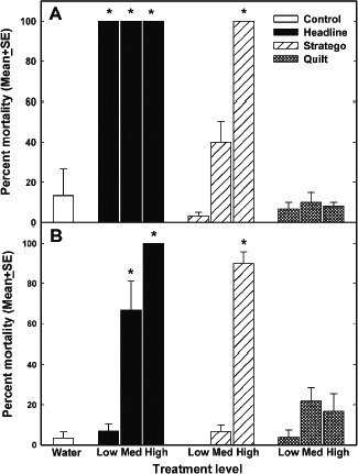
Mean percent mortality (± SE) of Bufo cognatus tadpoles (A) and juveniles (B) 72 h after a single exposure to either Headline, Stratego or Quilt fungicide at maximum label rate for corn (Med), or 0.10 label rate (Low) or 10x label rate (High). From Belden et al. (2010)
Significant levels of toxicity were noted for two out of three fungicides. All concentrations of the fungicide Headline resulted in 100% tadpole mortality and the medium and highest concentrations resulted in significant toxicity to juveniles (Figure 1).
Since mortality occurred mostly within the first 24 h after spraying, the authors concluded that ‘thus, juveniles exposed in a normal spraying event, such as in a field undergoing fungicide application, will likely not survive. Furthermore, tadpoles in a wetland directly sprayed or exposed to spray drift at 10% of the application rate will likely not survive’. The water concentrations in the low rate compared roughly to a calculated realistic worst‐case environment concentrations in surface waters not oversprayed and without further refinements (FOCUS step 1 at intended uses in Europe). The authors concluded further that comparative acute sensitivity was to be expected for fish and crustacean species, but that no similar comparison was possible for aerial exposure of juvenile toads. It was argued that behavioural patterns vary among species, but that the tested species is active during the day and spends much of its time above ground, potentially resulting in full exposure. Furthermore, potential exposure might vary with age, but newly morphed individuals of all amphibian species in the investigated area Great Plains are present above ground during daylight hours (Belden et al., 2010).
Brühl et al. (2013) mimicked exposure in a terrestrial environment where juvenile frogs were directly oversprayed by authorised field rates. The effects of seven PPPs (four fungicides, two herbicides and one insecticide) on juvenile European common frogs (Rana temporaria) were investigated. The selected PPPs are regularly employed in cereals and orchard in Central Europe (Germany and Switzerland). For one of the PPPs containing the active substance pyraclostrobin, a formulation of known toxicity was also tested (Headline EC, Belden et al., 2010) in addition to another type of formulation with the same active substance (BAS 500 18 F).
The tested rates for all PPP were those authorised for the intended uses (label rate 1x), a tenth of the label rate (0.1x) and ten times the recommended label rate (10x; see Figure 2). The test set up was again a realistic worst‐case scenario for terrestrial exposure of juvenile frogs leaving breeding ponds in spring. The frogs were exposed to PPP overspray in terrestrial microcosms with natural soils, and for the following seven days also to residues of the applied PPP in the soil matrix.
Figure 2.
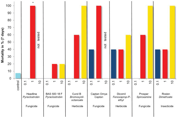
Mortality of juvenile European common frogs (Rana temporaria) after seven days following an overspray exposure for seven pesticides at 0.1×, 1× and 10× the label rate (formulation name, active substance and class are given). From Brühl et al. (2013)
As a result of the exposure, acute mortality ranged from 100% to 20% after seven days at the recommended label rate of currently authorised PPP intended uses (Figure 2). Some of the current authorised pesticides caused the observed 100% effect after 1 h of exposure (please see for details Brühl et al., 2015) Three PPPs out of seven caused a mortality of 40% after 7 days at the lowest rate tested (10% of the authorised rate). PPPs with the same active but varying in formulation type showed pronounced differences in acute toxicity for this amphibian species: one formulation caused 100% mortality after 1 h, while another formulation with the same concentration of active substance caused only 20% mortality in the rate corresponding to 10x the authorised rate. The relation between the juvenile frog mortality and some specific parameters (e.g. content of naphtha‐compounds as co‐formulants, log Pow of the active substance) as well as additional toxicity data (fish toxicity, inhalation toxicity, potential for eye irritation) was further investigated (Brühl et al., 2015). The calculations of simple linear regressions revealed no statistically significant relationship for the majority of the investigated parameters, which may be due to the low number of pesticides investigated. The only relationship that proved to be statistically significant was the one detected between values of product‐inhalation toxicity and the toxicity to R. temporaria. Furthermore, the inclusion of skin sensitisation as categorical variable increased the statistical significance of the correlation.
In the study set‐up of Brühl et al. (2013), it could not be determined whether the active substance itself or effects of co‐formulants determined the final toxicity of PPP for amphibian terrestrial stages. Further data submitted by notifiers to EFSA and national authorities for active substance and PPP authorisation confirm that the active substances can drive the toxicity of PPP and that the formulation type can modulate this toxicity (see Table 1). Overspray can be seen as a realistic worst‐case exposure scenario, whereby interception by plants might reduce the exposure of these animals in‐ and off‐field.
Table 1.
Toxicity of three PPPs with the same active ingredient but different formulation type expressed as toxicity to exposure ratio (TER) between the mean lethal rate (LC50) or rate causing no mortality (LC0) and the intended field‐application rate. The test organism was the amphibian Rana temporaria in a realistic worst‐case overspray scenario
| Formulation | Formulation type | TER [LR50 g a.s./ha/field rate g a.s./ha] | TER [LR0 g a.s./ha/field rate g a.s./ha] |
|---|---|---|---|
| A | EC | 0.38 | 0.25 |
| Blank formulation A | EC | >> 0.39 | ≥ 0.39 |
| B | CS | ~ 7 | ~ 2 |
| C | WG | > 2.04 | 0.92 |
a.s: active substance; EC: emulsifiable concentrate; CS: capsule suspension; WG: wettable granules. Adapted from information submitted for pesticide registration.
For the one active substance that was formulated in different products A, B and C, acute toxicity values for R. temporaria exposed in an overspray scenario differed by a factor 6–7 (see Table 1). Here, the formulation type also differed between the tested products, not only the composition of the co‐formulant system. Formulation B was a slow‐release capsule suspension and C water‐dispersible granules.
Interestingly, data are also available for the blank formulation without active ingredient of product A as an emulsifiable concentrate. The results of the tests with product A and its blank formulation show that the active substance itself is the driver of the product toxicity and not the co‐formulants, since no effect could be detected at the highest tested rate of the blank formulation, while at the same rate exposure to the product resulted in 70% mortality of the juvenile frogs.
The question arises why different PPP with different formulation types might have different effects if it is the active substance that causes the observed mortality. Apparently, the dynamic of the exposure of the organisms to the active substance is modulated by the type of formulation, most cleary seen in the lower toxicity of the slow‐release encapsulated formulation. Co‐formulants of the emulsifiable concentrate might possibly enhance the skin passage of the active substance without being toxic themselves (see Table 1). It appears that, for this active substance, the available amount over time and the dosage form determine its toxic effect via the dermal route for terrestrial stages of amphibians.
Contact with contaminated soil also delivers an important exposure path for frogs, although less crucial compared with overspray (see formulation A in Table 2). It should be noted, however, that no data with oversprayed Bufo bufo are available. If the PPP spray residues were allowed to dry up shortly before juvenile frogs were introduced, then the observed effects were higher than if animals were introduced after 4 h. Nevertheless, calculated toxicity to exposure ratio (TER) remained low also for this exposure route, showing a high toxicity of the formulation to juvenile frogs. Refinement steps are not presented at this stage, but would need to reduce exposure by a factor of approx. 2–40 in order to reach a TER of 10 on medial lethal acute mortality of juvenile amphibians.
Table 2.
Toxicity of a PPP in different test‐exposure scenarios, expressed as toxicity to exposure ratio (TER) between the mean lethal rate (LC50) or no observed effect rate (NOAER) and the intended field‐application rate. Test organism was the amphibian Bufo bufo placed on soil directly after spraying with the intended rate or several hours afterwards
| Formulation | Test set up | TER [LR50 g a.s./ha/field rate g a.s./ha] | TER [NOAER g a.s./ha/field rate g a.s./ha] |
|---|---|---|---|
| A | Animals introduced shortly after spray residue on soil dried up | > 1.2 | 0.6 |
| Animal introduced 4 h after spray application to soil | > 1.2 | ≥ 1.2 |
a.s: active substance; EC: emulsifiable concentrate. Adapted from information submitted for pesticide registration.
In conclusion, several of the tested PPPs show strong effect on the survival of amphibian terrestrial life stages at label rates or even less. The tested products and similar formulations (apart from Headline© for the US market) have been authorised for the market and have passed the assessment of the risks posed by their intended uses for all non‐target organism groups currently considered. Moreover, the concerns raised might even increase, considering that the exposure tested in all studies above is short‐term and mortality was the main endpoint assessed. Also, when taking into account possible exposure refinement (e.g. plant interception), risk might still be high, deeming for the time being a ratio between acute toxicity and predicted exposure (TER) of at least 10 as acceptable. As Belden et al. (2010) pointed out, ‘in an actual application, longer‐term exposure, chronic effects, and less tolerant species are all likely to occur’.
It has been shown (see Table 1) that the toxicity of the active substance itself can be the driver of the observed mortality for amphibian terrestrial life stages. Since the amount of available data is very poor, it cannot be concluded at the moment if – in cases where the formulated PPPs are toxic to amphibians – the active substance or the formulation would cause the observed toxicity. Interaction between toxicity of active substance, the co‐formulant system and the formulation type might interact in modifying the resulting impact on amphibians.
Assessment in the field
In assessing the relevance of laboratory findings for the population of amphibians in the wild, it has been recognised that the high sensitivity of amphibians to hormonal disruption, either through alteration of thyroid hormonal processes involved in development and metamorphosis or of estrogenic hormones involved in maturation and sex determination is one of the main aspects making amphibians different from other vertebrates in terms of toxicological susceptibility (Ortiz‐Santaliestra et al., 2017). Monitoring of endocrine and reproductive disruption in wild amphibian populations is hampered at present by a lack of validated biomarkers. Several field studies demonstrate increased incidences of gonadal intersex (the presence of ovarian follicles within the testicle) in male amphibians inhabiting agriculture intensive areas (Hayes et al., 2003; McCoy et al., 2008; McDaniel et al., 2008). Interestingly, male amphibians inhabiting habitats characterised by an increasing degree of agricultural activity displayed a gradual reduction in the display of secondary sex characters i.e. reduced forelimb size and nuptial pad size (McCoy et al., 2008). These findings may indicate an impact of antiandrogenic chemicals. Antiandrogens act by diminishing the action of androgens, either through androgen receptor antagonism or by changing steroid hormone metabolism. Several widely used pesticides (e.g. imidazoles) were recently shown to have antiandrogenic activity in vitro (Orton et al., 2011).
Laboratory studies have shown that environmentally relevant concentrations (0.1 or 2.5 μg/L) of the pesticide atrazine (not approved in Europe) can severely impair reproductive development and output in amphibians, i.e. Xenopus laevis and Lithobates pipiens (Hayes et al., 2002, 2003, 2010). However, in another study growth, larval development and sexual differentiation in developing X. laevis were not affected by 0.01–100 μg/L (Kloas et al., 2009). The apparently contradicting results were addressed in numerous papers (e.g. Solomon et al., 2008a,b; Hayes et al., 2011; Van Der Kraak et al., 2014).
In the work of Cusaac et al. (2015), field enclosures with cricket frogs (Acris blanchardi) were exposed in different settings in and around corn fields treated with the PPP Headline AMP. The amount of PPP reaching the soil was ~ 10% of the sprayed rates on top of the canopy and similar between field ground and spray‐drift areas outside the field. No statistically significant effects on survival of frogs could be detected in this experimental set‐up after 48 h, in which five fields containing three enclosure for each setting (spray, drift and reference) were averaged. These results could be expected from the laboratory data of Belden et al. (2010), where one‐tenth of the field rate resulted in mortalities ≤ 10%. Field tests are very challenging, and additional uncertainties have to be taken into account when evaluating the results (e.g. the statistical power of such studies and the occurrence of false negative results).
Davidson et al. (2001, 2002) reported a correlation on a larger scale between pesticide usage and amphibian decline in the Sierra Nevada Mountains in California owing to pesticide use on agricultural land upwind.
1.4.2. Reptiles
Direct evidence regarding protectiveness of the current risk assessment scheme on reptiles is missing, which is in part due to the scarcity of studies in this context. Rauschenberger et al. (2007) suggest that parental exposure to organochlorine pesticides (OCP) may be contributing to low clutch viability in wild alligators (Alligator mississippiensis) inhabiting OCP‐contaminated habitats in central Florida. Rodenticides as baits may be taken up when softened by rain by lizards and cause adverse effects (Spurr, 1993). Hall (1980) stated that reports of reptilian mortality from pesticide applications are numerous enough to establish the sensitivity of reptiles to these materials. Reports of residue analyses demonstrated the ability of reptiles to accumulate various contaminants, but the significance of the residues to reptilian populations remained unknown. Willemsen and Hailey (2001) provide a report of increased mortality to tortoises in areas sprayed with 2,4‐D and 2,4,5‐T in comparison to areas that were unsprayed. Finally, following a pesticide spill, Lambert (1997) found the reptiles avoided areas contaminated with at least 1 mg/kg pesticides in soil and lizards were absent when soil residue was above 10 mg/kg. Furthermore, one lizard from two species experimentally placed in contact with the soil causing dermal contact resulted in mortality of both individuals with 36 h.
Some field studies have assessed the responses of reptiles to pesticides focusing on physiological parameters. Sánchez et al. (1997) conducted a field test in order to evaluate the impacts of the application of a parathion‐based formulation (pesticidal active ingredient no longer approved for use in the EU) on giant Canary lizards (Gallotia galloti). These authors reported serum butyrylcholinesterase inhibition in lizards after field application of the insecticide, but did not assess any of the endpoints commonly used in pesticide risk assessment (e.g. mortality or reproduction). Amaral et al. (2012a,b) compared demographic, morphological, behavioural and biochemical parameters between Bocage's lizards (Podarcis bocagei) populations from northern Portugal inhabiting similar agricultural habitats that differed essentially in the use of pesticides (conventional vs. organic farming areas). They found that animals from conventional sites had poorer body condition, more internal parasites, higher levels of oxidative stress as indicated by the ratio between oxidised and reduced glutathione in the liver and, in a less‐than‐significant manner, a higher standard metabolic rate than lizards from organic sites. On the contrary, they did not find differences related to site in population size, individual biometry, ectoparasite prevalence, fluctuating asymmetry, hepatosomatic index, or liver and kidney histopathology. These studies were not designed to detect mortality or reproductive effects, but the obtained results, some of them analysing apical endpoints (i.e. body condition), demonstrate that lizards were exposed to pesticides in the field and that they can suffer adverse effects.
Recent data on cypermethrin in lizards (Chen et al., 2016) indicate that metabolic rates are strongly affected by external temperature and this may increase the elimination half‐life of pesticides (in this study, cypermethrin). Some reports on anticoagulants also show that these compounds are poorly metabolised by reptiles. The susceptibility of reptiles to anticoagulants is not known precisely but it appears that they may accumulate these compounds to a greater extent than other, more susceptible species such as mammals. Evidence from rodent‐eradication programmes in tropical islands confirms that reptiles (gecko) contained residues of brodifacoum in liver samples but did not display any evidence of poisoning (Pitt et al., 2015). Exposure experiments on Floreana lava lizards (Microlophus grayii), Geckos and snakes from the Galapagos archipelago were designed to reveal toxic effects on blood clotting. All animals were given brodifacoum‐poisoned prey over a 5‐day period and followed for three weeks. None of them displayed any evidence of abnormal coagulation (Fischer, 2011). Effects of pesticides used in corn and potato production in Canada on survivorship, growth and deformities of snapping turtle eggs (Chelydra serpentina) at male‐producing temperatures were investigated by De Solla et al. (2011). The herbicides atrazine, dimethenamid, and glyphosate, the pyrethroid insecticide tefluthrin, and the fertiliser ammonia, were applied to clean soil without historical contamination, both as partial mixtures within chemical classes, as well as complete mixtures at typical field application rates and higher (5.5 and 10 times field application rates) (De Solla et al., 2011). Egg mortality was 100% at 10× the typical field application rate of the complete mixture, which was later attributed to the fertiliser. At typical field application rates, hatching success ranged between 91.7% and 95.8% and was comparable to the control. Eggs exposed only to herbicides were not negatively affected at any application rates. The frequency of deformities of hatchlings was elevated at the highest application rate of the insecticide tefluthrin. The authors concluded that pesticides applied at the typical field application rates in corn production did not appear to have detrimental impacts upon egg turtle development of the snapping turtle at male‐producing temperatures using clean soil, but at higher rates the pyrethroid insecticide tefluthrin may increase deformity rates. A similar study was conducted with pesticides used in potato production (De Solla et al., 2014). The pesticide mixture consisting of chlorothalonil, S‐metolachlor, metribuzin and chlorpyrifos did not significantly affect survivorship, deformities, or body size at applications up to 10 times the typical field application rates, but the number of deformed turtles was higher in the treatments than in the control. Hatching success ranged between 87% and 100% for these treatments.
1.4.3. Conclusions and structure of the Opinion
Summarising the above, there is considerable evidence that active substances and authorised PPPs in Europe do have toxic impacts on amphibians and reptiles. Especially for the terrestrial life stages of amphibians, risk assessment based on effects on groups of non‐target organisms as currently assessed seem not to cover the risk of exposure to active substances or PPPs via the dermal route of exposure.
The PPR Panel therefore considers that initial suspicion is given for a thoughtful examination of actual risk assessment schemes, in order to provide the fundamentals for an operational assessment of active substances and PPPs. The PPR panel recommended already in the scientific opinion on the update of the data requirements (EFSA, 2007) that an appropriate risk‐assessment approach for amphibians should be developed. The aim is to ensure that those products are authorised that have no unacceptable effects on non‐target species, biodiversity and the ecosystem as required by current legislation (European Commission, 2009, Regulation (EC) 1107/2009).
The current opinion aims at providing the scientific basis for developing a future risk assessment scheme and covers the following topics:
Ecology and biology of amphibians and sources of environmental exposure, Section 2, p. 21
Definition of spatial aspects to be considered in the risk assessment, Section 3, p. 47
Population dynamics and modelling approach to support the setting of specific protection goals (SPG), Section 4, p. 50
Specific protection goal options for amphibians and reptiles, Section 5, p. 64 and Section 6, p. 68
General framework for developing a risk assessment scheme, Section 7, p. 78
Uncertainties in the risk assessment for amphibians and reptiles, Section 7.11, p. 95
Toxicological endpoints and standard tests relevant for amphibians and reptiles, Section 8, p. 103
Exposure assessment in the environment, Section 9, p. 122
Coverage of amphibians and reptiles by existing risk assessment schemes for other groups of organisms, Section 10, p. 137.
2. Ecology/biology of amphibians and reptiles and sources of environmental exposure to pesticides
Although amphibians and reptiles are studied together under the same branch of zoology (i.e. herpetology: animals that creep), they are very different animals with multiple biological and ecological characteristics extremely divergent between them. A description that defines these two groups in common is that they are poikilothermic tetrapods. Poikilothermy is the condition by which the internal temperature of an organism is subjected to wide fluctuations as a response of changes in environmental temperature. Poikilothermy is one of the most important aspects that make amphibians and reptiles different from other surrogate species like birds and mammals, which are homeothermic (i.e. their body temperature remains almost constant, regardless of environmental temperature).
2.1. Role of poikilothermy in environmental physiology and pollutant exposure
Poikilothermy determines many aspects of amphibian and reptile environmental physiology, and is a key factor in most of the characteristics that differentiate these animals from homeothermic tetrapods. These include metabolic rate, oxygen consumption and energetic expenditure, which in amphibians and reptiles are directly associated with fluctuations in environmental temperature (and therefore in body temperature) and play an important role in defining the potential toxic effects of an exposure to a chemical substance. Increased metabolic rates involve increased energetic demands and respiratory rates (Halsey and White, 2010), which can account for an increment of the chemical oral uptake or inhalation. For example, Avery (1971) described an increment of the daily food‐intake rate in green lizards (Lacerta viridis) during sunny days compared with partly cloudy ones. Moreover, animals tend to move more frequently as their metabolic activity increases, although this is not a fixed rule (e.g. basking reptiles have high metabolic activity but remain motionless). If animals move more frequently, the chances of chemical uptake grows. Although metabolic rate seems therefore associated with increased chances of chemical exposure, toxicants are more readily metabolised by more metabolically active organisms, which in turn reduces the risks of suffering toxic effects at the physiological level, as demonstrated by Talent (2005) with Anolis carolinensis exposed to pyrethrins. Toxicant metabolism, however, has an associated energy cost that can alter the relationship between metabolic and energetic investment in homeostasis, thus compromising other essential biological functions like growth, development, immunity or reproduction. As far as has been described, the mechanisms of pollutant metabolism and detoxification in amphibians and reptiles are not different from those of other vertebrates in terms of components (e.g. Katagi and Ose, 2014). The main determinant of the ability of these animals to transform and/or eliminate toxic substances from their bodies will be the rate at which metabolic processes work, which in turn depends on temperature. Therefore, poikilothermy constitutes a key issue, making chemical uptake, toxicokinetics and toxicodynamics in amphibians and reptiles somewhat different from what pertains in birds and mammals.
Homeothermic organisms spend most of the energy that they ingest as food in temperature regulation (Kronfeld‐Schor and Dayan, 2013). By contrast, poikilothermic animals, which use little or no energy to maintain body temperature, can invest most of the energy available from metabolism for other purposes such as growth. This major energetic investment in new body tissues determines some aspects of amphibian and reptile growth that have ecological importance. Poikilothermy allows growth rate to be adapted to the availability of resources in each territory and period of time, in such a way that growth is ratchet‐like rather than uniform (Andrews, 1982). This adaptability results in amphibians and reptiles being commonly present in habitats subjected to extreme environmental conditions, such as deserts (Mayhew, 1965), arctic regions (Costanzo et al., 2013), or water with salinity similar to that of seawater (Gordon et al., 1961).
Besides being adaptable to environmental conditions, growth in amphibians and reptiles is considered to be indeterminate, which means that organisms continue growing after sexual maturity. This is in contrast to species with determinate growth that stop growing once sexual maturity is reached (Seben, 1987). Indeterminate growth is also possible because of the great energetic investment in body tissues (Congdon et al., 2012), and is probably one of the reasons why amphibians and reptiles constitute an important part of the biomass in the ecosystems where they are present (e.g. Gibbons et al., 2006), sometimes in locations with low availability of resources. Growth is therefore a sensitive endpoint during the entire life of individuals. Nevertheless the relevance of potentially toxicity impaired growth will probably be higher during pre‐adult stages, when growth rate determines survival probabilities in later life (Semlitsch et al., 1988; Galán, 1996). In turn, amphibian and reptile communities are, because of the high biomass, important components of trophic nets; as consumers, they ingest large amounts of food, often with little specificity in the food choice, and consequently, play a role as sentinels of the nutrient composition of the ecosystems (e.g. Castilla et al., 1991; Luiselli et al., 2005). As prey, they constitute a major resource for top predators, and are therefore key elements in the transfer of energy and chemical substances across the food chains (e.g. Arribas et al., 2014).
In spite of all the similarities or common characteristics derived from poikilothermy that differentiate amphibians and reptiles from birds and mammals, both groups are so different that they require separate sections to explain most of the aspects of their general biology and ecology.
2.2. Main aspects of ecology and biology of amphibians
2.2.1. Origin and diversity
Amphibians include more than 7,000 known species (AmphibiaWeb 2016), with the highest species richness located in tropical regions. Living amphibians are grouped in three orders: anurans (toads and frogs, ~ 6,500 species), caudates (newts and salamanders, ~ 680 species) and caecilians (~ 200 species), the latter being absent from Europe. Amphibian diversity in the EU includes a total of 89 species (53 anurans and 36 caudates, Sillero et al., 2014), of which 23.6% (17% of anurans and 33% of caudates) are recognised by the International Union for the Conservation of Nature as endangered (i.e. listed within the categories of Critically Endangered, Endangered or Vulnerable for their global conservation status); this percentage can be locally higher if national or regional red lists are considered. In evolutionary terms, amphibians include the most ancient tetrapods, which appeared as fossils during the Devonian (360 million years ago), being the first vertebrates colonising the terrestrial environment (Duellman and Trueb, 1994). However, the fact that part of amphibian life cycle takes place in the aquatic environment makes amphibians not totally independent from the water.
The diversity of amphibians is patent in their body sizes and shapes. Anurans have a characteristic tailless morphology, with a robust body where head and trunk form a continuous unit and hindlimbs are usually much longer than the body, which is an adaptation to saltatory (hopping or leaping) locomotion. Not all anurans hop, however; some simply walk. Caudates have elongated, more or less cylindrical, bodies, thus with a higher surface area to volume ratio than anurans. They exhibit heads differentiated from the rest of the body, relatively long tails and short limbs, both hind and front pairs being of similar length.
2.2.2. Anatomy and function of skin
The dependence of amphibians on water is not only reflected in their life cycle. Amphibian anatomy, and in particular the characteristics of their integument, makes water balance a critical issue for these organisms. Amphibian skin lacks any kind of specialised structure of physical protection compared with other groups of terrestrial vertebrates, being very permeable to the diffusion of water and chemical agents. Therefore, skin is the main route of both water uptake and loss in amphibians. Chemical uptake of pollutants through amphibian skin has been suggested to be dependent on the octanol/water partition coefficient (log Kow) of each substance (Quaranta et al., 2009), although data obtained from live individuals indicated soil‐partition coefficient Koc was a better predictor than log Kow in determining bioconcentration factors of pesticides (Van Meter et al., 2014).
The anatomy of amphibian integument has been extensively studied (Barthalmus and Heatwole, 1994). The outer layer of amphibian skin is the epidermis, which is only a few cell layers thick (generally 2–3 cell layers in larvae and 5–7 in adults). In terrestrial stages, cells of the outer cell layer keratinise and die, forming the stratum corneum, which confers some sort of protection against excess water loss and injury. The innermost cell layer of the epidermis is called stratum germinativum and is continuously dividing to replace the outer layers. Thus, stratum corneum is periodically shed. During the yearly activity period, intermoult period can range from several days to few weeks, in a process mainly controlled by the hormonal system. The possibility that shed skin is used as a matrix for pollutant elimination in amphibians has not been explored. The moulting frequency does not seem to be species – but environment‐dependent. Paetow et al. (2012) observed that northern leopard frogs (Lithobates pipiens) individuals infected with Batrachochytrium dendrobatidis showed a higher moulting frequency than non‐infected ones, which could be interpreted as a mechanism to control pathogen loads; in the same study, frogs were also exposed to different levels of atrazine, which was found to have no effect on moulting frequency.
The dermis is behind the epidermis, separated from it by a thin basement membrane. The dermis is considerably thicker than the epidermis. The outermost region receives the name of stratum spongiosum and is formed by different structures, including glands, nerve ends, blood vessels or pigment cells, whereas the innermost part of the dermis, known as stratum compactum, is a tight net of connective tissue. The thickness and permeability of the skin vary from larval to post‐metamorphic stages but, even within adult forms, there are also some variations depending on whether they predominantly occupy aquatic, ground terrestrial or arboreal habitats as adults. These habitat‐dependent variations might influence dermal uptake of pollutants (Van Meter et al., 2014).
Tegumentary glands play important roles in amphibian relationships with the environment (Barthalmus and Heatwole, 1994); the abundant and evenly distributed mucous glands protect skin from desiccation. Holocrine glands are responsible for the secretion of antimicrobial substances, and granular glands secrete poisonous substances to repel predator attacks. These poison glands are often concentrated in the body parts most commonly targeted by predators, such as head and neck, and in many toad and salamander species can form macroglands on both sides behind the head known as paratoid glands. The internal mechanisms of activation of all these glands is not totally known, although the endocrine system is known to play an important role. Environmental stress affects glandular activity in the skin and can compromise the capabilities of organisms to keep skin moisture and water balance, or to defend them from pathogenic or predator attacks. Skin secretions could be another way of eliminating pollutants from the body in amphibians, though this possibility has not been investigated. If so, differential composition of glandular secretions could favour elimination of chemical substances with different physicochemical properties, but no research has been conducted in this context.
2.2.3. Water balance and gas exchange
In aquatic stages, water balance is generally not a problem; actually, permeability of amphibian skin to the water is up to 12 times higher in aquatic than in the terrestrial stages (Galey et al., 1987), which contributes to increased water diffusion, and therefore also to uptake of contaminants dissolved in the water. Terrestrial forms must, however, adopt mechanisms to avoid excessive water loss. On the one hand, several behavioural mechanisms like avoiding activity during high temperature or irradiation hours are common (e.g. Pough et al., 1983). In addition, amphibians show a so‐called water‐absorption response (Hillyard et al., 1998). The pelvic patch is an area of the posterior part of the ventral zone where skin is especially permeable to water because of its high degree of vascularisation. The water‐absorption response consists of pressing moist surfaces with the pelvic patch in such a way that a large volume of water can be absorbed in a short time. This results in potential for pesticide diffusion to be also higher through ventral than through dorsal skin (Kaufmann and Dohmen, 2016). On the other hand, the mostly granular skin of the dorsal and cephalic regions, which are the most exposed to air and solar irradiation, makes water permeability considerably lower than that of the pelvic patch. Some physiological adaptations also help terrestrial amphibians to maintain water balance, like the reduction of urinary water elimination by decreasing the rate of glomerular filtration and accumulating large volumes of water in the bladder (Geise and Linsenmair, 1986; Jørgensen, 1994). For this reason, mechanisms of osmoregulation, which are mostly controlled by hormones (McCormick and Bradshaw, 2006), are critical in maintaining water balance.
As mentioned above, metabolic rate in amphibians is strongly temperature‐dependent, with a more or less linear relationship between the metabolic rate and the body temperature (e.g. Whitford, 1973). Besides temperature, other factors like health or nutritional status, or the exposure to environmental pollutants, can affect metabolism as well (e.g. Ezemonye and Tongo, 2010). The metabolic demands under different situations are fulfilled in part thanks to the integrated involvement of the different respiratory organs (Shoemaker, 1992). Skin is an important respiratory organ in amphibians; in small individuals, where the surface area to volume ratio is high, skin breathing covers an important part of the necessities derived from the basal metabolism. In large animals, with a higher metabolic rate and a lower surface area to volume ratio, skin loses importance compared with lungs as the main organ of gas exchange. Some adaptations may, however, appear in large‐bodied animals to increase gas exchange through the skin, like increasing skin vascularisation or skin surface area by means of additional folds (Czopek, 1965).
2.2.4. Description of the reproductive system
Amphibian reproduction is characterised by a great variation with respect to breeding, fertilisation and embryo development. Most amphibian species have external fertilisation and embryo development, but embryo development inside the mother's body [ovoviviparity (inside egg) and viviparity] is observed in some species. Despite the variation in embryo development, the reproductive anatomy of the three amphibian orders (Anura, Caudata and Gymnophiona) shares the basic anatomical features. The male amphibian reproductive system consists of a pair of testes with adjacent fat bodies, a system of efferent ducts, Wolffian ducts (serving as ureters and sperm ducts), and the cloaca. The female amphibian reproductive system is composed of two ovaries with connected fat bodies, a pair of oviducts and a cloaca. There are, however, anatomical structures that are unique to certain species such as the Bidder's organ, which is present in the anuran family Bufonidae. The Bidder's organ is a structure that develops from the most anterior part of the gonads in both sexes. It resembles an ovary and contains immature oocytes but the function of this organ remains poorly understood (Ogielska, 2009). Another unique feature is the sperm‐storage glands called spermathecae localised in connection with the cloaca in females of most newt and salamander species (Ogielska, 2009). A third unique feature is observed in females of the viviparous caecilian Typhlonectes compressicauda, which have a specialised, placenta‐like structure in the oviduct (Ogielska, 2009).
2.2.4.1.
Gonadal sex differentiation
In most amphibians, the differentiation of the gonads into ovaries or testes starts during the larval period (Lofts, 1974). The process of gonadal development is similar in the three amphibian orders, but the majority of data originate from studies on anurans (Ogielska, 2009). There is, however, a great variation between amphibian species with regard to both timing and type of gonadal differentiation (Hayes, 1998). Variation occurs also within species, e.g. in the European common frog, R. temporaria, three types of gonadal differentiation pattern have been observed: differentiated, semi‐differentiated, and undifferentiated (Witschi, 1929). In the differentiated type of pattern, the gonads differentiate directly into ovaries and testes before metamorphosis. In the semi‐differentiated and undifferentiated types, the male gonads differentiate into ovaries before they transform into testes via an intersex stage. This transformation of the gonad occurs during metamorphosis in R. temporaria populations with the semi‐differentiated type and after metamorphosis, at the end of the first year, in populations with the undifferentiated type of gonadal differentiation (Witschi, 1929).
In the most common amphibian model, the African clawed frog (Xenopus laevis), the sexual differentiation of the gonads starts around Nieuwkoop‐Faber (NF) stage 56 (Tinsley and Kobel, 1996; see Section 8.1 for details on developmental stages), whereas in the western clawed frog (Xenopus tropicalis) the gonadal sex differentiation has been reported to start around NF stages 46–50 (El Jamil et al., 2008; Piprek and Kubiak, 2014). Before these stages, the gonads are sexually indifferent, i.e. there is no morphological difference between testes and ovaries. During ovarian differentiation, a cavity is formed in the centre of the gonad and the primordial germ cells are located in the surrounding cortex. In the male gonad, the germ cells are located in the medulla and no cavity is formed (Witschi, 1971). The ovarian cavity is therefore used as an early histological marker to discriminate between ovaries and testes.
Little is known about the mechanisms for sex differentiation in amphibians. All amphibians have genetic sex determination, the heterogamety appearing either in males (XY system) or females (ZW systems) depending on the species (Witschi, 1971). The sex differentiation of the gonads is, however, a plastic process compared with higher vertebrates. Experiments in anurans show that hormone exposure can override the genetic mechanisms and induce phenotypic sex reversal resulting in a skewed sex ratio compared with the control group (reviewed in Hayes, 1998). For instance, exposure to exogenous androgens, oestrogens or progestogens during critical periods of larval development causes complete or partial sex‐reversal of the gonads (Hayes, 1998). Cytochrome P45019 (cyp19, aromatase) mediates biotransformation of androgens into oestrogens. As sex hormones are important for gonadal differentiation in amphibians, this enzyme is supposed to have a role in sex determination. Aromatase is thought to be involved in gonadal differentiation in lower vertebrates as inhibition of aromatase in embryos of birds, reptiles and fish induces testicular differentiation (Elbrecht and Smith, 1992; Piferrer et al., 1994;. Pieau et al., 1999). The prevailing hypothesis is that aromatase is involved in amphibian gonadal differentiation but its specific role remains to be elucidated (Kelley, 1996; Urbatzka et al., 2007; Jansson et al., 2016). As explained below, temperature is an environmental factor that regulates gonadal sex differentiation in reptiles. In amphibians (anurans and caudates), experiments have shown that extreme (close to lethal) temperatures can influence gonadal sex differentiation (Hayes, 1998), but this does not seem to be a relevant factor for natural sex determination.
Müllerian and Wolffian duct development
The Müllerian ducts are present in both sexes in early life stages of amphibians, reptiles, birds and mammals, whereas they are lacking in teleost fish. In females, these ducts develop into the reproductive tract (i.e. the oviduct in amphibians, reptiles and birds, and the oviduct, uterus, and vagina in mammals). In males, the Müllerian ducts usually regress during early life stages. However, in males of Gymnophiona, the Müllerian ducts do not degenerate but instead develop into glandular organs (Ogielska, 2009). The growth and differentiation of the Müllerian ducts are under the control of hormones including oestrogens and progesterone. While it has been shown that gonadal differentiation starts during the larval stages in many amphibian species, there is little information on the ontogenetic development of the Müllerian ducts in amphibians. In Xenopus, the Müllerian ducts begin to form shortly before metamorphosis around NF stage 64 (X. laevis: Witschi, 1971; X. tropicalis: Jansson et al., 2016). The differentiation of the ducts into oviducts occurs in parallel to an increment of plasma levels of ovarian hormones. The oviducts are involved in egg formation in amphibians and are therefore crucial to their reproductive success.
The Wolffian ducts extend from the kidney to the cloaca and serve both as ureter and sperm duct in male amphibians. Enlarged regions of the Wolffian ducts serve as sperm‐storage sites close to the cloaca (Ogielska, 2009).
Oogenesis
Oogenesis is the process by which female germ cells undergo meiosis and differentiation into mature oocytes. The germ cells differentiate into oogonia, which proliferate before they enter meiosis. They are referred to as immature or primary oocytes as they enter the prophase of the first meiosis. The oocytes are then arrested in meiotic prophase during the whole process of folliculogenesis until gonadotropin‐induced signals trigger them to resume meiosis prior to ovulation (reviewed in Hammes, 2004). In most mammals, the early germ‐cell differentiation into primary oocytes is restricted to fetal life. In contrast, amphibians have a continuous oogenesis with germ cells differentiating into oocytes throughout life (Al‐Mukhtar and Webb, 1971). When the immature oocyte progresses beyond the early diplotene stage of meiotic prophase and becomes surrounded by follicular cells, it is referred to as a follicular oocyte. During folliculogenesis, the amphibian oocyte increases in size due to incorporation of the yolk precursor protein vitellogenin. Oogenesis is regulated by endocrine and paracrine control mechanisms involving steroid synthesis by the follicular and theca cells as well as the oocyte itself, reviewed by (Konduktorova and Luchinskaia, 2013).
Spermatogenesis
The frog testis consists of seminiferous tubules with germ‐cell nests in different maturation stages. The germ cells develop synchronously within each nest. The nests are produced when a Sertoli cell connects to a primary spermatogonium. The spermatogonium enters mitosis and produces a cluster of secondary spermatogonia enclosed by the Sertoli cell (Pudney, 1995). Secondary spermatogonia transform into primary spermatocytes that undergo meiotic division into secondary spermatocytes. Transformation then proceeds into round and elongated spermatids and finally to spermatozoa. The last step in spermatogenesis is spermiation, i.e. when the nest wall is ruptured and spermatozoa move into the lumen of the seminiferous tubule (Pudney, 1995). The process of spermatogenesis is complex and depends on endocrine and local controlling mechanisms that are not yet fully understood (Pierantoni et al., 2002; Sasso‐Cerri et al., 2004).
Bidder's organ
Bidder's organ is a structure that develops from the most anterior part of the gonads in anurans belonging to the family Bufonidae. Bidder's organ resembles an ovary and contains immature oocytes. The function of this organ remains poorly understood (Ogielska, 2009).
The larynx and sound production calling
Communication by sound production occurs in all three amphibian orders. The vocalisation system (including larynx and associated structures) and calling behaviour have been well characterised in several anuran species including X. laevis (Duellman and Trueb, 1994) and some European native species (e.g. Eichelberg and Schneider, 1974 for Hyla arborea). While the overall structure of the respiratory tract is similar between terrestrial species and aquatic species such as Xenopus, the larynx of the latter is specialised to produce sound underwater (Kelley, 1996).
2.2.5. Life history and reproduction
The common reproductive strategy involves an aquatic egg in which the embryo develops to a larval form, also aquatic. At the end of the larval stage, individuals undergo a metamorphosis process during which they transform into a terrestrial juvenile, morphologically and anatomically similar to the adult form (Figure 3). In temperate and cold‐temperate regions, the amphibian breeding cycle is strongly seasonal. In most of EU territory, the breeding season begins at some point in spring, shortly after animals emerge from overwintering. Aquatic stages then develop during most of the spring and summer to emerge as terrestrial forms in summer or autumn, before the temperatures drop again. There are, however, many exceptions to this general scheme; some species, or certain populations of some species, do not lay eggs but are either viviparous or ovoviviparous, giving birth to more or less developed larvae (Wake, 1993). Some populations have larvae that hibernate and do not emerge until the next spring (e.g. Gilbert and ter Harmsel, 2016) or, in areas with mild winters and extreme temperatures in summer (which in Europe would correspond to the southernmost areas of the Mediterranean basin), an aestivation period followed by an autumnal or winter breeding season (e.g. Gomez‐Rodriguez et al., 2012). The seasonality of the life cycle of amphibians results in the presence of periods during which animals rely on accumulated reserves. These periods are critical from a toxicological perspective, as accumulated pollutants could also be mobilised as part of the consumption of internal reserves (James et al., 2004), as has been described in fish and homeothermic vertebrates (Daley et al., 2014). Especially long resting periods could take the availability of internal reserves to the limit, resulting in animals awaking in a very impoverished condition, but also with a high potential of having mobilised significant amounts of accumulated pollutants.
Figure 3.
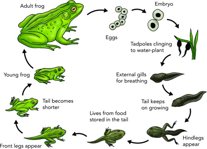
Representation of the life cycle of a frog exhibiting the amphibian common reproductive mode (taken from Siyavula Education. Image under License Creative Commons Attribution 2.0 Generic. Retrieved on 29 November 2016) from website at https://www.flickr.com/photos/121935927@N06/13578724373
At the beginning of the breeding season, adults generally migrate from their refuges to water bodies (see Habitat and movements section below) where eggs are laid. Amphibians generally use courtships to attract mates; this strategy ensures that both male and female gametes have achieved the maturation stage and are ready for fertilisation, as well as placing both gametes in close proximity before gamete transfer and eventual fertilisation (Vitt and Caldwell, 2014). Fertilisation is external in most anuran species and in a few caudate groups (reviewed in detail in Duellman and Trueb, 1994); the male sheds the sperm on the eggs as they are being released through the female's cloaca. In anurans, the male grabs the female in a posture known as amplexus; the part of the body where males grab the female varies among species, resulting in different types of amplexa (e.g. inguinal, axillar, cephalic). In caudates with external fertilisation, male and female cloacae are normally close at the end of the courtship and sperm is deposited on top of the egg mass during or right after release. Most caudates, as well as caecilians and a few frog species have internal fertilisation, either by cloacal contact (some frogs), male intromitting organs (some frogs and all caecilians) or through a spermatophore that is picked up by the females (caudates). In caudates with internal fertilisation, females may storage sperm for long times (up to several years); this is supposed to allow females to select the time of fertilisation and further egg laying in order to optimise embryonic development conditions.
Amphibian eggs are encased in an envelope formed by several layers of mucoprotein and mucopolysaccharide (Viarengo and Falcone, 1977). The envelope, upon release and contact with the medium water, acquires a gelatinous texture that contributes to protect eggs from mechanical damage and from other threats like predation, ultraviolet radiation and uptake of some environmental chemicals (Ward and Sexton, 1981; Marquis et al., 2006). Some species provide additional parental care to their eggs by carrying them on their backs or rear legs (e.g. genus Alytes) or even inside a dorsal skin pocket (e.g. genus Pipa), wrapping them with aquatic plant as in many newt species, or making foam nests inside which not only embryos but also larvae can develop (observed in leptodactylid species) (Duellman and Trueb, 1994). Maternal deposition of pollutants to the eggs is known to exist in amphibians, although the patterns influencing this process have not been investigated in depth. Metals, trace elements and persistent organic pollutants can be transferred from maternal bodies to the eggs (e.g. Kadokami et al., 2004; Metts et al., 2013), which can sometimes result in reduced offspring viability (Metts et al., 2013). Maternal deposition of pollutants into the eggs could be a way of detoxification (Kadokami et al., 2004), preserving maternal organisms at the expense of offspring; at the population level, this could be beneficial in those species relying more on adult survival than offspring survival, which is typical of so‐called r‐strategists (see Annex A for how to assess such effects using sensitivity or elasticity analysis).
Although most amphibians have very large clutch sizes, this parameter size may vary among species within an extremely wide range from a few tens to several thousands of eggs per female. Following a general rule in the animal kingdom, species that use more energy in producing large amounts of ova put less energy into ensuring offspring survival; this is the case in many toads that may lay several thousands of eggs per female. At the other end of the life‐history continuum, those species showing parental care are the ones with smaller clutch sizes; for example, females of midwife toads of the genus Alytes lay only a few tens of eggs per year, but these eggs are then carried by adult males until hatching, which can contribute to reduce embryonic mortality.
Larvae possess hatching glands that secrete proteolytic enzymes, which degrade the gelatinous capsules to facilitate their breakage (Nokhbatolfoghahai and Downie, 2007). Hatching in amphibians normally occurs early in embryogenesis, such that most of the aquatic development is accomplished by a free‐living larva. There are, however, some species with direct development in which hatching happens at the end of development, and what emerges from the egg is not a larva but a fully formed juvenile morphologically similar to the adult. In these species, there is no real metamorphic event (Duellman and Trueb, 1994).
Larvae of most amphibian species are aquatic, with a very thin skin consisting of only two or three epidermal layers, highly vascularised to facilitate its role as a gaseous exchange organ. The skin is not the only respiratory surface in amphibian larvae; this function is shared with the gills, which are normally external during the initial stages of larval development (McDiarmid and Altig, 2000). Caudate and caecilian larvae retain external gills throughout the entire larval period, but in most anurans, gills become covered by the operculum as development progresses. In these species, one or two spiracles remain open in the operculum to allow the flux of water. The location of the spiracle(s) varies among species. The presence of external gills during part or all the larval development has the function of providing increased surface area for gas exchange; such an increase of the surface area to volume ratio can also lead to an increased rate of chemical absorption in the water. That is the reason why newly hatched individuals are commonly identified as the most sensitive ones among amphibian aquatic stages (Ortiz‐Santaliestra et al., 2017).
Larvae of caudates and caecilians are morphologically similar to adults. In caudates, the four limbs are developed at the very beginning of the development. In contrast, anuran tadpoles are very different from adult forms. Their main functions are feeding and growth, for which they present large coiled intestines and specialised oral apparatus consisting of a disc with several rows of keratinised labial teeth and sometimes jaw sheaths, everything covered with papillae (Altig, 2007). Morphological variations exist across tadpoles on the basis of their diet, foraging strategy and type of habitat. Limbs in anuran tadpoles are developed at the end of the larval period; hindlimbs are the first to emerge, whereas forelimbs, although developed at the same time as hindlimbs, remain covered by the operculum and do not emerge until metamorphosis (Duellman and Trueb, 1994).
The duration of embryonic and larval development also varies across species, although it is strongly determined by environmental conditions. Amphibians show a phenotypic plasticity that allows for adjusting developmental pace to the conditions of the environment (e.g. Richter‐Boix et al., 2006). This plasticity results, for example, in accelerated larval development with increased temperatures, which could allow for larvae to complete development and metamorphosis before ponds desiccate. Several studies have postulated the negative impact that pollutant‐related alterations of developmental rates could exert on this phenotypic plasticity, and consequently on the ability of amphibian larvae to respond to changing environmental conditions (e.g. Burraco et al., 2014). In experimental conditions, there are many studies demonstrating that exposure to environmental pollutants decelerates developmental rate. Besides the impact that this effect may have on phenotypic plasticity, a longer time to complete development also tends to involve a prolonged exposure to the pollutants in the aquatic environment, which results in a positive feedback potentially enhancing negative effects of pollution on embryonic and larval development. Overall, duration of larval development can range from less than 20 days to several years. This plasticity in larval development can result in larvae of a given species reaching metamorphosis, not only at different times, but also with variable sizes. As long as the conditions in the water remain good (e.g. enough food and no desiccation, predation or infection risks), larvae can continue growing to reach metamorphosis with a larger body size, which is generally associated with increased juvenile success (e.g. Cabrera‐Guzmán et al., 2013). In polluted environments, however, the amount of energy spent in toxicant metabolism cannot be allocated to growth, which results in reduced growth rates and loss, at least partially, of the theoretical advantage of prolonging larval life to metamorphose with a larger body size.
The larval period finishes with the metamorphosis. Metamorphosis is a key process in the life history of amphibians in which larvae transform into juvenile, adult‐shaped forms. The morphological and anatomical reorganisation is especially intense in anurans. Metamorphosis involves not only morphological changes, but also a series of physiological modifications of almost all systems necessary to transform an aquatic organism into a terrestrial one (Gilbert and Frieden, 1981). Metamorphosis is mostly regulated by thyroid hormones (Kikuyama et al., 1993), with all the processes happening during metamorphosis resulting from differential exposure of the involved tissues to the thyroxine hormone (TH). Some other hormones like corticosterone and prolactin also play a role in regulation, acting as inhibitors during larval life and disappearing towards the end of the larval period to allow TH to initiate the process of metamorphosis (Etkin and Gona, 1967). The action of TH release is in part responsible for the developmental plasticity of amphibians. Several environmental factors can promote the release of TH, thus affecting the timing of beginning of metamorphosis and consequent emergence of the individual from its aquatic habitat. Like overwintering or aestivating periods, metamorphosis is toxicologically critical because of the potential mobilisation of reserves, and therefore of pollutants, accumulated during the larval period (Sparling et al., 2006a). Metamorphosing individuals do not eat but, in contrast with what happens during resting periods, maintain a high activity and metabolic rate, which results in a quick consumption of the body reserves. The proportional body mass loss during metamorphosis could be a direct indicator of the risk of suffering toxic effects because of mobilisation of accumulated substances.
Age at sexual maturity varies from a few months, especially in tropical species, to up to seven years in large salamanders (Vitt and Caldwell, 2014). In general, the age at sexual maturity is subjected to a trade‐off between early maturation (which relates to reduced offspring size and increased chances of predation of adults) and breeding and maturing at a larger size (which results in increased pre‐adult mortality and reduced number of reproductive events throughout the entire lifespan), although this can be modulated by the fact that size at sexual maturity does not necessarily correlate with age but also with juvenile growth rate (Halliday and Verrell, 1988). In addition, maximum lifespan is generally correlated with age at sexual maturity in such a way that individuals attaining the reproductive status during the first or second year of life rarely live more than five years, whereas those animals reaching sexual maturity at older ages can live up to 25 years (Vitt and Caldwell, 2014).
2.2.6. Habitat and movements
Amphibians are widely distributed across the Earth, being present on all continents but the Antarctic and occupying a great variety of habitats if water bodies are available for breeding. Over the last 25 years, evidence has grown pointing to a global decline of amphibian populations: the main reasons, according to the Global Amphibian Assessment, are habitat loss and environmental pollution (IUCN, 2008). In agricultural areas, where these two factors co‐occur, the presence of amphibians is well known, and in Europe, up to 38 amphibian species (43% of the amphibian diversity) are identified by the International Union for the Conservation of Nature (IUCN) as inhabiting arable lands. Although the majority of amphibian populations inhabiting agroecosystem seem to prefer off‐field sites (e.g. Miaud and Sanuy, 2005; Oromi et al., 2010), the occupation of arable areas can occasionally be dominant, as observed by Cooke (1986) with adult great crested newts (Triturus cristatus) preferring mature wheat fields to marsh or woodlands. In other cases, the use of arable fields is restricted to particular activities like feeding (Oldham and Swan, 1992) or moving (see below).
The spatial ecology and habitat selection of amphibians are very important in determining the chances of exposure of their terrestrial stages to environmental pollution, especially in agricultural areas. Home ranges in amphibians are generally small, and a particularity of amphibian spatial ecology is that, in many species, home ranges change with the season. For most European species, animals tend to concentrate around water bodies during breeding seasons, whereas the rest of the activity period they occupy terrestrial environments where they search for food. Terrestrial feeding habitats may also coincide with resting areas during inactive periods (Indermaur et al., 2009). This creates a very variable spatial pattern of chemical exposure, as seasonal movements may result in animals travelling across areas with potentially different degrees of contamination (Regosin et al., 2005). Another peculiarity of amphibian spatial behaviour is the high degree of site fidelity, especially in what refers to breeding habitats. Year‐to‐year faithfulness to breeding sites has been reported as 88–98% in wood frogs (Lithobates sylvaticus), 79–96% in common toads (Bufo bufo) and up to 100% in spotted salamanders (Ambystoma maculatum) (Reading et al., 1991; Vasconcelos and Calhoun, 2004). In the event of a continuous or repeated occurrence of pollutant in the habitat, this pattern will presumably have a major influence on the exposure of breeding adults, as well as of aquatic stages, to contaminants, not only because of repeated exposures over time but also because it will restrict the capacity of searching for alternative, unpolluted sites.
Amphibian breeding migrations from wintering sites to breeding points, together with the return trip at the end of the season, and emergence and dispersal of juveniles after metamorphosis constitute the most typical movement events in amphibians. Breeding migrations are directional and have clearly defined destinations. Migrations can run over the shortest distance to the target point without or with little selection of the habitat to cross on the way (e.g. Pilliod et al., 2002), which increases chances of crossing less suitable habitats; alternatively, migrations can run through more suitable corridors (Hartel and Demeter, 2005), reducing chances of travelling across less suitable habitats. Dispersal movements, on the contrary, are usually not predefined, although they tend to orientate non‐randomly towards the most suitable habitat patches (Vasconcelos and Calhoun, 2004). Besides these aspects, a particularity of both types of movements is that they occur massively, with an important proportion of the adult or juvenile populations moving at the same time. In terms of risks from pollution, if there is spatial and temporal overlap of sources of pollution and presence of amphibians, these phases of the life cycle are critical because of the important effects that could occur at the population level. Amphibian‐breeding migrations may happen over short distances (e.g. few hundred metres as generally seen in newts; Schabetsberger et al., 2004) or they can be rather long (e.g. > 4 km for Epidalea calamita; Miaud et al., 2000). Equally, post‐emergence, dispersal movements can also go over 1.5 km (Sinsch, 1988).
Some amphibians are known to cross crop fields in spring, while migrating towards breeding ponds (Miaud et al., 2000; Miaud and Sanuy, 2005; Kovar et al., 2009; Lenhardt et al., 2013), temporally and spatially overlapping with periods of pesticide application (Berger et al., 2012, 2013; Lenhardt et al., 2015). The risk of coincidence with pesticide application is nevertheless very variable; the percentage of amphibian populations moving over agricultural sites coinciding with pesticide application could vary from 20% to almost 90%, depending on the species, crop types and years, according to Berger et al. (2011). Amphibian‐breeding migrations can be facilitated if animals use arable lands. At the beginning of the activity period, when animals migrate towards the breeding sites, vegetation cover in crop fields is very low, which favours easy and quick displacement of animals. Berger et al. (2011) observed use of recently ploughed fields for dispersal of some species including the common toad (Bufo bufo), although during daytime resting periods, animals tended to look for refuge in densely vegetated areas. Individuals of other species like the spadefoot toad (Pelobates fuscus); however, dug themselves to find shelter, and loose, ploughed fields facilitate this strategy. Individuals may therefore stay inside crop fields for entire days during their breeding migrations. In other cases, migrating toads have been observed to move along pasture corridors, avoiding arable lands (Hartel and Demeter, 2005). Crossing arable fields during breeding migrations seems therefore to be dependent on habitat structure, temporal variations in the vegetation cover and other characteristics of different habitat patches, and particular preferences of each species or population.
2.2.7. Feeding ecology
Adult amphibians, as well as caudate larvae, are mostly carnivorous and feed generally on small arthropods. The type of preferred prey is normally related to the body size of the animal (e.g. Labanick, 1976), in such a way that the net energy obtained in each feeding event is optimised as a function of the prey size (related to gross energy income) and the effort necessary to capture and manipulate it (energy spent in the activity itself). This leads to inconsistencies between the preferred prey if they are considered either in terms of number of ingested items or in terms of ingested biomass. In general, amphibian diet is opportunistic (Duellman and Trueb, 1994; but see Simon and Toft, 1991), and the diet composition seems to respond to the type of prey available within the optimal prey sizes in each case. Newt and salamander larvae feed mostly on zooplankton. Anuran larvae, on the contrary, are omnivorous and feed mainly on periphyton, grazing on sediments, although other feeding modes like filtering phytoplankton or skimming the scum at the water surface are also very common among anuran tadpoles (McDiarmid and Altig, 2000; Altig et al., 2007).
Feeding behaviour, like diet composition is highly variable. Among carnivorous forms, aquatic‐feeding individuals are generally active predators, whereas terrestrial individuals may show either active search or ambush (i.e. ‘sit‐and‐wait’) strategies. Because of the differences in energy expenditure between the ambush and active modes, active foragers should tend to compensate the greater energy loss through a less specific diet (Schoener, 1971).
Estimating food‐intake rate in amphibians is complicated. The amount of ingested food as well as the time spent feeding fluctuates daily (Larsen, 1992), which is probably a consequence of the environmental dependence of physiological activity and therefore of nutrient necessities, associated with poikilothermy. Larsen (1992) estimated a yearly uptake of 142.4 kJ for a male common toad weighing 30 g. Estimating a daily food‐intake rate from this value is, however, difficult because of the aforementioned fluctuations among days, even within a given activity period. Assimilation efficiency is a key factor, not only to infer food‐intake rate, but also to estimate the likelihood of ingested pollutants being absorbed in the intestine. The data show how energy gain is a function of the type of prey ingested, with mealworms appearing as the most profitable prey (assimilation efficiency > 90%; Dimmitt and Ruibal, 1980), followed by flies (79–91%; Bobka et al., 1981; Grafe et al., 1992), crickets (73.7%; Smith, 1976), and beetles (65–66%; Dimmitt and Ruibal, 1980). The majority of these studies on nutritional physiology coincide in pointing an inverse relationship between temperature and gut retention time, which results in the expected higher assimilation efficiency at lower temperatures (but see Smith, 1976). Higher assimilation efficiency at lower temperatures allows amphibians to reduce the number of feeding events, which is consistent with their reduced activity, movement and metabolism as temperatures drop.
2.3. Main aspects of ecology and biology of reptiles
2.3.1. Origin and diversity
Although amphibians constitute the initial evolutionary step of the colonisation of terrestrial environment by tetrapods, they were unable to become independent from the water as most of them need the aquatic environment to complete their life cycle. The early amniotes, ancestral to all reptiles, became able to reproduce in the absence of water and developed a skin protection against evaporative water loss, completing the process of land colonisation initiated by the ancestor of amphibians. These forms appear as fossils during the Carboniferous (320 million years ago) and gave rise to the different lineages resulting not only in all past and present forms of reptiles, but also of birds and mammals (Carroll, 1969).
Extant reptiles belong to three major clades: archosaurians, which include crocodilians as well as birds, testudines (turtles) and lepidosaurians (squamates and tuataras). Crocodilians, with 25 living species, and tuataras (a single species) are not present in Europe. Testudines comprise 346 extant species (seven of them in the European Union, excluding the Macaronesia, northern African sites, and overseas territories; Sillero et al., 2014), whereas living squamates are divided into three suborders: amphisbaenians or blind snakes (196 species, two in the EU), saurians, including lizards, skinks, geckos, iguanas, etc. (6,263 species, 76 in the EU), and ophidians or snakes (3,619 species, 35 in the EU). Turtles have bodies typically covered by a shell formed from the fusion of the tegument and the thoracic skeleton, with a lower (plastron) and upper (carapace) parts that normally fit together. Within this general uniformity of shapes, turtles have a wide ecological range, from marine to fully terrestrial species (tortoises), including forms associated with freshwater environments (terrapins). Body shapes and sizes in squamates are much more diverse than in any other reptile group, from very tiny geckos to large snakes, from limbless forms to animals with robust legs, like iguanas, and from species living in deserts to semiaquatic or arboreal forms. In parallel with this morphological variability, surface area to volume ratios are very different among species (e.g. long, slim snakes will have higher surface area to volume ratios than large lizards or chameleons with more compressed shapes). Interestingly, some reptile groups do not seem to follow Bergmann's rule that predicts larger body sizes (and therefore reduced surface area to volume ratios) in species living in colder climates (Bergmann, 1847). The particular necessities of reptiles with regard to heat gain (see Thermoregulation and gas exchange section below) cause this trend to be reversed in lizards and snakes (Ashton and Feldman, 2003), which leads to species in temperate areas (more favourable for agriculture) tending to show lower surface area to volume ratios than species in cold areas.
2.3.2. Anatomy and function of skin
Although the skin of reptiles is structurally similar to that of amphibians, several important differences can be found (Lillywhite and Maderson, 1982). The reptilian epidermis has a higher number of cell layers than in amphibians, which results in a thicker section of keratinised cells. Furthermore, reptiles are unique in producing β‐keratin, which is hard and brittle and combines with the more elastic and pliable α‐keratin typical also of other vertebrates. The skin in reptiles is usually modified in scales, which share the characteristic of being keratinised epidermal parts, but have different structures and names depending on the taxonomic group and the body region. Scale surfaces are formed by β‐keratin, whereas sutures of separation between scales are formed by α‐keratin. Epidermal growth patterns are also variable among groups; in lepidosaurians, the stratum germinatum divides in a cyclic manner, in such a way that two epithelial layers are superposed in the outermost part of the integument. In crocodiles and turtles, skin growth is continuous, only with the corresponding periods of arrest during hibernation or aestivation. This variation in epidermal growth patterns also results in differences in the process of skin shedding or ecdysis. Thus, whereas in lepidosaurians skin is shed all at once or in large patches, with a very uniform periodicity (interrupted however by a variable resting phase in the process of cell differentiation), in crocodiles and turtles, small flakes of the skin are continuously being shed (Irish et al., 1988; Maderson et al., 1998). Shed skin from some snakes has been analysed for pollutant presence in order to estimate whether this could be a way of toxicant elimination, finding detectable levels of metals and POPs (Jones et al., 2005; Jones and Holladay, 2006). It is difficult, however, to establish how important skin shedding might be as a detoxification mechanism in reptiles without a more detailed monitoring of internal concentrations in animals.
The dermis of some reptilian species has osteoderms, bony plates that underlay scales and are disposed in layers, with an outer, spongy layer formed by porous bone and an inner, compact layer formed by dense bone tissue (Lillywhite and Maderson, 1982). In most cases, osteoderms are simply attached among them forming an additional protective layer; in some cases, they can fuse with pieces of the skeleton, like vertebrae, ribs and sternum in turtles, to form rigid shells (Hirasawa et al., 2013). The presence of glands in reptilian skin is common, although in a lower number and diversity of forms than in amphibians. The major roles of these glands are for the secretion of pheromones and impermeable waxes (Quay, 1972).
Because of these highly keratinised structures, reptilian skin is commonly viewed as a barrier against dermal uptake of contaminants (Snodgrass et al., 2008). Weir et al. (2010), however, pointed out that permeability of the skin to pollutants would be more likely affected by lipid content than by keratin content of the skin. Reptile skin normally has a high lipid content (Pough et al., 2004), which will prevent diffusion of hydrophilic contaminants but allow absorption of lipophilic ones.
2.3.3. Thermoregulation and gas exchange
Metabolic rate in reptiles is temperature dependent, as in amphibians. There is, however, decoupling, in some lizards and snakes, between both parameters over the range of preferred temperatures, in such a way that metabolic rate keeps invariant across a window of 3–5°C (Bartholomew, 1982). A notable difference from amphibians in this context is the relative importance of skin as a respiratory organ, which in reptiles is really low, the vast majority of gas exchange being done through lungs.
Thermoregulation is the process by which the organism exchanges heat with the environment, and is a key factor to all physiological functions. Thermoregulation may have the function of warming up or cooling down the body, depending on the environmental conditions. Evaporative water loss through the skin of amphibians must be minimised; therefore, activity at higher temperatures is normally lower than in reptiles (Tracy and Christian, 2005), for which water loss through the skin is generally not an issue. Critical thermoregulation in amphibians is generally focused on cooling down during warm periods, whereas gaining heat is usually the function of thermoregulation in reptiles. Reptiles are usually active during sunny, warm days and, within these, during the hours when temperatures are close to their optimal. This means that, in temperate areas, daily activities in spring and autumn are normally unimodal (with a single active period in the central part of the day) whereas activity in summer is bimodal (with two active periods in the morning and late afternoon, avoiding the very high temperatures of the central part of the day). This pattern is of course subjected to variations depending on the environmental conditions of each specific location. Heat gain is achieved through two mechanisms: heliothermy consists of gaining heat by basking in sun, and thigmothermy consists of gaining heat by conduction from warm surfaces not necessarily exposed to the sunlight. Although most species have relatively broad ranges of temperature of activity, the preferred temperature range is narrow, and the closer that animals are to this temperature, the better their physiological functions work (reviewed by Seebacher and Franklin, 2005).
2.3.4. Life history and reproduction
Reproductive modes in reptiles can be broadly divided into two major groups: oviparity and viviparity. The former is the most common mode in the group, including all crocodilians, turtles, tuataras and most squamates. Viviparity occurs in approximately 20% of squamates (Vitt and Caldwell, 2014). Viviparity in reptiles appears as an adaptation to cold climates, with short periods of appropriate conditions for activity and development of offspring. The timing of the life cycle of European reptiles is determined by the seasonality of the weather. Mating and fertilisation typically happens in winter, egg laying in late spring or early summer, and hatching in late summer. As in the case of amphibians, the climatic particularities of each location may lead to variations from this general pattern. Viviparous species inhabiting cold areas, for instance, mate right before hibernation, gestation progresses during winter and spring, and births occur in early summer.
As in amphibians, most reptile species display a breeding courtship before copulation (Moore and Lindzey, 1992). Fertilisation in reptiles is internal. Fertilisation happens by cloacal apposition in just one genus (Sphenodon). Otherwise, males possess intromitting organs, either a single penis (turtles and crocodilians) or two hemipenes (squamates). Reptilian embryos are protected by eggshells that limit their prehatching growth. Reptilian eggshells are, however, permeable to water diffusion, and water is used in yolk metabolism (Packard et al., 1982). The uptake of water by eggs means that soil contaminants can also be absorbed, potentially affecting embryonic development. In contrast, avian eggs present a high degree of calcification compared to reptilian ones (Hincke et al., 2012). This impedes the egg elongation that reptile eggs experience during incubation, because it limits the water uptake from the environment and keeps vapour conductance to a minimum. Actually, contrarily to reptilian eggs, avian eggs loss water, mostly in form of vapour, during incubation (Rahn and Ar, 1974).
Typical clutch sizes in reptiles vary from 1 to 2 eggs in geckos or 3 to 4 eggs in the smallest lizards to ~ 30 that some turtles can lay. Within each species, the number of eggs a female produces shows a trade‐off with the size of offspring, which ultimately relates to juvenile survival probabilities. Annual reproductive productivity in lizards has been analysed in detail by Meiri et al. (2012); these authors calculated annual reproductive output on the basis of clutch size, egg mass, and number of clutches per year, and found that it correlated with parental body size in an allometric way, which would suggest that the proportion of energy spent in reproduction is fairly constant across species. The models developed in that study to analyse the effects of environmental factors on reproductive production suggested that reduced body size, oviparity and sit‐and‐wait species would be more productive than their counterparts. Equally, productivity would increase in non‐insular, non‐fossorial, diurnal species inhabiting warmer areas with higher net primary productivity.
Nesting‐site selection is important because of the major physiological role that environmental conditions like temperature, water or oxygen availability play in development of eggs. As in amphibians, temperature influences growth rate of embryos, but in some groups it also determines the sex (see below). The presence of water around the egg is, unlike in amphibians, disadvantageous, as it can create a barrier to gas diffusion and affect embryo respiratory physiology (Kennet et al., 1993). As noted above, however, water is used in yolk metabolism, and eggs require some sort of moisture to develop properly. Communal egg laying is relatively frequent in reptiles (Doody et al., 2009). This communal behaviour may have an important influence on embryonic exposure to contaminants if, as shown in some studies with turtles and snakes inhabiting agricultural areas (see Habitat section below), animals show some preference for nesting in soils subjected to chemical applications. The process of hatching may be relatively fast or it may last for several hours, and this plasticity usually allows for achieving some sort of hatching synchrony within each nest (Spencer et al., 2001). In some species of turtles, a temporal separation has been observed between hatching and nest emergence, with hatchlings remaining inside the nest up to several months (Costanzo et al., 2008). This strategy could also increase exposure chances in those cases where nests are made in potentially contaminated soils.
Sex determination in reptiles is not always chromosomal as in the other vertebrates (Bull, 1980). Some reptile species, mainly crocodiles, tuataras and turtles but also some saurians, have temperature‐dependent sex determination (Valenzuela and Lance, 2004). This means that sex is determined as a function of the temperature of incubation of the egg. The mechanisms of temperature sex determination are not fully understood. The influence of the temperature on the activity of sexual hormones and on enzymes like aromatase, which regulates the activation of these hormones, has been proposed as a mechanism; more recently, some authors have suggested that such enzymatic regulation of sexual hormones could be accomplished by epigenetic mechanisms (Goldberg et al., 2007; Zhang and Ho, 2011). Both the pivotal temperature (i.e. that leading to a balanced sex ratio) and the sex ratio resulting from increasing or decreasing temperatures varies across species, and the temperature range over which sex determination happens in nature is relatively narrow. In some cases, temperature‐dependent sex determination coexists with elements of genetic sex determination within the same species or even population. The way in which the two mechanisms interact to end up in a given phenotypical sex is unknown.
Interspecific variation in age at sexual maturity, as well as its correlation with lifespan, is similar to what has been described for amphibians. Some lizards of the genus Anolis are sexually mature at 2–4 months of age but do not usually live more than four years (Andrews, 1976). On the other hand, some terrestrial turtles need more than one decade to reach sexual maturity and can live as long as 70 years (Grubb, 1971).
2.3.5. Habitat
Home ranges in reptiles are normally better defined than in amphibians. Territoriality is not uncommon, especially for guarding mates and nesting areas, but also for defending a territory particularly good in terms of resources. As in the majority of animals, home‐range size in reptiles is directly related to body size and inversely related to resource availability in the area (e.g. Simon, 1975). Seasonal changes in home‐range location in reptiles are not so marked as in amphibians (with the exception of marine turtles). Some individuals can move during the breeding season in search of areas with loose soils that favour nesting, and semiaquatic species move to upland areas for nesting, but the majority of continental reptilian species are quite sedentary. This makes the pattern for chemical exposure of sedentary species likely to be very stable; for those populations inhabiting agricultural areas (e.g. Madsen, 1984; Jofre et al., 2016), exposure will be almost chronic, whereas individuals inhabiting non‐exposed areas will have little chance of contact with chemical pollution.
Patterns governing dispersal of juveniles or emigration of adults when population densities become too high (Lambin et al., 2001) have been scarcely studied in reptiles, but seem to depend on intrinsic factors such as body condition and also environmental cues, including habitat quality (Vignoli et al., 2012). Punctual observations, however, show that juvenile lizards may disperse to suboptimal habitats to avoid predation by adult individuals (James and M'Closkey, 2004). Dispersal corridors for reptiles have been mostly studied for freshwater species; in terrestrial species, poor‐quality habitats contribute to population fragmentation, and in agricultural areas the existence of corridors connecting patches of high‐quality habitat seems essential to maintain reptile populations (Jellinek et al., 2014). On the other hand, in populations inhabiting agroecosystem, the preference for nesting in loose soils has been seen as the cause of some snakes and turtles increasing their presence inside crop fields during egg laying and incubation (Kaufmann, 1992; Wisler et al., 2008a,b), as cultivated soils are normally easy to manipulate for building nests. For these animals moving inside crop fields or to edge‐of‐the‐field areas affected by pesticide drift, exposure is not restricted to eggs; dermal exposure of adults may occur through direct over‐spray during pesticide application or contact with contaminated soils, including granules or treated seeds if present on soil surfaces. Dermal exposure by contact with water can also happen in puddles or pools inside fields or in areas receiving drift; in warmer months, it is common that reptiles take baths and even dive where water is available (e.g. Gollmann and Gollmann, 2008) to help thermoregulation processes. In addition, some species like terrapins or water snakes (genus Natrix) are semiaquatic and spend long periods of time in water bodies. Thus, water contamination by runoff, drift or deposition of atmospheric contaminants not only has the potential to affect amphibians but also some reptiles.
2.3.6. Feeding ecology
Reptilian feeding ecology is as diverse as the group itself (Vitt and Caldwell, 2014). Focusing on European species, turtles are mostly phytophagous, although they have a scavenger component in their diets, especially terrapins. Among lizards, we can find a wide gradient from the mostly herbivorous (e.g. genus Gallotia) to the mostly carnivorous (e.g. genus Anguis) species. Snakes are typically carnivorous, active predators. As in other groups, there is a relationship between prey and predator sizes, but in reptiles the prey size relative to predator size is particularly large, and this is especially noticeable in some snakes that are capable of feeding on very voluminous prey. Reptiles have two characteristics that allow them to feed on relatively large prey: a wide mouth relative to the cranium width, and skull kinesis (i.e. the capacity to articulate, to a certain degree, the bones that form the skull) (Iordansky, 1989). In addition, snakes present a very sophisticated feeding apparatus with very kinetic jaws whose left and right halves can move independently. Because of these characteristics, the feeding apparatus of snakes can accommodate very large prey compared with their own size (Gans, 1961). Physical capture of a large prey is always difficult, and snakes have prey‐capture mechanisms of prey immobilisation, like constriction or venoms, adapted to the handling of very large prey. Another consequence of eating relatively large prey is that they provide large amounts of energy all at once, which translates in a reduction of the number of feeding events. Snakes feeding on large prey may then not eat for several days or even weeks, relying on the energy obtained from a single meal. Some studies have even found seasonal adaptations of the digestive system of snakes as a function of prey‐resource availability (Santos and Llorente, 2008). This feeding regime is possible, not only because of their ability to ingest large prey but also because metabolic rate can fall in poikilothermic animals.
Food‐intake rate in reptiles can be estimated from information on daily energy expenditure. Fryday and Thompson (2009) compiled the information available for 67 species, and calculated allometric equations relating body mass and daily energy expenditure. Then, considering the diet composition for the different species (i.e. arthropods and soil invertebrates for small lacertids to small vertebrates for snakes) and the energy and relative moisture content in each prey type, food‐intake rate can be estimated, although no empirical data have been collected to validate such estimations. The reported assimilation efficiency values for lacertids are within the range described for small birds and mammals feeding on animals (71–89%; Avery, 1971, 1975; Christian et al., 1996). An important aspect of the reptilian feeding ecology is the retention time. As mentioned above, because of the ability of feeding on relatively large prey, feeding events can be very occasional especially in snakes. This feeding regime should expectedly involve a high assimilation efficiency, and especially after ingesting large meals, this will require long gut retention times. As reported for amphibians, passage time is inversely related to temperature (e.g. LaBonte et al., 2011; Alexander et al., 2012). Average passage times of 6–7 days have been reported in different snake species at temperatures above 20°C (McCue, 2007; Chu et al., 2009; Beaupre and Zaidan, 2012), although Beaupre and Zaidan (2012) found in timber rattlesnakes (Crotalus horridus) an average passage time of 12.36 days, independent of temperatures within a range of 20–30°C. With temperatures of 14°C, gut‐retention times in vipers were found to be even longer than 30 days (Chu et al., 2009). This particular feeding regime needs to be considered when estimating patterns of oral toxicity, as a single dose can result in a continuous absorption of contaminants over a period of time longer than what is usually considered to estimate oral acute lethal doses.
The structure of the reptilian integument results in a very efficient protection from evaporative water loss, which contributes to the full independence of reptiles from the water. Conversely, the low skin permeability also prevents tegumentary water uptake, which means that reptiles must obtain water from other sources like food, drinking or metabolic water. The relative amount of water that is obtained through each route varies among species and populations. In some desert species under extremely arid and hot conditions, water contents in their prey can be the only water source. In those cases in which drinking water gains importance, ingestion of contaminated water could become a relevant exposure route. Bradshaw et al. (1987) estimated a total water influx rate in green lizards (Lacerta viridis) of 12 mL/100 g body mass per day. Fryday and Thompson (2009) obtained allometric equations from a compilation of data for 77 reptile species relating water flux and body mass, and proposed a protocol to estimate food and metabolic water influxes. Without more detailed data, it is difficult to estimate how much animals drink, and in turn how big is the risk of contaminant uptake through drinking water.
Soil particles are also commonly found in reptilian digestive contents, occasionally surpassing 5% of the diet (Beyer et al., 1994). There is some debate about whether soil ingestion is accidental, therefore affecting species that feed on soil invertebrates, or deliberate to aid digestion, which would be expected to affect vegetarian species the most (Sokol, 1971).
2.4. Exposure of life stages of amphibians and reptiles to pesticides
Tables 3 and 4 compile a summary of information on exposure routes and measurable effects throughout the different stages of the life cycle of amphibians and reptiles.
Table 3.
Summary of features potentially affecting exposure and effects of pesticides for different life stages of amphibians occurring in agricultural landscapes. This classification is based on expert judgment and may be reviewed once more data become available
| Life stage | Endpoints (measurable) | Presumed impact on population persistence | Toxicological sensitivity (compared to other life stages) | Exposure route | Likelihood of exposure (exposure media) |
|---|---|---|---|---|---|
| Egg/embryo |
Mortality Malformation Duration of development |
Low for most species that produce lots of eggs; for those that produce low numbers of eggs (e.g. midwife toad, whose eggs are terrestrial), it is probably high | Lowa |
Dermal (egg membrane) Maternal transfer |
High (dermal, mainly from water) Possibly low from maternal transfer because of generally low accumulation of current use pesticides |
| Hatchling (newly hatched larvae, still with external gills in the case of anurans) |
Mortality Growth Malformation Duration of development Behaviour |
Low for most species that produce lots of eggs; for those that produce low numbers of eggs (e.g. midwife toad, whose eggs are terrestrial), it is probably high | High (might be more sensitive than older larvae)a | Mostly dermal but possibly also oral | High (from water + food + sediment) |
| Larvae/Tadpoles |
Mortality Growth Malformation Duration of development Behaviour |
Low for most species that produce lots of eggs; for those that produce low numbers of eggs (e.g. midwife toad, whose eggs are terrestrial), it is probably high | High (especially for endocrine effects)a , b |
Oral Dermal Inhalation (late stages) |
High from sediment, water or food Low from air |
| Metamorphosis (since emergence of front limbs to complete tail resorption) |
Duration Success rate |
Low‐Medium | High (especially for endocrine effects)b |
Dermal Inhalation |
High from sediment or water Low from air |
| Juvenile (since end of metamorphosis until sexual maturity attainment) |
Mortality Growth Behaviour Lesions Sex ratio (for some species it can be measured in earlier life stages) |
High | Unknown; maybe more sensitive than adults |
Oral Dermal Inhalation |
Water, soil, food, plants Air (possibly low) Overspray |
| Adult |
Mortality Reproduction Behaviour Lesions |
High | Unknown; maybe less sensitive than juveniles |
Oral Dermal Inhalation |
Water, soil, food, plants Air (possibly low) Overspray |
Table 4.
Summary of features potentially affecting exposure and effects of pesticides for different life stages of reptiles occurring in arable habitats. This classification is based on expert judgment and may be reviewed once more data becomes available
| Life stage | Effects (measurable) | Presumed impact on population persistence | Toxicological sensitivity (compared to other life stages) | Exposure route | Likelihood of exposure (exposure media) |
|---|---|---|---|---|---|
| Egg |
Mortality Time to hatch Hatching success Weight at hatching Sex ratio (in turtles and some saurian temperature dependent) |
Likely to be high for short‐lived species, likely to be low for long‐lived species (tortoise) | Unknown |
Dermal (egg membrane) Maternal transfer |
Suspected to be high (dermal via soil) but currently unknown with the limited information available Possibly low from maternal transfer because of generally low accumulation of current use pesticides |
| Juvenile (since hatching or birth) until sexual maturity attainment) |
Mortality Growth Behaviour Lesions Metabolic rate |
High | Unknown in comparison with eggs. Probably more sensitive than adults (except for reproductive effects) because of the higher surface area:volume ratio |
Oral Dermal Inhalation |
Oral: high from food and occasionally from drinking water (uptake of water during feeding can be occasionally high) Dermal: high from soil, plants or stone wall at field edges; low from water (except for some water dwelling snakes and terrapins) Inhalation: possibly low (certainly lower than for birds or mammals) Overspray: high |
| Adult |
Mortality Reproduction Behaviour Lesions Metabolic rates |
High | Probably less sensitive than juveniles (except for reproductive effects) because of the lower surface to volume ration |
Oral Dermal Inhalation |
Oral: high from food and occasionally from drinking water (uptake of water during feeding can occasionally be high) Dermal: high from soil, plants or stone wall at field edges; low from water (except for some water dwelling snakes and terrapins) Inhalation: possibly low (certainly lower than for birds or mammals) Overspray: high |
2.5. Proposal of focal species selection
2.5.1. Relevant traits for selection of focal species
An important aspect to consider in future risk assessment schemes for amphibians and reptiles is how to identify focal species. Among amphibians and reptiles there are no species typical of agricultural habitats, as there can be for birds and mammals. All amphibian and reptilian populations inhabiting agricultural environments belong to species that are commonly found also in non‐agricultural zones. Thus, the interpretation of what a focal species is for amphibians and reptiles needs to be adapted considering this particularity. As in birds and mammals, the use of focal species in amphibian and reptile risk assessment should be limited to higher tiers, and applied as a tool to characterise the risks in a real organism covering a wide range of phylogenetically related species. No toxicity testing needs to be conducted on focal species.
A focal species for the risk assessment is a real species that is exposed to PPP in its natural environment, and is intended to represent all other species that may be exposed to PPP. Ideally, the selection of focal species would require a comprehensive review of the information on traits determining potential exposure and sensitivity. However, this information is missing for most of the traits of most of the species, and therefore, it is currently impossible to use a comprehensive trait‐based approach to identify focal species. Further information in this line needs to be compiled, for which a good reference can be the recent scientific opinion on the Coverage of endangered species in environmental risk assessments at EFSA (EFSA Scientific Committee, 2016c). That scientific opinion proposed a trait‐based approach to identify if an endangered species may not be covered by generic environmental risk assessment, as well as which surrogate species will help to cover the endangered ones in the risk assessment scheme. This trait‐based approach identifies those aspects that contribute to increased risks in order to compare them further between endangered and non‐endangered species. This type of trait‐based approach can also help, whenever there is enough information available, to identify which amphibian and reptilian species are more vulnerable to pesticides, and therefore would better play the role of focal species. The traits proposed as important to determine susceptibility are classified into four categories:
Traits related to external exposure.
-
Traits related to toxicological sensitivity, which are in turn divided into two groups:
-
1
— Factors related to internal exposure (toxicokinetics).
-
2
— Factors related to toxicological sensitivity on the organism level (toxicodynamics).
-
1
Traits related to recovery.
Traits affecting susceptibility to suffer indirect effects of pesticides.
Within each category, a series of general traits is enumerated. In Table 5 below, the list of these general traits is shown together with their correspondence with specific amphibian and reptile traits.
Table 5.
Factors listed by EFSA Scientific Committee (2016c) as important to determine susceptibility to a stressor, and possible corresponding specific traits of amphibians and reptiles leading to increased susceptibility to pesticides
| Category/subcategory | General factor | Specific amphibian/reptilian trait leading to increased susceptibility | |
|---|---|---|---|
| External exposure | Diversity of routes of exposure | Both terrestrial and aquatic life stages | |
| Concentration of the stressor in the exposure media | Presence in‐field and edge‐of‐the‐field | ||
| Availability of the stressor in the habitat | Presence in‐field and edge‐of‐the‐field, larger home range | ||
| Contact duration between the exposure media and the species | Frequency of in‐field use by the receptor species, duration of aquatic stages of animals developing in edge‐of‐the‐field ponds, larger home range | ||
| Toxicological sensitivity | Toxicokinetics | Surface area to volume ratio | Elongated body shapes |
| Intake rate of the exposure media | Higher skin permeability and higher food intake rate | ||
|
Potential for the stressor to be released from the exposure media once inside the organism Absorption rate |
Longer gut retention time of food | ||
| Elimination rate | Lower elimination rate | ||
|
Rate of metabolism of the stressor Excretion rate |
Low metabolic rates | ||
| Presence of specific organs or tissues in which the potential stressor accumulates | High percentage of fat in the body where lipophilic compounds can accumulate | ||
| Potential for the accumulated stressor to be released or remobilised | High frequency and long duration of energy‐demanding periods (hibernation, metamorphosis) | ||
| Presence of specific organs through which the stressor can be eliminated | Egg production (maternal transfer), shedded skins, glandular skin secretions, through which accumulated compounds can be removed from the organism | ||
| Growth rate of the species resulting in dilution of the accumulated stressor | Slow growth | ||
| Existence of life stages with characteristics potentially leading to high internal concentrations | Attainment of large larval sizes that can accumulate large amounts of products after prolonged exposures | ||
| Toxicodynamics |
Presence and number of molecular receptors with high affinity for the stressor Potential for the stressor to cause a toxic effect when binding to a receptor in the organism |
Presence of hormonal or neurological receptors susceptible for binding xenobiotic molecules | |
| Capacity to recover from an adverse effect caused by the stressor | Low activity of metabolic enzymes | ||
| Existence of life stages particularly sensitive | Small hatchlings, with external gills in amphibians | ||
| Recovery | Reproduction rate | Low reproduction rate | |
| Potential to recolonise an affected area by other source populations | Shorter dispersal and migration distances, higher philopatry, smaller home ranges | ||
| Co‐occurrence of adverse effects with other critical stressor events | Higher frequency of predators, pathogens or other stressors in the exposed habitats | ||
| Indirect effects | Position in the food web affected by the stressor | Higher trophic level | |
| Connection with other components of an ecological network (i.e. conjunction of ecological interactions of an ecosystem) affected by the stressor | Intermediate position in the trophic web, playing roles both as predator and prey | ||
| Dependence on another species that can be directly or indirectly affected by the stressor | Specificity in the diet | ||
Understanding the relative importance that every factor listed in the Table 5 has in determining pesticide risk can be challenging. For example, the presence in‐field or in edge‐of‐the‐field ponds undoubtedly has implications for exposure. Factors like shedding skin or producing skin secretions would be relevant if they served to eliminate internally accumulated pollutants; however, it is unknown whether amphibians or reptiles actually use these ways for detoxification. In other cases, like for instance the activity of metabolic enzymes, it is likely that the trait is so conserved across the groups that no differences can be established based on such a trait. Finally, the same trait may have opposite effects; for instance, larger larval sizes may lead to increased bioconcentration of pollutants from the water if the exposure is continuous, but if it is more or less sporadic, larger sizes may result in dilution of accumulated substances with the passage of time. Although the role played by many of the listed traits can be defined, more research will be necessary in the future to understand fully the factors determining the potential risk posed to pesticides on each amphibian and reptile species.
2.5.2. Preliminary choice of focal species
As acknowledged in the previous section, the use of a comprehensive review of the traits potentially determining the risks that each species has to suffer PPP exposure and/or effects to select focal species is currently not possible because of the limited information available. A simplified trait‐based approach has been used in order to come up with a preliminary selection of focal species. It must be highlighted, however, that this selection could be subjected to further modification if further information is compiled leading to the conclusion that species other than the ones selected are better candidates for focal species. For the selection of focal species, a four step process was followed:
Definition of assessment groups
Inventory of species per assessment group and per assessment zone
Identification of species present in agricultural areas
Simplified trait‐based selection of focal species
Definition of assessment groups
At a first instance, a series of assessment groups were defined. These are groups of species within which is assumed that a selected focal species would be effectively covering the entire group. As a first approach, basic taxonomical and broad ecological criteria have been used to define assessment groups, which could be:
Anurans (frogs and toads)
Caudates (newts and salamanders)
Terrestrial turtles (i.e. tortoises)
Freshwater turtles (i.e. terrapins)
Saurians (lizards, skinks and geckos)
Amphisbaenians (blind snakes)
Fully terrestrial snakes (colubrids and viperids)
Water snakes (natricids)
Coverage might be provided by focal species from different assessment groups in some cases. For example, water snakes are clearly different from fully terrestrial snakes in terms of potential exposure to pesticides, as they spend a significant part of the time in the water and prey upon aquatic organisms. Their risks in the aquatic environment, however, would probably be covered by assessment on amphibians. For the terrestrial environment, their risk assessment might not be so different from fully terrestrial snakes. The same case argument might be applied to freshwater turtles, which have been separated from tortoises because of evident ecological differences. Freshwater turtles lay eggs in the terrestrial environment, although no evidence of European species doing this in crop fields has been found in the literature. If that were the case, it could also be expected that assessment of risks to eggs and embryos could be covered by that conducted on saurian or terrestrial snakes. In the case of amphisbaenians, their presence in agricultural areas has not been confirmed, and therefore no proposal for a focal species in this group is at this time suggested. However, the fact that these species are not very well known in terms of ecology and biology makes it necessary to investigate their potential presence in agricultural areas and the consequent risk of any impact of pesticide applications.
Inventory of species
The next step is to have an inventory of EU amphibians and reptiles. An updated list was created using the database of the IUCN red list (http://www.iucnredlist.org), completed with the catalogue of species included in the Atlas of Amphibians and Reptiles of Europe developed by the European Herpetological Society (Sillero et al., 2014; atlas available at http://na2re.ismai.pt/). The databases of Frost (2017) and Uetz et al. (2016) were used as reference for standardisation of nomenclature of amphibians and reptiles, respectively. For simplification, only species native to the EU territory and excluding overseas areas (i.e. Macaronesia, northern African and Trans‐Oceanic territories) have been included. The list of species can be seen in Appendix A, which includes also information on distribution, namely with the presence in each of the three zones defined for pesticide risk assessment according to the Regulation 1107/2009, as well as their taxonomical classification. Considering the methodology used to create that list of species, it is acknowledged that most recent changes in taxonomy, which have not been yet incorporated into the databases used to create and standardise the species list (e.g. Kindler et al., 2017), may not be included.
Presence in agricultural areas
The next step is to identify which are the species that can appear in arable lands. The identification of species present on arable lands was not so straightforward. Two recent reviews examined the overlap in the distribution of European amphibians and reptiles with agricultural areas. For amphibians, Wagner et al. (2014) compiled data from the literature, but the list of species addressed in the paper is restricted to the taxa listed in Annex II of the Habitats Directive (92/43/CEE), including only 24 species and generally excluding the widely distributed ones. For reptiles, Mingo et al. (2016) examined a quite comprehensive list of species, and the identification of overlaps with agricultural areas was done superposing with a GIS the known range of species and the agricultural areas defined by CORINE; this approach, although extremely useful, does not serve to fully confirm that animals are actually in‐field. To create the list of species present on arable lands, the information included for each species in the IUCN red list was considered. It was not possible to find an information source good enough to harmonise habitat descriptions for the species not listed by the IUCN, as well as for one of the species listed therein (Natrix natrix) for which the habitat is not described. We therefore looked directly for papers in Scopus describing the presence of those species in agricultural lands, and we found positive results for Natrix natrix (Meister et al., 2010) and Vipera berus (Leibl and Völkl, 2009) in Germany, although reports for Vipera berus from other areas suggest otherwise (Reading et al., 1996). The suggested presence on arable lands for each species has been added to the list shown in Appendix A.
Simplified trait‐based selection of focal species
To select focal species, taxa presented in agricultural areas and in as many assessment zones as possible were chosen as potential candidates. As explained above, focal species were meant to be selected only for the assessment groups: anurans, caudates, terrestrial turtles, saurians and fully terrestrial snakes. Having defined the list of species present in agricultural areas, information on the relevant traits will provide the basis for classification of the species according to most relevant factors determining pesticide risks, and then focal species representing each group can be selected. Wagner et al. (2014) and Mingo et al. (2016) made an attempt to identify focal species of EU amphibians ranking them according to an estimation of risk posed by pesticides, which was based on the examination of a few traits. Both papers followed a similar methodology, which involved the estimation of a pesticide‐risk factor based on parameters relevant for exposure and sensitivity. Three parameters were used in each case, as a result of which an exposure index was obtained (Table 6). The exposure index was then corrected by the probability that species overlap spatially with areas of pesticide application (estimated from literature data in the case of reptiles and with a GIS analysis in the case of amphibians).
Table 6.
Parameters used for estimating pesticide‐risk factors in review papers on European amphibians and reptiles
| Group | Paper | Risk factor name | Exposure index name | EF1 | EF2 | EF3 |
|---|---|---|---|---|---|---|
| Amphibians | Wagner et al. (2014) | PRF (pesticide risk factor) | HEI (habitat exposure index) | Habitat exposure risk | Migration behaviour | Breeding aggregation in space and time |
| Reptiles | Mingo et al. (2016) | ERF (exposure risk factor) | ERI (exposure risk index) | Regular occurrence within cultivated landscapes | SVL and body mass (surrogates of physiology) | Clutch size and clutches/year |
EF: exposure factors used to calculate the exposure index.
The information reviewed in these papers was used as a starting point to suggest potential focal species. That information was completed, when necessary, with additional data on relevant traits that could influence risks associated with the use of pesticides. Once again, it is important to highlight that the adequacy of focal species will rely on the accuracy of biological and ecological information available to define the best candidate models to serve as focal species, and that the conclusions of the next sections should be treated cautiously because much information is still required in order to determine actual exposure risks and susceptibility to pesticides for most European amphibians and reptiles.
Amphibians
The number of amphibian species reviewed by Wagner et al. (2014) was limited and so additional information on relevant traits was compiled from the literature in order to propose potential focal species for amphibians. Focal species were selected from a list including all amphibian species present in agricultural areas (according to the IUCN information referred above) and present in the three assessment zones for risk assessment of PPPs. This was a measure to guarantee a wide distribution and ecological amplitude of the focal species.
Eleven anuran and two caudate species met these criteria. Based on the traits defined in the previous section, those life‐history features potentially relevant in determining the risk that pesticides pose to these species were selected from the information compiled by Trochet et al. (2014) and from the AmphibiaWeb (http://amphibiaweb.org/index.html). For each parameter, the worst case was identified in order to make conservative choices and assigned, when possible, a score of 0 (best case) or 1 (worst case), in an analogous way to Wagner et al. (2014) in their evaluation of pesticide‐exposure risks for European amphibians (Table 7).
Table 7.
Evaluation of candidate amphibian‐model species based on relevant biological and ecological traits
| Param. | Sexual maturity (years) | Egg‐laying mode | Clutch size | Egg‐laying site | Breeding season duration | Food of juvenilesa | Metabolic rate | Home range | Max dispersal distance (m) | Max migration distance | Final score | ||||||||||
|---|---|---|---|---|---|---|---|---|---|---|---|---|---|---|---|---|---|---|---|---|---|
| Worst case | Longer | Other than big cluster | Smaller | Lentic | Explosive | Herbivorous | Higher | Larger | Longer | Longer | |||||||||||
| Species | Descr. | Score | Descr. | Score | Descr. | Score | Descr. | Score | Descr. | Score | Descr. | Score | Descr. | Score | Descr. | Score | Descr. | Score | Descr. | Score | • |
| Lissotriton vulgaris | 2.88 | 1 | Single | 1 | 300 | 1 | Lentic | 1 | Prolong. | 0 | I | 0 | 1.03 | 1 | N/A | • | N/A | • | 866 | 0 | 0.63 |
| Triturus cristatus | 2.67 | 1 | Single | 1 | 400 | 1 | Lentic | 1 | Prolong. | 0 | I | 0 | 0.31 | 0 | N/A | • | 860 | 1 | 1,290 | 1 | 0.67 |
| Bombina bombina | 1 | 0 | Small cluster | 1 | 300 | 1 | Lentic | 1 | Prolong. | 0 | I | 0 | N/A | • | 60 | 0 | N/A | • | 170 | 0 | 0.38 |
| Pelobates fuscus | 1.5 | 0 | String | 1 | 2,500 | 0 | Lentic | 1 | Explosive | 1 | H | 1 | N/A | • | N/A | • | N/A | • | 500 | 0 | 0.57 |
| Hyla arborea | 1 | 0 | Small cluster | 1 | 1,400 | 1 | Lentic | 1 | Explosive | 1 | I | 0 | 1.75 | 1 | 10 | 0 | 2,400 | 1 | 12,570 | 1 | 0.70 |
| Bufo bufo | 3 | 1 | String | 1 | 10,000 | 0 | Perman | 0 | Explosive | 1 | I‐H | 1 | 0.21 | 0 | 50 | 0 | N/A | • | 4,000 | 1 | 0.56 |
| Bufotes viridis | N/A | • | String | 1 | 3,000 | 0 | Lentic or lotic | 1 | Explosive | 1 | I | 0 | N/A | • | N/A | • | N/A | • | 5,000 | 1 | 0.67 |
| Epidalea calamita | 3 | 1 | String | 1 | 4,000 | 0 | Lentic | 1 | Explosive | 1 | H‐D | 1 | 0.32 | 0 | 1,450 | 1 | 4,411 | 1 | 2,600 | 1 | 0.80 |
| Rana arvalis | 3 | 1 | Big cluster | 0 | 3,000 | 0 | Lentic | 1 | Explosive | 1 | H | 1 | 0.14 | 0 | 100 | 0 | N/A | • | 1,001 | 1 | 0.56 |
| Rana temporaria | 3 | 1 | Big cluster | 0 | 4,000 | 0 | Lentic | 1 | Explosive | 1 | H | 1 | 0.04 | 0 | 119.5 | 0 | N/A | • | 2,214 | 1 | 0.56 |
| Pelophylax kl. esculentus | 3 | 1 | Big cluster | 0 | 2,400 | 0 | Perman. | 0 | Explosive | 1 | H‐D | 1 | 0.09 | 0 | N/A | • | 78 | 0 | N/A | • | 0.38 |
| Pelophylax lessonae | 2.5 | 1 | Big cluster | 0 | 2,400 | 0 | Perman. | 0 | Explosive | 1 | I‐H‐D | 1 | N/A | • | N/A | • | 78 | 0 | N/A | • | 0.43 |
| Pelophylax ridibundus | 2 | 0 | Big cluster | 0 | 2,400 | 0 | Perman. | 0 | Explosive | 1 | H‐D | 1 | 0.18 | 0 | 4.25 | 0 | 78 | 0 | N/A | • | 0.22 |
I: Insectivorous; H: Herbivorous; D: Detritivorous.
Among the caudates, the crested newt (Triturus cristatus) obtained the highest score, whereas among anurans the natterjack toad (Epidalea calamita) was the species with the highest score. It could be suggested that anurans should be divided into two different assessment groups, one comprising the most terrestrial species (toads) and another one including the most aquatic species (frogs). If that were the case, the European tree frog (Hyla arborea) would be the most reasonable option for the latter group. Furthermore, H. arborea would cover those traits for which E. calamita does not fall into the worst‐case option (i.e. clutch size and metabolic rate). Therefore, the proposed focal species for amphibians would be Triturus cristatus, Epidalea calamita and Hyla arborea.
Reptiles
As it was done for amphibians, two initial criteria used for amphibians were applied for proposing reptilian focal species: presence in agricultural areas and presence in at least two of the three assessment zones. Because in the case of reptiles the review by Mingo et al. (2016) included most of the more common species in the EU, the exposure risk factors as defined in that paper were then used to identify the most appropriate models in each case (Table 8).
Table 8.
List of reptile species, within each defined assessment group, with highest pesticide exposure risk factors (ERF) estimated by Mingo et al. (2016)
| Assessment group | Species with highest exposure risk factor |
|---|---|
| Terrestrial turtlesa |
Testudo graeca (0.56) Testudo hermanni (0.38) |
| Freshwater turtlesa |
Emys orbicularis (0.41) Mauremys leprosa (0.30) |
| Saurians |
Podarcis muralis (0.43) Lacerta agilis (0.39) |
| Fully terrestrial snakes | Coronella austriaca (0.49) |
| Water snakes | Natrix natrix (0.23) |
No species identified as present in agricultural areas according to IUCN (but see text for T. hermanni).
As mentioned above, no proposal for focal species within freshwater turtles and within water snakes is made at the moment, since the aquatic exposure of these groups could be covered by that of amphibians, whereas the terrestrial one could be covered by terrestrial turtles and fully terrestrial snakes, respectively. However, these assumptions will require validation in the future if additional information on exposure patterns in these groups is compiled.
In terrestrial turtles, the ERF from Mingo et al. (2016) suggests Testudo graeca as the tortoise with the highest exposure risk. However, this species was not identified by the IUCN as present on arable lands, whereas Testudo hermanni was the tortoise most associated with agricultural areas according to Fryday and Thompson (2009), which has been confirmed from other papers as mentioned above. Although the occurrence in agricultural areas is implicitly within the ERF (and so T. graeca could be a suitable choice as focal tortoise species), the native distribution area of T. hermanni in the EU (whole Mediterranean basin) is considerably larger than that of T. graeca (Balkan/Greek Peninsulas).
For Saurians, both the wall lizard (Podarcis muralis) and the sand lizard (Lacerta agilis) seem adequate options to represent the entire taxon, but the wider distribution of the latter makes it a slightly better option for focal species within saurian. Finally, the smooth snake (Coronella austriaca) seems the best candidate as focal species for fully terrestrial snakes. In summary, the focal species proposed for reptiles, with the currently available information, would be Testudo hermanni, Lacerta agilis and Coronella austriaca.
Use of species in population models
This section described the process of definition of assessment groups and the process for selecting species representative of each group that can be further used as focal species in risk assessment. As explained in Sections 4.1 and 4.2, model species are also necessary to run population models to support population‐based SPGs, and such species must represent the diversity of amphibians and reptiles susceptible to be exposed and to suffer toxic effects from pesticides. Therefore, the traits for selecting population model species are the same as those defined in Section 2.5.1 for selecting focal species. The only additional requirement for the proposed focal species to be also good population‐model candidates is that there should be enough information about them to parameterise the model. Because the six proposed focal species are among the most widely studied within their corresponding groups, they are also proposed as appropriate candidates to develop population models.
2.6. Conclusions and recommendations
2.6.1. Conclusions
Although traditionally studied together under the discipline of herpetology, amphibians and reptiles present important differences in many of their biological and ecological features. They share, however, their condition as poikilothermic vertebrates, which differentiates them from birds or mammals. Sensitivity and chances of exposure to pesticides, which are affected by poikilothermy through its influence on physiology, growth, development, behaviour or reproduction, are probably different from those of birds or mammals. Other aspects like permeable skins (in amphibians) also have a high influence in risk of exposure.
The presence of amphibians and reptiles in agricultural areas is well documented, both in‐field and on the edge of the field. Potential for overspray, dermal exposure by contact with applied soils or plants, and oral uptake of pesticides through ingestion of contaminated materials exist for both groups. Amphibians and reptiles have low mobility, and therefore exposure can be prolonged when they inhabit a treated area, especially in the case of the most territorial reptile species or of the amphibian aquatic stages.
The potential of surrogate‐based risk assessment to cover toxicity of pesticides on amphibians and reptiles is compromised by some particular biological processes typical of these animals, including metamorphosis in amphibians or environment‐dependent sex determination in both amphibians and reptiles. The peculiarity of the amphibian life cycle compared with other vertebrate groups also has a major influence on chances of exposure, which is difficult to predict from data generated from other taxa. Amphibians possess some structures typical of higher vertebrates that do not occur in fish (e.g. the Müllerian ducts that are precursors of sexual organs), and impacts of pesticides on these structures cannot be identified through fish‐based assessment; pesticide impacts should therefore be assessed at specific, sensitive time windows within the amphibian aquatic development.
Considering their distribution, the presence in agricultural areas and specific traits leading to potentially increased risks relative to pesticides, six focal species have been proposed to represent the different assessment groups: Triturus cristatus, Epidalea calamita, Hyla arborea, Testudo hermanni, Lacerta agilis and Coronella austriaca. This selection is, however, based on the limited information currently available, and could be refined in the future if additional data are compiled.
2.6.2. Recommendations
Differences in sensitivity among life stages should be considered when determining the toxicity of pesticides, especially for amphibians, because of the morphological and physiological differences among them.
Variability in sensitivity throughout the life cycle is also translated in the existence of key windows in time at which certain effects are more likely to happen. This must be considered when short‐term toxicity is assessed. For instance, sexual differentiation of the gonad has a very defined time window, and testing reproductive toxicity of pesticides at a different time could lead to wrong assumptions about effects or lack of effects.
Toxicological endpoints related to certain aspects of biology of amphibians, like metamorphosis or environment‐dependent sex determination, cannot be predicted from information generated from surrogate taxa. A specific approach to investigate chronic toxicity leading to effects on these aspects is required.
3. Definition of spatial aspects to be considered in the risk assessment
3.1. Spatial boundaries considered at the field scale
The structures considered are defined as follows
In‐field: piece of land for cultivation with crops, managed by typically one farmer
Buffer strip: in‐field; cropped or non‐cropped zone of a defined width at the edge of a field which is influenced by the farmer or contractor′s action (e.g. spray drift). The buffer strip normally is enforced by authorities and underlies prescribed actions in order to meet the off‐field SPG. In addition, buffer strips may provide a recovery potential for the cropped area.
Off‐field: area surrounding a field: either (semi‐)natural habitats with high ecological value such as hedgerow, grass strip, or simple structures (fence or a bare strip of land); normally no short‐term changes in cultivation, in most cases not to be influenced by the farmer. Another off‐field category comprises man‐made structures, e.g. an adjacent field, roads, etc.
In‐crop: the area actually cropped
Off‐crop: any uncropped area.
The buffer strip is located in‐field and has the same protection goals as the in‐field area plus the functions to mitigate exposure of the off‐field area (drift and run‐off reduction) and may serve as a reservoir for recolonisation of the in‐field area if there is no suitable off‐field habitat. The off‐field protection goal is independent from the actual type of off‐field habitat of individual fields.
It is necessary to define the temporal and spatial boundaries of the off‐field and the way the emission is translated to an exposure in the off‐field area. These boundaries relate to the protection goal (where is the community of interest) in relation to the route and distance covered of the emission coming from the in‐field. The choice of such a distance will be the result of both scientific (e.g. is there a critical maximum area that can be at risk, without affecting the population of interest) and regulatory decision (is that distance acceptable from a regulatory point of view).
Predicted environmental concentrations (PECs) could be provided for different distances from the field boundary and choices need to be made depending on the crop, group of non‐target organisms and their SPG. This PEC calculation allows definition of buffer strips and the risk assessment in the off‐field area at the same time.
Figure 4 provides an overview on the different landscape elements.
Figure 4.
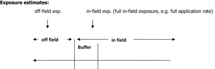
Schematic overview on field scale elements
3.2. Spatial boundaries at the landscape scale
Most reptile species that occur in agricultural landscapes show a high site fidelity. They use off‐field and in‐field areas for feeding, nesting and hibernation. Amphibian species, in contrast, often have migratory behaviour and their feeding and spawning sites are often several kilometres away. Most amphibian species have higher dispersal ability than reptile species that inhabit agricultural landscapes. It is therefore necessary to evaluate the risk to amphibians, not only at the field scale but also at the wider landscape context. Landscape structure is thus particularly important in order to derive a realistic estimate of pesticide exposure to amphibians.
3.2.1. Spatial aspects in relation to the species to be assessed
Amphibian and reptile species differ in the importance of substructuring within larger populations, as well as in their mobility and ability to disperse in the landscape. Many amphibians in particular also exhibit seasonal migrations between breeding and non‐breeding habitats. Seasonal migration is of eminent importance when organisms might be exposed over time to different concentrations, e.g. moving into (and possibly out of) treated fields. Contrary to e.g. non‐target arthropods (NTAs), few, if any, can be defined as having populations entirely within a typical field, and the scales over which a population of amphibians or reptiles might be considered to be contained is larger than a single cropped area (e.g. field). As a result the traditional definitions of ‘in‐field’ and ‘off‐field’ are not easy to apply to these organisms and these should be considered similarly to mobile, NTAs (EFSA PPR Panel, 2015a,b). This means that an individual from a population would not be restricted to single treated or untreated areas and might cover in its range several landscape elements, including in‐field and off‐field areas.
Different habitats may be important at different periods during the life cycle or season, and thus, the coincidence between animals and exposure to PPP needs to be considered in time as well as space. For an individual, this means that it may avoid exposure, or be highly exposed, depending on the availability of the PPP in the environment and the individual's life stage.
Amphibians in particular may have complex, substructured populations (Annex A) and, because they breed in discrete, patchily distributed water bodies, metapopulation ideas have frequently been applied to describe their dynamics (e.g. Gill, 1978; Sjogren, 1991; Hels, 2002; Hels and Nachman, 2002). However, in its strict form, the metapopulation structure is not all‐encompassing and depends on the phenomena of local extinction and of re‐colonisation of all subpopulations. The population structure will very often form a ‘mainland‐island’ complex, in which the ‘island’ populations depend on immigration from the ‘mainland’ for long‐term persistence (e.g. Griffiths et al., 2010). Increased mortality or lowered reproductive success can in all cases reduce re‐colonisation rates and therefore reduce long‐term viability of the overall population. There is a further complexity in the case of mainland‐island situations, in that stressors affecting the mainland will have a much larger impact on the long‐term population state than if they impacted only island populations. Other populations may exist as less structured populations, dispersed over a larger area. In this case, source–sink dynamics (Pulliam, 1988) may be important (Annex A). These are spatial dynamics whereby populations in areas with a negative population growth rate (PGR) are maintained by dispersal from source populations, and are a more general form of the mainland‐island metapopulation structure not needing discrete subpopulations.
3.2.2. Spatial aspects in relation to the landscapes to be assessed
The consequence of large spatial scale of activity and spatially structured populations means that the effects of PPPs on amphibian and reptile populations cannot be considered without considering both landscape structure and the way the animals interact with it. In addition to toxicological variability, the effects of PPPs will therefore depend on the species mobility, seasonal behaviour, population size, meta‐population structure and source–sink dynamics.
Complex spatial dynamics at the landscape scale can be difficult to predict as has been demonstrated for other groups. For example, Dalkvist et al. (2013) found that, contrary to expectations, increasing the area treated with an endocrine disrupter by increasing the area of orchards led to lower relative population impacts and faster recovery. Also surprising was that placing source habitats close to orchards improved recovery and decreased impact due to rescue effects, despite the fact that these narrow habitats were heavily exposed to the pesticide. In carabids, however, these rescue effects can become important depleting dynamics under different circumstances (Topping and Lagisz, 2012; EFSA PPR Panel, 2015a,b). In dispersive spiders, refuges were shown to be able to buffer considerable agricultural mortality impacts (Thorbek and Topping, 2005). As reported by Topping et al. (2014), experimental work with Staphylinidae, Linyphiidae and Carabidae indicates that the appropriate scale for assessing pesticide effects differed between taxa and depended upon the proximity of sources of re‐colonisation as well as dispersal ability. The precise effect of landscape structure interacting with source‐sink dynamics is therefore context dependent and difficult to generalise without more extensive reference work being available.
3.2.3. Spatio‐temporal effects
The exposure to shifting resources and shifting stressors in modern agricultural landscapes may cause declines in species abundance and may also cause non‐equilibrium ecological conditions, where species will suffer conditions of extinction debt (Tilman et al., 1994). Extinction debt means that a species can still be present, but only because it takes an extended time period for the species to become extinct. The ultimate cause of this phenomenon is that the ecological conditions for the species are inappropriate but that, due to spatial and population processes, the extinction time is long, albeit inexorable. This situation is not strictly relevant to the current assessment criteria for PPPs, but is an important part of the spatio‐temporal dynamics of the system. These dynamics are important because an understanding of the state of the system prior to application of the stressor is required as a basis for systems approaches to environmental risk assessment (ERA) (EFSA Scientific Committee, 2016a).
For species with interlinked, spatially structured populations there is an inseparable link between spatial dynamics and temporal dynamics. The metapopulation approach in its simplest form demonstrates that the whole metapopulation should be exposed simultaneously for effective pest control (Levins, 1969); the same will therefore be true of negative impacts on non‐target organisms. It also follows from metapopulation theory that the transient time following perturbation of a population can be long, especially one close to the threshold for persistence, for a species with slow turnover, and in a habitat‐patch network consisting of only a few dynamically important patches (Ovaskainen and Hanski, 2002). Since this considers only a single pulse effect, the implications of multiple applications spanning multiple seasons may be much more serious.
3.2.4. Conclusion
Individual‐level: Exposure to PPP can take place differentially in space and time depending upon the behaviour of the animals coincident with PPP availability in the environment. Therefore realistic risk assessments should take behaviour within a season into account.
Population‐level: Population structure and spatio‐temporal dynamics can have important implications for the evaluation of impacts of PPP on amphibian and reptile populations. A systems approach is therefore recommended by EFSA Scientific Committee (2016a) in order to include both spatial and temporal implications of PPP usage and to take the ecological state of the population into account.
4. Population Dynamics and modelling to support the setting of Specific Protection Goals (SPGs) and ERA
Whatever SPGs are defined for amphibians and reptiles, the main features of interest will be the distribution of animals (where do they occur?), and the abundance of animals (how many are there in the places where they occur?). We may also be interested in their condition. The basics of addressing these issues using population modelling are described in Annex A.
Annex A explains that, for amphibians and reptiles, population modelling taking into account highly detailed environmental and population structure is needed to address adequately the population processes (especially spatial processes) needed for the risk assessment. This section assumes that this context is taken as read.
4.1. Realism and ecotoxicological questions
What we would ideally like to be able to do is to predict the exposure of individuals, their sensitivity, and the effect of exposure, and to predict correctly the impact on the population abundance and dispersion. This is complicated by the fact that complex system properties emerge owing to local space and time feedback mechanisms linking exposure, animal distribution and behaviour, and population responses,. In order to cope with this, a model should include the factors assumed to be important under conditions that might occur in the model's applicable domain. The resulting models should be able to reflect how the internal organisation of populations change and thereby generate representations of the novel behaviour necessary for complex predictions (Topping et al., 2015a).
For spatially structured, long‐lived species with complex life cycles and behaviour such as we see in amphibians and reptiles there is a strong likelihood that simple assumptions about population dynamics and exposure will fail to predict effects accurately due to feedback between factors, e.g. if behaviour causes repeated lifetime exposure due to philopatry of a section of the population. The population will therefore probably need to be modelled as individuals because dispersal behaviour over long lifespans needs to be taken into account. In addition, the dynamic effects of stressors in space and time need to be modelled, applying a regulated stressor assuming year‐on‐year application according to detailed application schedules (including multiple applications).
Simulating the population state realistically prior to addition of the stressor is also a necessity if impacts of the stressor are to be correctly determined (EFSA Scientific Committee, 2016a) and a systems approach is needed for this. Topping et al. (2015b) give an example of the use of a systems model in the context of environmental risk assessment; this spatially explicit, landscape model exemplifies the effects of pesticide application on both abundance and distribution of a non‐target species, not only in fields treated with pesticide but in habitats in unsprayed areas (‘action at a distance’). The model also demonstrated how effects might not be seen for 10 or 20 years, a feature that will not be found in simple demographic models.
This ‘systems’ model trades off generality for realism, and is the basis of the population modelling approach proposed for amphibians and reptiles ERA. Taking this system view also negates the need to consider long‐term recovery separately. PGR will become < 1 if recovery does not occur with year‐on‐year application, and population decline towards extinction will occur. It is also important to note that it is necessary to include species‐specific details in models of this type, e.g. stage‐specific density‐dependence, or behaviour that might change the vulnerability of the population. Hence, significant knowledge is required about the species before these models can be constructed.
The proposed general risk‐assessment framework (Section 7) assumes that models of this type that could be used to assess risks can be built (or exist) for a set of ‘model species’. An example of this approach is provided in Section 7. Selection of species and the criteria used to select exposed vulnerable species are given in Section 2.5.
4.2. Benefits of population modelling exemplified using a model of Triturus cristatus (great crested newt)
This is an illustrative section, demonstrating how detailed population modelling on landscape scales can be used to support the ERA for amphibians. It is based on an individual‐based model of great crested newt (Topping et al., in prep), under the ALMaSS system (Topping et al., 2003). The model builds on previous models and studies of newts. Data inputs rely heavily on Griffiths et al. (2010) and incorporates elements of Griffiths and Williams (2001) and Hels and Buchwald (2001). Development and testing of the model was carried out using pattern‐oriented modelling approaches (Grimm et al., 2005; Grimm and Railsback, 2012), which is becoming the most widely used approach to complex individual‐based simulations in ecology. Similar approaches have been used for the moor frog (Rana arvalis) Dick and Ayllon (2017) and the Houston toad (Bufo houstonensis) (Swanack et al., 2009), the latter also using a pattern‐oriented approach to model development.
There are three main ways in which population modelling can support amphibian and reptile ERA:
Setting specific protection goals
Translation of toxicity data to population‐modelling endpoints
As a higher tier assessment (refinement for population‐level endpoints)
The model has been run using a rather limited and mixed selection of data inputs to illustrate these three points. This is deliberate and the results of the scenarios presented here are not indicative of the results of running a properly defined and agreed great crested newt scenario. For example, all scenarios were run assuming global optimal pond quality, meaning all ponds would be colonised, which is not the case in the real world. The important features of the model are described below, followed by example results and measurement endpoints that could be used to support ERA, including a section describing what needs to be taken into account in order to use a model like this in a realistic scenario.
The great crested newt was chosen since it is one of the six species identified for risk assessment modelling in Section 2.5. This species can be categorised as a species that is highly exposed since it is typically breeding in or around agricultural situations. It is also a low mobility species with seasonal migration to and from breeding sites. It is sensitive to weather conditions and has density‐dependent processes primarily acting at the larval stage. The other five species, which also need to be modelled, have differing profiles and would respond differently to PPP exposure.
4.2.1. Model overview
The model is an agent‐based simulation model working at landscape scale (here taken as 10 × 10 km). It represents individual newts as eggs, larvae, juveniles and adults. Eggs and larvae are aquatic in ponds, juveniles are terrestrial, whist males and females are primarily terrestrial except for breeding periods. The model itself was written in C++ and is part of the ALMaSS simulation system. The code and model are documented using ODdox protocol (Topping et al., 2010a,b), and the documentation is available at https://almassdocs.au.dk/ALMaSSODdox/Newt/index.html.
Life‐stage model overview
Eggs
The female lays eggs in small daily batches. Eggs develop following a day‐degree model until hatching. Each day there is a fixed probability of death per egg (assumed to be predation and other causes not explicitly modelled). In addition, direct mortality can occur as the result of specific events such as acute toxicity of pesticides. In the case of pesticides, these occur as a result of the eggs responding to the concentration of pesticide in the water according to predefined rules (e.g. die when the concentration exceeds a threshold). Maternal transfer could also be implemented since each individual newt has its own time‐varying body burden.
Larvae
When the egg hatches it forms a larva. The larvae are assumed to require aquatic food for growth and if food is available will grow until metamorphosis into a juvenile. The amount of food needed per day is calculated as a function of body size (equating to age). Food is modelled using a simple logistic growth curve (Foodt+1 = Foodt + (Foodt × r × (1 − Foodt/K))) with K and r being specified as input parameters. K is proportional to the area of pond. Food is removed by larval feeding and ‘regrows’ following this curve. There is a probability of daily mortality for unspecified causes similar to the egg, but in addition, there is a probability of dying when Food from the logistic curve is < 50% of K. This probability is inversely proportional to the ratio of Food/K when Food/K < 0.5 (Figure 5). In order to prevent total elimination of larvae in a pond the food level was never allowed to drop below 1% of K. This method means that density‐dependent larval mortality per individual starts when the food levels are < 50% of the maximum food and increases with decreasing food. This is a form of competition intermediate between complete scramble (where all individuals get resources until no resources are left) and contest competition where resources are shared unequally so that some individuals get all the resources they need. The form of competition between individuals can have a large effect on the population dynamic outcome (Smith and Sibly, 1985).
Figure 5.
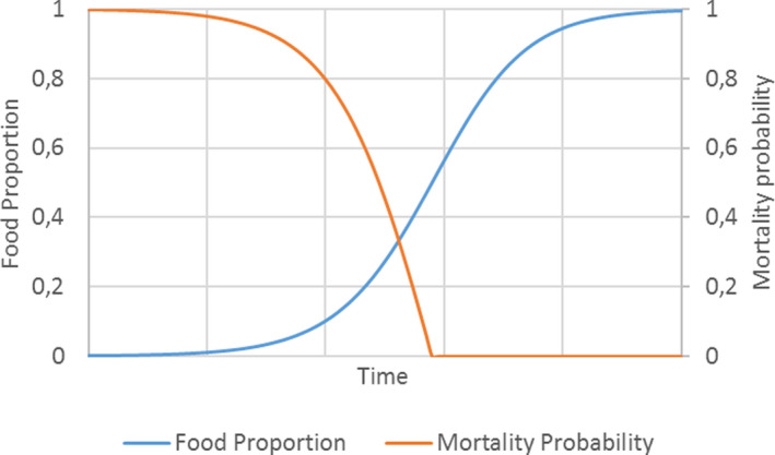
The logistic curve applied to available food for larvae and the related probability of individual larval mortality shown as proportional change in parameter values assuming the food levels grow with time from a very low level at time zero
External events and pesticide concentrations in water can also result in larval death or other responses, as for eggs.
The larval stage is modelled as a fixed period, which triggers metamorphosis into a juvenile when reached.
Juveniles
The juvenile emerges from the pond and disperses into the surrounding area. It moves with a preference for cover habitats and wet areas but will otherwise randomly walk. This has the result that the highest density of newts is near to the pond with decreasing density with distance. The juvenile may encounter other ponds than the home pond as it moves around the landscape and these are remembered.
The juvenile newt can only move around when the humidity is high, which we assume is related to the rainfall and temperature of the preceding days. Roads have associated mortality risks during dispersal; these are flagged and probability tests taken to determine whether or not the juvenile dies.
Apart from dispersal mortality, mortality is based on temperature and precipitation following equations proposed by Griffiths et al. (2010). In addition, the newt responds to pesticides in the environment at its location, e.g. by dying or changing developmental time to adult.
Maturation to adulthood occurs when the newt reaches a specified size. This is partly dependent on the temperature since the newt is assumed not to grow when too cold. On reaching adult size, there is an immediate maturation to either a male or female with equal probability.
Adults
Adults behave in a similar way to juveniles but move relatively less. At the start of the breeding season, the adults will move in a directed manner towards the nearest pond that they have experienced. Once they reach the pond, assuming both sexes are present, the females lay a small number of eggs per day until either the breeding season ends, or the complement of eggs is laid. When the breeding season is over the newts leave the pond and behave the same way as the juveniles, except that movement distance is halved compared to juveniles, the majority of newts staying very close to the pond.
Mortality factors are the same as for the juvenile newt.
Inputs (landscapes, farming and pesticides)
Landscapes used for the model runs were created from combining GIS data with farm subsidy information for Denmark using the methods developed by Topping et al. (2016). These landscapes combine highly detailed landscape structure with accurate representation of farming in terms of crop husbandry and growth. A critical component of the landscape for newts is the pond, which is also available as a GIS layer in Denmark covering water bodies of 5 m2 or more. An example of the distribution of small ponds suitable for T. cristatus is shown in Figure 6. This example shows a high density of ponds, but is not exceptional in a Danish landscape context.
Figure 6.
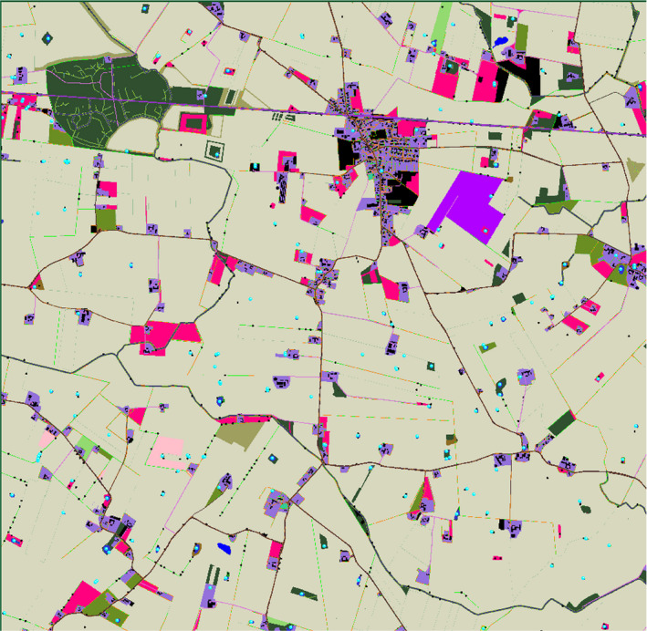
A 5 × 5 km section of the Næstved landscape showing the location of the ponds as light‐blue dots. Rotational fields are shown as light‐brown and it is clear that the vast majority of ponds are in or adjacent to a field where pesticides could be used
Farming was simulated based on the actual farming carried out in the landscape. Polygons representing fields in the landscape map were linked with the farm that manages them and then management typical of that farm type was applied. The management regime was based on data from EU subsidy submission and information on the numbers and types of animals present. The result is a very accurate and realistic representation of crop rotation and crop management into which pesticides could be added.
Pesticides were simulated in two ways. The first way is as a generic pesticide (insecticide, fungicide or herbicide), which had generic properties typical of its type. These pesticides were applied as part of the normal crop management with application frequency and timing based on expert judgement by agricultural consultants. These pesticides have no direct effect on the newt model. The second type of pesticide applied is the focal pesticide for ERA, which is simulated in much more detail. Timing and frequency of application were set explicitly for this pesticide. It was applied at a configurable application rate to a field polygon, with drift into the surrounding area following a user‐defined diffusion curve. After application there was therefore a concentration of pesticide per 1 m2 wherever this was sprayed. This concentration was subsequently degraded by removal of a fixed proportion of the pesticide per day (expressed as a half‐life). Subsequent application to the same area simply adds to the environmental concentration that then decayed.
ALMaSS can represent fate of pesticides in more detail and differentiates fate into vegetation and soil compartments, although only overspray scenarios were used here as detailed fate was not required. The exposure of a newt here was taken to be to 100% of the application rate as overspray (i.e. only those newts in the field or region of drift were affected on the day of spraying). The rate of application was fixed as 1X that required to elicit an LCx response.
All scenarios were run with weather input from central Jutland, Denmark for 1984–2014 unless noted otherwise.
4.3. Linking exposure and effects for long‐term landscape‐scale population RA
Linking exposure and effects in a systems model of the type proposed here is rather different from the traditional approach taken in linking exposure and effects in local short‐term ERA. The systems model enables a dynamic linking of exposure in space and time with the movements of individual animals and behaviours. This means that there is no need to consider a statistical distribution of exposures to select, e.g. the 90th percentile; rather the whole distribution of exposures is simulated and the mean population effect is assessed over whatever spatio‐temporal scales are required for the SPG. This, however, requires that environmental exposure is part of the dynamic simulation. This is easy to do for some exposure routes; in the examples below we have used overspray as being the easiest route to simulate. Other exposure route, however, need to be modelled explicitly within the simulation. This approach was suggested for NTAs for the same considerations of spatio‐temporal effects (EFSA PPR Panel, 2015a,b).
Linking exposure and effects in this way has one critical advantage. It reduces uncertainty resulting from combining two independent distributions (exposure and effects). This may be particularly important if there is an interaction between drivers causing environmental exposure and individual exposure; this could be the case if timing of application coincides with or avoids migratory activity, or if animals are attracted or repelled by a crop that is treated with pesticide (e.g. due to structural cue coinciding with the growth stage for application). Integrated simulation also ensures that only exposure sources that overlap with the distribution of animals in space and time are represented in the measure of impact. Exclusion is automatic since the animals will not be exposed where they do not go (in the model), hence cannot coincide in space or time with PPP in these locations.
The model can use the existing models underlying current environmental exposure estimates. As noted above, the ALMaSS system used for simulating the great crested newt includes drift, environmental decay and the facility to model pesticide movements between vegetation and soil compartments at 1 m resolution for the whole landscape. This is based on simple versions of the exposure models, for example for vegetation the areic mass of substance on the crop canopy, expressed as mass per unit area single sided leaf surface is used. The areic mass can be calculated from the nominal dosage using the fraction intercepted by the crop canopy. Normally, the fraction intercepted depends on the crop development stage and should be obtained from the improved FOCUS interception tables that were published by EFSA in 2014; http://www.efsa.europa.eu/en/efsajournal/doc/3662.pdf). Under dynamic simulation, however, the leaf area index, height and biomass of the crop are simulated daily, and are fed into the exposure calculations dynamically.
4.3.1. Individual toxicity
Effects on the individual are based on the assumption that a given toxicological endpoint is measured over a test with a time component. For example we may have an LC80 measured over 7 days. The response to the pesticide is built into the model by assuming a threshold concentration above which there is a daily probability of mortality. This probability (p) is calculated from (1 − m) = (1 − p)d, where m is the proportion assumed to die (e.g. 0.8 for 80% mortality over the test period of 7 days) and d is the number of days over which the test was carried out. If the newt finds itself in a 1 m2 grid cell with an environmental concentration above the trigger, then it is assumed to die with probability p.
This approach is called the stochastic death model in GUTS toxicodynamics/toxicokinetic (TK/TD) modelling (see Ashauer et al., 2015) and can be contrasted with the individual threshold approach, which sets an individual threshold above which death is certain. The implication of this choice is difficult to determine at the system level, but stochastic death has a larger probability of killing all exposed animals if multiple exposure occurs whereas at low exposure levels the individual threshold approach leads to higher effects. Both approaches also make the assumption that an individual that survives exposure does not have any subsequent change in sensitivity (e.g. if it was weakened by the first exposure it might be more sensitive to future exposure). There is no obvious reason to choose one or other approach; however, it is important to make an informed, transparent choice in each case.
4.3.2. TK/TD modelling
For a better linking between a dynamic exposure profile and the effects induced on individuals, simulations with TK/TD models could be developed. This would dynamically link exposure, the movement of animals and their exposure producing input to the TK/TD models. Toxicokinetics refer to the processes that influence internal exposure of individual organisms (e.g. diffusion over the organism surface, or active uptake e.g. via membrane transporters or via food). Toxicodynamics refer to the processes that lead to their damage and/or mortality. The current newt model has a simple one compartment (whole organism) TK model that keeps track of internal body‐burden and elimination rates can be specified, exposure patterns in space and time being dynamically simulated as described above with a daily resolution. This is currently very simple and assumes a constant elimination proportion (the simplest TK model). A very useful advance would be to link the individual, temporal exposure profiles with the metabolism of the animals. This would incorporate an element of risk assessment considered to be specific and important for amphibians and reptiles, i.e. poikilothermy and its influence on pesticide effects. Inclusion of this linkage would change the rate at which pesticides were eliminated, dependent upon temperature‐driven metabolism, improving the toxicokinetics. Naturally, more detailed toxicodynamics would increase the potential realistically to combine different routes of exposure and even different toxic effects (e.g. direct effects on skin and subsequent effects on other organs in the body).
Direct integration in the simulation would further reduce uncertainty by integrating exposure with ecology and behaviour with TK/TD to create population‐level effects. Like integration of exposure and effects, the detailed patterns of individual exposure created by animals moving around in the simulated environment and being exposed would drive the TK/TD models directly, thus removing the need to provide statistically generated exposure profiles.
There are no significant technical issues in developing TK/TD models and directly integrating them in simulations like the great crested newt model. There are currently, however, few data on toxicity for these groups (see Section 10), and even less data to enable parameterisation of TK/TD models. TK/TD models are therefore not feasible currently without further data.
4.4. Endpoints
4.4.1. Impacts
Measuring population impact requires a no‐pesticide situation against which to compare pesticidal effects. This is termed the baseline and represents a model identical in all respects to the scenario used to test a pesticide except that the particular pesticide under evaluation is not applied. A baseline is required for each scenario, and typically a range of baseline scenarios are used to represent the range of situations a population may be in (for example, low resilience population in an intensive agricultural landscape, and a widespread resilient population in an extensive landscape). This range of scenarios is needed because it is difficult to identify in advance which baseline will react most strongly to the combination of pesticide and SPGs. The baseline population size will fluctuate in time, and this defines the normal operating range of the population for that scenario. To create the baseline the model needs to be carefully tested to determine whether it performs closely to the real world. Examples of this can be seen for partridges, hares, voles and skylarks (Topping et al., 2010a,b, 2012, 2013). The newt model used here has not as yet undergone this degree of testing. Although the same strategy of using pattern‐oriented modelled to develop the model was used, the data available for the newt was not of the same quality or quantity as for the previous species; hence, the model developed is simpler and uncertainty is relatively high.
If the newt model represents the real world well, then we can assume that the population trajectory described by running the model with a current agricultural scenario represents the current state of the population. An example of single runs for the Næstved and Mors landscape is shown in Figure 7.
Figure 7.
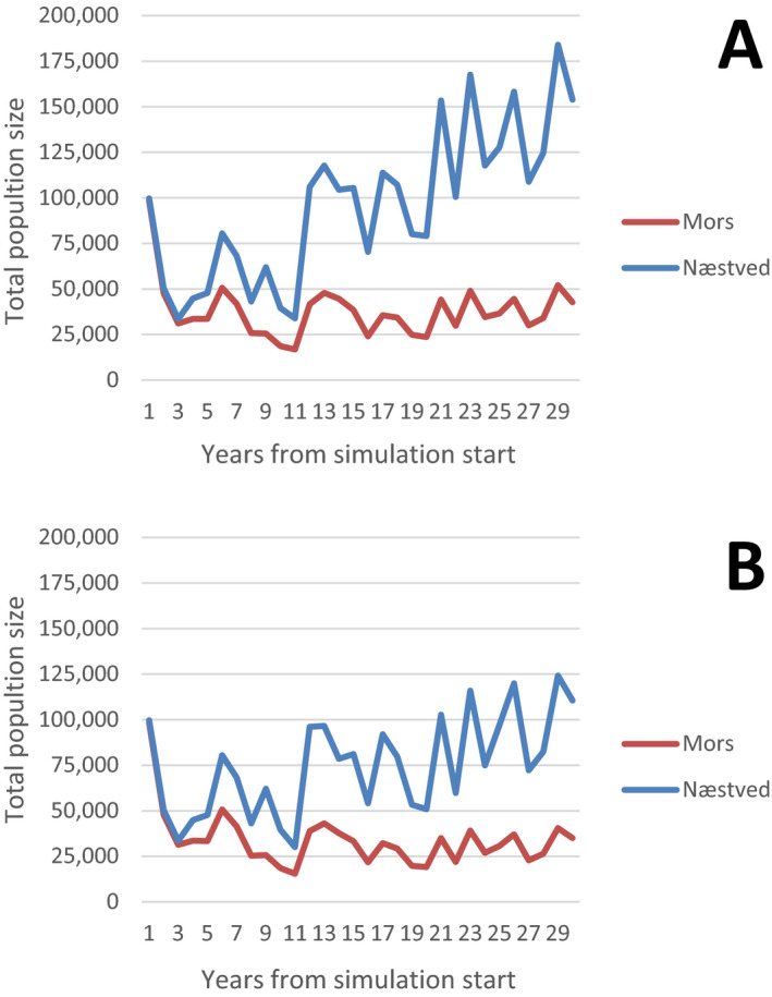
Total adult female population size for two simulation runs on two different landscapes (Mors & Næstved). Both simulations were started with 100,000 individuals but clearly have very different carrying capacities. (A) Without pesticide (baseline); (B) The same simulation but with addition of a pesticide LC 100 from year 11 onwards
Adding the pesticide to the (otherwise unchanged) scenario alters the population curves (Figure 7B). The heights of the curves are different though the basic shapes are the same as the baseline; this is because the other main drivers of population size (farming, landscape and weather) are identical between scenarios. Comparison of the raw numbers between runs is, however, difficult and the population size relative to the baseline is used to facilitate easy comparison (Dalkvist et al., 2009). This allows comparison of the baseline and pesticide scenario directly (Figure 8).
Figure 8.
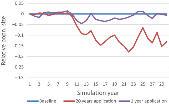
LC 100 overspray scenario on the Mors landscape assuming application to winter wheat, spring barley and oilseed rape following the spraying schedule described in Table 9
The overall population impact is one endpoint useful to compare changes in population size. Another endpoint can, however, be considered as introduced by EFSA PPR Panel, 2015a,b, for NTAs: this is the abundance occupancy ratio (AOR) index (Hoye et al., 2012). The AOR index describes the change in abundance (population density where the population occurs) and occupancy (the relative proportion of the landscape occupied by the population). As with overall population impact, these measures are relative to a baseline. The AOR index can be plotted easily and provides information on both abundance and dispersion. Figure 9 shows an example of changes in occupancy and abundance for increasing LCx overspray scenarios in the Næstved landscape. These scenarios assume application of the pesticide to be evaluated to winter wheat, spring barley and oilseed rate grown to maturity at standard rates following the application schedule in Table 9. The effect of increasing toxicity is clearly seen both in terms of changing newt population, abundance and newt distribution, which in this case shows a close to linear response.
Figure 9.
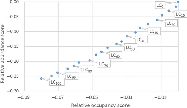
Occupancy and abundance scores for LC x overspray scenarios for the last decade of a 20‐year application on the Næstved landscape, assuming application to winter wheat, spring barley and oilseed rape following the spraying schedule described in Table 9
Table 9.
The timing of the day of application for each of three pesticide applications for the three crops used in ERA scenarios. For winter wheat and spring barley, the probability of pesticide application was independent (e.g. 3 × 50%). For oilseed rape, applications were dependent upon previous applications, i.e. 30% of the 21% that applied the first application will apply the second
| Crop | Application 1 | Application 2 | Application 3 |
|---|---|---|---|
| Winter Wheat | 50% on 15 May | 50% on 1 June | 50% on 14 June |
| Spring Barley | 35% on 15 May | 35% on 1 June | 35% on 14 June |
| Oil Seed Rape | 21% on 15 April | 30% on 1 May | 70% on 15 May |
4.4.2. Year‐on‐year effects
Note that, depending upon the size of acceptable impact, it may be difficult to identify a population response from a single year application. Figure 10 shows that for LC5 it took three years before the population impact was observable in the model, but after that period the effect was clear, averaging 2.5% and never returning to the baseline.
Figure 10.
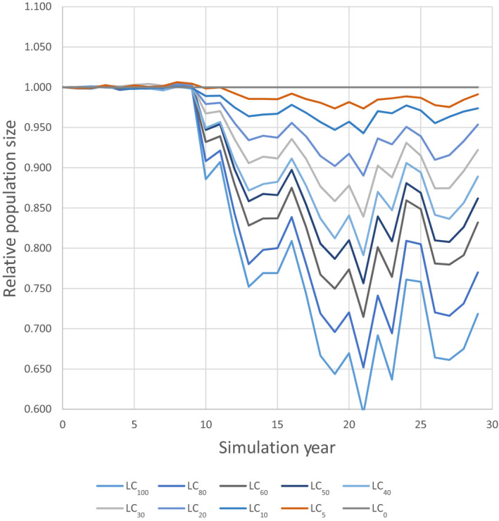
Change in population size for LC x overspray scenarios of a 20‐year application on the Næstved landscape, assuming application to winter wheat, spring barley and oilseed rape following the spraying schedule described in Table 9
Impact can be measured following a single pulse or as the result of year on year application. These two situations are compared for Næstved (Figure 11). In this case, a single year impact of the LC100 overspray scenario was a 9% reduction in population size but continuous use led to a 20% population decline, after 10 years.
Figure 11.
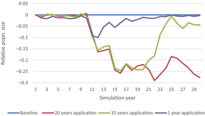
LC 100 overspray scenario 1‐year, 10‐year and 20‐years application on the Næstved landscape assuming application to winter wheat, spring barley and oilseed rape following the spraying schedule described in Table 9
4.4.3. Recovery
Recovery might not need to be considered if only negligible effects are permitted, depending on the SPG considered. If we are then comparing annual population status as described above, then there is no need to consider within season recovery since, if recovery does not occur, there will be population impacts. If population impacts are allowed, however, recovery should be possible (unless PGR < 1).
Like impact, assessing recovery can be done by comparing changes relative to a baseline condition (see Figure 11). This example is based on a 100% mortality overspray scenario for the Næstved landscape following application to all winter wheat, spring barley and winter oilseed rape fields according to Table 9. Each scenario has a 10‐year non‐application phase followed by a 1, 10 or 20‐year application of the pesticide during a total of 30 years of simulation. Note that recovery seems to occur in the 10‐year application scenario by year 25, but full recovery does not actually take place in the 10 years following cessation of pesticide application. Even after one year's application, recovery takes 15 years in this system. After 10 years of application and after 10 years recovery the population is still at 95% of its original size.
4.4.4. Population growth rate (PGR) and relative PGR
As discussed earlier in this section and in Annex A, PGR is the single, most critical metric for population status. If PGR < 1, the population will decline. A long‐term decline that is a result of the regulated stressor is not acceptable for a non‐target reptile or amphibian population because the SPG cannot be sustained over time.
It may be, however, that PGR < 1 before the pesticide is applied. Risk managers need to consider how to deal with this scenario, which may be a consequence of modern agricultural practice altering landscapes or an indirect effect on, e.g. prey. Another scenario is where PGR < 1 over a short‐time scale but PGR ≥ 1 over a longer time period. In order to help risk managers to deal with both these scenarios, we suggest the use of a relative PGR in a similar way to measuring the relative impact against the relevant baseline. Assuming we have an ‘acceptable’ population decline after a period of pesticide application, what we are interested in knowing is whether the population has stopped declining relative to the baseline under continued pesticide use. This is difficult to assess by eye from a population‐impact graph such as Figure 11. However, regressing the change in population size per year for fixed periods allows a statistical comparison. Figure 12 shows the three 10‐year periods change in relative population size plotted against year from start of each 10‐year period. It is clear that the first 10 years of pesticide application (Decade 2) cause the decline, after which the population seems to stabilise at a level about 75% less than its original size (Decade 1).
Figure 12.
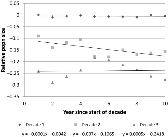
Three 10‐year time series created by splitting the result of the 30‐year run with 20 years application from Figure 11 into three decades then fitting a linear regression of relative population size against year within each decade. The equations shown for each decade indicate the slope of the relative PGR for that decade
4.5. Translation of toxicity data to population endpoints
The key advantage of population modelling is that it takes existing data as input (which can include endpoints of lower tier testing), and translates this into the key, population‐level endpoints of distribution of animals in space and time and population persistence (i.e. abundance, occupancy and PGR). Additional laboratory tests, specifically aimed at the modelling, are not required.
To exemplify the way in which a lower‐level screening test might be done we have used the newt model on the 10 landscapes developed by Topping et al. (2016), assuming the LC100 overspray scenario on winter wheat, spring barley and oil seed rape. Figure 13 shows the population size, abundance and occupancy changes for all 10 landscapes. It is clear that the magnitude and pattern of responses varies with the landscape context. In some landscapes, abundance is very sensitive in others occupancy responds most strongly (N.B. with –1 occupancy score, there must also be a –1 abundance score and vice versa).
Figure 13.
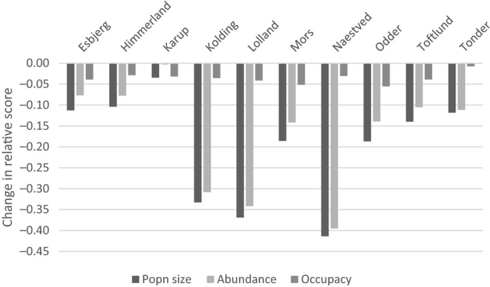
Change in relative population size, abundance and occupancy when running the LC 100 overspray scenario on 10 different Danish landscapes
Ideally, many more landscapes should be generated representing the range of landscape/farming possibilities from the region being considered, which is now technically easy to achieve with data available in Denmark (Topping et al., 2016), and also for the rest of the EU if data‐accessibility issues can be resolved. When more landscapes are available, cases applying a percentile approach to the population‐level endpoints would allow selection of one or more representative landscapes as realistic worst‐case scenarios. If we assume that for our case this landscape is the Næstved landscape, then we can read off the impact of the pesticide based on its LCx from Figure 9, and compare this to the SPG level of concern.
This approach means that a year‐on‐year effect of pesticide use can be calculated using toxicity endpoints, fate, and application schedules from existing testing,. In this case we used LCx, but precisely the same approach can be used for chronic endpoints if chronic toxicity endpoints are incorporated into the models. Naturally, the results of different modes of action will differ; therefore, the models need to be run for each relevant regulatory scenario.
4.6. Supporting SPG definition using modelling results
One of the problems of landscape population‐level ERA is that the SPGs require re‐formulating. Simulation of populations in space and time allows for an exploration of the population‐level impacts of stressors and therefore the range of responses to pesticide scenarios. Given this range of response, the setting of protection goals can be achieved by considering the acceptability of impacts.
Although the setting of population‐level effects is a risk manager decision, it is useful if a science‐based approach can provide as much information as possible to aid the decision.
Before considering SPGs the relevance of the impacts measured should be determined. In the Næstved landscape simulations, we saw occupancy changes of up to less than 10% but this should be considered against the background of what might be a maximum realistic reduction in this landscape. To demonstrate an extreme overspray situation, the Næstved landscape was also run with all crops receiving three applications (including farmed grasslands) and LC100. This gave an occupancy reduction of 28% and at the same time a 77% abundance with an overall population size reduction of 83% (not shown). At this point, the population was stable, but restricted to breeding in non‐agricultural habitats, having been eradicated as a breeding population in agricultural areas. Some individuals were present in the agricultural areas each year, but these came from non‐agricultural parts of the landscape as emigrants (action at a distance). This scenario therefore represents the maximum level of impact that application of overspray to agricultural areas could achieve.
Having scaled the impact, combination of the following endpoints can be used to the thresholds for the SPG for landscape‐scale populations:
Impact on density and distribution. In our standard scenario assuming LC80, there was a reduction in occupancy of 6%, which is 6/28 or 21% of the maximal impact. In the rest of the landscape, the population was still extant, but at mean densities that were 20% lower.
The long‐term population impact. In this case, relative PGR was stable after 10‐years of application, which would not be considered to present a risk of long‐term total landscape extinction (although this might not be the case for other landscapes or model settings).
The potential for recovery at the population level. Using these results as an example, we might consider that population impacts could be tolerated if recovery at the population level is fast. If, however, indications are that recovery after impact is very slow, only negligible impacts would be likely to be acceptable (as in this example, Figure 11).
In order to define the SPG, these three endpoints need to be combined and translated to impacts on ecosystem services for the range of toxicities and modes of actions possible, and then tabulated. These impacts, e.g. a 20% reduction in occupancy and 21% abundance that is long‐term stable but lasts 15 years after cessation of application, need to be translated to the effects the impacts will have on the services supported by the SPGs (although this is challenging). If an unacceptable level of impact on service can be identified, the corresponding level of toxicity can be determined from such a table of combined effects (see Section 7.10).
4.7. Refinement of model inputs
The assumptions in the scenarios above include the typically used proportion of time spent in crop (PT), i.e. the model calculates the likelihood of a newt being in the crop during application as part of the normal calculation integrating behaviour and development of the newts. Consequently, refinement of the species model itself is not desirable, but refinement of exposure can form a part of a higher tier assessment for the modelling endpoints. Note, however, that in the scenarios used here, exposure was based on the newt being exposed to the full field rate as overspray, but in these scenarios there was no toxicity to any other stage, and exposure to environmental residues after spraying and in ponds was considered to be zero (see below for more realistic assumptions). While refinement of individual exposures is possible, for population‐level effects it is critical that all stages and exposure routes are taken into account concurrently if realistic effects are to be predicted.
One key aspect of the scenarios that needs to be considered for long‐term population models is the weather input. The newt model is highly sensitive to weather data. Figure 14 shows the data from the LCx experiment but with additional points created by running LCx scenarios under weather from 1950 to 1980 instead of the last 30 years’ weather. The weather clearly has a large impact on the vulnerability of the population to pesticide effects; therefore, a careful consideration of weather is needed in any regulatory scenario.
Figure 14.
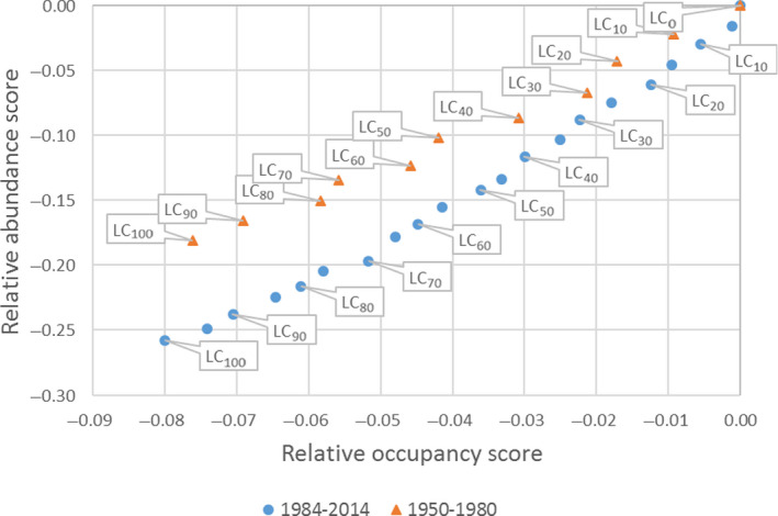
AOR scores for the newt overspray scenario using application to wheat, barley and oilseed rape (combined crop pattern) but different assumptions of overspray LC x under two weather regimes
These newt model scenarios did not utilise all possible features of the ALMaSS simulation system. In particular, assumptions about timing and frequency of application, subsequent exposure and environmental fate of pesticide use worst‐case settings. These assumptions could be refined in higher tier assessments and this could be achieved in the current model for the terrestrial stages; however, realistic estimates of pesticide concentration in pond water are not part of the ALMaSS framework and would need to be developed for pond‐living species before this type of model could be used.
It is important to note that population‐modelling endpoints should be kept separate from other endpoints because confounding of the population‐modelling results can occur. For example, the LC5 year‐on‐year results showed that it is possible to obtain no observable effect (e.g. in a 1‐year field test) but still have a population‐level effect after year‐on‐year use. Figure 15 shows an example where LC5 produces no observable population impact for 3 years after application but subsequently there is a clear impact. These effects would be extremely challenging to observe in the field due to limits of detection. Refinement of the population model with field testing is therefore not possible. Similarly, since the model explicitly incorporates the behaviour that changes the time spent by the newts in crop (often referred to as PT), refinement of toxicity data using PT is also not possible because it would result in double refinement. Hence, the criss‐cross model (Section 7.3) cannot be applied to population‐modelling endpoints. However, note that this does not mean no refinement of parameters related to exposure in the model, only that double refinement must be avoided.
Figure 15.
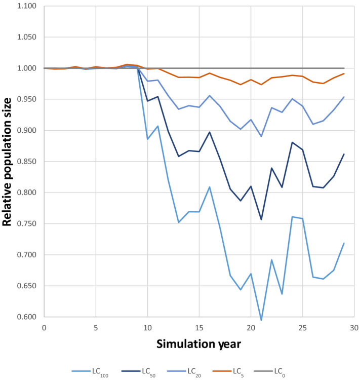
Time series for four relative population sizes resulting from LC x/LC0 with pesticide application starting in year 10
4.8. Developing realistic scenarios
The scenarios and model used here are for illustrative purposes only; no numbers or results should be taken as indicative of future trigger values or modelling approaches, or indeed parameter values since many were chosen arbitrarily for this exercise. A number of steps and improvements to the model and scenario are needed before the model could be used in practice. These are primarily the following:
More detailed testing and evaluation of the newt model is needed.
The pond resources are assumed to increase with pond area (up to a maximum). In reality, the quality of resources could vary with factors such as soil type, and this would affect patterns of spatial density dependence.
Pesticide‐exposure module needs to be extended to include realistic or agreed methods to implement pesticide concentrations in ponds, including the use of monoculture scenarios as extreme limit scenarios.
Exposure routes linking environmental concentration to the body‐burden of pesticide in the newt need to be defined and included.
The result of exposure needs to be carefully considered since exposure may be a daily or regular occurrence in the lifetime of a newt and the combining of probabilities mathematically may over‐ or under‐estimate effects.
Landscape, weather and farming scenarios need to be considered carefully to be representative of the region under consideration.
Ideally, scenario and model development should be part of an interactive model cycle, fed by data from the real world, e.g. via monitoring.
Development of landscape and farming simulations for the regulatory zones in EU is needed to support the model in these zones, and similarly for any individual country that may wish to use the model.
4.9. Conclusions and recommendations
4.9.1. Conclusions
Population structure and spatio‐temporal dynamics can have important implications for the evaluation of impacts of pesticide on amphibian and reptile populations. A systems approach is therefore recommended, for inclusion of both spatial and temporal implications of pesticide usage and to take the ecological state of the population before application of pesticides into account (EFSA Scientific Committee, 2016a).
Spatially explicit, individual‐based modelling at landscape scales is an important part of the ERA toolbox for amphibians and reptiles. It should be used to help set the tolerable magnitude of effects for SPG, to translate toxicity data into population‐modelling endpoints, and as a higher tier assessment tool.
Precise context for application of the models requires careful consideration. The regulatory scenarios need to consider all factors; in particular, landscape structure and weather have a large impact on the outcome of the long‐term risk assessment.
The threshold limits of changes to population‐level endpoints that correspond to unacceptable impacts on the SPG need to be identified. This should not be done on an individual endpoint basis but combining abundance, occupancy and changes in growth rate.
First indications from model development are that recovery in terms of landscape occupancy may be very slow for the great crested newt, and this is probably true for other species with similar limited dispersal ability.
4.9.2. Recommendations
The suggested risk assessment scheme (Section 7) requires the risks of intended uses of pesticides to be assessed at landscape scale. In order to obviate the need for direct running of complex models at lower tiers, it is recommended that these scenarios are developed as a set of prerun simulations and made available with an interface for input of standard toxicity and usage data to provide a quick look‐up function for lower tiers.
Landscape‐scale, spatially explicit mechanistic models need to be developed and tested for the six focal species suggested for the assessment of amphibians and reptiles. These should include:
Mechanistic modelling of dispersal, reproduction and mortality factors for all life stages;
The potential to introduce a wide range of impacts of PPP in terms of modes of action, exposure and regulatory scenarios;
Spatial and temporal representation of resource distributions;
Realistic pesticide‐exposure modules including realistic or agreed methods to implement pesticide concentrations in ponds;
Exposure routes linking environmental concentration to the body burden of pesticides need to be defined and included, as well as inclusion of a suitable representation of multiple exposure events for an individual;
Population‐modelling endpoints should include the abundance of the animals, their distribution and relative change in PGR as a result of application of the PPP. The latter takes into account long‐term impacts, which can be difficult or impossible to see using other approaches.
It is recommended that the use of TK/TD models be considered to represent better the exposure of amphibians and reptiles when the terrestrial stages move in and out of contaminated areas, as well as being exposed to multiple applications. Detailed, temporal exposure profiles suitable for TK/TD modelling can be generated from the individual‐based population modelling and incorporated directly into the landscape‐scale models. Collection of data to drive TK/TD modelling must be prioritised as part of future research.
5. Defining specific protection goals for amphibians and reptiles
5.1. General considerations
Regulation (EC) No 1107/2009 (European Commission, 2009) defines general protection goals that aim at protecting inter alia non‐target organisms, biodiversity and ecosystems. It is thus necessary to define specific protection goals (SPGs) aiming at implementing this general protection into explicit and viable mandates for risk assessors, who need to know what to protect, where to protect it and over what time period. Final decisions on the choice of specific protection goals need to be made in consultation with risk managers.
The role of EFSA's risk assessment is to propose possible SPG options based on environmental and ecological criteria (and related exposure assessment goals), acknowledging existing general protection goals described in the relevant EU Regulation or Directive and regulatory data requirements. These SPG options, as well as a description of the possible environmental consequences of each option, should be proposed and discussed with risk managers. Risk managers should select SPG options, or to amend SPGs proposed by risk assessors. Agreed SPG Options should form the basis of ERA decision schemes, which will be included in subsequent guidance documents. The choice by risk managers belonging to the European Commission (DG SANTE) and EU Member States is based on a cost‐benefit evaluation ‐ also considering economical and political criteria and acknowledging consequences for human wellbeing (health and economic benefits) and environmental costs.
For the purpose of this opinion on amphibians and reptiles, the Panel considers it appropriate to examine which protection goals are already in place regarding the risk of aquatic and terrestrial vertebrates exposed to intended uses of PPP. Additionally, the procedure to define specific protection goals as developed by EFSA in consultation with stakeholders (EFSA PPR Panel, 2010) and in the Guidance of the EFSA Scientific Committee (EFSA Scientific Committee, 2016b) is followed. Understanding the contribution of amphibians and reptiles to ecosystems can help risk managers in the decision on which SPG option to choose and how to prioritise protection measures. Moreover, it enables the understanding of interactions and ultimately the prediction of biotic and abiotic changes associated with the potential loss of species (Şekercioğlu et al., 2004; Hocking and Babbit, 2014a,b).
The aim is to propose SPG Options that
take current protection goals for non‐target vertebrates into account,
refer to the ecosystem services that amphibians and reptiles provide for mankind, and
consider especially the endangered status of several amphibians and reptiles species in European agricultural landscapes
5.2. Legislative framework in place
The legislative framework currently in place addressing the risk for amphibians and reptiles exposed to PPPs is reviewed and given below.
The general protection goals for non‐target organisms exposed to intended uses of PPP are outlined in the EU Regulation No 1107/2009. The regulation states in Article 4 on the approval criteria for active substances the following:
(e) it shall have no unacceptable effects on the environment, having particular regard to the following considerations where the scientific methods accepted by the Authority to assess such effects are available:
-
(i)
its fate and distribution in the environment, particularly contamination of surface waters, including estuarine and coastal waters, groundwater, air and soil taking into account locations distant from its use following long‐range environmental transportation;
-
(ii)
its impact on non‐target species, including on the ongoing behaviour of those species;
-
(iii)
its impact on biodiversity and the ecosystem .
Regarding the requirements for data that are to be provided for the assessment of the effect of active substances and PPP on non‐target organisms, Directive No 283/2013 (European Commission, 2013) demands i.a., that ‘the information on the active substance, taken together with the information concerning one or more plant protection products containing the active substance […] shall be sufficient to: […]
-
(d)
permit an assessment of the impact on non‐target species (flora and fauna), including the impact on their behaviour, which are likely to be exposed to the active substance , its metabolites, breakdown and reaction products, where they are of toxicological or environmental significance. Impact can result from single, prolonged or repeated exposure and can be direct or indirect, reversible or irreversible;
-
(e)
evaluate the impact on biodiversity and the ecosystem;
-
(f)
identify non‐target species and populations for which hazards arise because of potential exposure;
-
(g)
permit an evaluation of short and long‐term risks for non‐target species, populations, communities and processes ;
In submitted ecotoxicological studies (Section 8) “The potential impact of the active substance on biodiversity and the ecosystem, including potential indirect effects via alteration of the food web, shall be considered”.
While it is stated that effects on terrestrial vertebrates other than birds “[…] shall be derived from the mammalian toxicological assessment based on the studies referred to in Section 5 (Toxicology)”, a separate Section (8.1.4) addresses “Terrestrial vertebrate wildlife (birds, mammals, reptiles and amphibians”. Here:
Available and relevant data, including data from the open literature for the active substance of concern, regarding the potential effects to birds, mammals, reptiles and amphibians (see point 8.2.3) shall be presented and taken into account in the risk assessment.
The mentioned Section 8.2.3 addresses the question whether “[…] the active substance is a potential endocrine disruptor in aquatic non‐target organisms according to Union or internationally agreed guidelines. […]”
In addition to the above, Regulation 284/2013 specifies the data requirement for plant protection products. For effects of PPP on “ Other terrestrial vertebrate wildlife (reptiles and amphibians) ”, it is stated that “where it cannot be predicted from the active substance data and, if relevant, the risk to amphibians and reptiles from plant protection products shall be addressed”.
The EU Regulation No 546/2011 implements EU Regulation No 1107/2009 as regards to the uniform principles for evaluation and authorisation of plant protection products. The evaluation of PPP impact on non‐target species is presented in Section B.2.5.2. It should be noted that amphibians and reptiles can be subsumed in ‘other terrestrial vertebrates’.
When calculating toxicity/exposure ratios Member States shall take into consideration toxicity to the most sensitive relevant organism used in the tests.
2.5.2.1. Member States shall evaluate the possibility of exposure of birds and other terrestrial vertebrates to the plant protection product under the proposed conditions of use; if this possibility exists they shall evaluate the extent of the short‐term and long‐term risk to be expected for these organisms, including their reproduction, after use of the plant protection product in accordance with the proposed conditions of use.
-
This evaluation shall take into consideration the following information:
the specific information relating to toxicological studies on mammals and to the effects on birds and other non‐target terrestrial vertebrates, including effects on reproduction , and other relevant information concerning the active substance as provided for in the Annex to Regulation (EU) No 544/2011 and the results of the evaluation thereof;
all relevant information on the plant protection product as provided for in the Annex to Regulation (EU) No 545/2011, i ncluding the information on effects on birds and other non‐target terrestrial vertebrates ;
where relevant, other authorised uses of plant protection products in the area of envisaged use containing the same active substance or which give rise to the same residues.
-
This evaluation shall include:
the fate and distribution, including persistence and bioconcentration, of the active substance and of relevant metabolites, breakdown and reaction products in the various parts of the environment after application of the plant protection product;
the estimated exposure of the species likely to be exposed at the time of application or during the period that residues are present, taking into account all relevant routes of exposure such as ingestion of the formulated product or treated food, predation on invertebrates, feeding on vertebrate prey, contact by overspraying or with treated vegetation;
a calculation of the acute, short‐term and, where necessary, long‐term toxicity/exposure ratio. The toxicity/exposure ratios are defined as respectively the quotient of LD50, LC50 or non‐observable effects of concentration (NOEC) expressed on an active substance basis and the estimated exposure expressed in mg/kg body weight.
Regarding the decision making (Section C), the Regulation states that, for non‐target species:
2.5.2.1. Where there is a possibility of birds and other non‐target terrestrial vertebrates being exposed, no authorisation shall be granted if :
– the acute and short‐term toxicity/exposure ratio for birds and other non‐target terrestrial vertebrates is less than 10 on the basis of LD 50 or the long‐term toxicity/exposure ratio is less than 5 […]
unless it is clearly established through an appropriate risk assessment that under field conditions no unacceptable impact occurs after use of the plant protection product in accordance with the proposed conditions of use.
Also relevant for amphibians is the indication for decision making regarding aquatic life stages:
2.5.2.2. Where there is a possibility of aquatic organisms being exposed , no authorisation shall be granted if:
– the toxicity/exposure ratio for fish and Daphnia is less than 100 for acute exposure and less than 10 for long‐term exposure, or
– the algal growth inhibition/exposure ratio is less than 10, […]
unless it is clearly established through an appropriate risk assessment that under field conditions no unacceptable impact on the viability of exposed species (predators) occurs — directly or indirectly — after use of the plant protection product in accordance with the proposed conditions of use.’
The so‐called ‘unless clause’ gives the opportunity for a refinement of a risk that has been indentified at lower tier assessment steps. Interestingly, for the non‐target terrestrial vertebrates, no restriction is made on the species at risks that need to be addressed. The consideration of the risk for aquatic organisms points especially to ‘predators’.
5.3. Defining SPGs according to the ecosystem service concept
In the relevant PPR Panel Opinion (EFSA PPR Panel, 2010) and the Guidance of the Scientific Committee (EFSA Scientific Committee, 2016b, several steps are proposed in order to identify and to justify specific protection goals for aquatic and terrestrial organisms that may be affected as non‐target organisms by use of PPPs. These steps are needed in order to ‘delineate the environmental components to protect, the maximum impacts that can be predicted and, in the case of regulated products, tolerated, over what time period and where.’ (EFSA Scientific Committee, 2016b. The Guidance Document on protection goals (EFSA Scientific Committee, 2016b aims at harmonising the approach to define SPGs across the different areas of EFSA's responsibility.
The approach follows three sequential steps: (1) the identification of relevant ecosystem services; (2) the identification of service providing units (SPUs) that support relevant ecosystem services and (3) the specification of the level/parameters of protection of the SPUs, using interrelated dimensions.
This last step involves the specification of the ecological entity and attribute to protect and the magnitude, temporal scale and spatial scale of the biologically relevant effects for all potential stressors followed by the definition of what is tolerable after intended uses of PPP.
SPG options have to be proposed for each combination of SPU and ecosystem service.
5.3.1. Ecosystem services driven by amphibians and reptiles in agricultural landscapes
The first step in the definition of SPGs is the identification of ecosystem services that are considered important and are provided by agricultural ecosystems. By means of describing services that mankind receives from ecosystem performance, the value of abstract ecological entities and processes become more explicit. Several classification schemes for ecosystem services have been proposed, e.g. MEA, 2005; CICES (http://cices.eu/) and TEEB (http://www.teebweb.org/). In this Opinion, in accordance with other Opinions and Guidance of EFSA on the topic (EFSA PPR Panel, 2010; EFSA Scientific Committee, 2016a), a list of ecosystem services based on the Millennium Ecosystem Assessment (MEA) source has been used since it is widely recognised and adopted. The MEA (2005) noted, however, that ‘modifications of ecosystems to enhance one service generally have come at a cost to other services due to trade‐offs.’ The impacts of these trade‐offs should be clearly described also for ecosystem services in agricultural landscapes, so that risk managers can decide whether and to what extent costs of trade‐offs should be tolerated. In this respect, MEA (2005) claims that ‘many of the costs of changes in biodiversity have historically not been factored into decision‐making’.
Based on the assessment of existing knowledge and published reviews (e.g. Hocking and Babbit, 2014a,b; Valencia‐Aguilar et al., 2013), nine ecosystem services were identified as being driven by amphibians and reptiles in the agricultural landscape. These services (and their classification in brackets) are:
Genetic resources, biodiversity (provisioning and supporting). Amphibians and reptiles contribute highly to the biodiversity of agricultural landscapes. Several species with (part of) their habitat in agricultural landscapes have been classified as being endangered in Europe and/or are protected by law.
Education and inspiration, aesthetic values and cultural diversity (provisioning). Amphibians and reptiles species are highly valued in human culture. Their aesthetic value is widely acknowledged and they are used as strong symbols in visual arts and literature.
Pharmaceutical resources (provisioning). Amphibians and reptiles species provide compounds with specific applications in medicine.
Food (provisioning). Amphibians and reptiles provide food resources to mankind. Frog legs especially are consumed not only worldwide, but also in parts of Europe.
Nutrient cycling (supporting). The cycling of nutrients in water bodies and soils is the basis for life. Amphibians and reptiles contribute especially with digging to the mixing of soil and sediments, and shift dead organic matter from above‐ to below‐ground and from terrestrial to aquatic habitats, finally enhancing nutrient mineralisation.
Soil structure formation (supporting). Digging activities of amphibians and reptiles in terrestrial habitats contribute to the formation of soil structure. Tadpoles in ponds affect sedimentation processes.
Pest and disease outbreak control (regulating). Amphibians and reptiles can contribute to the reduction of pests in agricultural systems. Preying on, e.g. mosquito larvae alters diseases transmission, especially by amphibians in ephemeral wetlands.
Invasion resistance (regulating). Autochthonous amphibian and reptile species might provide invasion resistance to alien species.
Food provision, food‐web support (supporting). Amphibians and reptiles are important parts of aquatic and terrestrial food webs. Being themselves predators or herbivores, they provide secondary production and support biodiversity at higher trophic levels.
5.4. Special consideration of endangered species
As noted in Section 2, a high percentage of amphibian and reptile species is recognised by the IUCN as endangered (i.e. listed within the categories of Critically Endangered, Endangered or Vulnerable for their global conservation status), and this percentage can be locally higher if national or regional red lists are considered. The Panel and its Working Group therefore explored whether
-
1
– endangered amphibian and reptile species occur in agricultural landscapes
-
2
– separate SPGs are needed for endangered species
-
3
– separate risk assessment schemes are needed for endangered species along with specific risk‐mitigation measures.
Appendix A of this Opinion lists species included in the Annexes II and IV of the Habitat Directive4 and in the IUCN list of amphibians in agricultural landscapes (taken from Fryday and Thompson, 2012). There are several species of amphibians and reptiles that were identified as being present in agricultural landscapes. Some examples of reptiles associated with agricultural landscapes and listed in Annex IV are: Testudo hermanni (Hermann's tortoise); Emys orbicularis (European pond terrapin); Lacerta viridis (European green lizard); Coronella austriaca (smooth snake). Regarding amphibians, we could list by way of example: Bombina bombina (fire bellied toad); Bufo viridis (European green toad); Hyla arborea (European tree frog).
In the Opinion of the EFSA Scientific Committee on endangered species (EFSA Scientific Committee, 2016c), it is proposed that SPGs should be developed for these species and that such protection goals would need to be harmonised regarding the environmental risk assessment of substances (e.g. PPP, GMO, Feed Additives).
In the light of this Opinion, the Panel and its Working Group came to the conclusion that it is not appropriate to define SPGs specifically for endangered amphibian and reptile species.
It is deemed that specific requirements for risk‐mitigation options regarding endangered species will have to be set at Member State or more appropriate, regional level, since they will depend on the species traits and the specific environmental context.
6. Consolidated SPG options for amphibians and reptiles
Considering the outcome of the analyses in the sections above, specific protection goal options for amphibians and reptiles are proposed by the Panel that integrate (I) the legislative requirements currently in place for vertebrate non‐target species; (II) the ecosystem services delivered by amphibian and reptile species and (III) the particular conservation status (i.e. poor) of the majority of amphibian and reptile species in European agricultural landscapes.
These issues determined the choice of the ecological entities to be protected, their attributes and the magnitude, temporal and spatial scale of tolerable effects. Long‐tem population modelling outcome helped underpin the choices.
6.1. Implications of current legislative requirements
The Panel considers that, as for all other non‐target vertebrates living in different habitats in agricultural landscapes, no lethal repercussion of intended uses of PPP should be elicited. Regarding long‐term population‐level effects, Regulation 1107/2009 states that no unacceptable long‐term repercussions on populations should be observed; different protection‐goal options need to be elaborated for consideration by risk managers and the scientific challenges and data needs for the different options should be identified.
As stated in Section 5.2, the regulatory framework defines that PPP use should have no unacceptable effects on non‐target species including their behaviour and on biodiversity and ecosystems (EU 1107/2009). The regulation EU 546/2011 states that the possibility of exposure of birds and other terrestrial vertebrates should be evaluated and that the extent of the short‐term and long‐term risk to be expected for these organisms, including their reproduction, should be evaluated. This implies that amphibians and reptiles should also be considered in the risk assessment. This is also further developed in the current data requirements for active substance and plant protection products (Directive 283/2013 and 284/2013), where amphibians and reptiles are specifically listed and not subsumed within the group ‘other terrestrial vertebrates’.
The regulation EU 546/2011 specifies that LC/LD50 and NOEC values should be used as endpoints for acute effects (mortality) and long‐term effects. As decision criteria, toxicity:exposure ratios (TER) of less than 10 (acute) and 5 (long‐term) are given. The regulation also specifies that these ratios may fall short in the first steps of the risk assessment as long as it is clearly established in an appropriate risk assessment that no unacceptable impact occurs (directly or indirectly) after the use of the PPP. It should be noted that no calibration of these assessment factors has ever been performed for protection goals regarding amphibians and reptiles. It is, therefore, both not known at present and questionable, whether the assessment factors that are considered protective for birds and mammals would cover also the risk to amphibians and reptiles from PPP uses. These concepts are expanded in the sections addressing the specific exposure of amphibians and reptiles in agricultural landscapes, their biology and the current available knowledge to test for effects on these groups (e.g. Section 2).
In the framework of developing the guidance document on birds and mammals risk assessment (EFSA, 2009), the following SPGs were agreed: ‘There was a consultation of Member States on the level of protection that should be provided. The outcome was that there should be no visible mortality and no long‐term repercussions for abundance and diversity. A high level of certainty was desired. Because of uncertainties around the methodology on determining visible mortality and to achieve a high certainty that there are no long‐term repercussions for abundance and diversity, surrogate protection goals were defined. These surrogate protection goals were defined as no acute mortality and no reproductive effects. The risk assessment scheme was designed in such a way that acute mortality and reproductive effects from pesticide exposure are unlikely’.
6.2. Evidence based on ecosystem service concept
The definition of SPG options based on the ecosystem service concept envisages that the relevant drivers are identified, following the identification of relevant ecosystem services provided in agricultural landscapes. In further steps, their attributes and the magnitude of effects that can be tolerated without impacting the General Protection Goal are specified – including the relevant spatial and temporal scales.
6.2.1. Characterisation of service providing units (SPUs), ecological entities and their attributes
The second step in the definition of SPGs is the characterisation of the main drivers behind the ecosystem services deemed to be important in agricultural landscape.
In the Guidance of the Scientific Committee on Protection Goals (EFSA Scientific Committee, 2016b), the definition of ‘key driver’ applies to ‘service providing unit’. SPUs are defined as the structural and functional components of ecosystems necessary to deliver a given ecosystem service at the level required by service beneficiaries (adapted from Luck et al., 2003; Vandewalle et al., 2008).
In a further step, the ecological entities that are drivers of ecosystem services have to be determined in respect of the ecosystem services assessed. The PPR Panel (EFSA PPR Panel, 2010) first proposed a list of ecological entities, which has been amended by the Scientific Committee (EFSA Scientific Committee, 2016b). It is suggested to differentiate between the entities ‘individual’, ‘(meta)population’, ‘functional group’, ‘community’, ‘ecosystem’ and ‘habitat’ to be coupled to the SPU. The concept is based on the assumption that – in principle – addressing organisms at one level of organisation will protect those at a higher level of organisation. For example, if the ecological entity to be protected is the ‘individual’, the entities ‘population’, ‘functional group’ and ‘ecosystem’ will implicitly be protected. The ecological entity is identified for the definition of every specific protection goal.
The next step in the definition of SPG is the determination of the attribute to be assessed. According to the Guidance of the Scientific Committee (EFSA Scientific Committee, 2016b), ‘it is important to consider jointly the ecological entity and its most ecologically relevant attribute to protect. For each ecological entity option at least one attribute option must be chosen’. The PPR Panel and the Scientific Committee (EFSA PPR Panel, 2010) suggested the following as possible assessment endpoints to be made for the different drivers considered: changes in behaviour, survival and growth, abundance/biomass, a process rate or biodiversity. If the individual is selected as the ecological entity, then its attributes might be survival, growth and reproduction. EFSA (EFSA Scientific Committee, 2016b) states that ‘if the ecological entity to protect is the (meta)population of a given species, then in most cases the attribute to protect will be population dynamics in terms of abundance (e.g. numbers of individuals and their fitness) or biomass (see EFSA PPR Panel, 2014)’.
‘Amphibians’ and ‘reptiles’ are too broad categories to possibly identify single SPUs for every ecosystem service, since they comprise a wide range of species belonging to different classes displaying a multitude of traits that affect ecosystem functioning (see Section 2). Nevertheless, a rough characterisation of the drivers of the different ecosystem services and their associated ecological entities and attributes to be protected is attempted here, based on available literature.
-
Genetic resources, biodiversity (provisioning and supporting):
Regarding the provision of genetic resources and of biodiversity as regulated goods, the ecological entity of amphibians and reptiles as SPU is identified on the level of ‘populations’. Amphibian and reptile species are the most threatened vertebrate groups worldwide. In order to retain also a valuable option on the services provided by biodiversity in the future, the long‐term persistence of species should be ensured. Taxonomical diversity is also known to be an essential support for the provision of all ecosystem services in fluctuating environments like agricultural fields. Here, the importance of the contribution of single species to different ecosystem services becomes more critical. The abundance and/or biomass of individuals of a species are the relevant entities to be considered.
Following the requirements from current legislative framework (see Section 5), the individual level has also to be addressed in the case of amphibians and reptiles. As with other vertebrates potentially exposed in agricultural landscapes to intended uses of PPP, juvenile and adult mortality due to PPP use is commonly considered unacceptable. According to this, survival of individuals is the entity to be protected.
-
Education and inspiration, aesthetic values and cultural diversity (provisioning):
Cultural services provided by amphibians and reptiles are in some cases bound to species. In most cases, however, knowledge on taxonomic diversity is not translated into symbolic visualisation or description of particular amphibians and reptiles species in, e.g. arts or religious documents.
The protection of endangered species has often been described also as a cultural issue, since in this case species are protected per se after a decision taken by society without implicated direct benefits (EFSA Scientific Committee, 2016b). However, as stated above, if legislation in place requires the protection of species diversity, the specific task to be implemented is the protection of biodiversity as a good that should be provided by ecosystems also after intended uses of PPP (see also EFSA Scientific Committee, 2016a). The EFSA SC has issued an Opinion on how to deal in ERA with the specific protection of endangered species (EFSA Scientific Committee, 2016c).
Cultural services are not absolute since the perception of fulfilled cultural values is very personal and dependent on the social context. Weinstoerffer and Girardin (2000) see in humans a general attraction for ‘diversity, which is source of pleasure, satisfaction or happiness’. The human perception and attraction for nature and biodiversity can also vary among different species belonging to the same group of organisms. Considering for example amphibians, different individual aesthetic perceptions may exist towards e.g. small frogs compared to bigger toads. In order to help achieving the ‘desirable complementary relationship between aesthetic pleasure and ecological health’ (Van Zanten et al., 2013), it is suggested in the framework of this Opinion to couple the ecological entity of the SPU for amphibians and reptiles to those driving genetic resources and biodiversity. The ecological entity to be addressed is, therefore, the populations of different species and their attribute is the abundance/biomass of individuals belonging to a species.
-
Pharmaceutical resources (provisioning):
Amphibian and reptile SPU provide specific compounds used in traditional and modern medicine. Compounds isolated from amphibian skin or from reptile poisons include alkaloids, peptides and amines. Some of these molecules have inter alia antimicrobial and neurological properties and serve as potent antibiotics or analgesics. Even if similar molecules might be common within genera, up to now specific compounds have been isolated from single species, indicating the populations of amphibian and reptile species and the biomass/abundance of the individuals belonging to one species as the ecological entities and their attributes to be protected in order to provide this ecosystem service.
-
Food (provisioning):
Amphibians and reptiles are protein rich foods that are particularly appreciated in neotropical countries. In Europe, amphibians are nowadays consumed as delicacies rather than staple foods, whereby the species identity surely plays a role. Many species are protected and only a few amphibian species might serve as food in Europe. The SPU and the respective ecological entity would therefore be the population of particular amphibian species. The provisioning service is considered minor compared with other services driven by amphibians and reptiles.
-
Nutrient cycling (supporting).
The contribution of activities of amphibians and reptiles to nutrient turnover depends on behavioural traits during, e.g. feeding, breeding or overwintering periods. The role of amphibians in the transport of energy and matter to and from aquatic and terrestrial ecosystem compartments is unique. Attempts have been made to quantify net fluxes driven by amphibian movement across compartments. Even if the rate and direction of such fluxes depends on the traits of the individual species that have been assessed in particular studies, it is deemed that such traits are common to species that may be grouped into functional entities. Therefore, SPU of amphibians and reptiles for the ecosystem nutrient cycling may be addressed best by context‐defined functional groups. The attribute is the abundance and/or biomass of all the individuals belonging to one functional group that has to be defined according to its role in nutrient cycling.
-
Soil and sediment structure formation (supporting).
Amphibian and reptile activities also affect their physical environment. Sporadic knowledge is available on the contribution of digging by reptiles and adult amphibians in terrestrial habitats to the formation and bioturbation of soil structure. Tadpoles in ponds affect sedimentation processes. Even if some behavioural particularity is known for, e.g. specific toad species digging breeding pools in mud, traits affecting soil‐ and sediment‐structure formation should be attributable to functional groups of amphibians and reptiles, as ecological entities to be addressed. The attribute is the abundance and/or biomass of all individuals belonging to a functional group, defined according to its role in the formation of soil and sediment structure.
-
Pest and disease outbreak control (regulating).
Amphibians and reptiles can contribute to the reduction of pests in agricultural systems. Preying on, e.g. mosquito larvae reduces disease transmission, especially by amphibians in ephemeral wetlands. Please refer also to Section 2 for the feeding behaviour of amphibians and reptiles. Species traits influence the degree of pest control by amphibians and reptiles, but it can be reasonably supposed that functional groups assembling several species with similar traits are the entity to be protected. The abundance and/or biomass of all individuals belonging to the different functional groups are the associated relevant attribute.
-
Invasion resistance (regulating).
Autochthonous amphibian and reptile species might provide invasion resistance to alien species. Invasive species might have deleterious effect on the performance of invaded ecosystem and are often a cause of the decline of amphibian species (e.g. Ficetola et al., 2007). Community stability can hamper the probability of successful establishment of alien species. Given the nature of species‐specific ecological niche differentiation, the population of a species is deemed to be the service providing unit and the abundance/biomass of individuals belonging to a species the attribute to be protected.
-
Food provision, food‐web support (supporting).
Amphibians and reptiles are important players in aquatic and terrestrial food webs. Being themselves predators or herbivores, they provide secondary production and support biodiversity at higher trophic levels. Since species‐specific dependencies are not common between amphibians and reptiles and their predators, the ecological entity to be protected should apply to functional groups. The abundance and/or biomass of individuals belonging to the different functional groups in terms of food‐web support are the associated relevant attribute
6.2.2. Specifying the level and parameters of protection
The magnitude of effect on the drivers/SPU that could be tolerated regarding the overall impact on the respective ecosystem service has also to be determined. In the following, a partitioning of magnitude of effects is proposed derived from general effect classes in ecotoxicology. Changes in effects size are described following a dose‐response relationship. It is noted that these classes describe the magnitude of effects on the drivers’ attributes and do not aim at assessing the adversity of the observed effects (i.e. ‘effect’ and not ‘risk’). Which of these effect classes are considered ‘not adverse’ in terms of this Opinion is described in the Specific Protection Goal Options for every driver/SPU (see Section 6.5). From these effect classes, the pertinent one is chosen for final SPG Option proposal, depending on the organisms’ traits that determine, e.g. sensitivity, life cycle or recovery potential.
Scaling of magnitude of effects on individual/population/functional group:
Large effects: pronounced reduction, corresponding to effects above 65%
Medium effects: reduction comparable to median effect size (i.e. corresponding to median effect class of 50%; effects between 35% and 65%)
Small effects: reduction above No Effect Level and below medium effects (above 10% and below 35%)
Negligible effects: reduction up to No Effect Level (comparable to 10%).
The definition of ‘negligible’ especially has often been a matter of debate, also in recent Panel publications (e.g. Bakker, 2016). This is possibly owing to misunderstandings regarding the target addressed. We refer here to effects on the ‘assessment endpoint’: what magnitude of effect might be tolerable for amphibian and reptile drivers of ecosystem services in order to still meet the proposed specific protection goal options (e.g. Munns et al., 2016). This target has to be distinguished in principle from what will be the ‘measurement endpoints’ (or ‘measure of effects’, USEPA, 1998, 2003), which are the measurable characteristics related to the chosen assessment endpoints (Suter, 1993, 2006). The term ‘negligible’ is not used in this Opinion in relationship to exposure of non‐target organisms (e.g. Mackay, 1988), nor is it related here to effects that are ‘not adverse’ (i.e. negligible risk e.g. Duffus et al., 2007; Barnard, 1990; Boekelheide and Andersen, 2010; Dorato and Engelhardt, 2005; Keller et al., 2012; Ricci et al., 1987).
In terms of this Opinion, the definition of ‘negligible effects’ on ecological entities reads as follows: no increases in the frequency or magnitude of effects between exposed and unexposed groups.
This definition relates as closely as possible to the continuum in the dose‐response relationship and does not judge at this point on which effects are acceptable (e.g. Barnard, 1990). By contrast, the Specific Protection Goal Options will mark the points at which the effects on the drivers gain such magnitude that they can be considered adverse. For example, EFSA PPR Panel (2015a,b) describes that the magnitude of effects that can be tolerated on NTA might be clearly above negligible – as long as the NTA abundances are able to recover in a given time frame. It is only above this threshold or tipping point that the service provision cannot be guaranteed and the magnitude of effects on the ecological entities becomes clearly adverse.
It should not be a matter of debate that the measurement of negligible effects has to be based in practice on careful biological and statistical analysis. Every measure of effects in experimental or modelling approaches will have characteristic explanatory values and care should be taken not to use underpowered studies to establish no effect levels (e.g. Bross, 1985; Millard and abd Bross, 1987; Dixon and Pechmann, 2005; Hoekstra and van Ewijk, 1993; Parkhurst, 2001).
Regarding the magnitude of effects arising from several years of PPPs exposure in an agricultural context, relevant measurement endpoints are still to be agreed on in the scientific community. If the assessment of these effects is based on population models that address effects of PPPs on species, efforts should be made in order to identify those simulation endpoints that can be related to the magnitude of effects as defined above (see Section 4). It should be noted that this task is not straightforward. Section 4 highlights the dynamic nature of populations in both time and space. The standard EFSA definitions of sizes of effect as large, medium, small or negligible (see above) do not mesh easily with the dynamic characteristics of populations living, moving, feeding, breeding and dying in a non‐uniform landscape.
Depending on the endpoints that will be chosen in future for assessment of PPP effects on population persistence, negligible, small medium and large effects will therefore have to be re‐defined or at least elaborated. Since modelling endpoints can integrate several years of PPP application (‘system approach’, see also Section 4), tolerable effects might be of lower magnitude than those defined for community assessment at a local or landscape scale.
On the one hand, year on year decline in abundance should not be observed. On the other hand, negligible effects should also account for population‐range restrictions; not only individual abundance but also range of occupancy should not be reduced by more than a level considered to be negligible.
In terms of this opinion, the definition of possible acceptable magnitude of effects as percentage reduction compared to a ‘control’ applies to defined contexts, i.e. agricultural systems supporting high or low amphibian or reptile diversity that can be achieved in managed agricultural systems.
For services supported and provided by amphibian or reptiles, it is difficult to define effect thresholds marking tipping points for ecosystem functioning and the provision of the service of interest. This is due to the lack of knowledge on the detailed quantitative relationships between species and functions in ecosystems. If no absolute threshold can be defined, maximum magnitudes of effects on drivers/SPUs are suggested marking the acceptable limits, in scientific terms, for the maintenance of the assessed service at a desired rate and ultimately for the general protection goal (EFSA PPR Panel, 2010). This means that, if such limits are breached, severe consequences for the ecosystem functioning and for stakeholders who rely on certain services can be expected. These limits mark the upper range of the magnitude of effects in the different SPG options.
From a scientific point of view, the tolerable magnitude of effects should take multiple PPP applications according to typical PPP spray schedules into account. This could suggest a lower level of tolerable effects for single PPP applications, if the intended use fits in an application scheme that includes several other PPPs with potential effects on amphibian or reptiles. Multiple applications of several PPPs in typical schedules ought also to be taken into account when addressing the recovery of such organisms in agricultural landscapes (see Section 4). This approach is currently not supported by the regulatory framework for approval of active substances/authorisation of PPPs. The Panel would strongly recommend that this aspect (which represents the reality in the field) should be taken into consideration when setting SPGs.
One further step is the determination of the temporal scale to be considered together with the magnitude of tolerable effects. This step is of particular importance when addressing effects other than negligible, since it implies that some effects might be tolerable as long as ecological recovery occurs within a specified period. As stated in the EFSA Guidance on the risk assessment for aquatic organisms (EFSA PPR Panel, 2013), when including ‘recovery to identify (un)acceptable effects, all relevant processes that determine population viability and the propagation of effects to the community‐, ecosystem‐ and landscape‐level are to be considered’. In this respect, multiple application of PPPs might pose a constraint to recovery processes in agricultural landscapes – in particular the consecutive PPP uses throughout crop‐spraying schedules.
Considering the ecosystem services identified as driven by amphibians and reptiles, their timely provision might be of central importance. For example, as described for the ecosystem service ‘food web support’, effects occurring when organisms at a higher trophic level raise their young might have the highest implications, which cannot be compensated by recovery occurring several months later.
Amphibians and reptiles have life‐history strategies spanning over several years (see Section 2). Full recovery from chronic effects might only be observed several years after PPP use. Therefore, the Panel considers time lapses of several years as relevant for the demonstration of, e.g. long‐term effects on amphibian and reptile species that may emerge after several years of PPP use or for the demonstration of recovery of species with a lengthy life cycle. Therefore, the temporal scale of SPGs as assessment endpoints diverges from the time scale of measurement endpoints, which should cover also the life cycles of vulnerable species. Measurement endpoints might be experimental set ups or endpoints derived from simulation of effects over several years.
The temporal scaling of effects on amphibian and reptile species as assessment endpoints may be classified as follows:
> 6 months: not considered adequate to satisfy protection goals unless effects are negligible. Negligible effects are considered as no effect level
Months: maximum of 6 months
Weeks: up to 4 weeks
Days: up to 7 days.
Spatial scale of the effects. According to EFSA Scientific Committee (2016b), the spatial scale of the tolerable effects is also an important parameter determining the level of protection defined in the SPG options. ‘The spatial scale of the tolerable effects should consider several ecological characteristics, such as species behaviour and mobility, dispersal ability of relevant life stages, meta‐population structure and sink‐source dynamics, occupancy, that determine the spatial scale at which the relevant ecological entity operates’ A comprehensive dedicated section can be found in Section 3.
6.3. Evidence based on requirements for endangered species
According to the sections above and to the information given in Appendix A to this Opinion, the Panel concludes that there is a large proportion of amphibian and reptile species listed within the categories of critically endangered, endangered or vulnerable and that these species are associated with agricultural areas.
Since parameters regarding population structure, critical life‐history traits and behaviour are shared by many species of amphibians and reptiles (please refer to Section 2 for details), these parameters need generally to be taken into consideration when defining SPG options for amphibians and reptiles and separate SPG options should not be presented for endangered species.
6.4. Attributes and parameters of protection based on population modelling
In regulatory toxicity testing for ERA, dose–response relationships between chemical and test endpoints relevant to the population level (mortality, growth and reproduction) are determined (see Section 4.6 for details). Based on dose–response studies under controlled conditions, threshold‐toxicity values, e.g. NOEC (no effect concentration) or LC50 (lethal concentration to 50% of the exposed individuals) are determined for the different test endpoints. The threshold toxicity values are used to determine the TERs in the ERA of plant protection products.
A good test endpoint in laboratory studies is not always useful as an endpoint/biomarker in wild populations. For example, one of the most frequently studied endpoints for endocrine disruption in amphibians is the frequency of male intersex or ovotestis (presence of ovarian follicles within the testicle). This can be a very sensitive endpoint in controlled laboratory tests in certain species. In some species, however, intersex gonads occur normally during the period of gonadal differentiation. In populations of such species, the intersex frequency is age‐specific and therefore a poor endpoint or biomarker for endocrine toxicity. Therefore, only those laboratory endpoints that can be translated to meaningful individual impacts should be used in the population‐modelling assessments. As an example on how this could be done see Topping and Luttik (2017).
Having chosen useful laboratory endpoints for population assessment, the population modelling takes existing toxicological response data and translates them into key, population‐level endpoints of distribution of animals in space and time and population persistence. Here, the population‐modelling endpoints that might be appropriate to define attributes and parameter of protection for the identified relevant ecological entities are listed:
Long‐term changes in population size with year‐on‐year use of pesticide
Changes in landscape occupancy
Changes in population density in occupied areas
The pattern of recovery in time and space
Relative PGR, to identify deleterious effects on long‐term population viability.
In order to define the attributes and the parameters of protection for the identified ecological entities, these endpoints need to be combined and the relative tolerable magnitude defined when setting the SPG options.
6.5. SPG Options and relevant assessment endpoints
The proposed different options for SPGs for amphibians and reptiles in agricultural landscapes are derived by combining the knowledge on the key drivers (or SPU) and their traits in terms of their recovery and dispersal potential. These data are integrated to derive (i) a magnitude of effects by intended PPP use that might be acceptable without compromising the delivery of the ecosystem services of interest and (ii) magnitude of effects that might be acceptable considering the endangered status of several amphibian and reptile species.
In the trade‐off between crop production and protection of biodiversity and ecosystem services, the Panel might propose some effects on amphibians and reptiles to be deemed acceptable (see Tables 10 and 12 below). In doing this, the Panel acknowledges that crop protection might be rated higher in terms of provisioning service than biodiversity and other ecosystem services. It should, however, be stated unambiguously that amphibians and reptiles are vertebrates with a high conservation status and that they should be given equal status alongside birds and mammals. Species examples and relevant assessment endpoints to the proposed SPGs are included in Tables 11 and 13 below.
Table 10.
Specific protection goal option as ‘limit of operation’ for Amphibians
| Amphibians | |||
|---|---|---|---|
| Ecological entity | Attribute | Magnitude/temporal scale | |
| Adults and juveniles | Individuals | Survival | Negligible effects |
| All life stages | Long‐term persistence of populations | Abundance/distribution/population growth rate (PGR) | Small effects up to months on species abundance and/or occupancy and/or on PGR changes |
Table 12.
Specific protection goal option as ‘limit of operation’ for Reptiles
| Reptiles | |||
|---|---|---|---|
| Ecological entity | Attribute | Magnitude/temporal scale | |
| Adults and juveniles | Individuals | Survival | Negligible effects |
| All life stages | Long‐term persistence of populations | Abundance/distribution/population growth rate (PGR) | Small effects up to months on species abundance and/or occupancy and/or on PGR changes |
Table 11.
Amphibian SPUs, species examples and relevant assessment endpoints to the proposed Specific Protection Goals
| Organisms | Service providing units with (model) species examples | Assessment endpoint to address the specific protection goal |
|---|---|---|
| Amphibians | ||
| Anura |
|
|
| Caudata |
|
|
Table 13.
Reptile SPUs, species examples and relevant assessment endpoints to the proposed Specific Protection Goals
| Organisms | Service providing units with (model) species examples | Assessment endpoint to address the specific protection goal |
|---|---|---|
| Reptiles | ||
| Squamata |
|
|
| Ophidia |
|
|
| Testudines |
|
|
In terms of this Opinion, the definition of possible acceptable magnitude of effects as percentage reduction compared to a ‘control’ applies to a defined context. For example, in an agricultural system supporting a high diversity, a given reduction (e.g. 50%) may still retain the function represented by the SPG. In contrast, in landscapes with very low diversity, the acceptability of effects might be at a far lower magnitude level, e.g. removing 50% of two species may be critical. This context dependency applies to all proposed Specific Protection Goal options.
The tolerable magnitude of effects should take multiple PPP applications according to typical PPP ‘spray schedules’ into account. This will possibly implicate a lower level of tolerable effects for single PPP applications, if the intended use fits in an application scheme that includes several other PPPs with potential effects on amphibian and reptile populations. Multiple applications of several PPPs in typical schedules should also be taken into consideration when addressing the recovery of amphibian and reptile species.
The proposed SPG options are therefore given on the one side as limits of operation of the addressed SPU in order to be (still) able to deliver the identified ecosystem service. On the other side, legislative requirements are mirrored by the given options, especially regarding mortality.
If risk managers consider the lower magnitude of effects to be pertinent to the limits of operation (negligible effects), then no consequences for the service provision are expected. If risk managers choose a higher magnitude of effects, then consequences regarding the ecosystem service provision and the long‐term persistence of the populations are to be expected. The consequences of choosing different SPG Options are set out in Appendix B. For reason of simplicity, the proposed SPG Options are given as ‘Option: below the limit of operation’ and ‘Option: Limit of operation’ for the service providing units. The consequences of choosing a level of protection ‘Above limit of operation’ are also given (see Table 14).
Table 14.
Overview of the proposed protection goal options for Amphibians and Reptiles (see text above on details for the level of protection)
| Organism group | Ecological entity/attribute | Magnitude and duration of effects | |
|---|---|---|---|
| Option: below the limit of operation | Option: limit of operation | ||
| Amphibians and reptiles | |||
| Adults and juveniles | Individual/mortality | Negligible effect | Negligible effects |
| All stages | Population/abundance, occupancy, population growth rate changes | Negligible effects Small effects up to weeks | Small effect up to months |
The consequences of choosing SPG options are placed in Appendix B simply in order to increase readability of this chapter. Appendix B is extremely important and the Panel urges all readers to consult it.
6.5.1. Amphibians
6.5.2. Reptiles
6.5.3. Overview and consequences of choosing different SPG Options
The consequences of the choice of options made by risk managers are complex. Although it is a simple fact that no SPG is sustainable if the population of the species concerned is declining over time, it is not easy to relate such parameters to changes in the individual elements of survival and reproduction in practice. This is why we propose the development of spatially explicit population models (systems models). As shown before, long‐term effects may not be evident for many years and occupancy of suitable habitat as well as population size may be affected. The Panel has, however, tried to predict some of the effects of intended PPP use on the various ecosystem services provided by amphibians and reptiles in the following.
The consequences of choosing different level of protection are described in detail in Appendix B. Below – by way of example – the consequences of choosing different SPG options for the provision of the ecosystem services ‘biodiversity, genetic resources’ are given.
-
Consequences of choosing the option of protecting amphibians and reptiles already ‘below the limits of operation’:
The upper level of the normal operating range for amphibians and reptiles in agricultural landscapes is sustained. Species‐specific interactions, food‐web structure and ecosystem processes are unaffected by the intended PPP use.
General protection goal ‘no unacceptable effect on biodiversity and the ecosystem’ set out in Regulation (EC) No 1107/2009 is fully achieved.
Support of the target ‘Increase the contribution of agriculture to maintaining and enhancing biodiversity’ (3a) of the EU 2020 Biodiversity Strategy12, which has shown no significant progress so far.
This Option contributes to Action 10 of the EU 2020 Biodiversity Strategy12: ‘The Commission and Member States will encourage the uptake of agri‐environmental measures to support genetic diversity in agriculture and explore the scope for developing a strategy for the conservation of genetic diversity’.
The aims of Council Directive 92/43/EEC on the conservation of natural habitats and of wild fauna and flora are achieved.
The aims of Council Directive 92/43/EEC on the conservation of natural habitats and of wild fauna and flora are achieved, especially regarding species and subspecies listed in Annex IV, for which a strict protection regime must be applied across their entire natural range within the EU, both within and outside Natura 2000 sites
-
UN sustainable development goals (SDG) – 5 Sustainable Goals and 2.4 and 12.2 are supported These goals are:
-
1
– ‘By 2030, ensure sustainable food production systems and implement resilient agricultural practices that increase productivity and production, that help maintain ecosystems, that strengthen capacity for adaptation to climate change, extreme weather, drought, flooding and other disasters and that progressively improve land and soil quality’ and
-
2
– ‘By 2030, achieve the sustainable management and efficient use of natural resources’.
-
1
-
Consequences of choosing the ‘limit of operation’ as the pertinent protection level:
The tipping point for the normal operating range of amphibian and reptile key drivers delivering genetic resources and cultural services and supporting all ecosystem services is not breached.
Biodiversity is supported to a degree that insures the long‐term functioning of agricultural system, even if sensitive species are affected in the short term and species‐specific interactions might be disrupted.
General protection goal ‘no unacceptable effect on biodiversity and the ecosystem’ set out in Regulation (EC) No 1107/2009 is still achieved if unsprayed areas of pertinent size in a diversified landscape sustain the upper level of biodiversity normal operating range.
-
Member States are still supported in the measures they need to take to maintain or restore the species in Annex II and IV list at a ‘favourable conservation status’ in the EU (cf Article 2).
-
1
– populations are maintaining themselves over the long term and are no longer showing signs of continuing decline; their natural range is not being reduced;
-
2
– there is, and will probably continue to be, a sufficiently favourable large habitat to maintain its populations on a longterm basis.
-
1
-
Consequences of accepting an impact above the limits of operation:
-
a.
Species loss above a tipping point may force ecosystems to move to a different (locally) stable state or to collapse.
-
b.
Reduction in species diversity reduces the efficiency with which ecological communities capture biologically essential resources, control pests, produce biomass, decompose and recycle biologically essential nutrients.
-
c.
Loss of biodiversity will weaken the ability of agricultural ecosystems to respond to external changes such as climate change (loss of stability and resilience).
-
d.
Biodiversity losses will lead to disruption of valuable ecosystem functions thereby reducing delivered services. Cultural services will be reduced if vulnerable species decline or disappear.
-
e.
General protection goal ‘no unacceptable effect on biodiversity and the ecosystem’ set out in Regulation (EC) No 1107/2009 is not achieved.
-
f.
The target ‘Increase the contribution of agriculture to maintaining and enhancing biodiversity’ (3a) of the EU 2020 Biodiversity Strategy12 will most probably not be met.
-
g.
The aim of halting of biodiversity loss by 2020 is not achieved: ‘Halting biodiversity loss constitutes the absolute minimum level of ambition to be realised by 2020’ (2009/2108(INI) and 2011/2307(INI).
-
h.
UN sustainable development goals (SDG) – Sustainable Goals 2.4 and 15.5 are jeopardised. These goals are:
-
1
– ‘By 2030, ensure sustainable food production systems and implement resilient agricultural practices that increase productivity and production, that help maintain ecosystems, that strengthen capacity for adaptation to climate change, extreme weather, drought, flooding and other disasters and that progressively improve land and soil quality’ and
-
2
– ‘Take urgent and significant action to reduce the degradation of natural habitats, halt the loss of biodiversity and, by 2020, protect and prevent the extinction of threatened species’
-
1
-
a.
The aims of Council Directive 92/43/EEC on the conservation of natural habitats and of wild fauna and flora are not achieved.
-
b.
Member States are not compliant with obligations arising from the Habitats directive, and do not take the necessary measures to ensure the conservation of amphibian and reptile species protected and listed under Annexes II and IV
-
c.
Member State do not take the requisite measures to establish a system of strict protection for Annex II and IV species. As consequence of PPP intended uses
-
1
– animal killing/destruction of eggs in the wild
-
2
– deterioration of breeding sites or resting places will take place at a rate considered unacceptable to maintain their conservation status
-
1
-
a.
7. General Framework
7.1. Introduction
Any ecotoxicological risk assessment starts with setting the protection goal, in practice answering the question ‘what has to be protected, to which degree and where?’. In Sections 5 and 6 of this Opinion, SPG options for amphibians and reptiles have been proposed.
Protection goals are operationalised in SPGs for the effect assessment (EFSA PPR Panel, 2010; EFSA Scientific Committee, 2016b) and are expressed first at the level of SPUs that characterise the drivers of ecosystem services deemed to be important in agricultural landscapes. It should be possible to address SPG by a practical regulatory risk‐assessment procedure, using as much as possible the current state of the science. SPGs are recognised as having a multidimensional nature: (i) ecological entity, (ii) its attribute(s) or characteristics, (iii) magnitude of effect, (iv) temporal scale of effect, (v) spatial scale of effect. Please refer to Sections 5.2 and 6 for more details on the SPG option proposals for amphibians and reptiles.
When defining the several levels and parameters of protection in the SPG options, both the effect and exposure assessments should be considered (EFSA PPR Panel, 2010). Therefore, when addressing the spatial dimension of the magnitude of effects deemed to be tolerable in the SPG options, it is important to consider rationales for both exposure and effects. In this opinion, the dimension of ‘spatial scale’ for the SPG options concerns the in‐field, the edge‐of‐field and nearby off‐field (local scale) and at landscape scale of the population ranges. This implies that only amphibian and reptile habitats within the treated, agricultural fields or at the edge‐of‐field or at a certain distance from treated fields in the area of use of pesticides are considered. Amphibians or reptiles not living or not passing a relevant life stage within agricultural fields or at the edge thereof are not considered in the risk‐assessment procedure. Thus, in the spatio‐temporal population of exposure values for amphibians living, e.g. in ponds, only ponds within field or situated at the edge‐of‐fields are included. Ponds in natural areas, such as coastal or mountainous areas where no agriculture occurs, are excluded from the spatio‐temporal population of relevant ponds. The assumption behind this delimitation is that, when the key drivers living in agricultural areas are protected from intended uses of PPPs, also those amphibians and reptiles living in non‐agricultural areas will be protected. The process of SPG definition needs interactions between environmental fate and effect experts and between risk assessors and risk managers (decision makers) (EFSA PPR Panel, 2010).
7.2. The principles of a tiered approach
A guidance document of EFSA (EFSA PPR Panel, 2013) provides an overview of the principles of the tiered approach and the rationale behind adopting them when assessing environmental risks of PPPs. According to Boesten et al. (2007) and Solomon et al. (2008a,b), the general principles of tiered approaches are:
lower tiers are more conservative than higher tiers;
higher tiers aim at being more realistic than lower tiers;
lower tiers usually require less effort than higher tiers;
in each tier, all available relevant scientific information is used;
all tiers aim to assess the same protection goal.
Thus the tiered system needs to be (i) appropriately protective, (ii) internally consistent, (iii) cost‐effective and (iv) it needs to address the problem with a higher accuracy and precision when going from lower to higher tiers (see Figure 16).
Figure 16.
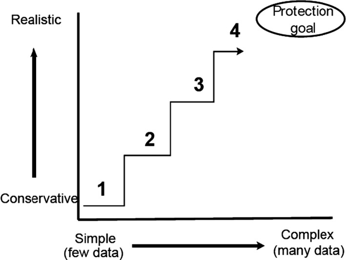
Tiers in the risk assessment process, showing the refinement of the process through the acquisition of additional data (redrafted after Solomon et al., 2008a,b)
7.3. Tiered approach in the risk assessment for amphibians and reptiles and definition of (surrogate) reference tier
A tiered approach implies the existence of a surrogate reference tier (SRT), which is a representation, as accurate as possible, of the real situation in the field (i.e. the reference tier). This SRT should link the assessment being performed and the specific protection goals (see Figure 17). A SRT is a compromise between what would be desirable and what is practical. The SRT should be used to calibrate the lower tiers properly in order to make them sufficiently protective, taking into account the level of protection defined in the SPGs.
Figure 17.
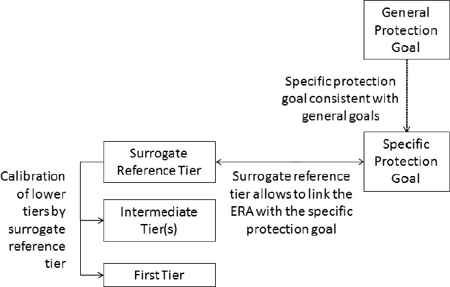
Illustration of the relationship between tiers of the risk‐assessment process and protection goals, in the approach used by the PPR Panel (EFSA PPR Panel, 2010)
Once the protection goal is clear, the tiered risk‐assessment procedure should be designed in order to evaluate whether the protection goal will be met after introduction of the active substance or PPP on the market. Such a tiered risk‐assessment procedure can be represented as a flow chart and consists of an effect flow chart coupled to an exposure flow chart. In the effect or exposure flow chart, it is always possible to jump to a higher tier, as explained in Figure 18. Each step of the effect flow chart needs an estimate of field‐exposure concentrations for the risk assessment. The ‘criss‐cross’ model (Figure 18) shows the recommended and generally accepted way of linking an estimate of the field exposure to the effect assessment: all field‐exposure tiers may be linked to any effect assessment tier, so there are no restrictions. This ‘criss‐cross’ model has the advantage of cost‐effectiveness in the risk‐assessment procedure, because changes in elements of the exposure flow chart have no consequences on changes for the effect flow chart. Thus, its modular approach enables the selection of the most cost‐effective tiers.
Figure 18.
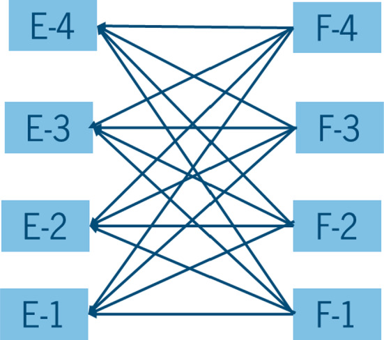
The ‘criss‐cross’ model: Tiered effect and exposure flow charts for a risk assessment addressing a specific protection goal. The boxes E‐1 to E‐4 are four effect tiers and the boxes F‐1 to F‐4 are four tiers for assessment of exposure in the field (‘F’ for ‘field’). Increasing numbers (1 to 4) indicate a higher tier that can be accessed. Arrows from right to left indicate delivery of field‐exposure estimates to the indicated effect tiers
In the tiered approach, the highest tier represents best the conditions in the field, the SRT of Figure 19 for the ecotoxicological effect assessment as well as for the exposure assessment.
Figure 19.
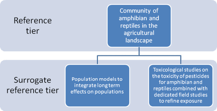
Reference tier (RT) vs surrogate reference tier (SRT) in the risk assessment of amphibians and reptiles
Regarding the highest exposure tier, it represents best all relevant entry routes of pesticides (e.g. mass deposition, crop interception and wash‐off, surface runoff) and pesticide processes (e.g. volatilisation, degradation, sorption) and generally calculates the exposure as a function of time. It is also, however, the most complex one, needing much effort. Lower tiers are less realistic, easier to apply and result in a worst‐case exposure. Coupled to an effect assessment, and calibrated to the higher tier, they allow assessment of risks at the lowest tier without too much effort. In this way, lower tiers function as a filter: if such realistic, worst‐case risk assessment indicates already safe uses, the more realistic, but effort‐consuming higher tier risk assessment is not needed. For risk assessments, the exposure assessment and the effect assessment are equally important. When linking exposure to effects, the same exposure metric should be used for both field‐exposure estimates (expressed in terms of PECs) and effect estimates (expressed as regulatory acceptable concentrations, RAC or as ecotoxicological endpoint together with an acceptability criterion) (EFSA PPR Panel, 2010).
The risk assessment of PPPs for amphibians and reptiles should be performed over different spatio‐temporal scales (in‐field, boundary‐scale, off‐field, landscape level). This is in contrast to what is currently done in the risk assessment for several other non‐target organism groups, where only the in‐field – or, separately, the off‐field area – is considered.
Since an action at a distance is also expected to occur for amphibians and reptiles on a larger scale within relevant time frames (see Section 4), a landscape‐scale assessment covering multiple field scales is considered necessary.
For many amphibian and reptile species and specific for every life stage, recovery will be driven by small‐ and large‐scale migrations together with internal recovery from reproduction within the assessed local scales (in‐field or off‐field areas). The risk to amphibian and reptile key drivers (service providing units, see Section 5) should therefore be assessed at a local scale (in‐field and off‐field habitat areas), but assessment should also consider processes at the landscape scale (see Section 4). In the latter case, this would be done using spatial population modelling to take spatial dynamics at this scale into account. The actual reference tier for amphibians and reptiles (including organisms with either high or low dispersal ability) would therefore be the community of amphibians or reptiles present at the field scale (in‐field and off‐field) and influenced by temporal and spatial processes at the landscape scale.
Since no current risk assessment scheme is available, it is difficult to define the highest tier for effect assessment that might be available in future. In aquatic studies, which are relevant, e.g. for larval stages of amphibians, the highest available tier (SRT) is represented by mesocosm studies performed at local scales. In terrestrial effect assessment, dedicated field studies or terrestrial mesocosms are relevant e.g. for the refinement of some exposure parameters for bird and mammal or for assessment of the response of amphibian and reptile communities.
Amphibians and reptiles may, however, be exposed to multiple stressors due to sequential as well as simultaneous use of different pesticides and other agricultural practices, which cannot be exhaustively studied in field experiments in the long term. Therefore, a combination of assessing the effects both at the local scale – through testing the toxicity of PPPs in effect studies on e.g. aquatic communities – and at a larger scale covering field‐boundaries and adjacent off‐field areas and other field – through modelling long‐term exposure of single species populations integrating all relevant stressors – is proposed as a SRT for amphibian and reptile species to assess population‐level effects (Figure 19). A larger‐scale approach (landscape) might be needed for the majority of amphibian and reptile species with a range of movement that will be species specific compared with field size.
In this context, it can be assumed that a suitable field study or a mesocosm study (with adequate dimensions) can act as a SRT for the assessment of community effects at a field scale for some stages of amphibian and reptile species. Such studies, e.g. on aquatic stages of amphibians, might well address community composition, population dynamics, indirect effects (predation or competition effects), chronic exposure (eventually repeated exposure), interactions between and within species and exposure mimicking the actual field situation, for example, in an aquatic mesocosm. The interpretation of such effects will have to be discussed in view of a future guidance.
However, regarding adult stages of amphibian and reptile species, short‐term field effect testing is not considered to deliver accurate responses to intended uses of PPP, since (i) the test set‐ups cannot currently take behaviour of mobile species with wide population ranges into account and (ii) it is not considered valuable and of major use to contaminate whole communities of non‐target vertebrates in field situations. Field tests can deliver generic information not depending on the PPP intended to be used, e.g. regarding presence of species in habitats of interest, their behaviour or on PPP residues on their food habits.
Long‐term dynamics at a population level over one or more seasons, embracing both population growth and spatial dynamics in‐field as well as recolonisation, should be tackled by modelling approaches (combining spatial and temporal population models). The rate parameters of these processes may depend on the field size, the spatial configuration of the crop, the PPP application scenario (application in rows or over the entire area) and the existence and dimension of field boundaries and adjacent off‐field areas. In order to assess population‐level effects, models for different ecological and agricultural practice scenarios should be developed for relevant key species, with different vulnerability components, and further validated.
In all cases, when population modelling is used, the development of suitable baseline scenarios against which to evaluate the effect is critical. Depending on the SPG, however, it is not always easy to determine which baseline will provide the most sensitive outcome (see Section 4). For this reason, the Panel recommends that in all cases a representative range with several baselines should be used, from intensive agricultural systems to extensive sustainable systems, and natural conditions in case off‐field or boundary‐scale scenarios are needed. In the case of assessment of effects on a local scale, especially in order to define normal operating ranges for communities as reference tier, extensive agricultural systems with high diversity would possibly deliver the communities to be investigated with respect to the study aims.
7.4. Surrogate reference tier (SRT) and the systems approach
Current practice in the prospective assessment of risks from PPP use is to conduct the exposure and effect assessment for one PPP at a time. An important question is whether the chemical‐by‐chemical approach in the current prospective ERA for PPPs is sufficient also to prevent cumulative risks from exposure to different PPPs, as well as to predict ecological recovery. It is therefore important to take into account the impact of multiple stressors on the state of the population when assessing a particular PPP impact. Thus, a systems approach is considered appropriate by EFSA (EFSA Scientific Committee, 2016a) owing to the complexity of ecological systems and the need to evaluate direct and indirect effects and recovery in spatial and temporal dimensions. In this context, a systems approach is defined to mean taking into account the range of factors considered to potentially interact and affect the result of the risk assessment. This could include, for example, multiple applications and non‐chemical stressors as they might affect the organisms considered in the assessment. It may also include indirect effects and abiotic factors. The SRT for this type of assessment would thus be an implemented ecological model system including the important factors identified.
In many other risk assessment schemes (e.g. non‐target arthropods, aquatic systems), the systems approach has been defined as essential owing to the impacts of both spatial and temporal drivers of population change. Spatial drivers, in particular action at a distance are relevant for those groups of organisms (EFSA PPR Panel, 2015a; EFSA Scientific Committee, 2016a). The scales and rates of movements might be even larger for amphibians and reptiles than for invertebrate species; primary drivers to be considered are temporal drivers of population change, i.e. the vital rates and migrations to and from the treated fields. The measurement endpoint in focus of this type of assessment could be the long‐term PGR. Please refer to Section 4.4 for more details on relevant population‐model endpoints.
In order to adopt a systems approach and to integrate this into the risk assessment, several steps have been described as necessary:
Relevant taxa and focal cropping systems need to be identified to create relevant scenarios. These species need to cover those where population impacts and recovery can be related to the SPGs (e.g. EFSA, 2009b).
The normal operating range of relevant taxa needs to be identified (bearing in mind that this may vary in time and between different ecosystems). In the system approach, this is used to establish different baselines against which the system with the addition of the regulated pesticide can be assessed. Such baselines would need to be established for a range of scenarios needed to represent the range of conditions that the assessment should cover (e.g. low input and high input agroecosystems).
Good mechanistic effect models, which are both manageable and realistic enough, will need to be developed. Food‐web modelling is required in order to assess effects on other species in an ecological network (De Ruiter et al., 2005). The use of food‐web models for assessment would, however, require that they are predictive and that their predictive quality has been proven in independent experiments. Hence, although food‐web models are conceptually suitable and appropriate, parameterisation and uncertainty of predictions are challenges in their application in risk assessments. For community‐level assessment, recourse must therefore be made to field studies. Note also that the longer time‐frame for field‐study assessment provides the potential to detect delayed community or life‐history effects, e.g. as a result of reproductive impacts. Food‐web models may, however, play an important role in terms of understanding the case‐specific results of field studies. In contrast, population models are relatively easy to develop and require fewer case‐specific data. Hence, for assessment of long‐term impacts, the use of population models is proposed.
The models to be developed do not need to take every possible management scenario into account. In edge‐of‐field surface waters, there are typically 2–3 pesticides dominating the mixture in terms of toxic units (see e.g. Liess and Van der Ohe, 2005; Belden et al., 2007; Verro et al., 2009). Consequently, when addressing cumulative stress of pesticides in ERA, it seems cost‐effective to focus on those pesticides that dominate the exposure in terms of toxic units in the relevant medium (e.g. > 90%). It is important, however, that a range of scenarios altering potential vulnerability of populations is taken into account (e.g. highly stressed populations may be more vulnerable to further stressors).
Information on the distribution of crops in agricultural landscapes and frequently occurring pesticide combinations may be derived from existing databases (e.g. databases under the EU subsidies scheme and databases from EU pesticide usage as collected within the frame of the Sustainable Use Directive; Garthwaite et al., 2015). This information may provide important inputs for population models to evaluate effect periods and recovery times following pesticide stress in a realistic, agricultural landscape context (e.g. Focks et al., 2014).
7.5. Recovery
Recovery can be assessed at the levels of individuals, populations, communities, or functions. In broad terms, recovery can be thought of as the return of an ecological entity (e.g. structure such as abundance, or function such as an ecosystem service) to its normal operating range (sometimes referred to as baseline properties), having been perturbed outside that range by a stressor (or multiple stressors). In order to assess recovery, it is first necessary to define what the normal operating range of the ecological entity and/or process is (EFSA Scientific Committee, 2016a).
Recovery can be classified into two main types, depending upon whether it occurs in situ (internal recovery) or via dispersal (external recovery). Both types of recovery may be exhibited by the same ecological entity (e.g. at different stages in a species’ life history). However, those organisms more dependent on external recovery will require larger scales (in both time and space) to represent their systems adequately.
EFSA recommends a systems approach in the cases where recovery is assessed (EFSA Scientific Committee, 2016a). This is due to the need to consider spatial dynamics resulting in action at a distance; hence, evaluating recovery at too small a scale may result in erroneous conclusions (Topping et al., 2014). The systems‐level approach takes into account changes in time and space over a larger scale, thus subsuming recovery under the long‐term impacts on the overall system state (e.g. represented by population size). If initial effects are considered tolerable, recovery can be considered as an essential and integral dynamic of any system subject to regulated stressors, but may not need to be taken into account explicitly if long‐term system state is used for ERA.
According to EFSA Scientific Committee (2016a), in order to show that there will be actual recovery under realistic conditions of use, any experimental or modelling approach (or combination of approaches) needs to consider:
the properties of potential stressors (including the timing of applications relative to life‐history stage, the number and frequency of applications of the same PPP and the cumulative risks of exposure to multiple PPPs)
direct and indirect effects (species interactions)
the relevant taxa and their traits, e.g. related to demography, dispersal and foraging behaviour as well as adaptation to potential stressors
the specific features of the landscape, i.e. variations in land use, and the types, spatial distribution and connectivity of habitats.
The tools used to develop the systems approach are mechanistic models for prediction, experimentation, monitoring, and expert elicitation. Experimentation usually involves semi‐field and field studies, which are primarily used for evaluating community interactions, and experimentation and monitoring are employed as a reality check and to guard against unexpected effects.
There exists a number of potential modelling approaches to assess recovery (please refer to EFSA Scientific Committee, 2016a). Employing these approaches to develop systems models, however, entails a high demand for data and expert skills for both the development and validation of potential models, especially in cases where external recovery is an important part of the dynamics.
In the case of amphibians and reptiles, recovery may not be considered as an option since any impact on populations of, e.g. endangered species is unlikely to be allowed. Short‐term recovery, e.g. by local density‐dependent compensation during larval stages may still need to be considered, depending on the agreed specific protection goals.
7.6. Ecotoxicologically Relevant Exposure Quantity
EREQ was developed from the Ecotoxicologically Relevant type of Concentration (ERC, e.g. Boesten et al., 2007). The ERC is a description of the best predictor of ecotoxicological effects that has been further developed in this Opinion (based upon Arts et al., 2015) in order to fit exposure assessment in e.g. terrestrial risk assessment, where many exposure quantities (e.g. application rates) are not reported or translated in terms of concentrations. Examples of quantities are mass, length, surface area, volume etc. (Bureau International des Poids et Mesures, 1998). The more generic Ecotoxicologically Relevant Exposure Quantity was introduced to include these other quantities.
The EREQ provides the link between the exposure and the effect assessment of PPP. EREQ is not a value but a type of exposure quantity that gives the best, or appropriate, correlation with the ecotoxicological effects. An example of EREQ for tadpoles is concentration of dissolved pesticide molecules in the pond water; or for frogs hibernating in the sediment, concentration in pore water averaged over the top centimetre of sediment.
A clear definition of EREQ is important as it forms the bridge between two fields of expertise: ecotoxicology and environmental chemistry, each with their own view on exposure in the ecotoxicity tests and in the field. In order to facilitate clear communication between the two types of experts, Boesten et al. (2007) explained which aspects of the exposure metrics should be defined. First of all, the quantity (including its spatial scale) itself plus its temporal scale should be described and next, (i) its name, (ii) conceptual definition, (iii) mathematical definition and (iv) operational definition (i.e. how the quantity can be determined experimentally) should be described. The spatial scale of the EREQ is relatively straightforward, e.g. ‘in the pond water’, ‘in the top 5 cm of sediment’. The temporal scale should represent the best suited period of time for the effect assessment and is, e.g. ‘maximum in time’ or ‘maximum time‐weighted average over five days’. An example of the other aspects is (i) name: concentration of dissolved pesticide in pond water, (ii) conceptual definition: mass of dissolved pesticide per volume of pond water, (iii): mathematical definition: c = c* − sX, with c = this quantity (mg/L), c* = total concentration of pesticide in pond water (mg/L), s = concentration of suspended solids in water (kg/L) and X = content of pesticide sorbed to suspended solids (mg/kg) and (iv) operational definition: extract water with organic solvent after filtering water and measure pesticide mass in solvent. The conceptual and operational definitions are relevant for both the effects and exposure assessments, while the mathematical definition is especially relevant for the exposure calculations.
The outcome of the exposure assessment is determined by the EREQs and their temporal scales. Different EREQs plus temporal scale lead to different selected scenarios. For example, if the EREQ was the concentration of dissolved pesticide in the pond water, the worst‐case pond would have sediment with a low organic matter content. However, if the EREQ would be the total content of pesticide in the top 5 cm of sediment, the worst‐case scenario would be a pond with high organic matter sediment. So, the exposure metric may differ for SPUs of the SPGs. Examples are: mg/individual, mg/kg organic matter in sediment, mg/L, mg/m2 soil surface area.
7.7. Exposure Assessment Goals
Exposure Assessment Goals concern the estimation of the exposure to pesticides of the Service Providing Units (SPUs) of the SPG in the environment, in the vicinity of agricultural pesticide‐treated fields (represented by the right‐hand boxes marked by a capital F in Figure 18). So the EAGs indicate the spatial unit for which the exposure should be assessed. Selecting spatial units requires insight into the ecotoxicological traits and behaviour, as well as insight into the elements determining the probability of exposure. Ecotoxicological experts and environmental fate experts should therefore cooperate to select the most relevant spatial units.
In order to be able to define the EAGs, it is necessary first to define the SPGs for each of the SPUs and the way the effects are assessed for the selected SPUs (Figure 20). In the effect assessment, the type of concentration (e.g. concentration in the water, peak or time‐weighted average) that gives the best correlation to the observed ecotoxicological effects needs to be established. Only next, it is possible to design the exposure assessment goal schemes that deliver the wished EREQ.
Figure 20.
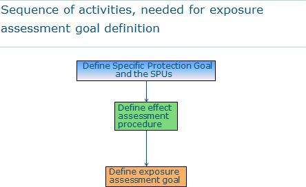
Sequence of activities to be able to define the Exposure Assessment Goal
The next example illustrates this statement. Imagine we would like to estimate the exposure in an environmental compartment, e.g. ponds where amphibians live. The exposure is via contact with pond water receiving spray‐drift deposition and pesticide‐loaded runoff. However, a contact exposure EREQ cannot be delivered, as long as it is not known what is exactly needed: e.g. which type of concentration (peak or some time‐weighted average?), when (life stage corresponding to a certain time of the year, length of exposure), or where exactly (which type or size of ponds?). So, only when the effect assessment procedure, including the SPU and EREQ, has been defined, it is possible to make a full exposure assessment, as described in an Exposure Assessment Goal Table 15.
Table 15.
Description of the elements of the exposure assessment goal linked to a certain specific protection goal for a newt species. The abbreviation ‘EA’ stands for eco(toxico)logical aspects of the SPG and ‘RM’ stands for risk managers
| Element | Explanation | Defined by | Examples |
|---|---|---|---|
| EREQ | Ecotoxicologically Relevant Exposure Quantity, i.e. key for linking with effect assessment | EA |
|
| Temporal dimension of EREQ | Determined by the requirements set by effect assessment (usually different for acute and chronic effects) | EA |
|
| Spatial unit (SU), type and size (if relevant) | Basis of SPG; link to each Service Providing Unit (SPU). Size refers to distance or area over which averaging of EREQ values is considered acceptable in view of SPG |
EA RM |
|
| Statistical population of SUs | Statistical population of spatial units considered in exposure assessment | RM |
|
| Multiyear temporal statistical population of EREQ values for one spatial unit | Based on above specifications; time series needs to be long enough to be fit for purpose | EA |
|
| Desired spatio‐temporal percentile of the statistical population of EREQ values | Determines which part of the spatio‐temporal population is excluded from the effect assessment (and may thus experience effect) |
RM EA |
|
Here, we give a schematic description of the elements used in EAGs in general terms based upon the EFSA protection goal opinion and the Guidance by EFSA SC (EFSA PPR Panel, 2010, p. 47 and EFSA Scientific Committee, 2016b). For communication purposes, we listed these elements in terms of a table (Table 15). More detailed descriptions tailored to, and in terms applicable to, the specific protection goals for amphibians and reptiles are presented in Section 6.
7.8. Linking exposure assessment to effect assessment
The risk assessment consists of two parts: (i) assessment of effects, derived from (eco)toxicological experiments (= effect assessment) and (ii) assessment of concentration levels in relevant environmental compartments or on the relevant organisms resulting from pesticide application (= exposure assessment). The EREQ has been defined as the exposure quantity that gives the best correlation to ecotoxicological effects and thus forms the interface between the effect and exposure assessments. The definition of the EREQ has allowed the tiered effect and exposure assessments to interact in a flexible and efficient way as is shown by the so‐called criss‐cross model of Boesten et al. (2007) in Figure 18.
For the risk assessment, two distinctly different exposure concentration estimates are required: the concentration related to exposure in the ecotoxicological experiments and the concentration related to exposure in the field. In the ecotoxicological experiment, assessing the exposure concentration refers to the selection of the relevant concentration to express the selected endpoint, i.e. the concentration that correlates best with the selected effect, such as mortality or reduced growth. Examples are the nominal concentration, or the time‐weighted average concentration during the initial 21 days of the experiment.
The same type of concentration should be used consistently for both types of exposure concentrations. This is represented in Figure 21 of Boesten et al. (2007), which shows the necessary activities in any combination of tiers of the effect and exposure flow charts. The four boxes drawn vertically at the left‐hand side in the effect tier box E concern the effect assessment, while the two remaining boxes concern the exposure assessment. So, both in the exposure tier F as in the effect tier E, the same type of EREQ needs to be estimated as exposure concentration.
Figure 21.
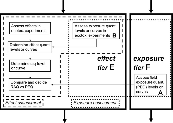
Schematic representation of activities in any combination of tiers of the effect and exposure flow chart. Note that there are two distinctly different exposure assessments in the risk‐assessment procedure, one being part of the exposure tier F that delivers field exposure and one being part of the effect tier E
In the risk assessment for regulatory purposes, decisions can be made by comparing the endpoint of the effect to the endpoint of the exposure assessment. Adjusting Boesten et al. (2007), we might use for this purpose the terms of RAQ, Regulatory Acceptable Quantity (instead of RAC, Regulatory Acceptable Concentration) and PEQ, Predicted Environmental Quantity (instead of PEC, Predicted Environmental Concentration) to encompass all exposure metrics used in both the aquatic and terrestrial environments, so not only mass per volume units, but also mass per area units or mass per mass units. This new terminology has been used in Figure 21. Note that Figure 21 illustrates the procedure not only for the aquatic environment, but also for the terrestrial environment, even if the exposure in the ecotoxicological experiment is assessed in terms of quantities per individual, e.g. mass deposited per frog.
Boesten et al. (2007) proposed to make regulatory decisions for the aquatic environment according to a tiered approach, in which RAQ and PEQ are compared according to (i) in a first step, single RAQ and PEQ levels based on conservative assumptions, (ii) in a second step, graphically RAQ and PEQ curves (describing the time courses of the RAQ and PEQ), and (iii) in a third step, time‐weighted average RAQ and PEQ levels. For the terrestrial environment this approach might be expanded to risk assessment, if the exposure in the terrestrial ecotoxicological experiment is assessed in terms of environmental concentrations or quantities, e.g. mass deposited per m2. If the exposure in the terrestrial ecotoxicological experiment is assessed in terms of quantities per individual, e.g. mass deposited per frog, the suggested tiered risk‐assessment approach needs further testing and possible development.
Other approaches with a more direct of linking exposure and effects are for example TK/TD models or landscape level approaches as explained in Section 4 could also be used to improve the linking between exposure and effects.
7.9. Combination assessment
The likelihood of showing effects depends not only on the type of active substance, the level and length of exposure, but also on other substances in the PPP and the route of entry. The later two aspects are addressed here by combination assessment.
Mixture toxicity of several substances has been addressed in previous guidance documents and scientific opinions from EFSA (EFSA, 2009b; EFSA PPR Panel, 2013, 2014, 2015a,b, 2017). The importance of addressing the effects of chemical mixtures in ecological risk assessments has, furthermore, been elaborated in a report issued by the European Commission (SCHER, SCCS, SCENIHR, 2012). In this report, a differentiation was made with regard to the relevance of mixture toxicity between the human and ecological risk assessment. For human health effects, if the intended level of protection is achieved for each individual substance, the level of concern for mixtures of dissimilarly acting substances should be assumed to be negligible. For the ecological assessment, however, population/community effects cannot be excluded based on acceptable no effect concentrations for each component. It is uncertain if the current default assessment factors are adequate to cover effects of mixtures, hence mixtures also need to be assessed for dissimilarly acting substances.
With regard to assessing the risk to amphibians and reptiles in nature, several aspects need to be considered:
Pesticidal active substances are combined with co‐formulants for optimal efficiency. It is therefore not only the active substance, but the active substance in combination with the formulation that affects target and non‐target organisms.
Amphibians may be exposed in several environmental compartments (aquatic and terrestrial) due to their mobility and biphasic life histories, and/or to mixtures within one compartment due to multiple use of different PPP in an area.
Amphibians or reptiles may be exposed via several routes within one compartment, such as oral uptake of contaminated food and dermal exposure by contact with contaminated soil.
In order to achieve the protection goals formulated for amphibians and reptiles within the context of pesticide authorisation, it is therefore relevant to consider the effects of the formulation, the exposure in different environmental compartments over the lifespan of an individual and the uptake via several routes of exposure.
7.9.1. Consideration of PPP formulations in the risk assessment
Generally speaking, co‐formulants (e.g. adjuvants) can increase the toxicity of active ingredient toxicity relative to formulation toxicity in freshwater species (Mayer and Ellersieck, 1986; Schmuck et al., 1994). With regard to amphibians, several studies have shown the impact of co‐formulants on the toxicity of active ingredients. Increased toxicity of the formulation to amphibians in comparison to the technical a.i. were reported for cycloxydim (Wagner et al., 2015), pyraclostrobin (Hooser et al., 2012), azinphosmethyl (Nebeker et al., 1998), paraquat (Linder et al., 1990) and permethrin (Boone, 2008). Furthermore different formulation types affected the toxicity of pyraclostrobin differently (Brühl et al., 2013). The most prominent and well studied example is glyphosate. In order for the anionic glyphosate to penetrate the cuticle of many plants, it is usually formulated together with surfactants such as polyethoxylated tallowamines (POEA). The addition of the POEA increases the acute and sublethal toxicity of glyphosate to amphibian larvae (Wagner et al., 2013), which is determined by the ratio of glyphosate to surfactant (Mann et al., 2009).
Knowledge about the toxicity of the active substance does not per se allow a prediction about the effect of the formulation on the toxicity. This has already been addressed in the data requirement (Commission Regulation No 284/2013), where studies with PPP are required if the effects cannot be predicted from the active substance data. Insufficient knowledge is available at present to identify formulations that increase the effects of the active substance for amphibians and reptiles. One reason is that scientists outside industry do not know the composition of the formulations.
If the toxicity of all components of the formulation is known, the toxicity can be calculated using the concentration addition (CA) approach as described in EFSA guidance documents (e.g. EFSA, 2009, 2013, see also Section 7.9.3), although there are slight differences between them (Panizzini et al., 2017). The underlying concept of CA is that the individual components of the mixture contribute to the mixture toxicity in proportion to their individual concentration and potency (Kortenkamp et al., 2009). In contrast to Directive 91/414, the current Regulation 1107/2009 requires that safeners, adjuvants and synergists should also be assessed. Potential interactions with these are not, however, routinely assessed (Panizzini et al., 2017). Whether or not the combined toxicity of the whole formulation can be addressed by the CA approach therefore depends on the available information. An experiment may often be needed to allow the required assessment of the formulation. Whether the toxicity of the formulation needs to be considered in the risk assessment needs to be evaluated when assessing the exposure.
7.9.2. Consideration of mixtures in environmental compartments
Mixture toxicity will also be of significance considering the location of shallow breeding ponds possibly in the middle of a field, where a mixture of pesticides is expected to be present. Shallow or temporary ponds may accumulate pollutants without substantial dilution (Mann et al., 2003).
Mixtures of pesticides need to be investigated in order to assess adverse impacts on amphibian development or to address the role of pesticides in amphibian declines. An increase in toxicity to Rana pipiens owing to the mixture of nine active substances at ecologically relevant concentrations (0.1 μg/L) compared with sublethal concentrations of the individual active substances was observed by Hayes et al. (2006); toxic effects included retarded and reduced larval growth, delayed development (metamorphosis) and increased disease rates, with predictable, adverse consequences for survival and reproduction. Substances (e.g. S‐metolachlor) that showed no effect on their own in the study increased the effect of other substances (e.g. atrazine), but this increased effect could be mitigated by a surfactant in a commercial mixture. Additive effects have been observed for diazinon, carbaryl, malathion and glyphosate (Relyea, 2004). Synergistic effects were observed for atrazine and chlorpyrifos in X. laevis, but not in R. calmitans (Wacksman et al., 2006). Synergistic interactions may be chemical‐specific and not ubiquitously relevant. Mixture‐toxicity assessments may be especially relevant for substances with similar modes of actions but, given the mode of action is rarely known in non‐target organisms, the combination assessment should not be limited to those.
This aspect is relevant with regard to the authorisation of products containing several active substances, but is outside the current environmental risk assessment schemes with regard to mixtures originating from the application of different products over time.
Combined exposure may also occur by moving through different compartments (either from the aquatic to the terrestrial or from field to field). The carry‐over effect from the aquatic to the terrestrial environment is not expected to occur concurrently. The biphasic life history of amphibians may, however, lead to an exposure in the terrestrial (by maternal transfer) and aquatic (by dietary of aqueous exposure) environments. This was investigated in a study with mercury, where a double jeopardy of exposure in the aquatic and terrestrial phases was identified for the American toad (Todd et al., 2011). The sequential exposure to active substances has not been investigated with amphibians yet, but was investigated with Gammarus pulex, where the order of exposure was shown to affect the toxicity due to carry‐over toxicity (Ashauer et al., 2017). The assessment of the sequential use of pesticides is not required yet, but the necessity has been identified (Verbruggen and van den Brink, 2010). A further challenge with regard to assessing the spatial‐temporal aspects is the assessment of the mixture composition in the environmental compartments as biodegradation may be affected by the mixture. Data are missing with regard to exposure of amphibians or reptiles to multiple pesticides in different compartments over their life history. The effects (e.g. interaction) of combined exposure can therefore only be addressed through a combination of experiments and models or considered in the uncertainty analysis.
7.9.3. Consideration of toxicity resulting from different routes of exposure
An individual may be exposed by a number of relevant exposure routes as described above. It is therefore considered necessary to assess the impact of pesticides on amphibians and reptiles resulting from a combination of exposure routes. A pragmatic worst‐case approach for the first‐tier risk assessment could be to combine the relevant terrestrial exposure routes by following the approach for mixture toxicity suggested in the EU guidance documents for different pesticides. The model used to estimate the toxicity of mixtures in those approaches is the assumption of dose/concentration additivity of toxicity (Loewe and Muischneck, 1926, frequently referred to as Concentration Addition (CA)) (e.g. Frische et al., 2014, Altenburger et al., 2012).
The following equation is used to derive a surrogate LC50 for the mixture of active substances with known toxicity assuming dose additivity:
| (1) |
with:
X (a.s.i) = fraction of active substance (i) in the mixture
LC50 (a.s.i) = acute toxicity value for active substance (i)
A calculated NOEC(mix) does not always constitute a reliable measure of toxicity because of (a) the dependency of NOEC values from experimental dose‐spacing, and (b) the diversity of biological endpoints in long‐term/chronic toxicity tests. Against this background, the calculated TER(mix) for a long‐term/chronic risk is only applied in the assessment in combination with additional considerations of its possible relevance in terms of actual risk.
Because of the direct proportionality of the calculated TER to the LC50 (or any other relevant toxicity value), it is also possible to calculate a TER(mix) with the following equation, often referred to Finney's equation:
| (2) |
with:
TER (a.s.i) = calculated TER for the active substance i
TER(mix) = calculated TER for the mixture
The different terrestrial exposure routes for amphibians and reptiles, such as overspray, contact with soil or plants and uptake of food, might affect the same or possibly different organs of the animal, leading to the potential accumulation of effects. It cannot be assumed per se that the effects occurring in different organs are not affecting the overall health of the organism more than by exposure to a single route. A pre‐exposure by dermal exposure may make an animal more susceptible to adverse effects if the same substance is also taken up orally. Dermal uptake by direct overspray or contact with contaminated soil may lead to local damaging effects on the skin or affect respiration, which may also be affected by inhalation.
The exposure by different routes is expressed in different units (i.e. kg/ha or mg/kg bw per day). In order to avoid the conversion of the units to internal doses for the first‐tier risk assessment, it is suggested to estimate the risk stemming from different exposure routes in a pragmatic approach using the Finney equation assuming additive toxicity. By combining the risk ratios for the different exposure routes, the units are eliminated and the relevant exposure scenarios in conjunction with possible different toxicity potentials by the different routes of exposure can be considered. An independent action in different target organs might occur, but is covered by this worst‐case approach.
The proposed risk assessment for the combination of exposure routes could be calculated as follows:
| (3) |
Or (e.g.)
1/TER(mix) = 1/TERe1 + 1/TERe2 + 1/TERe3
with:
TER(mix) = calculated TER for the combined exposure routes
TER (e i) = calculated TER for route of exposure i
e.g. e1 = oral risk quotient
e.g. e2 = dermal overspray risk quotient
e.g. e3 = dermal soil uptake risk quotient
Calculating first the risk separately for every exposure route gives the possibility to use those parameters that are relevant for the single exposure route (e.g. exposure models) and to use toxicity values (probability of effect incidence) that are typical of that route. For example, LC50 values from dermal exposure derived from direct overspray might be lower after spraying the intended rates than LC50 values for oral exposure after feeding on food items sprayed with the same dose. Each exposure route may then be refined separately prior to assessing the combined risk. TK/TD‐models may be considered relevant in a higher tier approach. The risk assessment may concentrate on a single exposure route if it clearly dominates the risk. The risk for the combined exposure is acceptable if the assessment factor for the first tier is met. If refined assessment factors are used for the different exposure routes, the approach described in the aquatic guidance document may be considered. This approach is considered suitable for the acute risk assessment of combined exposure routes as the same endpoint (mortality) is assessed. For the chronic risk assessment of combined exposure routes, the systemic effects are expected to be the same, independent of the route of exposure, but may differ in time of reaction and strength. Local effects, however, depend on the route of uptake. As described above, effects affecting different organs may decrease the overall health of the organism in combination. Uptake via different exposure routes may affect the same types of endpoints and may, therefore, also be combined for the chronic risk assessment.
7.10. The risk assessment flow chart
Amphibians and reptiles are vertebrates for which no agreed risk assessment scheme is available. There are several tests available that permit the detection of effect concentrations related to acute and chronic toxicological endpoints. Sensitive and standardised protocols are not, however, available for all life stages and exposure scenarios identified as relevant for amphibians and reptiles in agricultural landscapes (see Section 9 for further details).
Amphibians and reptiles are not only vertebrates but a group with a high proportion of endangered species (Section 2). The Panel is therefore reluctant in principle to propose dedicated toxicity studies as a standard requirement for future risk assessment schemes.
The toxicity data available are, however, scarce and a great proportion of the available information ‐ apart from studies on amphibian metamorphosis – refers to mortality or to sublethal endpoints after short‐term exposure as chosen endpoints. It might therefore be necessary, in the short‐term, to perform toxicological studies with amphibian and reptile species in order to increase mechanistic, toxicological knowledge.
The declared goal of the Panel, though, in the mid‐ and long‐term is to derive initial risk triggers to discriminate between PPP (or active substances in PPP) with potentially high or low toxicity for amphibians and reptiles; this is in order that no tests, or only a small number, will be necessary for addressing the risks for these groups in the future. The strong recommendation of the Panel is to focus scientific research on the development of combined structure–activity relationship and in vitro assays to serve in future as first steps in the assessment of risk for amphibians and reptiles. In the best case, such triggers could be derived in future also from alerts via the assessment of toxicological endpoints available for other non‐target organisms or from alternatives to in vivo testing.
The risk assessment scheme for amphibians and reptiles would in principle follow similar tiered steps as for other non‐target organisms (see Section 7.2). In a proposed risk‐assessment flow chart (see Figure 22), the evaluation of direct and indirect effects should be performed as part of the data requirements (EU 283/20135 and 284/20136, see also Section 5.1).
Figure 22.
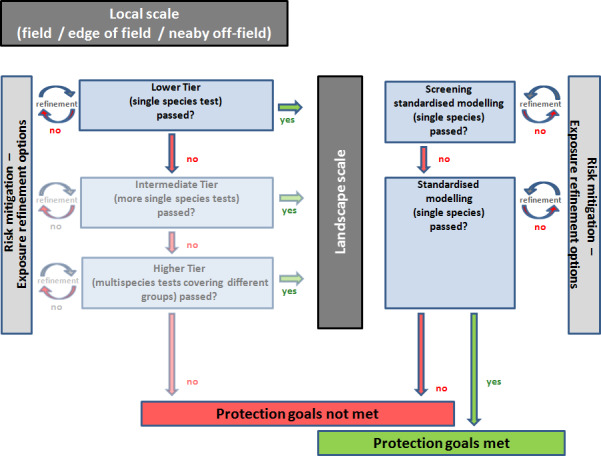
Illustrative risk‐assessment flow chart for amphibians and reptiles exposed to plant‐protection products or the active substances in PPP. In order to meet the specific protection goals for amphibians and reptiles, the criteria of both the acute and chronic effects assessment at a local scale and the long‐term population modelling at landscape‐scale components have to be passed
The proposed risk assessment scheme, as shown in the flow chart (Figure 22), has in principle subsequent components: (i) determination of acute and chronic toxicological responses for amphibian and reptile species at a local scale of assessment (ii) assessment of long‐term effects of year‐on‐year pesticide application using population modelling at a landscape scale. The principle of the scheme is that the active substance or PPP must meet acceptability criteria with respect to both components in order to decide that the protection goals for amphibians or reptiles are met.
7.10.1. Assessment of risk at the local scale
The first component of the scheme has the aim to address the acute and chronic toxicological effects of pesticides on amphibian and reptiles and to evaluate the direct and indirect impact of PPP intended uses at local scale.
The first step, as indicated in the scheme, is to investigate the acute and chronic effects of active substances or PPPs on amphibians and reptiles in simple laboratory tests. No tests have to be submitted at present according to the current data requirements (EU 283/2013 and EU 284/2013), though all available information should be delivered to authorities by the applicants.
Specific exposure scenarios and morphological characteristics of amphibians (and to a lesser extent reptiles) are not covered by the current assessment. The Panel therefore advises performing studies with a specific focus. It is proposed to characterise the toxicity of PPP (or the active substance) on developmental endpoints in chronic studies, since these might not be covered by other available data (see Section 10). It is also proposed to identify the toxicity of applied PPP on terrestrial life stages of amphibians and reptiles via dermal exposure routes, since dermal toxicity seems not to be predictable from endpoints available for other non‐target organisms (see Section 10).
Please refer to Section 7.12, and Tables 18 and 19 in Section 7.12 for a summary of the life stages considered relevant in amphibians, the acute and chronic endpoints, the coverage by available endpoints for other non‐target organisms and the conclusions for the risk assessment.
Table 18.
Amphibians, terrestrial stages. Relevant life stages, exposure routes, effects (acute here in the table means short‐term exposure and immediate effects) (chronic here in the table means long‐term exposure and also includes sublethal and delayed effects from short–term exposure), possible coverage by endpoints available for other non‐target organisms and conclusions for the risk assessment. Please refer to Sections 8, 9 and 10 in this Opinion for further details
| Life stage | Exposure route | Effects | Covered by | Conclusion | ||
|---|---|---|---|---|---|---|
| Terrestrial stages | Juvenile, adult | Contact | Over‐spray | Acute | Not covered by dermal study with birds or mammals as skin is not covered by feathers or fur and a larger part of the skin is exposed and has specific functions | New study required: overspray study (no standardised study available) |
| Chronic | Not covered by dermal study with birds or mammals as skin is not covered and a larger part of the skin is exposed and has specific functions | Not currently addressed, some conclusions can be drawn from the exposure of tadpoles followed till adult stages in the extended life cycle test based on LAGDA study | ||||
| Soil | Acute | Not covered by dermal study with birds or mammals as skin is not covered and a larger part of the skin is exposed and has specific functions | New study required if based on the overspray study the trigger is not met: exposure of adult on sprayed soil | |||
| Chronic | Not covered by dermal study with birds or mammals as skin is not covered and a larger part of the skin is exposed and has specific functions | Not currently addressed, some conclusions can be drawn from the exposure of tadpoles in the extended life cycle test based on LAGDA study | ||||
| Plants | Acute/chronic | Not covered by dermal study with birds or mammals as skin is not covered and a larger part of the skin is exposed and has specific functions | Sufficiently addressed by overspray scenario | |||
| Water puddle | Acute/chronic | Sufficiently addressed by dermal exposure route via overspray or soil | ||||
| Oral | Food | Acute | Not covered by acute oral study with birds or mammals as no correlation between toxicity could be established | Not currently addressed, no reproducible method available, considered relevant | ||
| Chronic | No data available for a comparison | Not currently addressed, no reproducible method available, considered relevant | ||||
| Inhalation | Acute/chronic | Sufficiently addressed by dermal exposure route | ||||
Table 19.
Reptiles. Relevant life stages, exposure routes, effects (acute here in the table means short‐term exposure and immediate effects) (chronic here in the table means long‐term exposure and also includes sublethal and delayed effects from short‐term exposure), possible coverage by endpoints available for other non‐target organisms and conclusions for the risk assessment
| Life stage | Exposure route | Effect | Covered by | Conclusion | ||
|---|---|---|---|---|---|---|
| Terrestrial stages | Embryo | Contact | Soil | Acute/chronic | No data available for a comparison | Not currently addressed, no reproducible method available, if data become available suggesting a need, a new method will need to be designed |
| Juvenile, adult | Water | Acute/chronic | No data available for a comparison | Not currently addressed, no reproducible method available, applies to a limited number of species/conditions. It is possible that it will be covered by a dermal toxicity test with amphibians (if developed) | ||
| Plants | Acute/chronic | No data available for a comparison | Not currently addressed, no reproducible method available, considered relevant, if data become available suggesting a need, a new method will need to be designed | |||
| Overspray (incl. stone walls, drift deposition) | Acute | No data available for a comparison | Not currently addressed, no reproducible method available, considered relevant, if data become available suggesting a need, it is possible that it will be covered by a dermal toxicity test with amphibians (if developed) | |||
| Soil | Acute/chronic | No data available for a comparison | Not currently addressed, no reproducible method available, considered relevant, if data become available suggesting a need, a new method will need to be designed | |||
| Oral | Food | Acute/chronic | Current data show poor correlation with both avian and mammalian data. | Not currently addressed, no reproducible method available, considered relevant, if data become available suggesting a need, a new method will need to be designed | ||
| Drinking water | Acute/chronic | No data available for a comparison | Sufficiently addressed by oral uptake of food | |||
Summarising the evidence for amphibians, tests in which exposure starts at the juvenile stage and is prolonged to detect the reproductive performance of amphibians after metamorphosis seem necessary in the near future (e.g. extended life cycle test based on LAGDA test, see Section 8). It should be noted that such toxicity data also deliver essential toxicity‐input parameters for long‐term modelling of populations after year on year of intended uses of PPP. Tests would also be needed in worst‐case overspray scenarios, in which the exact exposure quantities can also be determined, in order to characterise the toxicity via dermal exposure for amphibians (please refer to Section 8.3.3.)
Neither data nor test methods are available for chronic toxicity effects on reproduction of amphibians and reptiles where adult animals are exposed as in studies with bird and mammals. One possibility is to extrapolate from available test designs that assess developmental endpoints for amphibians in aquatic systems to the development of terrestrial stages of amphibians after they have left the water. The Panel is aware that long‐term exposure in both environments may not be comparable. Malformations derived from exposure in aquatic life stages (e.g. larvae) with far‐reaching consequences on adult performance could however be identified by such tests (e.g. extended life cycle test based on LAGDA test, see Section 8).
Knowledge gaps should ideally be addressed directly after being identified by this opinion, so that possibly no standard additional data will be required for performing a risk assessment according to future guidance. If, however, knowledge at time of guidance development is still lacking, then a guidance for risk assessment with specific requirements for amphibians and reptiles might be necessary. Guidance could be amended later, as understanding of toxicity mechanisms will be improved by dedicated studies. Please see the recommendation of the Panel regarding research priorities for the development of initial triggers for selective testing and alternatives to in vivo testing.
The Panel proposes for the time being that some in vivo toxicity studies with amphibians are required for upcoming assessment of active substances for approval. The basis for testing requirements is the available evidence of the impact on amphibians by intended uses of PPP that have passed the standard risk‐assessment procedures (see Section 1.4) and the legislative requirement in place (see Section 6.1).
Regarding reptiles, however, for the time being the knowledge is so scarce that the Panel cannot propose specific toxicity studies to close the data gaps. Please refer to Section 8.4 for further details and to Table 16 below.
Table 16.
Sources of uncertainty and their effects on the risk assessment for amphibians and reptiles
| Source of uncertainty in the current risk assessment | Potential to be protective | Potential to be underprotective | Impact on the risk assessment for amphibians and reptiles |
|---|---|---|---|
| Variability in toxicological sensitivity between species within one group of organisms | Variability between species is very narrow | Variability between species is very large | Variability in species unknown → further data needed |
| Representativeness in toxicological sensitivity of surrogate species for other species within one group of organisms | Surrogate species is a sensitive species | Surrogate species is not a sensitive species | Sensitivity of tested species (e.g. X. laevis) unknown → further data needed |
| Toxicological sensitivity of tested life stage | Most sensitive life stage is tested | Tested life stage does not cover sensitivity of other life stages | Sensitivity of different life stages (esp. adults) unknown, possibly compound specific (e.g. effects on eggs) → further data needed |
| Ecological relevance of observed effects in the toxicological studies | Critical effects have been addressed directly | Critical (e.g. endocrine) effects may remain unnoticed | Not all effects are adequately addressed. Sublethal studies needed to address, e.g. metamorphosis and immunosuppression |
| Study length to observe effects | Study duration long enough to observe critical and relevant effects | Study duration too short to observe latency of effects | Short‐term exposure of juveniles in the aquatic may lead to long‐term effects in terrestrial adults |
| Route of exposure addressed in the study design | Relevant route of exposure adequately addressed in the study design | Relevant route of exposure not adequately addressed in the study design | Dermal exposure currently not adequately addressed |
| Representativeness of laboratory studies and exposure models for the field | Laboratory studies and exposure models are representative for the field | Indirect effects occurring in the field are not adequately addressed in the studies. Exposure models are no representative | Extrapolation needs to be checked against field studies |
| Interaction with other non‐regulated stressors | No interactions occur | Interactions are relevant | Not addressed, e.g. Pesticide exposure may increase susceptibility to diseases |
| Multiple regulated stressors in a temporal scale (e.g. multiple applications of different products on one field) | Other products in spray schedules have no increased adverse effect | Additive or synergistic adverse effects due to treatments with several products one after the other | Not addressed. Particularly relevant for species living within the field (e.g. reptiles) or moving across the fields (e.g. amphibians) |
| Multiple regulated stressors on a spatial scale (e.g. multiple inputs in a catchment) | Habitat lies solely in field and adjacent off‐crop areas | Habitat is larger than one field, resp. receives input from several sources | Spatial scale relevant for aquatic species. Habitat range needed for terrestrial species is not addressed → further data needed |
| Location/proximity of surface water body to the field | Distance from field to water body is equal or greater than assessed | Pond may be situated in the middle of a field | Distribution of aquatic amphibian habitats needed and exposure models need to be adjusted |
| Size of standard water body (30 resp. 100 cm deep) | Depth of natural water bodies is equal or greater (90th percentile) | Habitats are very shallow temporary water bodies of a few cm depth | Description of aquatic amphibian habitats needed and exposure models need to be adjusted |
| Distribution of the test substance in test vessel to determine relevant exposure concentration | Substance is distributed in the field as in the laboratory study | Patches with increased concentration due to poor circulation in standing or slow flowing waters | Relevant exposure concentration needs to be modelled |
| Assessment of different routes of exposure separately | Exposure models are worst‐case enough so that different routes of exposure do not need to be combined | Exposure of an individual may be orally, dermally and by inhalation | Exposure models need to be adjusted to account for combined exposure routes of an individual |
| Assessment of exposure in different systems (aquatic and terrestrial) separately | Species have distinct, separate habitats | Exposure of an individual in the aquatic and terrestrial system concurrently | Exposure models need to be adjusted to account for combined exposure in water and on land |
| Health status of laboratory animals in comparison to animals in the field | Test Animal is equally healthy in the laboratory and the field | Pre‐exposure in the field increases sensitivity of the animal | Effect currently poorly understood (possibly development of resistance or increase in sensitivity) → further data needed |
| Population spatial structuring | The population exists as a spatially undifferentiated population not relying on fragile spatial dynamics for long‐term survival | The population exists as an unstable metapopulation or source‐sink population that can easily be disrupted | Not addressed. Most amphibians and many reptiles exist in spatially structured populations potentially subject to disruption |
| Long‐term year on year effects | There is no effect of previous year's impacts, i.e. full recovery within a season | There are carry‐over effects of impacts from previous years increasing the vulnerability in the following years | Not addressed. Amphibians and reptiles are long‐lived, increasing the chance of cumulative effects over a number of years building up |
Regarding the lowest tier of the proposed risk assessment scheme, test endpoints on effect of PPP on amphibians and reptiles are compared with the predicted environmental exposure quantities and then related to acceptability criteria (trigger values). For amphibian species with life stages in aquatic and terrestrial environment, assessment has to be performed both for the aquatic and for the terrestrial stages. If the acceptability criteria are met for the assessment at a local scale, then a screening of possible risks at the landscape scale is performed. The assessment can only conclude that the protection goals are met when both components of the risk assessment pass the acceptability criteria.
If the relevant trigger values are not met at the lowest tier, the risk may be refined by (i) refinement of exposure calculation (see Section 9) or/and (ii) further ecotoxicological testing (Section 8), which might improve the description of the risk for amphibians and reptiles and address specific uncertainties present at the lowest assessment steps and/or (iii) incorporation of effective risk‐mitigation options.
Intermediate effect assessment steps might address e.g. toxicity testing on more amphibian or reptile species, in order to reduce uncertainties in species sensitivity distribution. Investigation in so‐called microcosms or mesocosms with artificial species assemblages or field tests with amphibians and reptiles are possible in theory but cannot be supported as standard practice for all life stages and species. They can be used to test direct and indirect effects on species and on community composition within their appropriate scope, e.g. for aquatic life stages of amphibians with limited individual range.
Especially for adult amphibians and reptiles, no current field set‐up is available that might satisfactorily cover movements of these animals. The Panel does not, therefore, recommend further effect testing of adult amphibians and reptiles at higher tier assessment steps as standard refinement options. Suitable refinement steps are further described in Appendix J, and cover, e.g. generic field tests addressing community composition and ecological species traits. Exposure‐refinement scenarios, with the support of risk‐mitigation options, should be used as first higher tier options.
To indicate the possible lower predictive value for the field situation in addition to difficulties in the calibration of such test set‐ups with lower tiers, all intermediate and higher tier assessment steps are depicted in light grey in the assessment scheme. The Panel is aware that the uncertainties present in the different assessment steps have to be investigated and/or quantified in order to perform a proper calibration of a risk assessment scheme.
7.10.2. Assessment of risks at the landscape level
The component of the scheme addressing possible risks at the landscape level includes the descriptions of the effects of year‐on‐year application of PPPs in a so‐called ‘systems approach’ with appropriate population models (see Section 4). The assessment of long‐term effects on amphibian and reptile species is needed, since it tackles uncertainties in the risk assessment that already have to be addressed at lower tiers. Experience is still lacking in the implementation of population modelling in the risk assessment of PPP. The Panel therefore recommends further research activities in order to develop relevant population models for amphibian and reptile species and to relate model outcomes to other measurement endpoints in the risk assessment (see Section 4.2).
As defined in Section 4, one advantage of population modelling is that it takes existing toxicological response data and translates them into key, population‐level endpoints of distribution of animals in space and time and population persistence. The overall population impact is one endpoint useful for comparing changes in population size. Other endpoints addressing occupancy in addition to abundance might also prove helpful. Moreover, species abundance and occupancy can be modelled over years. The pattern of recovery of a population after PPP impact can be observed if required in population models, allowing prediction of short or long potential recovery periods after stopping PPP uses. PGR is a critical metric for population status. If PGR < 1, the population will decline and the protection goal is not sustainable.
Appropriate trigger value(s) for model output need to take into account uncertainties relating to the model, including extrapolation of population modelling results to effects at community level, as well as further uncertainties. If the trigger value(s) for model output are not met at the lowest tier, it may be possible to refine the exposure assumptions used in modelling. The results of modelling approaches assessing the effects of year‐on‐year application of PPP on amphibians and reptiles species can only be refined to a very limited extent with further ecotoxicological testing at higher tier (e.g. toxicity data for other species). Accordingly, information from higher tier tests with amphibians and reptiles (which are not recommended) will be of limited use in refining the risk indicated by population models, since these approaches are affected by different uncertainties in the risk assessment. By contrast, a monitoring programme following registration of PPP would allow for the assessment of effect predictions on populations of amphibians and reptiles.
7.10.3. Mitigation of identified risks
Although not in the remit of this Opinion, the Panel acknowledges that risk mitigation measures exist that have been implemented in practice to mitigate the risk for amphibians and reptiles after intended uses of PPP (e.g. Berger et al., 2015; Brühl et al., 2015).
Measures specifically dedicated to avoid exposure of amphibians and reptiles to PPP might include (i) the improved management of terrestrial hot spots of herpetofaunal presence, (ii) controlling PPP application on fields by time shift of application dates to reduce exposure of particular non‐target species and (iii) specifically for amphibians, measures for reducing migration demands on crop fields.
The use of PPPs should clearly follow the principles of Integrated Pest Management, being the last option after exhaustion of alternative measures. Significant numbers of amphibians and reptiles are endangered, therefore specific measures are to be taken (Art. 12 EU 2009/128) where ‘Member States shall, having due regard for the necessary hygiene and public health requirements and biodiversity, or the results of relevant risk assessments, ensure that the use of pesticides is minimised or prohibited in certain specific areas. Appropriate risk management measures shall be taken and the use of low‐risk plant protection products as defined in Regulation (EC) No 1107/2009 and biological control measures shall be considered in the first place…’
Such risk‐mitigation measures will be most effective if applied at a local level rather than at a wider regulatory level (e.g. Member State Level), since their applicability and implementation will depend on the species that are at risk in the particular environmental context as well as on the intended PPP use. A recent publication (Alix et al., 2017) addresses risk management issues to mitigate specific risks (e.g. different non‐target organisms).
As amphibian and reptile populations will be affected differently by PPP application in differently structured landscapes, effective management options at landscape scale will have to address the structure and the proportion of off‐field and/or unsprayed habitat in landscapes flagged as showing unacceptable risk. The absence of knowledge of the minimum requirements for the proportion and distribution of such features is an important data gap. It must be filled to keep exposures below critical values for intensively used and pond rich arable landscapes. (Berger et al., 2015).
Apart from the above, proven effective measures that could be considered for mitigation of identified risk at local and landscape level for targeted species are:
Enforcing unsprayed buffer strips around (as well as proper management of) breeding ponds and other suitable wet areas especially for amphibians,
provision of suitable terrestrial habitats for amphibians and reptiles
establishing flowering strips and areas in fields to reduce migration distances for amphibians
time shifting of PPP application if applicable
Possible risk mitigation measures are described in detail in Appendix K.
7.11. Addressing uncertainty in the risk assessment
Two areas where uncertainty needs to be generally addressed in the risk assessment of amphibians and reptiles are the calibration of a risk assessment scheme and the treatment of additional uncertainties in the assessment. Calibration of a risk assessment scheme is the problem (when only lower tier effects measurement data are available) when addressing uncertainty of the possible outcome of the effects‐measurement component (field or mesocosm study) of the SRT. There are likely to be additional uncertainties that need to be addressed even when highest tier effects data are available for an assessment, for example, sampling variability for a field study/mesocosm or uncertainties affecting the population modelling.
The EFSA Scientific Committee (2015) draft ‘Guidance on Uncertainty in EFSA Scientific Assessment’ provides specific guidance on the treatment of uncertainty when standardised assessment procedures are being developed. It is necessary in particular to identify and to describe all the uncertainties that affect assessments for which a standardised procedure is being developed. Methods are provided to assist with this task. The standardised procedure should include allowance for as many sources of uncertainty as is feasible. This reduces the burden for subsequent applications of the procedure as those applications need only consider uncertainties that were not already taken into account.
The outcome of a risk assessment is affected by uncertainties stemming from measurements, assumptions, extrapolations or models relied upon in the risk assessment. A certain number of uncertainties are addressed by setting an assessment factor, but further uncertainties may exist. Uncertainties may be knowledge based and can thus be quantified, reduced and potentially removed, or they may reflect the randomness of natural processes and can only be quantified (Skinner et al., 2016). The uncertainties are potentially greater for amphibians and reptiles than for surrogate species owing to the shortage of data. The question is therefore whether increasing the assessment factor can cover the uncertainties or whether new data need to be generated prior to being able to conduct a risk assessment for amphibians and reptiles. The degree of precaution decision‐makers are prepared to tolerate depends on where uncertainties reside in the risk assessment, how large they are and whether they are resolvable or not (Skinner et al., 2016). For this the uncertainties need to be located, and the sources of uncertainty and their impact on the final assessment outcome need to be identified (Draft EFSA guidance on uncertainty) in order to decide about how to proceed.
In the following Table 16, sources of uncertainties in the current risk assessment for surrogate species are identified and evaluated for their potential impact on the risk assessment for amphibians and reptiles.
For the calibration of the risk assessment scheme for amphibians and reptiles these sources of uncertainties need to be quantified. A number of uncertainties cannot be quantified at present. It is suggested that unquantified uncertainties could be combined in an increased assessment factor (draft EFSA guidance on uncertainty). It is not, however, possible to suggest an adjusted assessment factor for amphibians and reptiles to cover all uncertainties based on the currently available data and models. The Panel suggests adjusting the exposure models and gathering more toxicological data for comparison prior to deriving assessment factors.
7.12. Relevant life stages, exposure routes and effect assessment endpoints to be considered in future risk assessment
An exercise was conducted to see in how far existing developed test guidelines and study designs used in research (see Section 8 and Annex G) are suitable to address the life stages exposed via the different routes and effects on survival, development, and reproduction. Some guidelines may be expanded to address further life stages, exposure routes and effects currently not addressed, e.g. amphibian reproductive toxicity after adult oral exposure. The following test guidelines were considered as a basis to address effects in amphibians: acute fish study (OECD 203), LAGDA (Larval Growth and Development Assay) and sediment spiked tests (ASTM E2591‐07, 2013, OPPTS 850.1800, 1996).
Certainly, the challenge with regard to amphibians is the exposure via multiple routes due to their repeated aquatic and terrestrial exposure, which is not addressed with existing test guidelines. Nevertheless, rather than requesting multiple tests reflecting the complex life cycle, it is suggested to base the risk assessment on possibly two test designs i.e. a life‐cycle analysis including endpoints for reproductive toxicity (see Table 22, Section 8) and a shorter juvenile test to address the effects of dermal exposure. The derived endpoints need to be extrapolated to address multiple exposure routes. The goal at this stage is to work towards identifying substances of concern rather than assessing the relative importance of the exposure routes and/or sensitivity of every single life stage. Further research may enable a more refined effect assessment in the future.
Table 22.
Overview on amphibian test endpoints for developmental, reproductive and endocrine toxicity at different life stages. Larval stages are referred to according to the (Nieuwkoop – Faber (NF) staging system (Nieuwkoop and Faber, 1956)
| Life stage (sampled) | Endpoint measured | Endpoint for | Exposure period | Age/larval stage sampled | Test guideline | Reference |
|---|---|---|---|---|---|---|
| Embryo | Mortality | Developmental toxicity | 4 days early embryo | n.a. | FETAX | |
| Malformation | Developmental toxicity | 4 days early embryo | n.a. | FETAX | ||
| Larvae | Mortality and malformation | Developmental toxicity | From NF51 – 21 days in X. laevis, – 14 days in X. tropicalis | 7 and 21 days after NF51 in X. laevis, 5 and 14 days after NF51 in X. tropicalis | AMA | X. tropicalis: Carlsson and Norrgren (2007) |
| Growth (weight and length) | Developmental toxicity | From NF51, 21 days in X. laevis, 14 days in X. tropicalis | 7 and 21 days after NF51 in X. laevis | AMA | X. tropicalis: Carlsson and Norrgren (2007) | |
| 5 and 14 days after NF51 in X. tropicalis | ||||||
| From embryo stage NF 8 | Interim sampling at NF62 | LAGDA | ||||
| Developmental rate, developmental stage reached | Developmental toxicity | From NF51, 21 days in X. laevis, 14 days in X. tropicalis | 7 and 21 days after NF51 in X. laevis, 5 and 14 days after NF51 in X. tropicalis | AMA | X. tropicalis: Carlsson and Norrgren (2007) | |
| From embryo stage NF 8 | Interim sampling at NF62 | LAGDA | ||||
| Hindlimb length | ED mode of action; thyroid system disruption | From NF51, 21 days in X. laevis, 14 days in X. tropicalis | 7 and 21 days after NF51, in X. laevis, 5 and 14 days after NF51 in X. tropicalis | AMA | X. tropicalis: Carlsson and Norrgren (2007) | |
| Thyroid gland histology | ED mode of action; thyroid system disruption | From NF51, 21 days in X. laevis, 14 days in X. tropicalis | 21 days after NF51 in X. laevis, 14 days after NF51 in X. tropicalis | AMA | X. tropicalis: Carlsson and Norrgren (2007) | |
| From embryo stage NF 8 | Interim sampling at NF62 | LAGDA | ||||
| Juvenile | Phenotypic sex ratio | ED modes of action targeting oestrogen‐, androgen‐signalling pathways | From embryo stage NF 8 | About 2 months post‐metamorphosis in X. laevis | LAGDA | |
| Phenotypic sex ratio (gonadal histology) | ED mode of action; targeting oestrogen‐, androgen signalling pathways | Larvae | At completed metamorphosis, NF66, in Xenopus | X. laevis: Kloas et al. (1999), X. tropicalis: Pettersson and Berg (2007) | ||
| Plasma vitellogenin concentration | ED modes of action targeting oestrogen‐, androgen‐signalling pathways | From embryo stage NF 8 | About 2 months post‐metamorphosis in X. laevis | LAGDA | ||
| Larvae | At completed metamorphosis, NF66, in X. tropicalis | Brande‐Lavridsen et al. (In preparation) | ||||
| Histopathology of Müllerian and Wolffian ducts. | Potential reproductive toxicity | Larvae or juveniles | 1 month post‐metamorphosis in X. tropicalis | Jansson et al. (2016), Säfholm et al. (2016) | ||
| Gonadal maturity; oogenesis, spermatogenesis | Potential reproductive toxicity | Larvae or juveniles | 1 month post‐metamorphosis in X. tropicalis | Säfholm et al. (2016) | ||
| Adult | Calling behaviour in males | ED mode of action; targeting androgen signalling pathway | 4 days | 1–2 years in X. laevis | Behrends et al. (2010) | |
| Larynx histopathology | ED mode of action; targeting androgen signalling | Larvae | 1–2 years in X. laevis, 4–6 months in X. tropicalis | Sassoon et al. (1986), Tobias et al. (1993), Hayes et al. (2010) | ||
| Male histopathology: testis including spermatogenesis | Reproductive toxicity | Larvae or adults | 1–2 years in X. laevis, 4–6 months in X. tropicalis | Cevasco et al. (2008), Gyllenhammar et al. (2009), Hayes et al. (2010), Berger et al. (2011), Kvamryd et al. (2011) | ||
| Female histopathology: ovary including oogenesis, oviduct | Reproductive toxicity | Larvae or adults | 1–2 years in X. laevis, 6 months in X. tropicalis | Cevasco et al. (2008), Säfholm et al. (2012, 2014, 2016) | ||
| Fertility | Reproductive toxicity | Larvae or adults | 1–2 years in X. laevis, 4–6 months in X. tropicalis | Gyllenhammar et al. (2009), Hayes et al. (2010), Berger et al. (2011), Kvamryd et al. (2011) | ||
| Expression of secondary sex characters (nuptial pads, cloacal size) | ED mode of action; targeting sex hormone signalling pathways | Larvae or adults | 1–2 years in X. laevis, 4–6 months in X. tropicalis | Wyk et al. (2003), Säfholm et al. (2012) |
While it is desirable to replace the use of live animals in procedures by other methods not entailing the use of live animals, the use of live animals continues to be necessary to protect human and animal health and the environment (EU Directive 63/2010; § 10).
Table 17.
Amphibians, aquatic stages. Relevant life stages, exposure routes, effects (acute here in the table means short‐term exposure and immediate effects) (chronic here in the table means long‐term exposure and also includes sublethal and delayed effects from short‐term exposure), possible coverage by endpoints available for other non‐target organisms and conclusions for the risk assessment. Please refer to Sections 8, 9 and 10 in this Opinion for further details
| Life stage | Exposure route | Effects | Covered by | Conclusion | ||
|---|---|---|---|---|---|---|
| Aquatic stages | Egg, hatchling, larvae, metamorphic, juvenile, adult | Contact | Water | Acute | Fish acute (OECD 203) with the addition of an extrapolation factor to cover a defined percentage of amphibian sensitivity distribution (see Section 10.2) | Can be addressed with tests delivered under current data requirement |
| Chronic | Studies with surrogate species do not cover toxicity to amphibians as no correlation could be found | New reproductive study required: extended life cycle based on LAGDA | ||||
| Hatchling, larvae, metamorphic, juvenile, adult | Sediment | Acute | No study required for sediment dwelling organisms according to current data requirement | As it is not required for sediment dwelling organisms it should also not be required for amphibians | ||
| Chronic | Route of exposure covered by spiked sediment study with Chironomus sp. (OECD 218) | Not suitable to address the reproduction of amphibians | ||||
| Larvae, juvenile, adult | Oral | Food | Acute and chronic | Not covered by fish studies as uptake of food in the aquatic phase is considered to be more relevant for amphibians than for fish | Sufficiently addressed by uptake via the water phase | |
| Larvae | Sediment | Acute | No study required for sediment dwelling organisms according to current data requirement | |||
| Chronic | Route of exposure covered by spiked sediment study with Lumbriculus variegatus (OECD 225) | Not suitable to address reproduction of amphibians | ||||
For an overview on life stages, test designs and endpoints to be considered in the risk assessment see Annex G.
Figure 23.
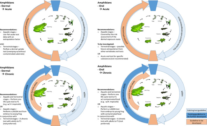
Amphibians. Overview of life stages, main exposure routes and possible recommendations for future risk assessment. Conclusions based on Table 17 and 18 above. Further details on the tests in Section 8. Discussion of coverage by tests and risk assessment performed for other non‐target organisms in Section 10. AMA: Amphibian Metamorphosis Assay; LAGDA: Larval Amphibian Growth and Development Assay
Figure 24.
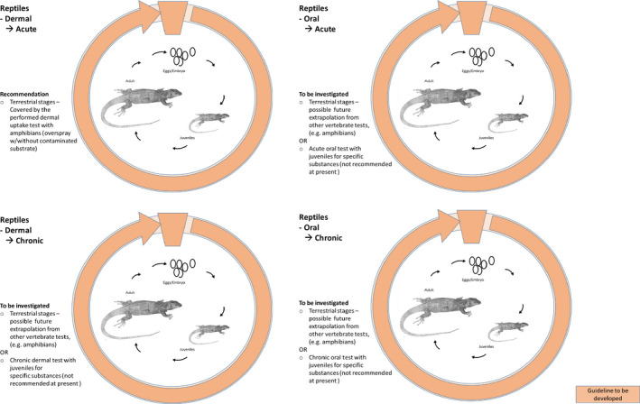
Reptiles. Overview of life stages, main exposure routes and possible recommendations for future risk assessment. Conclusions based on Table 19 above. Further details on the tests in Section 8. Discussion of coverage by tests and risk assessment performed for other non‐target organisms in Section 10
8. Toxicological endpoints and standard tests relevant for amphibians and reptiles
8.1. Introduction
Many features in the life cycles of amphibians and reptiles have been shown in laboratory experiments to be targeted by chemical exposure including embryo/larval survival, developmental rate, gonadal differentiation, spermatogenesis, oogenesis, fertility rate, and behaviour. This section is focused on test endpoints that are relevant to effects at the population level, i.e. those related to impaired survival, development, growth and reproduction, including standardised endpoints (Sections 8.1–8.4). In addition, endpoints reflective of changes in behaviour and the immune status are discussed (Section 8.5). Amphibian and reptilian model species used in toxicity studies are discussed in Section 8.6.
Lethal effects of pollutants on amphibians have been analysed in every stage of the life cycle. Information on terrestrial stages is rather limited compared with the relatively large list of papers recording embryonic or larval mortality. In toxicity tests with aquatic stages, the pollutants are usually added to the surrounding water, and the exposure route is mainly dermal but may be via gill uptake, or ingestion of substances adsorbed to food particles as well. In some studies, however, contaminated food has been used as the exposure vehicle in larvae (e.g. Cary et al., 2014). In terrestrial stages, studies recording mortality usually expose juvenile or adult individuals dermally, either through contact with contaminated surfaces (e.g. Oldham et al., 1997) or by overspray (Belden et al., 2010; Brühl et al., 2013). Recent compilations of some acute mortality data from aquatic and terrestrial amphibian stages can be found in Weltje et al. (2013) and Crane et al. (2016).
With regard to sublethal toxicity in amphibians, growth and development are the most commonly measured effects, to the point that the few standard tests available for amphibians are based on the monitoring of these endpoints (see subsection below for details of standard tests). Growth has been addressed as a response to pollutant exposure in all amphibian stages except adults. The endpoints that have been used as growth indicators are mainly body length (either total or excluding tails, if present) and body mass, although body condition has also been used as a more biologically relevant variable (e.g. Edge et al., 2011; Smith and Dibble, 2012). Growth indicators are commonly not measured at a predefined time point (e.g. after X days of exposure), but at developmental milestones such as hatching or completion of metamorphosis. There is much evidence in the amphibian biological literature that these variables at developmental milestones are important predictors of future performance of individuals (e.g. Semlitsch et al., 1988). Development is analysed in prejuvenile stages; staging systems of amphibian embryos and larvae (e.g. Gosner, 1960; Harrison, 1969; Nieuwkoop and Faber, 1994) facilitate the exposure and monitoring of developmental rates and are used systematically in studies of developmental toxicity with amphibians (Figures 25 and 26). Endpoints for other types of sublethal toxicity are presented in Sections 8.4 and 8.5.
Figure 25.
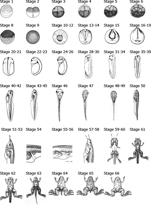
Developmental stages of Xenopus as described by Nieuwkoop and Faber (1994). The embryonic period ranges from NF stage 1–44, and the larval period from NF stage 45–65. Figure modified from Nieuwkoop and Faber (1994)
Figure 26.
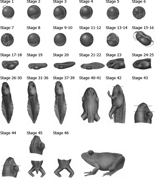
Developmental stages of Anura species according to Gosner (1960). The embryonic period ranges from stage 1–19, and the larval period encompasses stage 20–41. At stages 42–45 anurans are referred to as metamorphs. Figure modified from Gosner (1960)
The list of toxicological endpoints analysed in reptiles is much shorter than that of amphibians. As highlighted by Sparling et al. (2010), whereas amphibian ecotoxicological literature has experienced a moderate growth since the beginning of the century, reptiles continue to be an understudied group in this context and the availability of tested endpoints is extremely limited. The first consequence of the lack of ecotoxicological knowledge in reptiles is that they are the only vertebrates for which no standard tests exist.
8.2. Available standardised toxicity tests for amphibians
Two standardised amphibian test guidelines are currently available within the OECD framework: they are the Amphibian Metamorphosis Assay (AMA, OECD Test Guideline 231) and the Larval Amphibian Growth and Development Assay (LAGDA, OECD Test Guideline 241), both of which focus on the analysis of growth and developmental effects of chemicals on amphibians. In addition there is the FETAX, the Frog Embryo Teratogenesis Assay – Xenopus (Bantle et al., 1990) standardised by the American Society of Testing and Materials (ASTM test no. E1439‐12). The development of an OECD Test Guideline from a proposed new test method or from an existing standard or guideline (e.g. ASTM) involves a critical evaluation regarding its validation and regulatory acceptance. The process of test‐guideline development involves a detailed assessment of existing information; additional testing to generate new data is often needed. An interlaboratory comparative study is required when relevant (OECD, 2005).
8.2.1. The LAGDA assay
The LAGDA test design involves exposure of early life stages (embryo, larva, juvenile) of Xenopus laevis to the test substance via water (OECD 241). It is recommended to use a flow‐through exposure system and evidence should be presented to demonstrate that the concentrations of the test chemical were maintained within ± 20% of the mean measured values. The exposure is initiated at embryo stages NF 8–10 (dejellied eggs before hatching, see Table 25 for staging table) and proceeds until 10 weeks after the median time to reach NF stage 62 in the control group (about 4 months). The exposure period encompasses the sensitive windows of sex determination, gonadal differentiation and metamorphosis in X. laevis. In addition to the sampling at the end of exposure, interim subsamples are taken at NF stage 62. Endpoints in LAGDA are listed in Table 20 and include those measuring general toxicity (i.e. mortality and growth (length and weight)). In addition, endpoints indicative of specific endocrine‐toxicity modes of action (targeting oestrogen‐, androgen‐ or thyroid‐mediated physiological processes) are evaluated including histopathology of the gonads, gonad ducts, and thyroid gland (OECD 241). Hence, the LAGDA test involves an exposure period that permits measurement of endpoints both for disrupted sex differentiation and altered metamorphosis and is therefore a more complete test than AMA.
Table 25.
Elements of the exposure assessment goal for all life stages of amphibian populations (SPG: population persistence) when they are in the aquatic environment (in‐field, plus edge‐of‐field)
| Element | Description | Remarks |
|---|---|---|
| EREQ | See Table 26 | |
| Temporal dimension of EREQ | See Table 26 | |
| Spatial unit (SU), type and size (if relevant) | Ponds with surface area of 10 m2 to 2 ha | Implicitly averaging over whole surface area of pond is considered acceptable |
| Statistical population of SUs | All ponds in‐field or edge‐of‐field of treated agricultural fields in area of use of substance | |
| Multiyear temporal statistical population of EREQ values for one spatial unit | Series of tens of years of annual maxima of time‐weighted average concentration in pond water in years of treatment | Consider only concentration durations and periods that are relevant, i.e. for AMA (21 days) and LAGDA (NF 8–10 up to 10 weeks after NF 62, i.e. approximately 4 months) in their relevant periods (spring/early summer) |
| Desired spatio‐temporal percentile of the statistical population of EREQ values | Overall 90th percentile of the statistical population of each EREQ | Percentile can easily be changed if needed |
Table 20.
Endpoints, observation‐ and sampling time points in the Larval Amphibian Growth and Development Assay (LAGDA). The exposure period is initiated at embryo stages NF 8–10 and ends at 10 weeks after the median time to reach NF stage 62 in the control group
| Endpoint | Daily | Interim sampling Larvae NF62 | Test termination Juveniles 10 weeks after NF62 |
|---|---|---|---|
| Mortality and abnormalities | X | ||
| Time to NF stage 62 | X | ||
| Histo(patho)logy (thyroid gland) | X | ||
| Morphometrics (growth in weight and length) | X | X | |
| Liver‐somatic index (LSI) | X | ||
| Genetic/phenotypic sex ratios | X | ||
| Histopathology (gonads, reproductive ducts, kidney and liver) | X | ||
| Vitellogenin (VTG) (optional) | X |
8.2.2. The AMA assay
Metamorphosis is a particular feature of amphibian development. Many studies have tested disruption of metamorphosis in animals exposed to pollutants at some point during the larval period (e.g. Sparling et al., 2006a). AMA is a screening assay that was designed to identify substances that may interfere with the normal function of the hypothalamic–pituitary–thyroid (HPT) axis (OECD 231). As the components and functions of the HPT axis are highly conserved among vertebrates, AMA was suggested to represent a generalised vertebrate model. The amphibian metamorphosis is a thyroid hormone dependent process that provides the possibility to investigate whether substances interfere with the HPT axis. The general experimental design involves exposing X. laevis tadpoles for 21 days, starting at developmental NF stage 51 (see Figure 25 for staging table). The endpoints in AMA are listed in Table 21 and include hind limb length, snout‐to‐vent length (from the tip of the nose to the opening of the cloaca at the tail base), developmental stage, wet weight, thyroid histomorphometrical variables, and mortality (OECD 231). As for exposure system, a flow‐through system is preferred but in certain cases a static‐renewal system may be suitable. The concentrations of the test compound should be maintained at ≤ 20% variability of measured test concentration over the 21 day exposure period (OECD 231).
Table 21.
Endpoints and observation time points in the Amphibian Metamorphosis Assay (AMA)
| Apical endpoints | Daily | Day 7 | Day 21 |
|---|---|---|---|
| Mortality | X | ||
| Developmental stage (NF) | X | X | |
| Hind limb length | X | X | |
| Snout‐vent length | X | X | |
| Body weight (wet) | X | X | |
| Thyroid gland histology | X |
8.2.3. FETAX‐The Frog Embryo Teratogenesis Assay‐Xenopus, ASTM, E1439‐12
FETAX is a rapid (96‐h) test with Xenopus laevis to screen for acute embryo toxicity (mortality malformation, and growth inhibition). FETAX was developed to provide data on developmental toxicity for the hazard evaluation in the human risk assessment of chemicals (Bantle et al., 1999). In brief, dejellied eggs (egg from which the protective jelly layer surrounding the egg is removed) are exposed to the test compound via the surrounding water for 96 h. Mortality is recorded at the end of each 24 h period and malformations are recorded at the end of the 96‐h period. The type and degree of malformations should be evaluated against an atlas of malformations (Bantle et al., 1999). Inhibition of embryonic growth, which is the most sensitive endpoint in FETAX (Hoke and Ankley, 2005), is determined at the end of the 96 h test period by measuring head to tail length of the embryos.
8.2.4. The XETA assay (under development)
The Xenopus Embryonic Thyroid Signaling Assay (XETA) is a 3‐day thyroid disruption screening assay currently in the final phase of validation by OECD. The validation is expected to be completed by 2017 so that the test protocol may be approved as an OECD TG by 2018 at the earliest. The XETA is, like the AMA, designed to screen chemicals for potential thyroid activity.
8.3. Other test guidelines and methods used for amphibians
Apart from the two standard OECD test guidelines (LAGDA and AMA) and the widely used FETAX, some other tests have been proposed or developed by different agencies or research institutions for testing toxicity of chemicals on amphibians. The ones more commonly appearing in the scientific literature are briefly described below.
8.3.1. Standard guide for conducting acute toxicity tests
Standard Guide for Conducting Acute Toxicity Tests on Test Materials with Fishes, Macroinvertebrates, and Amphibians, ASTM E729 ‐ 96( 2014 )
This standard Guide for Conducting Acute Toxicity Tests on Test Materials with Fishes, Macroinvertebrates, and Amphibians, ASTM E729‐96(2014) describes general procedures for acute toxicity (for example, lethality and immobility) testing of a test material added to dilution water, but not to food, on certain species of freshwater and saltwater fishes, macroinvertebrates, and amphibians during 2‐ to 8‐day exposures, depending on the species. The guide describes three basic exposure techniques: static, renewal, and flow‐through and other aspects of aquatic acute toxicity testing.
8.3.2. Guidelines to conduct tests with exposure via sediment
Standard Guide for Conducting Whole Sediment Toxicity Tests with Amphibians, ASTM E2591‐07( 2013 )
This guide covers procedures for obtaining laboratory data on the toxicity of test material (e.g. sediment or soil) to amphibians. Test duration is 10 days and the overlying water may be continuously replaced or static replacement is done. The test procedure describes the use of larvae of the northern leopard frog (Lithobates pipiens). Other anuran species (for example, the green frog (Lithobates clamitans), the wood frog (Lithobates sylvaticus), the American toad (Anaxyrus americanus)) may be used if sufficient data on handling, feeding and sensitivity are available. Test material may be sediments or hydric soil collected from the field or spiked with compounds in the laboratory. Sediment toxicity testing with X. laevis has focused on evaluating the developmental effects of sediment extracts, as opposed to whole sediments, on frog embryos using the FETAX, ASTM, E1439‐12.
EPA Tadpole/sediment subchronic toxicity test OPPTS 850.1800 (1996) (USEPA, 1996 )
This guideline is used to develop data on the subchronic toxicity of chemicals sorbed to natural sediments to bullfrog tadpoles (Lithobates catesbeianus). Test duration is 30 days and is performed under flow‐through conditions. Tadpoles are exposed via spiked sediment of three different natural sediments. Exposure is by ingestion, either by direct dosage of spiked slurry into their buccal cavity at the beginning of the test in test chambers with only clean dilution water or by allowing tadpoles to ingest contaminated sediment ad libitum. Survival, growth and in addition abnormal behaviour are recorded and evaluated and LC50, EC50, LOEC and NOEC values are calculated at days 10, 20 and 30.
8.3.3. Other proposed test methods
Apart from the tests described above, some other tests have been proposed or developed by different agencies or research institutions for testing toxicity of chemicals on amphibians. The ones more commonly appearing in the scientific literature are briefly described below.
AMPHITOX: A Customized Set of Toxicity Tests Employing Amphibian Embryos
AMPHITOX is a set of acute toxicity tests on amphibian embryos reported at an ASTM Symposium by Herkovits and Pérez‐Coll (2003). To our knowledge, the AMPHITOX protocol(s) has not been published as an ASTM Standard Guide. AMPHITOX can be customised to acute (AMPHIACUT), short‐term chronic (AMPHISHORT), and chronic (AMPHICHRO) exposure periods. The main endpoint is mortality but malformations can also be recorded and the exposure periods range from 24 h up to 14 days.
The Xenopus tropicalis test system for developmental and reproductive toxicity
Chemical exposure during the development of the reproductive system in amphibians may lead to permanently impaired fertility (Gyllenhammar et al., 2009). Adverse developmental effects on reproductive function may not be detectable in the early life stages when the reproductive organs are immature (Berger et al., 2011; Kvamryd et al., 2011). It is therefore important to evaluate long‐term consequences of early life‐stage exposure to chemicals. The aquatic African clawed frog X. tropicalis has several characteristics that facilitate such studies, including a short generation time (4–6 months) compared with X. laevis (12–24 months) (Hirsch et al., 2002; Olmstead et al., 2009) and the wild European amphibian species (up to 36 months). X. tropicalis has therefore proven useful when investigating developmental reproductive toxicity, which requires life‐cycle studies (Pettersson et al., 2006; Gyllenhammar et al., 2009; Berger et al., 2011; Kvamryd et al., 2011; Porter et al., 2011). A Xenopus tropicalis life‐cycle assay has been proposed, including study design, exposure regime, and endpoints for chemical disruption of sex differentiation, reproductive organ development, the thyroxin‐regulated metamorphosis, and fertility (Berg, 2012). In addition, Xenopus tropicalis has been used to investigate reproductive toxicity after adult exposure (2–4 weeks) (Säfholm et al., 2012, 2014).
Laboratory tests to address dermal toxicity of chemicals in the terrestrial environment
All the test methods described above refer to amphibian aquatic stages, which is why the majority of ecotoxicological studies conducted on amphibians have been performed with aquatic stages. The number of assays carried out on the terrestrial phase is comparatively scarce, as is the number of studies focused on reptiles. Relyea (2005b) used a methodology to test acute toxicity of chemicals on terrestrial juvenile amphibians after overspray, a methodology that was further repeated with different chemical substances and amphibian species (e.g. Dinehart et al., 2009; Belden et al., 2010; Brühl et al., 2013; Cusaac et al., 2016), and that has also been used by industry in assessment dossiers (unpublished data). The test consists of housing animals in a terrarium and applying the chemical onto the terrarium at a realistic rate with a device simulating a professional pesticide application. The approach simulates a real scenario if it is assumed that animals are in field at the same time as pesticide applications; this scenario can be refined when the chances of animals being active at the same time of pesticide application are low (e.g. animals with nocturnal activity). In those cases, dermal exposure by contact with the applied soil may be considered, using a methodology similar to that for overspray but adjusting the application rate to expected degradation happening from real application to passage of animals over the treated soil, and introducing the animals in terraria after soil application. Likewise, crop interception can be considered by adjusting the application rate, or by including the vegetation in the terrestrial enclosure to simulate a real interception by plants (Carpenter et al., 2016). Increased realism of the exposure scenario in this type of tests can be achieved by keeping animals in enclosures in crop fields while these are being treated with pesticides (Edge et al., 2011; Cusaac et al., 2015). These types of studies maximise the realism of the exposure concentrations by intrinsically considering crop interception or pesticide drifts instead of estimating them, but on the other hand add a series of uncontrolled factors to the assays, such as environmental conditions, food availability or stress due to close presence of predators.
Mesocosm test to evaluate effects of chemicals on amphibians
Mesocosm experiments have been conducted on amphibians and reptiles and could serve as higher tier studies to evaluate the effects of pesticides or other chemicals on these animals. Studies for regulatory purposes on amphibians and reptiles have, however, not been required to date, which means that mesocosm studies conducted on these animals have not necessarily had the same purpose and design as mesocosm studies conducted for regulatory purposes on other taxa. Mesocosms for ecotoxicological studies have been used much more frequently in amphibians than in reptiles, especially for amphibian aquatic stages. Most of the mesocosm studies focusing on the effects of environmental pollutants on amphibians are designed with the purpose of evaluating such effects in an ecological context, which makes it impossible to differentiate direct toxicity caused by the chemical from indirect effects. These mesocosms often include, besides the chemical exposure, the presence of competitors, predators or pathogens; the response variables can be simply individual abundance after a given time, without the possibility of elucidating whether casualties are because of direct intoxication, predation, lack of food, disease or, most likely, a combination of several of these factors (e.g. Boone and James, 2003; Relyea, 2006). The simulation of more or less complex ecological communities sometimes results in positive, indirect effects of pollutants on amphibians in the short term by means of, for example, removing predators faster than the amphibians themselves (e.g. Relyea, 2005b); in other cases, the addition of stressors other than the pesticides results in high mortality rates of tadpoles at concentrations that are sublethal in the laboratory (e.g. Relyea and Diecks, 2008). It must be noticed as well that results from mesocosm experiments can be dependent on the set‐up conditions; for instance, Stoler and Relyea (2011) demonstrated the influence of the leaf litter mixtures used in mesocosms on all groups of aquatic communities, including amphibians. Thus, whether conditions for the studied population established at the beginning of the tests are optimal or suboptimal might influence the impacts associated with other stressors in the mesocosms, including pesticides.
8.4. Toxicity testing on reptiles
As previously established, there is a great paucity of reptile toxicity data available. The general lack of reptile acute toxicity experiments has resulted in relatively little advancement of a standardised method for reptiles. There are many barriers to the creation of a standardised toxicity test with reptiles including: (1) a general lack of either cheap commercially available species or uncertainty associated with field‐collected organisms, (2) difficulty in establishing methods for long‐term culturing of reptilian species in the lab and (3) difficulties in determining an adequate model species to represent the reptilian phylogenetic tree. There is the further consideration of reduction of vertebrate organisms used in toxicity testing from an animal welfare perspective. However, it may be important to establish standardised methods when direct testing of a reptilian species is deemed necessary during the course of a risk assessment. Furthermore, the lack of reptilian toxicity data combined with the diverse life‐history strategy has made the identification of an adequate surrogate in the traditional risk assessment paradigm challenging.
Reptiles are an extremely diverse group whose members can have very different life‐history strategies. Section 2.3 summarises aspects of reptilian biology relevant to toxicology and risk assessment. The great diversity in form and function makes it very difficult to identify specific exposure routes and life‐history stages on which to focus experiments. Table 4 of this opinion provides an overview of important exposure routes in reptiles. The lack of reptile investigations limits confidence in understanding of the relative importance of oral and dermal exposures, but a low metabolic demand suggests that dermal exposure may be a larger portion of total exposure in reptiles as opposed to estimates for birds (e.g. Weir et al., 2010, 2014, Salice and Weir, 2011). Some routes may be eliminated from consideration; for example, it is likely that inhalation sources are of relatively low concern due to relatively low respiratory rate (Weir et al., 2016a). Dermal is also of relatively little concern for terrestrial tortoises as there is little surface area for absorption. Egg exposures are possible for many reptiles as eggs are often laid in soils and can absorb pesticides (De Solla and Martin, 2011).
Much of the previous acute toxicity research has focused on squamate reptiles, specifically lizards (Weir et al., 2010). Some of the earliest dosing studies on reptiles used the green anole (Anolis carolinensis) and authors were quick to point out the lack of acute toxicity data in reptiles (Hall and Clark Jr, 1982). Very little progress was made regarding reptile toxicity methods until the efforts of Talent et al. (2002) to establish the western fence lizard (Sceloporus occidentalis) as a viable model species for laboratory testing on reptiles. The rearing of western fence lizards continued for many years and contributed to a large portion of the acute toxicity data for reptiles (e.g., McFarland et al., 2008, 2009; Suski et al., 2008; Salice et al., 2009; Weir et al., 2015, 2016b). Throughout this period, there has been an effort to improve the dosing methods of fence lizards continuing the goal of a standardised toxicity test for reptiles (Suski et al., 2008; Salice et al., 2009; Weir et al., 2015). Specific methods have been developed for acute and chronic toxicity with reptiles (Suski et al., 2008; Salice et al., 2009) as well as oral dosing methods (Suski et al., 2008; Weir et al., 2015). More recent efforts in Europe and Asia have focused on lacertid lizards as model organisms (e.g., Amaral et al., 2012a,b,c; Cardone, 2015; Chen et al., 2016), although the development of a lacertid model species for laboratory rearing has not been fully developed. Many of the European papers used field collected organisms (e.g. Amaral et al., 2012a,b; Cardone, 2015) while Chen et al. (2016) purchased their lizards from a commercially available supplier.
There have been efforts to use reptiles other than lizards as model organisms. Turtles have been used extensively in field collection methods, and have also been used in toxicity experiments in the egg (Burger, 1998; Sparling et al., 2006b) and juvenile stage (Eisenreich et al., 2009). Sparling et al. (2006b) purchased their eggs from a commercial supplier. Burger (1998) collected females from the field and induced egg laying while Eisenreich et al. (2009) collected their eggs from the field. Furthermore, a great deal of toxicity data has been developed in snakes such as the brown tree snake (Brooks et al., 1998a,b) and water snakes (e.g. Hopkins and Winne, 2006). Almost all of these studies made use of field collected organisms. A colony of breeding brown house snakes (Lamprophis fuliginosus) has been established and used in experiments related to uptake and maternal transfer of contaminants in snakes (Hopkins et al., 2004). While this model snake species has not been used in acute toxicity testing, it suggests that a standardised test with a laboratory cultured snake species is possible. Finally, crocodilians have been suggested as good model organisms specifically because they are long‐lived and have great potential for bioaccumulation of contaminants (Crain and Guillette, 1998). However, this recommendation is made more on the basis of chronic effects, endocrine disruption, etc., rather than use as an acute toxicity model organism. Crocodilians could be a good chronic toxicity subject, however, many of their life‐history strategies do not make them ideal organisms for controlled laboratory studies.
Some reptiles have life‐history strategies that make culturing and husbandry difficult. For example, some species have very long lifespans and do not reach maturity for more than a decade. This would preclude the use of these species as model species because the short turnover is not amenable to repeated toxicity testing. Additionally (and often concurrently with lifespan), some species are very large at maturity and husbandry of a functioning colony of these organisms would be difficult based on organism size. An ideal model organism would have a combination of traits that would facilitate husbandry and high productivity for repeated experiments. Talent et al. (2002) reported their efforts to find the best population of the fence lizard for creating a colony. Many populations of the fence lizard were put through a battery of tests and one particular population was found to have the highest rating on several desirable traits for a laboratory cultured organism including relatively fast growth, high fecundity and relatively young age to maturity. It is very likely that a lizard species would be the best candidate for consideration of a model organism possessing these qualities and having a relatively short lifespan and small size. Within species available in Europe, a Podarcis or Lacerta species is likely the best species for consideration for a colony used for standardised testing. The use of Sceloporus occidentalis is also an important consideration given the great effort that was previously completed to establish the fence lizard as a model species (Talent et al., 2002).
It is important to note that other vertebrate clades also contain a great deal of diversity in life‐history strategies. Some mammals (e.g. ruminants) are herbivores, while carnivora is almost exclusively carnivorous. Similar specific examples of dissimilar life histories could be found between the model organisms and the diversity of most vertebrate groups. Despite this diversity, the risk assessment process accepts the use of a few (or one) model species to represent this diversity among these clades, a similar acceptance will likely be necessary for reptiles as well.
In summary, toxicity methods for reptiles have been reported, but not formalised into a standard toxicity test. Causing further difficulty in making recommendations is the fact that the relative importance of diet and dermal exposure in relation to toxicity is not known at the moment. Therefore, it is unknown if (or to what degree) dermal toxicity and uptake need to be explicitly considered in reptile risk assessment. Future research should attempt to finalise a standard toxicity test using reptiles making an option available to risk assessors when necessary. In order to reduce the use of vertebrate species in toxicity testing, surrogacy is necessary at the screening level and immediate research needs are: (1) more estimates of acute toxicity with which to build predictive relationships between bird/mammals and reptiles and (2) more research to determine if it is necessary (and how) to estimate dermal toxicity which could then be combined with oral exposure.
8.4.1. Adapting oral avian tests
Standard oral exposure methods for reptiles should be similar to those already in place for birds and mammals. These tests could be adapted to reptiles with special considerations for dosing that have been previously investigated (Suski et al., 2008; Weir et al., 2015). Development of either acute or chronic oral exposure tests for reptiles would require the availability of a model species and potentially optimising husbandry methods to create high turnover.
8.4.2. Dermal exposure tests
The development of an amphibian dermal overspray method could potentially cover dermal exposure for reptiles. In the absence of development of such a method, a reptile‐specific method would need to be developed. Some of the methodological concerns regarding developing a dermal exposure method have been previously investigated (Weir et al., 2015). However, logistical concerns remain for developing a standardised dermal exposure method for reptiles. The procedure is similar to the one used with amphibians and consists of the application of the chemical substance to the terrarium soil before including the animals in the contaminated enclosure (Buono et al., 2007; De Falco et al., 2007). Percutaneous exposure in reptiles has been conducted most commonly by dipping parts of the animal or by pipetting the solution onto some of the animal's surfaces (e.g. Talent, 2005; Weir et al., 2015). Reptilian habits (independence from water, common use of loose soils for nesting, or frequent diurnal activity), however, make them likely to be oversprayed. Such a scenario of direct application to individuals has also been applied experimentally with similar methods to the ones described for amphibians (Carpenter et al., 2016). Although all these tests on terrestrial dermal exposure have been used mostly to test acute toxicity, the same type of experimental enclosures could be made valid for testing chronic toxicity simply by adapting exposure concentrations and experimental times. This would allow for combining dermal with oral exposure by treating food before giving it to animals, testing repeated application effects, and even analysing the effects that pollution can cause on reptilian eggs being incubated in treated soils (Rey et al., 2009).
8.4.3. In ovo toxicity testing
Currently, no standardised toxicity tests for vertebrates are available to cover potential egg exposures that occur within cultivated fields. There is not currently enough evidence to suggest that eggs are laid consistently in cultivated fields or that significant toxicity would occur from those exposures.
8.4.4. Other proposed test methods
Mesocosms for ecotoxicological studies have been used much more frequently in amphibians than in reptiles. Amaral et al. (2012d) also designed a mesocosm simulating a complex community scenario to evaluate pesticide effects on lizards, but the usefulness of their design still needs to be confirmed as the attempt resulted in high control mortality. The complexity of the mesocosm designs available in the scientific literature renders them unsuitable for testing direct toxicity and standardising their use for regulatory purposes. These mesocosm designs could serve as a starting point to set up higher tier studies adapted to environmental risk assessment of pesticides for amphibians or reptiles in case this became necessary, although this is not recommended by the Panel at present.
8.5. Endpoints for reproductive and endocrine toxicity in amphibians and reptiles
Reproductive toxicity is defined as impaired sexual function or fertility in adult individuals, and includes developmental toxicity in the offspring. Endpoints in reproductive toxicity tests include impaired fertility and reproductive organ changes in the parents as well as effects on viability, sex ratio and growth in the offspring. Reproductive toxicity such as impaired egg/sperm production can result from exposure of the adult individual as well as from exposure at early life, prejuvenile stages. The final maturation of the egg and sperm occurs in adults but the development of sperm/egg starts very early in life (during the larval stages for amphibians, in ovo for reptiles) and may consequently be damaged by chemical exposure in early life stages. Given that the critical period of sex differentiation coincides with the aquatic larval phase in most amphibians, disruption of sex‐organ development is an important endpoint for reproductive toxicity following larval exposure to water‐borne pollutants. Amphibian test endpoints for developmental and reproductive as well as for endocrine disruption are listed in Table 22.
8.5.1. Sex ratio change and ovotestis frequency
Amphibians
Alteration of the sex ratio (implying complete or partial sex reversal) relative to the control group is a commonly used endpoint for endocrine disruption in laboratory studies in X. laevis, X. tropicalis and several species of ranids including Lithobates pipens, Lithobates sylvaticus and R. temporaria (Kloas et al., 1999; Hayes et al., 2002; Mackenzie et al., 2003; Pettersson and Berg, 2007). Exposure of X. laevis larvae to the herbicide atrazine (2.5 μg/L) caused demasculinisation of the testes (Hayes et al., 2002). Mackenzie et al. (2003) investigated effects of larval exposure to oestrogenic and anti‐oestrogenic compounds (μg/L concentrations) on gonadal differentiation in leopard frogs (L. pipiens) and wood frogs (L. sylvaticus). Exposure to the test substances induced alterations of gonadal differentiation in both species. Comparisons between the two species indicated that L. pipiens is more susceptible to sex reversal and development of intersex gonads.
Oestrogen‐induced sex‐reversal during early life stages has been shown to persist long after exposure discontinued in X. tropicalis, R. temporaria and L. pipiens (Pettersson et al., 2006; Pettersson and Berg, 2007; Hogan et al., 2008; Gyllenhammar et al., 2009). Exposure of X. tropicalis larvae to environmentally realistic oestrogen (ethynylestradiol, EE2) concentrations induced female‐biased sex ratios that persisted in the adult animals, 9 months after the exposure period was ended (Pettersson et al., 2006; Gyllenhammar et al., 2009). Exposure of R. temporaria and L. pipiens larvae to EE2 induced female‐biased sex ratios that could be observed a few months after the exposure was discontinued (Pettersson and Berg, 2007; Hogan et al., 2008).
Disrupted gonadal differentiation is also an effect of antithyroid substances. Exposure of X. laevis larvae to thiourea, a thyroid hormone synthesis inhibitor, completely prevented testes formation, producing 100% females (Hayes, 1998). Exposure of X. laevis tadpoles to another antithyroid substance, ammonium perchlorate (59 μg/L), resulted in a skewed sex ratio (female‐biased) compared with the control group, suggesting that testicular development was inhibited (Goleman et al., 2002). However, in other frog species (Hyperolius viridiflavus), inhibition of thyroid hormone synthesis prevented ovary development.
The most frequently studied endpoint for endocrine disruption in wild amphibians is male intersex or ovotestis, i.e. the presence of ovarian follicles within the testicle. High incidences of ovotestis in male amphibians inhabiting agricultural areas have been reported (Hayes et al., 2003; McCoy et al., 2008). In some species, however, intersex gonads occur normally during the period of gonadal differentiation. In such species, the intersex frequency is age specific and therefore a poor indicator of endocrine disruption. Moreover, the timing of oestrogen exposure determines the extent of sex‐reversal of the testis in Xenopus laevis tadpoles (Chang and Witschi, 1956; Villapando and Merchant‐Larios, 1990). When exposure initiates at stage 44–50, all tadpoles develop ovaries whereas if exposure starts at stage 51–54, 50% of the tadpoles have ovaries and 50% have ovotestes. When oestradiol exposure started later, at stage 55–56, the gonadal sex ratio was not affected compared with the control group (Villapando and Merchant‐Larios, 1990).
Reptiles
Studies on oviparous reptiles, e.g. alligators, have been important in advancing knowledge of reptilian ecotoxicology in the field. Guillette et al. investigated the effect of estradiol treatment on gonadal differentiation in the alligator (Alligator mississippiensis), which has temperature‐dependent sex differentiation (Crain et al., 1999). Exposure of alligator eggs to estradiol induces development of females at a male‐producing temperature. Histological analysis of the gonads of female hatchlings showed that estradiol exposure increased the ovarian medullary regression (Crain et al., 1999). Another study in alligators showed that in ovo exposure to the antiandrogenic pesticide metabolite p,p′‐DDE (1,1‐dichloro‐2,2‐bis(p‐chlorophenyl) ethylene) caused a female‐biased sex ratio among hatchlings (Milnes et al., 2005).
A study on another crocodilian reptile, the broad‐snouted caiman (Caiman latirostris) investigated the effects of in ovo exposure to bisphenol A or 17β‐oestradiol on sex determination and gonadal histology (Stoker et al., 2003). The study concluded that BPA causes oestrogen‐like developmental effects by reversing gonadal sex and altering gonadal histoarchitecture (Stoker et al., 2003).
Effects of 17β‐oestradiol and the estrogenic chemical bisphenol A on sex ratio and gonadal histology were investigated in the painted turtle (Chrysemys picta), which has a temperature‐dependent sex determination (Jandegian et al., 2015). Farm‐raised turtle eggs assigned to the different exposure groups were incubated at a male‐producing temperature (26°C). Oestradiol exposure induced female gonads in 89% of the exposed ‘males’, but in none of the control males. Bisphenol A exposure resulted in the development of ovarian‐like tissue and seminiferous tubule disorganisation in the testes of hatchlings (Jandegian et al., 2015). These gonadal alterations are similar to the effects of in ovo exposure to estrogenic chemicals in birds (Berg et al., 1999, 2001a), suggesting that endocrine disrupting chemicals can induce similar effects on gonadal differentiation in birds and reptiles.
8.5.2. Reproductive organ development and fertility
Amphibians
Gonadal histomorphometry including proportions of germ cell stages to determine degree of gonad maturity in juvenile X. tropicalis have been described as potential endpoints to measure effects of toxicants on gonadal development and maturation (Säfholm et al., 2016). Endpoints for developmental toxicity in the adult amphibian testis including several histomorphometrical variables have been developed for X. tropicalis and X. laevis (Gyllenhammar et al., 2009; Hayes et al., 2010; Berger et al., 2011; Kvamryd et al., 2011). The endpoints include seminiferous tubule morphometry and proportions of male germ cell stages, analysed in histological sections (Säfholm et al., 2012). A reduced amount of mature spermatozoa in the seminiferous tubule lumen and reduced fertility rate (measured as percentage fertilised eggs in mating trials) in adult male X. tropicalis was induced by exposure of larvae to environmentally realistic EE2 concentrations (Pettersson et al., 2006; Gyllenhammar et al., 2009). It has also been shown that larval exposure to the herbicide atrazine (2.5 μg/L) decreased the frequency of seminiferous tubules with mature spermatozoa in adult male Xenopus laevis (Hayes et al., 2010). By determining the proportions of various oocyte stages in histological sections from ovaries of adult female X. tropicalis, it was shown that several progestogens (levonorgestrel, norethindrone and progesterone) inhibit oogenesis in adult X. tropicalis by interrupting formation of vitellogenic oocytes, after adult exposure to environmentally relevant ng/l‐concentrations (Säfholm et al., 2012, 2014). Ovary histomorphometrical endpoints were also used to show that oogenesis was severely impaired after larval exposure to the progestagen levonorgestrel (Berger et al., 2011; Kvamryd et al., 2011).
Impaired differentiation of the Müllerian duct or of oviduct development are effects of larval exposure to EE2 or the progestin levonorgestrel observed in X. tropicalis (Pettersson et al., 2006; Gyllenhammar et al., 2009; Berger et al., 2011; Kvamryd et al., 2011). Hence, the Müllerian ducts are targeted by several kinds of endocrine‐disrupting chemicals in amphibians. Histomorphometrical measurements of the Müllerian ducts (including size and developmental stage frequencies) that may be useful as toxicological endpoints have been developed for X. tropicalis juveniles (Jansson et al., 2016; Säfholm et al., 2016).
Reptiles
Various histomorphometrical measurements in the gonads of reptiles have been used as endpoints for disrupted gondadal development. In viviparous (live‐bearing) reptilian species (comprising about 30% of the reptilian species), exposure to environmental pollutants during embryonic development may occur via the mother, via the yolk and the placenta. A study on the viviparous lizard (Niveoscincus metallicus) showed that maternal exposure to the synthetic oestrogen diethylstilbestrol (DES) disrupted gonadal development in both male and female offspring. The male offspring of DES‐exposed mothers showed seminiferous‐tubule disorganisation and a reduction of germ cells in the testes compared with those from control groups. The female offspring to DES‐exposed mothers exhibited abnormalities of ovarian structure, oocytes and follicles compared with controls (Parsley et al., 2015).
The Müllerian ducts are also targeted by estrogenic compounds in reptiles. Increased Müllerian duct epithelial cell height in female alligator hatchlings was determined after in ovo exposure to 17β‐oestradiol (Crain et al., 1999). This is similar to the effects of in ovo exposure to oestrogen in birds (Berg et al., 2001b), suggesting that endocrine‐disrupting chemicals can induce similar effects on Müllerian duct development in birds and reptiles.
8.5.3. Vitellogenin
Elevated concentration of the egg‐yolk precursor protein vitellogenin in plasma is probably the most commonly used biomarker for estrogenic action of chemicals in oviparous vertebrates (Sumpter and Jobling, 1995; Selcer and Verbanic, 2014). The synthesis and incorporation of vitellogenin into the growing oocyte are stimulated by oestrogen but the regulation of vitellogenesis involves multiple hormones. Suppressed vitellogenesis is associated with reduced egg production and therefore reproductive success, which has been demonstrated in fish (Thorpe et al., 2007). Plasma vitellogenin concentration in juvenile X. laevis is one of the endpoints in the LAGDA test (OECD 241). A method for measuring plasma vitellogenin concentration in juvenile Xenopus tropicalis has also been developed (Brande‐Lavridsen et al., In preparation).
8.5.4. Secondary sex characters
The secondary expression of sex characters depends on sex‐hormone levels and is potentially useful as a non‐invasive endpoint for endocrine disruption. The male secondary sex characters, size of forelimb and nuptial pad, are dependent on androgen and thereby properly functioning testes (Emerson et al., 1999). Both these characters are sexually dimorphic during the reproductive phase in a wide range of frog species including the aquatic tropical species X. tropicalis and terrestrial temperate species such as R. temporaria. Exposure to antiandrogens was shown to decrease nuptial pad size in adult Xenopus (Wyk et al., 2003). The nuptial pad size in adult male Xenopus laevis was reduced after larval exposure to the herbicide atrazine (2.5 μg/L) (Hayes et al., 2010). This implies that both adult and larval exposure to endocrine disruptors can affect nuptial pad display. The development of nuptial pads in adult female Xenopus tropicalis exposed to the synthetic progestogen levonorgestrel (1.2 μg/L) for four weeks indicates that this may also be used as an endpoint for endocrine disruption in female amphibians (Säfholm et al., 2012).
Cloacal enlargement is a female secondary sex character that develops at sexual maturity. Cloacal length in adult female Xenopus tropicalis was reduced after exposure to levonorgestrel (1.2 μg/L), indicating that it might be useful as a non‐invasive endpoint for endocrine disruption in amphibians (Säfholm et al., 2012).
8.5.5. Calling/sexual behaviour
The mating process can be altered if mating behaviours are affected. In this context, pollutant effects on calling behaviour have been studied through the analysis of intensity and frequency of digitally recorded calls emitted by X. laevis males (Hoffmann and Kloas, 2012a,b). This endpoint has been proposed as a non‐invasive method for assessment of antiandrogenic endocrine‐disrupting chemicals (Behrends et al., 2010).
Competitive breeding trials have been used to measure effects of toxicant exposure on mating behaviour in X. laevis and X. tropicalis. One control male and one exposed male are put together to competed for one female and frequency of successful copulations is scored. Using such competitive breeding trials, it was shown that larval exposure to the herbicide atrazine (2.5 μg/L) suppressed mating behaviour in adult male Xenopus laevis (the atrazine‐exposed males were out‐competed by control males) (Hayes et al., 2010).
8.6. Other potential endpoints for toxicity in amphibians and reptiles
8.6.1. Amphibians
A group of sublethal endpoints that could indicate potential threats at the population level are those related to the impairment of the immune function. The amphibian immune system especially that of Xenopus, has been described in detail, and it shares most of the components of the immune system of mammals. Because the immune function is formed by a number of elements often interacting among them, testing immunocompetence of the whole organism can be very complex. The most commonly used structural and functional tests in wildlife immunotoxicological studies have also been applied to amphibians. These include measurements of both constitutive (e.g. leukocyte counts or phagocytic activity) and induced (e.g. antibody synthesis or inflammatory responses) immunity (e.g. Froese et al., 2009; Cary et al., 2014). Amphibian immune function has a particular component, the skin antimicrobial peptides, that are not present in other vertebrate groups, at least with the same degree of importance (Rollins‐Smith et al., 2005). These peptides seem to be the main barrier of defence against a number of pathogens, including the deadly fungi of the genus Batrachochytrium that are behind the decline and extinction of many amphibian populations worldwide (Rollins‐Smith, 2009). Both the amount and composition of skin antimicrobial secretions have been studied in amphibians after exposure to environmental chemicals; most importantly, their efficiency in inhibiting fungal growth in vitro can be used as a direct indicator of the immunocompetence of organisms when dealing with these pathogenic fungi (Pask et al., 2013). The outcome of potential immune suppression associated with pollutant exposure has also been investigated through the direct analysis of parasitic or pathogenic loads in exposed animals (Rohr et al., 2008; Paetow et al., 2012), and even by challenging exposed animals with pathogens in laboratory studies as a measure of final effects of immune depression (Davidson et al., 2007).
Developmental abnormalities can be quantified through the direct analysis of malformed embryos or larvae (as done in FETAX and AMA, respectively), but also by means of indicators of developmental stress like fluctuating asymmetry, which in amphibians is usually recorded for paired biometrical variables (e.g. femur length, tarsus length, Zhelev et al., 2015) rather than for patterns of asymmetry in colouration or design.
There are many other ways, besides the responses derived from hormonal disruption, by which pollutants can affect the reproductive process. In species with external fertilisation, both male and female gametes are directly in contact with the environmental pollutants in the aquatic environment right before fertilisation; the variation of the fertilisation rate of ova as a function of the concentration of chemicals in the environment can therefore be analysed in laboratory studies (Ortiz‐Santaliestra, 2008). In the majority of anuran species, mating and egg laying happen in the same sequence, which complicates the establishment of tests for addressing each of these features as specific endpoints. In caudates, however, mating and egg laying are separate processes, which has allowed the design of studies in salamanders using the alteration of these specific features as toxicological endpoints. The courtship process is subject to modified patterns if at least one of the mates suffer from toxic effects of pollution; then, the entire courtship can be screened through video recordings and altered patterns can be observed by comparing exposed and non‐exposed individuals (Secondi et al., 2013). Egg‐laying behaviour is very elaborate in some newt species that protect embryos by wrapping eggs with plant leaves; this allows for easily observing alterations in contaminated environments, as the proportion of wrapped eggs can be quantified with little effort (Ortiz‐Santaliestra et al., 2007). All these alterations related to the mating, fertilisation and egg‐laying processes are not the only way by which reproduction can be affected. Mortality of pre‐adult forms, leading to reduced recruitment, or developmental effects leading to reduced embryonic and larval survival, or to a decrease in successful metamorphosis, can also reduce reproductive outcome if compensation mechanisms are not enough to overcome such losses.
Alterations of behaviour and activity are frequently studied effects of pollutants across all life stages of amphibians (except embryos), including terrestrial stages. Alteration of behaviour is usually regarded as an indicator of neurotoxicity, although the mechanisms of how the neurotoxic action of a chemical may end up in detectable behavioural effects are very variable. Alteration of reproductive behaviours has been discussed above, but there are other behavioural displays that have been studied in amphibians. Simple locomotor activity, especially swimming performance in larvae, has been tested by recording the percentage of animals moving, the time that animals move spontaneously or as a response to prodding, or even calculating the swimming speed (e.g. Brunelli et al., 2009; Denoël et al., 2013). For instance, exposure of Bufo bufo tadpoles to endosulfan at 10 and 50 μg/L (nominal) via the ambient water from shortly after hatching to completed metamorphosis resulted in altered swimming activity as soon as four days after hatching (Brunelli et al., 2009). Larval activity can be used as a way of testing antipredator escape responses in tadpoles (e.g. Ortiz‐Santaliestra et al., 2010). Prey capture and feeding behaviours can also be studied in both aquatic and terrestrial amphibians. In general, recordings of the experimental enclosures allow for determining all kind of abnormalities in the behaviour of exposed animals. The entire feeding process in juveniles or adults can be split into prey detection (i.e. the time that the animal takes to detect the prey), approach (time since detection until actual capture) and manipulation (time since capture until complete swallowing) (Burke et al., 2010), and different patterns of alteration could suggest different types of alteration at the sensory and/or neuromuscular levels. Behaviours related to movements and orientation have been experimentally studied in amphibians; in particular, the different factors governing orientation have been addressed by leaving animals in circular arenas with different availability of potential orientation sources (Phillips et al., 2010). Although the effects of pollution on orientation or homing behaviours have not been analysed, the fact that experimental studies have been designed to investigate how these specific behaviours are displayed (e.g. Diego‐Rasilla et al., 2015) provides the possibility of implementing them as endpoints in toxicological studies.
Endpoints at the suborganismal level in the amphibian ecotoxicological literature are not as common as in bird or mammal studies, although some studies have applied the best known metabolic responses from studies with other wildlife species to amphibians. These endpoints include quantification of metabolic and detoxifying enzymes (e.g. cytochrome P450, glutathione‐S‐transferase), oxidative stress biomarkers or biomarkers of exposure or effects related to specific substances, such as inhibition of cholinesterase activity (e.g. Zhang et al., 2013; Sparling et al., 2015). Indicators of genotoxicity, and especially the micronucleus test, have also been widely observed in amphibians (e.g. Pollo et al., 2016). Toxicodynamic studies that are commonly conducted with other wildlife specimens, analysing pollutant residues in different organs and tissues, also exist for amphibians, although limited to substances with certain bioaccumulation potential like metals or POPs (Huang and Karasov, 2000). Most of the currently used pesticides have never been studied in this regard in amphibians.
8.6.2. Reptiles
Apart from the data on reproductive and endocrine disruption presented above (Section 8.5), data on sublethal responses of reptiles to pollutants are very sparse. In the field of growth and developmental effects, hatching parameters after an in ovo exposure have been reported in both lizards (Marco et al., 2004) and turtles (Sparling et al., 2006b). Neuman‐Lee et al. (2014) also studied biometry of offspring after maternal exposure of snakes to atrazine and several studies have quantified body mass gain after long‐term exposures (e.g. Salice et al., 2009). Fluctuating asymmetry is regarded as a common indicator of developmental stress and has been used as a measure of stress in some toxicological studies. In contrast with amphibians, reptiles have some clearly recognisable, paired structures other than biometrical measures that can be used in quantification of fluctuating asymmetry; these include, for example, numbers of several types of scales or femoral pores (Amaral et al. 2012b, Neuman‐Lee et al., 2014).
The most widely used endpoints of sublethal effects in reptiles are those related to behaviour. With the use of video‐recordings, prey‐capture behaviour (Amaral et al. 2012a), feeding rate (Peveling and Demba, 2003; Salice et al., 2009) or sprint speed after prodding of individuals introduced in a straight track (Amaral et al., 2012a) have been recorded as behavioural indicators of pollutant exposure in lizards. As a very specific behaviour, it is worth mentioning the time to righting of turtles after being turned on their backs, which was proposed and used by Sparling et al. (2006b) as an integrating endpoint on the basis that it is a process requiring coordination, stamina, and strength.
Some suborganismal responses have also been studied using techniques including histopathological evaluations of exposed individuals (Özelmas and Akay, 1995; Neuman‐Lee et al., 2014), plasma biochemistry (Suski et al., 2008; Salice et al., 2009), oxidative stress biomarkers (Amaral et al., 2012c), detoxification and metabolic enzymes (Yawetz et al., 1983) or specific biomarkers like cholinesterase inhibition (Yawetz et al., 1983). Some studies have managed to quantify some of these biomarkers without killing the animals, which constitutes a very important step in the application of these endpoints for monitoring of wild populations (Sanchez‐Hernandez et al., 2004).
The use of more complex designs to study pollutant effects in reptiles is scarce in laboratory ecotoxicological studies. Amaral et al. (2012d) conducted a long‐term, mesocosm experiment and recorded some of the endpoints listed above, in lizards collected from the mesocosms at the end of the assay (i.e. growth, behaviour, biomarkers, histopathology). The high mortality recorded during the experiment unfortunately means that it is difficult to draw conclusions from extrapolation of laboratory‐observed effects to responses in the field. Anyway, this study showed that terrestrial mesocosms could be adapted to reptilian ecotoxicological studies.
8.7. Amphibian and reptilian model organisms for toxicity studies
Xenopus laevis (African clawed frog) is the model species originally suggested for both OECD standard tests (AMA, LAGDA) as well as for FETAX. Both the AMA and the FETAX protocols have also been applied to other amphibian species. There are many advantages to the use of Xenopus as an experimental system, including the availability of abundant, externally developing embryos. The embryo‐larval development in Xenopus has been divided into 66 discrete stages: Nieuwkoop & Faber (NF) stages 1 – 66 (Nieuwkoop and Faber, 1956) (see Table 25 for staging table). NF stage 66 is reached when the tail has completely regressed i.e. metamorphosis is completed. This staging table is very handy in toxicity studies as it enables exposure and analysis of effects at specific developmental stages. X. tropicalis (western clawed frog) has emerged as a useful model organism because of its short generation time and diploid, sequenced genome (Hirsch et al., 2002; Berg et al., 2009; Hellsten et al., 2010). The generation time of X. tropicalis is about 4–6 months compared to 12–24 months in Xenous laevis (Hirsch et al., 2002; Olmstead et al., 2009) and has therefore proven useful in life cycle studies (Pettersson et al., 2006; Gyllenhammar et al., 2009; Berger et al., 2011; Kvamryd et al., 2011; Porter et al., 2011). The use of X. tropicalis as an alternative to X. laevis as a test species in the AMA and the FEATX tests has been evaluated (Fort et al., 2004; Carlsson and Norrgren, 2007). Both studies concluded that there were no substantial differences between the species in terms of type of effects or sensitivity to the test substances evaluated, suggesting that X. tropicalis could be used effectively as an alternative test organism for the AMA and FETAX tests (Fort et al., 2004; Carlsson and Norrgren, 2007).
Prior to the year 2000, most of the reptilian ecotoxicological literature focused on the endocrine disruption of alligators living in contaminated areas of North America. Based on the knowledge accumulated, Crain and Guillette (1998), and Crews et al. (2003) proposed using reptiles as models for studying endocrine disruption. Later, Talent (2005) proposed the western fence lizard (Sceloporus occidentalis) as a model species for ecotoxicological assessment, which could lead to further implementation of standard tests using this species. Weir et al. (2015) further applied the proposed role of this species as a reptilian model in ecotoxicological and risk assessment research. Among European species, Amaral et al. (2012a, b, c, d)focused much of their work on the Bocage's lizards (Podarcis bocagei) showing the potential of this small‐sized lizard to be used as a reptilian model in laboratory studies. In general, the developmental of tests using reptiles as model species is very limited, perhaps because reptilian tests are at present not required for regulatory purposes, but already tested species like S. occidentalis or P. bocagei should be the first options to consider in case that reptilian models are necessary in future ecotoxicological standard tests.
8.7.1. Differences in susceptibility to reproductive toxicity in amphibian model species
Interspecies comparisons of susceptibility to developmental and reproductive toxicity in amphibians are difficult because of a lack of data. Most comparative studies investigate effects of EE2 a potent oestrogenic pharmaceutical and environmental pollutant, or atrazine. The susceptibility of X. tropicalis and R. temporaria to oestrogen‐induced disruption of gonadal differentiation was investigated in (Pettersson and Berg, 2007). Larvae of the two species were exposed to EE2, a potent oestrogenic pharmaceutical and environmental pollutant, from shortly after hatching until completed metamorphosis. Larval EE2 exposure caused female‐biased sex ratios at similar concentrations: 18 ng/L (0.06 nM) in X. tropicalis and 27 ng/L (0.09 nM) in R. temporaria. This study indicates that the effect of larval oestrogen exposure was similar i.e. male‐to‐female sex reversal, and that the sensitivity of the two species to EE2 with regard to this endpoint was comparable.
Tamschick et al. (2016) investigated the susceptibility of sex differentiation to oestrogen‐induced disruption in three divergent anuran families, X. laevis (Pipidae), Hyla arborea (Hylidae) and Bufotes viridis (Bufonidae). The tadpoles were exposed to EE2 at the concentrations of 0, 50, 500 and 5,000 ng/L. The lowest exposure concentration that caused gonadal effects was 500 ng/L in all three species, but the effects differed between the species i.e. gonadal sex‐reversal was shown in X. laevis and H. arborea whereas mixed‐sex (intersex) gonads was a more pronounced effect in B. viridis. Hence, the sensitivity of the three species to oestrogen‐induced gonadal effects seems comparable although the nature of the effect differed. This in turn may be due to interspecies differences in exposure period relative to the gonadal differentiation period. It has been shown in X. laevis tadpoles that the timing of oestrogen exposure determines the extent of sex‐reversal of the testis as described above (Chang and Witschi, 1956; Villapando and Merchant‐Larios, 1990).
Mackenzie et al. (2003) investigated effects of larval exposure to oestrogenic and anti‐oestrogenic compounds (μg/L concentrations) on gonadal differentiation in northern leopard frogs (L. pipiens) and wood frogs (L. sylvaticus). Exposure to the test substances induced alterations of gonadal differentiation in both species. Comparisons between the two species indicated that R. pipiens was more susceptible to sex reversal and development of intersex gonads.
Hayes et al. (2002, 2003) examined effects of atrazine on sexual development in X. laevis and L. pipiens. Larvae were exposed to atrazine (0.01–200 μg/L) by immersion throughout larval development. Atrazine exposure (≥ 0.1 μg/L) induced hermaphroditism in X. laevis males (Hayes et al, 2002). In L. pipiens atrazine exposure (≥ 0.1 μg/L) resulted in retarded gonadal development (gonadal dysgenesis) and testicular oogenesis (hermaphroditism). Hence, these studies suggest that X. laevis and L. pipiens exhibited comparable sensitivity to atrazine (Hayes et al., 2003).
8.8. Conclusions
Laboratory experiments have shown that there is a range of toxicological responses in amphibians and reptiles that are potentially useful as test endpoints for impaired embryo/larval survival, developmental rate, gonadal differentiation, spermatogenesis, oogenesis, fertility rate, and behaviour. For an overview on life stages, test designs and endpoints to be considered in the risk assessment see Annex G.
Three standardised tests are available for amphibians: LAGDA, AMA, and FETAX. Of these, LAGDA is the most extensive test with an experimental design that allows detection of disrupted metamorphosis as well as sexual development in the model species X. laevis. AMA is designed to detect effects of chemical exposure on metamorphosis but the exposure period does not encompass the sensitive windows of sex determination and gonadal differentiation in X. laevis. None of the above tests, however, covers the reproductive ability of amphibians. A full life cycle test with amphibians (e.g. with X. tropicalis, which has a shorter generation time than X. laevis) could be very useful in a risk assessment context because it enables the identification of impaired reproductive function following exposure during a sensitive window of development.
No standard test guidelines exist for reptiles and there is a lack of toxicity data for this group of vertebrates. This makes it very difficult to compare the toxicological sensitivity among different reptile species. Standard test protocols should be developed for reptiles in order to close these knowledge gaps in future.
The potential of relying on other vertebrates as surrogates for amphibians and reptiles to cover toxicity of PPPs is compromised by some particular biological processes typical of these animals, including metamorphosis in amphibians or hormone‐dependent sex determination and sex organ development in both amphibians and reptiles. Thus, impacts of pesticides need to be assessed for specific, sensitive time windows within the amphibian aquatic development. It is suggested that research is conducted to develop in vitro tests for acute and chronic effects.
9. Exposure assessment in the environment
9.1. Introduction
The ecological attributes of the specific protection goals (SPGs) have been defined for amphibians and reptiles both at the level of individuals and the population (Section 6). At an individual level, both the individual juvenile and adult amphibians and reptiles are to be protected, while at the population level, all life stages (including eggs) are potentially important. This implies that possible exposure routes during all life stages of amphibians and reptiles need to be considered.
Amphibians have an aquatic as well as terrestrial habitat, while reptiles mainly live terrestrially. Below we first consider the exposure for amphibians, both aquatic and terrestrial, and next, the exposure for reptiles. Because the SPGs concern in‐field as well as off‐field habitats, the exposure needs to be assessed in‐crop and off‐crop. In the following the different environments (aquatic, terrestrial, in‐crop, off‐crop) have been addressed separately. An individual may, however, be exposed in multiple environments throughout its lifespan. Note that the tables summarising the exposure routes in the Sections 9.2 and 9.3 have been based on expert judgement and are not rigorously based on data, as these are insufficiently available. In the following, the different routes of exposure will be addressed separately. An individual may, however, be exposed through multiple routes at the same time or also throughout its lifespan.
Tables have been drawn below for the Exposure Assessment Goals, including their specific elements, as well as the exposure routes that are coherent with the SPGs defined at the level of individuals (no mortality) for both the aquatic and terrestrial environment of amphibians and for reptiles. For population persistence, SPG tables on the Exposure Assessment Goal and exposure routes were drawn for amphibians in the aquatic environment only, based upon the two standardised amphibian test guidelines available within the OECD framework: the Amphibian Metamorphosis Assay (AMA) and the Larval and Growth Development Assay (LAGDA). The endpoints which can be derived from these tests can be used in the risk assessment. However, we here use both tests especially as examples, as other tests do not exist and thus this is the only way to demonstrate how the Exposure Assessment Goals and EREQs are linked to the effect assessment tests. The Working Group did not draw tables for Exposure Assessment Goals and exposure routes that are coherent with the SPGs of population persistence with its attributes of abundance/biomass, distribution and population growth for amphibians in the terrestrial environment and for reptiles, except for eggs in nests. At present, no detailed and quantitative definitions of the SPG population persistence for its attributes exist for EU registration, especially for amphibians in the terrestrial environment and for reptiles other than their nests; it is therefore not yet possible to define satisfactorily, e.g. the spatial unit and its statistical population. This may be possible in a later stage. Population modelling presented in Section 4 may be an alternative way to evaluate the SPGs of population persistence in the future.
9.2. Exposure of amphibians
9.2.1. Aquatic environment
The entirely aquatic life stages of amphibians are aquatic eggs, hatchlings and larvae (tadpoles). At the end of the larval stage, the larvae undergo metamorphosis and transform into terrestrial juveniles and, next, adults. Juveniles and adults also stay part of their time in the aquatic environment and some even hibernate in the sediment of water bodies. So, all life stages may be exposed to pesticides via the aquatic environment.
9.2.1.1.
Type of aquatic habitats
A variety of water body types may be the aquatic habitat of amphibians. Ponds or pools, but also ditches, canals, small and bigger streams and even (artificial) lakes may host amphibians. Ponds may be isolated, but also linked to an inflow or outflow (Figure 27). The majority of amphibians have a preference for environments without predators such as fish, so temporary ponds are preferred habitats.
Figure 27.
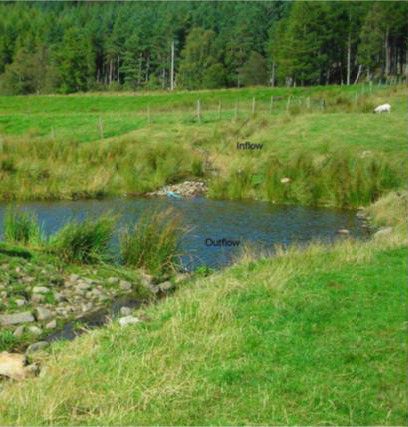
Pond having inflow and outflow in the UK (source: Williams et al., 2010)
The depth of the water bodies may be as low as a few centimetres. Permanent water bodies mostly occur off‐field, whereas temporary water bodies may occur in the middle of a treated field as well as off‐field. The formation of temporary ponds depends on the amount of rainfall and soil characteristics. They may be recharged by rainfall (southern Europe) or groundwater (northern Europe). Drainage may also recharge temporary ponds in the field (personal communication DE and CH).
There is little knowledge on the distribution of ponds where amphibians dwell (see also Appendix C on dimensions etc. of ponds in Spain, the UK and Switzerland). Surrounding agricultural land use of such ponds determines exposure concentrations, e.g. in ponds located in grassland/meadows, exposure to pesticides will be much lower than in ponds located in arable land, such as potatoes or cereals. For instance, in a country like the Netherlands more amphibian ponds can be found in habitats surrounded by grassland than in habitats surrounded by agricultural crops.
Dimensions and surrounding land use of amphibian ponds in Spain and Switzerland and ponds in the UK and comparison to water bodies of the EU FOCUS surface water scenarios
In Appendix C, the Working Group gathered data on surface area, water depth and water volume of ponds and other (mostly standing) water bodies serving as aquatic habitat for amphibians, as well as on land use in their immediate surroundings. The dimensions of amphibian ponds are important to be able to determine pesticide concentrations in the ponds. By assessing whether agricultural land use occurs in the immediate surroundings of the ponds, we are able to evaluate whether the amphibians are likely to be exposed in their aquatic habitat. In addition, the dimensions of the amphibian ponds were compared to the dimensions of the so‐called FOCUS surface water bodies (pond, ditch and stream) that are currently used in the risk assessment for the aquatic ecosystem at EU level. This was done in order to assess whether the PEC values are ‘realistic worst case’ in the FOCUS water bodies used in the regulatory process.
In Spain, 794 water bodies serving as amphibian breeding sites were monitored from 2010 onwards. The water bodies have been classified as ponds (421), artificial pool (152), dam/reservoir (66), lagoon/lake (21), river (30), stream (85) and wetland/marsh (19) (Spanish Herpetological Society, November 2016, http://siare.herpetologica.es/sare).
In 18% of the water bodies, water depth was 30 cm or less (30 cm is the minimum water depth of the FOCUS ditches and streams).
In 70% of the water bodies, water depth was 1 m or less (the depth of the standard FOCUS pond).
In 59% of the water bodies, water surface area was less than or equal to 100 m2 (the surface area of the 100 m × 1 m FOCUS ditches and streams).
In 87% of the water bodies, surface area was less than 900 m2 (the surface area of the 30 m × 30 m FOCUS ponds).
These data demonstrate that water depth and water surface area of the Spanish water bodies, serving as amphibian breeding sites, are in the same range as those of the FOCUS ditches, streams and ponds, but that the large majority of these Spanish water bodies have a smaller water depth and surface area than the FOCUS pond.
Land use data were available for 151 Spanish ponds used by amphibians. For 70 ponds, agricultural fields were present within 100 m distance, out of which 13 ponds were entirely surrounded by agricultural fields. These data demonstrate that a non‐negligible proportion of the ponds in Spain in which amphibians live, are likely to receive pesticides residues.
In the canton Aargau of Switzerland, there has been an amphibian monitoring programme since 2006 (Kanton Aargau, Abteilung Landschaft und Gewässer, Projekt Amphibienmonitoring Aargau, 2016). Eight amphibian species were surveyed. Ponds were selected based on the occurrence of one of these eight species and in total 754 water bodies are surveyed. Volunteers estimated pond surface areas during the period mid‐June to end of July (with some exceptions between March and September) but water depths were not recorded.
In 52% of the water bodies, surface area was 100 m2 or less (the area of the FOCUS ditches and streams)
In 89% of the water bodies, surface area was 900 m2 or less (the area of the FOCUS ponds).
There are no data for the Swiss canton ponds that specify the land use in their immediate surroundings. Aargau is a canton with intensive agriculture and a good distribution of amphibian populations, therefore a number of the ponds in the survey are likely to represent amphibian habitats that may receive pesticide residues.
In the UK, the current state of ponds was surveyed and described in the Countryside Survey of 2007 (Williams et al., 2010). A pond was defined as a body of standing water of 25 m2 to 2 ha, in area, which usually holds water for at least 4 months of the year. Ponds smaller than 25 m2 were not recorded, although they might have been present. The survey made an inventory of all ponds (as defined above), including ponds where amphibians may not be present. It covered a total of 591 1 × 1 km square samples spread across England, Scotland and Wales. The ponds may be isolated or not. The survey demonstrated that almost two‐thirds (63%) of ponds were directly linked to the stream network and that a third of these ponds had an inflow but no outflow, suggesting that many ponds intercept and retain drainage water. The database contained 259 ponds but water surface area was measured only for 257 ponds, mostly in the period May–October 2007.
23% of the 257 ponds with measured water surface had a surface area of 100 m2 or less (the surface area of FOCUS ditches and streams)
79% of the 257 ponds with measured water surface had a surface area of 900 m2 or less (the surface area of the FOCUS ponds).
The depth was measured for 109 ponds. The maximum depth was not measured in the remaining 150 ponds, because it was too deep to wade; thus the data on water depth are biased with maximum water depth over 1 m not represented. For 69 of the 109 ponds where depth was measured, the water depth was below 0.3 m or less, and these 69 ponds represent 27% of the total of 257 ponds.
These data demonstrate that for the majority of the 257 UK ponds the water surface area is in the same range as the FOCUS water bodies, but that in 58% (150/259) of the UK ponds the water depth is greater than the 1 m of the FOCUS pond. Note that the presence of amphibians was not confirmed in all ponds of this data set and that ponds with areas below 25 m2 (although widely present in the UK landscape) or above 2 ha were not included in the data set.
Depending on the classification of arable land use (presence in the 0–100 m perimeter around the ponds, or the regionally based land use classification of the ITE, Institute of Terrestrial Ecology) approximately 20% (59 of the 259 ponds) or nearly 50% of the ponds (115 of the 259 ponds) had significant arable land use in the vicinity of the ponds.
The presence of amphibians (e.g. tadpoles, frogs, newts) was recorded. Amphibians were observed in 49 of the 259 sampled ponds. This number is expected to be an underestimation of reality, as the observation of amphibians will depend on the expertise on amphibians of the surveyor as well as on the time of the year of the survey (often between April/May to October/November).
The analysis of the dimensions of the Spanish and Swiss amphibian ponds and the CountrySide Survey ponds in the UK and their comparison to the FOCUS surface water bodies demonstrates that the most vulnerable 10% of ponds are significantly smaller than the FOCUS ponds. Therefore, we expect the 90th percentile peak concentration to be significantly higher in the analysed ponds than in a FOCUS pond (Appendix C). This means that we expect peak concentrations in FOCUS ponds not to be conservative estimates for the exposure concentrations in the ponds in the surveys. It is more complicated to compare the peak concentrations in FOCUS ditches and streams with the ponds in the surveys, therefore the Panel was unable to make a general statement on whether or not peak concentrations in FOCUS ditches and streams are conservative for the ponds in the surveys. In view of the higher flow‐through rates in the FOCUS ditches and streams, however, the pesticide concentrations are expected to decline more rapidly in the FOCUS ditches and streams than in the ponds of the surveys and thus they probably underestimate chronic exposure in the surveyed ponds. The Panel therefore expects that the FOCUS ditches and streams are not conservative for the chronic risk assessment of exposure in ponds used by amphibians in the EU.
The Working Group compiled Annex B, which gives an overview of characteristics of ponds hosting amphibians, required to be able to make a spatio‐temporal statistical distribution of environmental concentrations across the EU. From such a distribution, ponds with the desired percentile ‘worst‐casedness’ in concentration could be selected and used to perform the amphibian risk assessment.
Surface area and water depth of ponds for amphibian species in Europe
A literature search on amphibian breeding sites resulted in the type and size of water body within Europe in which different amphibian species prefer to breed (Appendix E). In 104 publications, the size measurements of the water bodies were reported, of which 61 contained data suitable for further analysis. Data were analysed from studies where it was explicitly specified that ponds were used as breeding sites or wherever the presence of juveniles, tadpoles or eggs was reported. Surface area and water depth were determined: minimum and maximum values, as well as means and medians for various amphibian species. The surface area of breeding sites and water depth were evaluated for 17 and 16 amphibian species, respectively (Figure 28). Median surface areas ranged from 4.50 to 3,500 m2 for Discoglossus galganoi (n = 3) and Hyla meridionalis (n = 2), respectively (Garcia‐Gonzalez and Garcia‐Vazquez, 2012; Ruhi et al., 2012). The smallest median depths were reported for Discoglossus pictus (n = 10) and Epidaelea calamita (n = 14) with 0.18 m (Ruhi et al., 2012; Sebastian et al., 2015). The maximum median depth was 1.20 m, reported both for Bufo bufo (n = 6) and Pelobates fuscus (n = 5) (Eggert and Guyetant, 1999; Sebasti and Carpaneto, 2004; Nystrom et al., 2007; Sztatecsny and Holdl, 2009; Ruhi et al., 2012). The compiled data can aid to add certainty to the characterisation of breeding habitats. The data give a rough estimate of the ranges of breeding pond sizes within which species occurred, but this analysis does not rule out that habitats of different sizes might also be suitable for the respective species.
Figure 28.
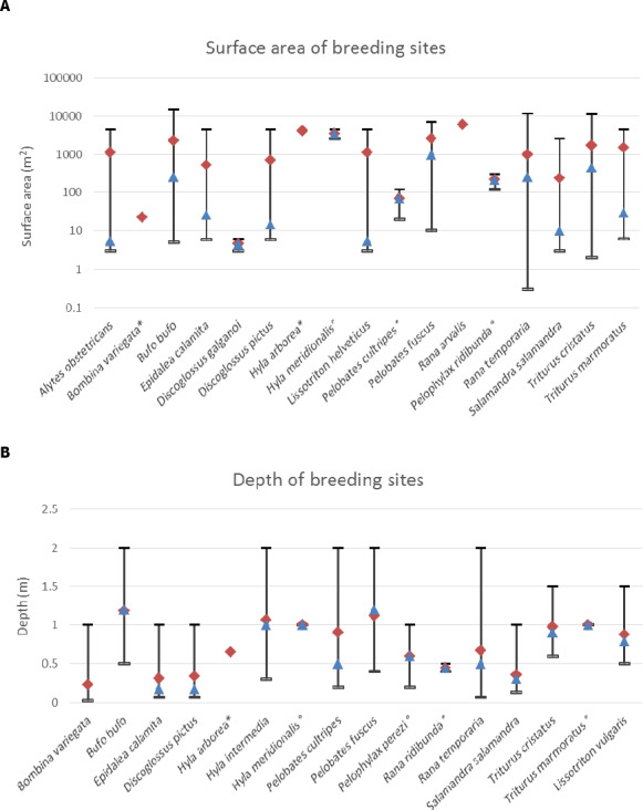
Ranges of surface area (A) and depth measurements (B) of breeding sites reported in literature for different amphibian species. Medians (blue triangle) and means (red diamond) were calculated from literature values for n ≧ 2. Species for which only two data points were available are marked with a °; species for which only a single mean value was reported are marked with a*
Surface ‐area and water‐depth measurements for sites in which the use as breeding sites was not explicitly stated, or only the presence of adults was reported, were not considered in Figure 28 presented below.
For the ponds used for breeding by 17 amphibian species, the mean surface area ranged from 4.6 to 4,160 m2, while the mean water depth ranged from 0.23 to 1.18 m (see Appendix E). So, these data demonstrate that, the water depth of amphibian breeding sites is relatively shallow (means of 0.23–1.18 m, range up to 2 m deep), even for waters with relatively large water surface areas (up to means of 4,160 m2 with range above 10,000 m2).
Paddy fields
Paddy fields, i.e. flooded fields with rice crop, were only briefly discussed in the Working Group, because they were judged not to be a major habitat of amphibians. It is clear that paddy fields receive agricultural inputs such as fertilisers and pesticides, exposure to pesticides is expected to be considerable and that paddy fields require a separate exposure assessment procedure that will differ from other types of water body. For example, overspray with pesticides will be the rule, while drained water, containing pesticides, from other paddy fields may also be a likely entry route.
Ponds vs. puddles
In the context of this Opinion on amphibians and pesticide regulation, the WG considers ponds in locations that may be in the vicinity of agricultural land (edge‐of‐field or somewhat farther, but still part of the habitat that is relevant in landscape modelling) or within agricultural fields. In the latter case, the (temporary) ponds are surrounded by crops and may receive spray‐drift deposition, but they should never receive any overspray, as pesticide regulation assumes Good Agricultural Practices.
Puddles were defined as being temporary water bodies only, that may be located in‐field and may receive overspray. This implies that exposure will be considerably higher in puddles than in ponds, thus result in greater risks for amphibians. It is a risk manager's decision whether or not to include puddles in the risk assessment and to decide on (a) potential mitigation measures and (b) to judge what consequences this may have with respect to the safe use of the pesticide as well as the farmer's behaviour with respect to puddles. For example, an obligation to establish buffer zones around puddles might lead farmers to fill in the puddles.
Sediment
Bed sediment might be an important environmental compartment for amphibians as they may feed on it as well as hibernate in it. Amphibians may become exposed to pesticides via pore water, the organic matter content or a combination of both. The distribution of PPP between pore water and sediment organic matter depends to a great extent on the sorption capacity of the pesticide and is generally a function of depth in the sediment. Over a year, or years, pesticides may accumulate in sediment. This implies that the maximum PEC in the sediment is generally not immediately after application and accompanying spray‐drift deposition on the water column, but later. The exact timing depends on e.g. the sorption capacity of the compound, the degradation rate in the sediment, the degradation rate in the overlying water column (promoting back diffusion from the sediment into the water), the number of applications, or the organic matter content of the upper sediment.
The sediment is characterised by its properties of dry bulk density, porosity and organic matter/organic carbon content. These properties are a function of depth. There are, however, few data on this, especially for water bodies that host amphibians.
Sediment properties were measured in four watercourses in the Netherlands, located immediately adjacent to an arable or horticultural field and distributed across the country (Adriaanse et al., 2015). They were sampled twice, in June/July and in September 2013, carried water all year round and had a minimum water depth of 20 cm. Sediment cores were sampled by pushing transparent PVC tubes into the sediment; these were frozen and then cut with a belt saw into segments of 0–1, 1–2, 3–5 and 5–10 cm. For each location, five cores were sampled in June/July and again in September. Averages and standard deviations were calculated for dry bulk density, porosity and organic matter content for each segment. The properties vary relatively little with depth. The sediment bulk densities are very low compared to soil bulk densities (0.9–1.8 g/mL, excluding peat soils): they range from 0.09 to 0.40 g/mL for the top 0–1 cm and 0.37 to 0.66 g/mL for the lower 5–10 cm sediment. For porosity, the numbers range from 0.71 to 0.93 for the upper cm and 0.75 to 0.84 for the 5–10 cm segment. For the organic matter content, the numbers are 8.9–30.2% for the 0–1 cm segment and 6.5–22.6% for the 5–10 cm segment.
In the USA, bed sediment was sampled from perennial or seasonal ponds containing actively breeding native amphibian populations and located in proximity to agricultural or urban areas where pesticides were being applied (Smalling et al., 2012). Samples were collected in 2009 and 2010, in early spring and summer during the amphibian breeding season in the states of California, Colorado and Oregon (undeveloped, remote areas without direct pesticide applications) and Georgia, Idaho, Louisiana and Maine (where the sampling sites were in close proximity to either agricultural or suburban areas). The bed‐sediment samples were collected from areas of active sediment deposition. A stainless steel scoop was used to collect the top 2 cm of bed material from multiple points within approximately 1 m2 area, which was passed through a 4 mm mesh sieve before analysis. Percent organic carbon ranged from 0.2% to 36.0% for the 42 sites and was below 10% for the large majority of sites. In exposure assessment for pesticide‐risk assessment, 90th percentile worst‐case exposures are often considered. Depending on whether the exposure is mainly via the pore water or via the organic matter content the 90th percentile worst‐case sediment has 1.2% or 12% organic matter, respectively.
Macrophytes, algae, biofilms, zooplankton
Amphibians have a variable diet composition (Section 2.2.7). Newt and salamander larvae mostly feed on zooplankton, while anuran larvae are vegetarian and feed mainly on periphyton, grazing on sediment, plants or biofilms present on the plants (Figure 29). They may thus become exposed to pesticides sorbed or taken up by the plants/biofilms. Filtering phytoplankton or skimming the scum at the water surface are also very common among anuran tadpoles. Aquatic habitats generally contain one or more types of plants, such as macrophytes (rooted or floating), macroalgae (submerged and floating), floating microalgae or biofilms present on macrophytes. Pesticides sorb to plants (e.g. Crum et al., 1999), or may be taken up by shoots or roots of plants (e.g. Burešová et al., 2013). The mass sorbed (and thus concentration) depends on the sorption capacity of the compound and need to be assessed on a case‐by‐case basis as no standard, accepted process description and compound‐specific parameters are available.
Figure 29.
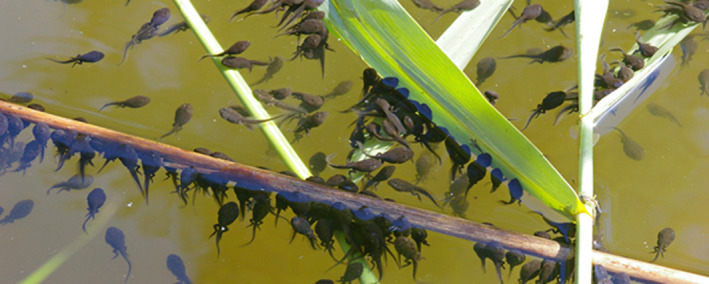
Tadpoles of the common toad (Bufo bufo) feeding by grazing on reed and its biofilms (source: Christian Fisher, CreativeCommons)
9.2.2. Exposure assessment goals and exposure routes for aquatic environment
The elements of the exposure assessment goals linked to the SPG for individual amphibians (no mortality, see Section 6) in their aquatic environment are described in Table 23. The corresponding exposure routes are based upon Table 3 of Section 2.4 and given in Table 24. The EREQs mentioned in Table 24 are proposals. As standard ecotoxicological experiments for amphibians are not yet available for the pesticide‐registration procedure, the final EREQ choice can only be made after a deliberate selection of the most relevant exposure concentration in the potential future ecotoxicological experiment to express the endpoint. (For reasons of simplification the word ‘ponds’ is used in the tables for all temporary or (semi‐)permanent water bodies hosting amphibians).
Table 23.
Elements of the exposure assessment goal for individual juvenile or adult amphibians (SPG: no mortality) in the aquatic environment (in‐field, plus edge‐of‐field)
| Element | Description | Remarks |
|---|---|---|
| EREQ | See Table 24 | |
| Temporal dimension of EREQ | See Table 24 | |
| Spatial unit (SU), type and size (if relevant) | Ponds with surface area of 10 m2 to 2 ha | Implicitly averaging over whole surface area of pond is considered acceptable |
| Statistical population of SUs | All ponds in‐field or edge‐of‐field of treated agricultural fields in area of use of substance | |
| Multiyear temporal statistical population of EREQ values for one spatial unit | Series of tens of years of annual maximum concentration in pond water in years of treatment | Consider only concentrations in periods that are relevant, i.e. when juveniles and adults are present in the ponds |
| Desired spatio‐temporal percentile of the statistical population of EREQ values | Overall 90th percentile of the statistical population of each EREQ | Percentile can easily be changed if needed |
Table 24.
Exposure routes and the definition of the EREQs for individual juvenile or adult amphibians (SPG: no mortality) in the aquatic environment (in‐field, plus edge‐of‐field)
| Exposure route | Source/location | EREQ | Temporal dimension of EREQ | Remarks | |
|---|---|---|---|---|---|
| Contact exposure | Pond water | Spray drift | Concentration dissolved in pond water | Maximum in relevant period of the year | Important route for in‐field ponds, less important for edge‐of‐field ponds located not immediately adjacent to crops |
| Runoff | Important route, also for edge‐of‐field ponds receiving run‐off water from treated fields | ||||
| Drainage | May be important route in case of macropore drainage | ||||
| Atmospheric deposition | Minor route for in‐field ponds. Negligible route for edge‐of‐field ponds (depending on the substance) | ||||
| Oral exposure | Food, plants, water | Daily mass taken in by individual | Maximum in relevant period of the year. | Minor for individuals in ponds, except newts | |
| Inhalation | Air | – | – | Expected to be a minor route compared to oral and contact exposure | |
In chronic risk assessment realistic worst‐case time‐weighted average concentrations may also be used. Annual exposure profiles may be needed e.g. to allow the use of TK‐TD models to predict the effects of the realistic exposure profile.
The size of the spatial unit in the tables below, i.e. the ponds with surface area of 10 m2 to 2 ha, was based upon the following considerations. The minimum pond surface area was set to 10 m2 as the WG judged that (i) smaller ponds usually do not persist sufficiently long to allow larvae to develop into juveniles, (ii) farmers tend to fill in very small ponds, so they do not exist long in the agricultural landscape and (iii) no species could be identified that are specialised in small ponds only. The maximum surface area of 2 ha was mentioned as the upper limit in the pond definition of the UK Countryside Survey (Williams et al., 2010) and was judged to correspond sufficiently with the tendency of amphibians to lay their eggs not too far from the edge of the pond.
Similar tables linked to the SPG for the population persistence (abundance/biomass, distribution and population growth rate, see Section 6) and their corresponding exposure routes have been made (Tables 25 and 26). This covers all life stages of amphibians including eggs, larvae, juveniles and adults. These tables are made consistent with the two standardised amphibian test guidelines available within the OECD framework: AMA (see Section 8.2.2), lasting 21 days and LAGDA (see Section 8.2.1), spanning the period from the embryo stage before hatching (NF 8–10) up to 10 weeks after the median time to reach NF stage 62 in the control group.
Table 26.
Exposure routes and the definition of the EREQs for all life stages of amphibian populations (SPG: population persistence) in the aquatic environment (in‐field, and edge‐of‐field)
| Exposure route | Source/location | EREQ | Temporal dimension of EREQ | Remarks | |
|---|---|---|---|---|---|
| Contact exposure | Pond water | Spray drift | Concentration dissolved in pond water | Maximum or maximum moving TWAa over specified time window for AMA or LAGDA test in the relevant period of the year (length of the time window depends on the endpoint considered, e.g. growth or sex ratio) | Important route for in‐field ponds, less important for edge‐of‐field ponds located not immediately adjacent to crops |
| Runoff | Important route, also for edge‐of‐field ponds receiving runoff water from treated fields | ||||
| Drainage | Possibly an important route | ||||
| Atmospheric deposition | Minor route for in‐field ponds. Negligible route for edge‐of‐field ponds (depending on the substance) | ||||
| Oral exposure | Food, plants, sediment, water | The daily mass taken up by individuals of the population. | Maximum in relevant period of the year |
May be important for a compound with high adsorption capacity such as pyrethroids No spiked food in AMA and LAGDA tests, therefore the main exposure route in AMA and LAGDA tests is via contact (water) |
|
| Breathing | Air | – | – | Expected to be a minor route of exposure compared to contact and oral exposure for juveniles and adults, for aquatic eggs, hatchlings and larvae expected to be unimportant as they do not or hardly breath | |
See the Aquatic Guidance Document (Section 4.5.1 in EFSA, 2013) for criteria when TWA concentrations may be used.
The four tables above focus on the exposure of amphibians in their aquatic environment via water mainly. As mentioned in Table 3 of Section 2.4, however, the underlying sediment may also be an important exposure route, especially for tadpoles feeding on sediment, and for adults that may hibernate in sediment. This is important for compounds that accumulate in sediment, especially when concentrations in the overlying water column are low so that the primary route of exposure is via sediment. There are no standard tests to assess toxicity of pesticides to adults hibernating in sediment, so relating exposure in the field to ecotoxicological effects observed in standard toxicity tests is not possible. From an ecotoxicological point of view, exposure during hibernation is probably mainly via the dermal route as metabolism of the amphibians is low, and, in view of their permeable skin, the ecotoxicological relevant concentration is probably the pore‐water concentration (and not the concentration sorbed to the sediment or the total concentration). The Working Group found two test guidelines for tadpoles from the USA to evaluate risks of pesticides to amphibians, both considering tadpoles exposed by ingestion of and contact with the sediment: (i) the ASTM Whole sediment toxicity tests with amphibians E2591‐07 (2013) and (ii) the EPA Tadpole/sediment subchronic toxicity test OPPTS 850.1800 (1996). The ASTM Guideline uses spiked sediment tests of 10 days with recently hatched tadpoles, sediment concentrations are expressed in mg of active ingredient per kg dry sediment and the overlying water may be renewed by continuous replacement (flow through) or static renewal. The EPA guideline uses spiked sediment of three different natural sediments (organic matter content of 0.1–0.2%, 0.5–1.0% and 2.0–3.0%) and tadpoles before metamorphosis, characterised by the emergence of hind paddles and respiration by gills. The tadpoles are exposed by ingestion, either by direct dosage of spiked slurry into their buccal cavity at the beginning of the test in test chambers with only clean dilution water or by allowing tadpoles to ingest contaminated sediment ad libitum in chambers containing 3–5 cm contaminated sediment and 10–20 cm overlying water. Sediment (and water) concentrations are measured at t = 0 and every 10 days thereafter and sediment concentrations are expressed in mg a.i per kg sediment (dry weight). Based upon the EPA Guideline, which was most explicit in its description with respect to the exposure in the test system, we defined below the elements of the exposure assessment goals linked to the SPG for population persistence (abundance/biomass, distribution and population growth rate) and the corresponding exposure routes in Tables 27 and 28.
Table 27.
Elements of the exposure assessment goal for individual tadpoles (SPG: population persistency) in the sediment of the aquatic environment (in‐field, plus edge‐of‐field)
| Element | Description | Remarks |
|---|---|---|
| EREQ | See Table 28 | |
| Temporal dimension of EREQ | See Table 28 | |
| Spatial unit (SU), type and size (if relevant) | Ponds (with their sediment) with surface area of 10 m2 to 2 ha | Implicitly averaging over whole surface area of sediment in the pond is considered acceptable |
| Statistical population of SUs | All ponds (with their sediment) in‐field or edge‐of‐field of treated agricultural fields in area of use of substance | |
| Multiyear temporal statistical population of EREQ values for one spatial unit | Series of tens of years of annual maximum TWA 30 days concentration in sediment in years of treatment | Consider only concentrations in periods that are relevant, i.e. when tadpoles are present in the ponds |
| Desired spatio‐temporal percentile of the statistical population of EREQ values | Overall 90th percentile of the statistical population of each EREQ | Percentile can easily be changed if needed |
Table 28.
Exposure routes and the definition of the EREQs for individual tadpoles (SPG: population persistency) in the sediment of the aquatic environment (in‐field, plus edge‐of‐field)
| Exposure route | Source/location | EREQ | Temporal dimension of EREQ | Remarks | |
|---|---|---|---|---|---|
| Oral exposure | Main exposure route | ||||
| Sediment | Total concentration in upper x mm layer sediment | Maximum or maximum moving TWAa over specified time window in the relevant period of the year (length of the time window depends on the endpoint considered e.g. growth or sex ratio) | Important route, always present but may depend on feeding mode of tadpole | ||
| Periphyton on water plants | Total concentrations in biofilms on water plants | Importance of route may depend on presence and type of plants and feeding mode of tadpoles | |||
| Other food items (e.g. zooplankton or phytoplankton) | Total concentration in other food items | Importance of route may depend on presence and type of other food items and feeding mode of tadpoles | |||
| Water (i.e. respiration/gill filtration) | Total concentration in water (incl. sorbed on suspended solids) | Important route compared to other oral routes (ingestion) | |||
| Contact exposure | Pond water | Concentration dissolved in pond water | Maximum or maximum moving TWAa over specified time window in the relevant period of the year (length of the time window depends on the endpoint considered, e.g. growth or sex ratio) | Less important route than oral route | |
| Sediment | Concentration in sediment pore water | Less important route than oral route | |||
See the Aquatic Guidance Document (Section 4.5.1 in EFSA, 2013) for criteria when TWA concentrations may be used.
9.2.3. Terrestrial environment
This section focusses on exposure of adult and juvenile amphibians in their terrestrial habitat only, as these are the only terrestrial life stages of amphibians.
9.2.3.1.
Type of terrestrial habitats
As mentioned in Section 2.2.6 in Europe 38 amphibian species (43% of the amphibian diversity) inhabit arable lands. Off‐field sites are a preferred habitat, but occasionally the occupation of arable areas can be dominant. In other cases, the use of arable fields is restricted to particular activities, such as feeding or moving. Home ranges are generally small and, for many amphibian species, they change with season.
Movement patterns
Section 2.2.6 describes the two most typical movement patterns of amphibians: (i) the breeding migration and (ii) the dispersal of juveniles after metamorphosis both movements are characterised by being massive, implying that if exposure to pesticides is possible, probably high proportions of the population may become exposed. During the breeding season, animals tend to concentrate around water bodies whereas they occupy terrestrial environments during the rest of activity, where they search for food. With respect to breeding habitats (i.e. aquatic), amphibians have a site fidelity, migrating year after year to the same breeding site. These migrations may follow the shortest way or can run along more suitable corridors, which affects the chance that the animals may cross arable, cropped fields and risk becoming exposed to pesticides. Distances may be short (few hundreds of meters) or rather long, e.g. 4 km. The second most typical movement is the dispersal of juveniles after metamorphosis. Dispersal movements tend to be orientated non‐randomly towards the most suitable habitat patches. The movements may go over distances of 1.5 km.
Exposure in agricultural areas
Section 2.2.6 mentions that crossing arable fields during breeding migration may happen and may coincide with pesticide application periods. As migration generally occurs during the night, the risk of direct overspray of amphibians is relatively low. When the animals cross shortly after pesticide application, however, dermal exposure by contact with the oversprayed soil surface may be a significant pathway of pesticide exposure of adult or juvenile amphibians. The animals migrate in early spring while the vegetation cover in crop fields is still very low. This favours easy and quick displacement of the animals and the risks of contact to pesticide residues intercepted by the very low vegetation is probably relatively small compared to the exposure via the soil surface. During daytime resting periods, animals tend to look for refuge in densely vegetated areas, which will often be off‐field. Some species, however, dig themselves to shelter; as ploughed, loose fields facilitate this strategy, individuals may stay for entire days inside crop fields during their breeding migrations. In previously treated fields they may thus become exposed to pesticide residues via, e.g. dermal contact or inhalation.
Off‐crop (in‐field and outside fields) the animals may also become exposed via dermal contact with the soil, or residues intercepted by plants. As the deposition rates off‐crop are lower than in‐crop we expect the exposure to be generally lower off‐crop than in‐crop. The deposition rates off‐crop generally depend on many factors, such as crop type and height, spraying equipment, but also wind speed and wind direction related to field orientation (e.g. in the Netherlands the most common wind direction is southwest, and with the main row orientation of fruit trees being north‐south, the spray‐drift deposition is not randomly distributed around the fruit orchards).
Exposure of amphibians in agricultural areas therefore depends on a range of spatial factors (e.g. in‐crop, off‐crop, distance to crops, numbers of crops cultivated and associated application techniques, soil types) and temporal factors (e.g. amphibian life stage, crop development stage), as well as amphibian species with their characteristic habitat and movement traits.
The two exposure routes: direct overspray and indirect exposure by contaminated soil or plants
For terrestrial amphibians, exposure to pesticides through dermal contact is a primary route of exposure in agricultural landscapes. Direct overspray as well as contact with pesticide intercepted on plants followed by uptake through their permeable skin, or uptake from contaminated soils, mainly by their ventral seat patch, are two possible exposure scenarios. Unlike amniotes, amphibian skin is used both for gas and for water exchange. A ventral seat patch, a highly vascularised region of ventral skin, and aquaporins assist with water movement across the skin. Many amphibians actively place their seat patch in direct contact with a moist substrate and this may contribute to increased susceptibility to pesticides and other contaminants. In particular, applications of pre‐emergent pesticides, which are applied to fields early in the growing season with newly germinated plants, can put amphibians in direct contact with relatively high amounts.
9.2.4. Exposure assessment goals and exposure routes for terrestrial environment
The elements of the exposure assessment goals linked to the SPG for individual amphibians (no mortality) in their terrestrial environment (in‐crop) are described in Table 29. The corresponding exposure routes are based upon Table 3 of Section 2.4 and given in Table 30. Tables 31 and 32 present this for the off‐crop, terrestrial life stage. Note that the in‐crop and off‐crop exposure assessment goals and exposure routes have been described in separate tables, because the statistical populations of Spatial Units and exposure routes are different. The EREQs mentioned in Tables 30 and 32 are proposals. As standard ecotoxicological experiments for amphibians are not yet available for the pesticide‐registration procedure, the final EREQ choice can only be made after a deliberate selection of the most relevant exposure concentration in the potential future ecotoxicological experiment to express the endpoint.
Table 29.
Elements of the exposure assessment goal for individual juvenile or adult amphibians (SPG: no mortality) in their terrestrial environment (in‐crop)
| Element | Description | Remarks |
|---|---|---|
| EREQ | See Table 30 | |
| Temporal dimension of EREQ | See Table 30 | |
| Spatial unit (SU), type and size (if relevant) | Individual amphibians | This implies that each individual amphibian has its own in‐crop exposure depending, e.g. on migration day with respect to application day |
| Statistical population of SUs | All individual amphibians in all treated agricultural fields (generally around 1 to 5–10 ha) in area of use of substance | Risk managers may also opt for the alternative of all individuals in all agricultural fields grown with the crop on the pesticide label |
| Multiyear temporal statistical population of EREQ values for one spatial unit | Series of tens of years of annual maxima of EREQ of individual amphibians in years of treatment | |
| Desired spatio‐temporal percentile of the statistical population of EREQ values | Overall 90th percentile of the statistical population of each EREQ | Percentile can easily be changed if needed |
Table 30.
Exposure routes and the definition of the EREQs for individual juvenile or adult amphibians (SPG: negligible effects on mortality) in the terrestrial environment (in‐crop)
| Exposure route | Source/location | EREQ | Temporal dimension of EREQ* | Remarks | |
|---|---|---|---|---|---|
| Dermal exposure | Direct | Overspray | Mass of substance deposited per individual amphibian divided by its body mass | Maximum in relevant period of the year (i.e. when individual amphibians may be present in agricultural fields) | Only important route if migration or other movement occurs during daytime |
| Soil | Residues on soil surface | Concentration dissolved in pore water of upper x cm soil or mass taken up by the individual amphibian | Maximum in relevant period of the year | Important route | |
| Water in puddle on field | Runoff from treated field | Concentration in runoff water or mass taken up by the individual amphibian divided by its body mass) | Maximum in relevant period of the year. | If puddles are formed by runoff in the treated field, this route may be relevant | |
| Plants | Residues on plant leaves | Dislodgeable foliar residue or mass taken up by the individual amphibian (expressed as mass per body mass) | Maximum in relevant period of the year. | May be important especially immediately after spray on low crops (e.g. early growth stages of cereals, all growth stages of salads) | |
| Oral exposure | Food (generally small arthropods) | Daily mass of compound taken in by individual amphibians (mass per body mass) | Maximum in relevant period of the year | See Section 10 for importance of this route | |
| Inhalation | Air | – | – | Inhalation exposure is expected to be a minor route compared to dermal and oral exposure | |
Annual exposure profile may be needed to predict effects by the use of TK‐TD modelling.
Table 31.
Elements of the exposure assessment goal for individual juvenile or adult amphibians (SPG: negligible effects on mortality) in the terrestrial environment (off‐crop)
| Element | Description | Remarks |
|---|---|---|
| EREQ | See Table 32 | |
| Temporal dimension of EREQ | See Table 32 | |
| Spatial unit (SU), type and size (if relevant) | Individual amphibians | |
| Statistical population of SUs | All individual amphibians in all off‐crops strips of land of x m wide in area of use of substance |
Risk managers may also opt for the alternative of all individuals in all off‐crop strips of land adjacent to fields grown with the crop on the pesticide label This implies that each individual amphibian has its own off‐crop exposure, depending on its distance to the treated crop |
| Multiyear temporal statistical population of EREQ values for one spatial unit | Series of tens of years of annual maxima of EREQ of individual amphibians in years of treatment | Consider only EREQs in periods that are relevant, i.e. individual amphibians may be present in off‐crop strips of land |
| Desired spatio‐temporal percentile of the statistical population of EREQ values | Overall 90th percentile of the statistical population of each EREQ | Percentile can easily be changed if needed |
Table 32.
Exposure routes and the definition of the EREQs for individual juvenile or adult amphibians (SPG: no mortality) in the terrestrial environment (off‐crop)
| Exposure route | Source/location | EREQ | Temporal dimension of EREQ | Remarks | |
|---|---|---|---|---|---|
| Dermal exposure | Direct | Spray drift | Mass of substance deposited per individual amphibian divided by body mass | Maximum in relevant period of the year (i.e. when individual amphibians may be present in agricultural fields) | Important route only if migration or other movement occurs in off‐crop strips of land during spray events |
| Atmospheric deposition | Mass of substance deposited per individual amphibian divided by body mass | Maximum in relevant period of the year | Expected to be a minor route and only if migration or other movement occurs in off‐crop strips of land during the periods immediately after spraying | ||
| Soil | Residues on soil surface | Concentration dissolved in pore water of upper x cm soil or mass taken up by the individual amphibian | Maximum in relevant period of the year | Important route | |
| Water in puddle on field | Runoff from treated field | Concentration in runoff water or mass taken up by the individual amphibian | Maximum in relevant period of the year. | If puddles are formed by runoff in the close vicinity of sprayed crops this route may be important | |
| Plants | Residues on plant leaves | Dislodgeable foliar residue or mass taken up by the individual amphibian divided by body mass | Maximum in relevant period of the year. | Expected to be less important as in crop | |
| Oral exposure | Food (generally small arthropods) | Daily mass of compound taken in by individual amphibian | Maximum in relevant period of the year | See Section 10 for importance of this route | |
9.3. Exposure of reptiles
9.3.1. Life stages and habitats
This section focuses on reptile life stages and habitats, based upon Sections 2.3.5 and 2.3.6, and the possible ways of pesticide exposure of reptiles. For most reptiles, all life stages are terrestrial. Reproduction can be broadly divided into two groups: viviparity (approximately 20% of squamates) and oviparity (most common). Viviparity is an adaptation to cold climates and viviparous species generally give birth in early summer. Oviparous species generally lay eggs in late spring or early summer and hatching occurs in late summer. The relevant exposure window may differ between these two groups. Egg nests are located at carefully selected sites, because egg development depends on favourable environmental conditions, such as temperature, water and oxygen availability. Reptilian eggshells are permeable to water diffusion and water is used in the yolk metabolism. This implies that pesticides may enter the egg with the absorbed water and potentially affect the embryonic development. This may occur especially for agroecosystem‐inhabiting populations that sometimes prefer loose soils for nesting, such as freshly ploughed or otherwise cultivated soils.
The majority of continental reptiles are generally sedentary. Their home ranges are better defined than for amphibians and territorialism is not uncommon. Their exposure pattern may therefore be relatively stable: animals inhabiting exposed areas will be almost chronically exposed, while individuals inhabiting non‐exposed areas will have little chances of entering in contact with pesticides. Dermal exposure of juveniles or adults may occur via direct overspray or spray‐drift deposition during pesticide application or contact with contaminated soils, including granules or treated seeds. Dermal exposure by contact with water can happen in puddles inside fields. In addition, some species like terrapins or water snakes are semi‐aquatic and spend long periods of time in water bodies. Thus the exposure routes of runoff, drainage, drift, or atmospheric deposition to water bodies may be relevant for reptiles in a number of cases.
As for amphibians in agricultural areas, exposure for reptiles needs to be assessed in‐crop as well as off‐crop, (in‐field and outside fields). The exposure is dependent on a range of spatial factors (e.g. in‐crop, off‐crop, distance to crops, numbers of crops cultivated and associated application techniques, soil types) and temporal factors (e.g. reptile life stage, crop development stage), as well as reptile species with their characteristic habitat and movement traits.
9.3.2. Exposure assessment goals and exposure routes
The WG limited the exposure assessment goals for the reptiles to the terrestrial habitat, as this is most frequent for reptiles; the WG did not consider semiaquatic species. The elements of the exposure assessment goals linked to the Specific Protection Goal for individual reptiles in‐crop (no mortality) are described in Table 33. The corresponding exposure routes are based upon Section 2.4 for reptiles and given in Tables 34, 35–36 present this for the off‐crop habitat. Similar to what was done for the terrestrial environment of amphibians, we described the in‐crop and off‐crop exposure assessment goals and exposure routes for reptiles in separate tables, because the statistical populations of Spatial Units and exposure routes are different. The EREQs mentioned in Tables 34 and 36 are proposals. As standard ecotoxicological experiments for reptiles are not yet available for the pesticide‐registration procedure, the final EREQ choice can only be made after a deliberate selection of the most relevant exposure concentration in the potential future ecotoxicological experiment to express the endpoint.
Table 33.
Elements of the exposure assessment goal for individual juvenile or adult reptiles in‐crop (SPG: no mortality)
| Element | Description | Remarks |
|---|---|---|
| EREQ | See Table 34 | |
| Temporal dimension of EREQ | See Table 34 | |
| Spatial unit (SU), type and size (if relevant) | Individual reptiles | This implies each individual reptile has its own in‐crop exposure depending e.g. on migration day with respect to application day |
| Statistical population of SUs | All individual reptiles in all treated agricultural fields in area of use of substance | Risk managers may also opt for the alternative of all individuals in all agricultural fields grown with the crop on the pesticide label |
| Multiyear temporal statistical population of EREQ values for one spatial unit | Series of tens of years of EREQ of individual reptiles in years of treatment | As reptiles are quite sedentary, they may be in‐crop during the entire year, so no relevant periods are to be distinguished as is needed for amphibians |
| Desired spatio‐temporal percentile of the statistical population of EREQ values | Overall 90th percentile of the statistical population of each EREQ | Percentile can easily be changed if needed |
Table 34.
Exposure routes and the definition of the EREQs for individual juvenile or adult reptiles in‐crop (SPG: no mortality)
| Exposure route | Source/location | EREQ | Temporal dimension of EREQ | Remarks | |
|---|---|---|---|---|---|
| Dermal exposure | Direct | Overspray | Mass of substance deposited per individual reptile divided by body mass | Annual maximum | Annual maximum may occur after several consecutive applications. Animals may stay in the field the whole year |
| Soil | Residues on soil surface. | Total concentration in specified soil layer | Annual maximum | Possibly important –the ventral skin was more permeable than the dorsal skin | |
| Plants | Residues on plants | Mass deposited on plants | Annual maximum | Possibly important, e.g. when residing in grass | |
| Water in puddle on field | Runoff from treated field | Concentration in runoff watera | Annual maximum | Likely to be minor route of exposure | |
| Oral exposure | Food (including secondary poisoning) | Daily mass of compound taken in by individual reptile | Annual maximum | Important route, see Section 10 (coverage of reptiles by birds and mammals) | |
| Water | Concentration in runoff watera | Annual maximum | Highest concentrations are expected for drinking water from puddles in crop | ||
| Soil | Daily mass of compound taken in by individual reptile | Annual maximum | Probably accidental ingestion of soil (occasionally surpassing the 5% of the diet) | ||
| Inhalation | Air | – | – | Inhalation exposure is expected to be a minor route compared to dermal and oral exposure | |
Table 35.
Elements of the exposure assessment goal for individual juvenile or adult reptiles off‐crop (SPG: no mortality)
| Element | Description | Remarks |
|---|---|---|
| EREQ | See Table 36 | |
| Temporal dimension of EREQ | See Table 36 | |
| Spatial unit (SU), type and size (if relevant) | Individual reptiles | This implies that each individual reptile has its own off‐crop exposure, depending on its distance to the treated crop |
| Statistical population of SUs | All individual reptiles in all off‐crops strips of x m wide and adjacent to treated fields | Risk managers may also opt for the alternative of all individuals in all off‐crop strips of land adjacent to fields grown with the crop on the pesticide label |
| Multiyear temporal statistical population of EREQ values for one spatial unit | Series of tens of years of EREQ of individual reptiles in years of treatment | As reptiles are quite sedentary, they may be in‐crop during the entire year, so no relevant periods are to be distinguished as is needed for amphibians |
| Desired spatio‐temporal percentile of the statistical population of EREQ values | Overall 90th percentile of the statistical population of each EREQ | Percentile can easily be changed if needed |
Table 36.
Exposure routes and the definition of the EREQs for individual juvenile and adult reptiles off‐crop (SPG: no mortality)
| Exposure route | Source/location | EREQ | Temporal dimension of EREQ | Remarks | |
|---|---|---|---|---|---|
| Dermal exposure | Direct | Spray drift | Mass of substance deposited per individual reptile divided by body mass | Annual maximum | Different exposure on the ground or on vertical structures (trees or stone walls) |
| Atmospheric deposition | Mass of substance deposited per individual reptile divided by body mass | Annual maximum | Expected to be a minor route during periods immediately after spraying | ||
| Soil | Residues on soil surface | Total concentration in specified soil layer | Annual maximum | Expected to be minor route, close to crops where spray‐drift deposition onto soil occurred | |
| Plants | Residues on plants | Mass deposited on plants | Annual maximum | Expected to be minor route, close to crops where spray‐drift deposition onto plants occurred | |
| Oral exposure | Food (including secondary poisoning) | Daily mass of compound taken in by individual reptile | Annual maximum | Important route, see Section 10 | |
| Water | Concentration in runoff water | Annual maximum | Highest concentrations are expected for drinking water from puddles formed by runoff water from treated fields | ||
| Soil | Daily mass of compound taken in by individual reptile | Annual maximum | Reptiles are known to ingest soil either by accident when capturing prey, or on purpose for nutrient enrichments | ||
Additional tables linked to the SPG for population persistence (abundance/biomass, distribution and population growth rate) and their corresponding exposure routes are, for reptiles, limited to the eggs for the in‐crop situation. The off‐crop situation for reptile eggs is expected to be of minor importance compared to the in‐crop situation. As no standard accepted methods exist for pesticide registration to evaluate the effects of egg development on abundance/biomass, distribution and population growth of reptiles, the EREQs presented in Tables 37 and 38 are proposals that may need to be adapted later.
Table 37.
Elements of the exposure assessment goal for reptile eggs in nests in‐crop (SPG: population persistence)
| Element | Description | Remarks |
|---|---|---|
| EREQ | See Table 38 | |
| Temporal dimension of EREQ | See Table 38 | |
| Spatial unit (SU), type and size (if relevant) | A nest with eggs | This implies that each nest has its own in‐crop exposure |
| Statistical population of SUs | All nests in all treated agricultural fields in area of use of substance | Risk managers may also opt for the alternative of all nests in all agricultural fields grown with the crop on the pesticide label |
| Multiyear temporal statistical population of EREQ values for one spatial unit | Series of tens of years of EREQ of nests in years of treatment | Consider only EREQs in periods that are relevant, i.e. when nests with eggs are present in the agricultural fields (late spring to late summer) |
| Desired spatio‐temporal percentile of the statistical population of EREQ values | Overall 90th percentile of the statistical population of each EREQ | Percentile can easily be changed if needed |
Table 38.
Exposure routes and the definition of the EREQs for reptile eggs in nests in‐crop (SPG: population persistence)
| Exposure route | Source/location | EREQ | Temporal dimension of EREQ | Remarks | |
|---|---|---|---|---|---|
| Contact exposure | Soil | Residues in soil | Total mass of substance in specified soil layer absorbed by all eggs in nest | Maximum in relevant period in the year | Only (and thus most important) route of contact exposure of eggs |
9.4. Conclusions
The analysis of the dimensions of the Spanish and Swiss amphibian ponds and the CountrySide Survey ponds in the UK (Appendix C) demonstrates that most of them (70–90%) are considerably smaller than the FOCUS ponds, used at present in the aquatic risk assessment at EU level. We therefore expect peak concentrations in FOCUS ponds not to be conservative estimates for those in the analysed ponds. For peak concentrations in FOCUS ditches and streams, the WG was unable to make a general statement on their conservativeness compared to those in the analysed ponds. In view of the higher flow‐through rates in the FOCUS ditches and streams, the pesticide concentrations are expected to decline rapidly and thus they probably represent underestimates of chronic exposure in ponds in the areas surveyed.
The use of Exposure Assessment Goals defines the spatial unit with its EREQs. However, exposure routes allow for an explicit and systematic methodology to calculate PECs in the field, for amphibians in their aquatic and terrestrial environment and for reptiles.
10. Coverage of risk to amphibians and reptiles by existing RA for other groups of organisms (including human RA)
10.1. Introduction
It has been assumed up to now that the risk to amphibians and reptiles is covered by the current risk assessment on surrogate species such as birds, mammals or fish. When analysing this assumption, the question arises as to what exactly is implied by this. The regulation (EC) No 1107/2009 for plant protection products requires that ‘substances should only be included in plant protection products where it has been demonstrated that they present a clear benefit for plant production and they are not expected to have any harmful effect on human or animal health or any unacceptable effects on the environment’. In order to assess the acceptability of the effects, the toxicity of the substance to non‐target organisms needs to be compared with exposure levels that may result from the application of a specific compound in the environment, while considering the uncertainties in the approach, which evolve from the assumptions and extrapolations done for the assessment. Ultimately, the acceptability of the effects is defined by the protection goals.
The uncertainties are addressed by applying assessment factors (AF) in the risk assessment. According to the Technical Guidance Document for Chemicals (European Commission, 2003) the following has to be taken into account when choosing the appropriate assessment factor:
Intra‐ and interlaboratory variation of toxicity data
Intra‐ and interspecies variation of toxicity data
Short‐term to long‐term/chronic toxicity extrapolation
Extrapolation from single species laboratory data to field impact on ecosystems
While there are substantial data that demonstrate the uncertainty for the first three bullet points for fish (European Commission, 2002), there are limited data available for amphibians and reptiles. It is therefore unknown at present whether the same assessment factors as for fish can be applied to amphibians and reptiles.
A comparison of toxicity endpoints from fish with amphibians was done in the aquatic guidance document (EFSA PPR Panel, 2013) where it was concluded that ‘rainbow trout is a good surrogate test species for predicting the acute toxicity of PPPs for larval stages of amphibian species living in the aquatic compartment of the environment. By using the same AFs as have been applied for fish, the achieved level of protection will be the same for both groups of organisms’. It is important, however, to differentiate between the coverage of risk and the coverage or even predictability of toxicity.
Even though the comparison is considered appropriate and valuable, the comparison of toxicity endpoints does not allow a judgement on the achieved level of protection. This is due to the rather limited data set available for amphibians, focusing on one species (X. laevis, 87 of 253 data points with 48 species, 34%). A range of unresolved issues stem from this, such as the representativeness of the tested species as well as the variability in sensitivity between species, populations and life stages.
Furthermore, the statement implies that the exposure of amphibians in the aquatic environment is comparable to fish without providing further details. Therefore, in the following, first an evaluation of the available toxicity studies with surrogate species and then an assessment of the suitability of the available exposure models is provided before addressing the coverage of amphibians and reptiles in the current risk assessment scheme.
In the current risk assessment, a limited number of species and life stages are tested mainly for direct effects via limited and separate routes of exposure, but predictions are made for entire populations living in a landscape. The coverage and conservatism of the current scheme for all substances and non‐target species in the long term is unknown at present.
10.2. Coverage of aquatic life stages of amphibians and reptiles in the current risk assessment for aquatic organisms
This section analyses endpoints and exposure models used in the aquatic risk assessment and makes a comparison with likely exposure and effects in amphibians and reptiles.
10.2.1. Extrapolation of endpoints observed in fish to amphibians and reptiles
Standardised test protocols are available for fish and the endpoints could be available in the dossiers as standard requirements (see Appendix F). According to the data requirement (Commission Regulation (EU) No 283/2013), an acute toxicity testing is always required for rainbow trout (Oncorhynchus mykiss). Chronic studies (early life stage or fish full life cycle) are required depending on the stability of the active substance. A bioconcentration study is required depending on the log Pow and the stability of the active substance. Further studies may be required if the substance is a potential endocrine disruptor. When accumulation of an active substance in aquatic sediment is indicated or predicted by environmental fate studies, the impact on a sediment‐dwelling organism needs to be assessed by determining the chronic risk to Chironomus riparius or Lumbriculus spp.
The observed effects in studies with fish can be summarised into six categories, namely effects on survival, appearance, size, behaviour and reproduction as well as effects on the endocrine system. Endocrine and reproductive toxicity are discussed in Section 8.
Acute endpoints, which are based on mortality, are considered comparable and it is desirable in order to limit animal testing to use the LC50 from fish to cover the acute sensitivity of amphibians and reptiles. However, it needs to be defined what percentage of data points needs to be covered. Is the sensitivity of amphibians and reptiles covered by fish, based on a statistical evaluation of the acute endpoints, if all, the majority or the mean of all endpoints is higher than for fish? The question is whether the toxicity of new substances can be predicted based on the available data.
Sublethal endpoints are more difficult to compare as the exposure time may not be identical. Also the significance of a sublethal effect observed in the laboratory on a population in nature is difficult to predict. Sublethal concentrations of pesticides may affect survival of amphibians by increasing the susceptibility of eggs and larvae to pathogens or diseases (Carey and Bryant, 1995) by altering the immune system (Mann et al., 2009). By retarding growth and metamorphosis, the time the young depart the breeding pond may be affected or the vulnerability to size‐specific predation. Furthermore, the ability of young to avoid predators may be inhibited by sublethal concentrations, i.e. by causing deformities in the body or tail or by reducing swimming performance (Carey and Bryant, 1995).
Missing endpoints, which cannot be covered by fish and might be needed due to the special biology of amphibians, are for instance effects on metamorphosis and certain effects on the reproductive system (see Section 8). The reproductive physiology of amphibians shows a closer relationship with higher vertebrates than with that of fish. For instance, in amphibians and higher vertebrates, testosterone and dihydrotestosterone are the main androgenic sex hormones, whereas in fish it is 11‐ketotestosterone (reviewed in Kloas and Lutz, 2006). Another major difference between fish and amphibians is that the Müllerian ducts, which are the embryonic precursors of the female reproductive tract (uterus, oviducts) in vertebrates, are absent in teleost fish (in which the sex duct has a different ontogenetic origin) (Adkins‐Regan, 1987). It is therefore not possible to extrapolate the effects of chemical exposure from fish to amphibians with regard to impact on the development of the female reproductive system due to fundamental anatomical differences. But that does not exclude the possibility that the sensitivity of the endpoints in sexual development toxicity tests in fish is not comparable to those in amphibian tests, to certain chemical exposures. Ethinyl estradiol exposure affects sexual development in fish and amphibians at comparable exposure levels (about 1 ng/L). the effects however are different; in fish testicular development is affected whereas in amphibians (and reptiles, birds, mammals) both testicular and female oviduct development are affected. Thus, the hazard of chemicals that specifically target female reproductive development may be overlooked using fish tests.
An exposure of aquatic life stages can lead to effects that are carried over into adult amphibians. Whereas decrease in mass at metamorphosis in the aquatic environment after a single exposure to a short‐lived contaminant (carbaryl) was overcome in the terrestrial environment by spring emergence (Boone, 2005; Distel and Boone, 2009, 2010), other studies suggest that sublethal effects on larval growth and development may impair amphibian populations permanently. Embryonic and larval exposure to atrazine altered the behaviour and increased the dehydration rate of post‐metamorphic Ambystoma barbouri eight months after exposure (Rohr and Palmer, 2005). Endocrine effects may lead to skewed sex ratio or sterility in adults (Pettersson et al., 2006; Gyllenhammar et al., 2009; Hayes et al., 2010; Berger et al., 2011; Kvamryd et al., 2011) and thus affect reproduction. Due to the biphasic life‐history amphibians face, a double jeopardy of exposure stemming from terrestrial and aquatic environments (Todd et al., 2011). Thus, long‐term and carry‐over (postexposure) effects spanning several life stages, which may have greater consequences on populations than transient effects, need to be addressed.
As with fish, ontogenic variation in vulnerability to pesticides has been reported, but may be difficult to generalise. Whereas the jelly coat of the eggs may protect embryos from some substances, insufficient protection by the jelly coat has been observed after the exposure of Rana arvalis eggs to cypermethrin (Greulich and Pflugmacher, 2003) leading to abnormalities in the hatched embryos. The sensitivity of larvae may be determined by the development of organs and thus depends on the mode of action of the active substance. The time of metamorphosis may be particulary sensitive due to the physiological demands through that developmental time. Also the ability to detoxify pollutants in different life stages affects the sensitivity as well as the thickness of the skin.
A further, significant difference may be the duration to effects after exposure due to different rates of metabolism. The metabolic rate is influenced by temperature and is thus very variable. Toxicants may be metabolised faster and thus not reach a threshold value, but a faster metabolism could also increase the energetic demand and thus increase uptake of a chemical orally or by inhalation.
10.2.2. Potential coverage in toxicity – comparison of fish toxicity with toxicity values for amphibians and reptiles
A limited number of published comparisons is available for amphibians only and will be summarised in the immediately following text. Further comparative work will be conducted within the framework of the procurement OC/EFSA/PRAS/2015/01 and may be considered at a later point. No comparative data could be found for reptiles.
Acute data
Acute toxicity data of freshwater species developed by the U.S. Fish and Wildlife Services from 1965 to 1986 were analysed with regard to taxonomic differences (Mayer and Ellersieck, 1986). In this data set of 14 insecticides (2 carbamates, 6 organochlorines and 6 organophosphates), amphibians were the least sensitive group compared to insects, crustaceans and fish. Testing three species (Daphnia, Gammarus and rainbow trout) provided the lowest toxicity value 88% of the time. The suggestion was that, by testing a limited set of species, the range of sensitivity of all species could be determined. The working assumption for USEPA is therefore, that toxicity data for fish are broadly protective of aquatic‐phase amphibians and that oral/dietary toxicity data for birds are broadly protective of terrestrial‐phase amphibians.
Hoke and Ankley (2005) concluded, based on a limited data set (atrazine, malathion, parathion), that traditional aquatic test species (primarily cladoceran, fish) are generally more sensitive than FETAX (X. laevis) when comparisons are based on lethality data. They also pointed out, however, that growth is the more sensitive endpoint from FETAX.
Birge et al. (2000) compared the acute toxicity of fish and amphibians for organic compounds (atrazine, phenol, chloroform, carbon tetrachloride, NTA and methylene chloride) and concluded that amphibians were acutely more sensitive than rainbow trout in 35% of the comparisons.
Kerby et al. (2010) noted that a number of authors have investigated the sensitivity of amphibians to pollutants, but no clear indication of the overall sensitivity could be derived. They conducted an extensive review using a species‐sensitivity‐distribution (SSD) approach and analysed the median lethal concentration (LC50 24–96 h) data from almost 24,000 studies with aquatic species retrieved from the AQUIRE database of the USEPA to compare the sensitivity of 44 amphibian species with that of other groups of organisms. They concluded that amphibians (eggs and larvae) are of low to moderate sensitivity to metals, inorganic chemicals, and pesticidal active substances (pyrethroids, carbamates, organophosphates or organochlorines) when compared with 13 other classes of organisms, including fishes. The estimated acute hazard concentration values (HC50 values, as usually derived from SSD) were above the average estimates for all taxa analysed signifying an overall low relative acute sensitivity. They found, however, that amphibians were highly acutely sensitive to three phenolic chemicals and add that the average low sensitivity of amphibians does not mean that highly vulnerable amphibian species are not impacted. As one example, the Tiger Frog (Rana tigrina) is strongly sensitive to the organophosphate endosulfan.
Toxicity values for fish and amphibians have been compared (Aldrich, 2009; EFSA PPR Panel, 2013; Weltje et al., 2013) to determine whether standard tests with fish required for the dossiers for active substance evaluation would be likely to cover the potential risk to amphibians present in the surface water.
In the study by Aldrich (2009), acute endpoints for aquatic invertebrates were also included in the comparison as the first tier, acute aquatic risk assessment is triggered by the lowest endpoint of all aquatic organisms. Here, the data were extended with endpoints for aquatic plants (Figure 30). The data for amphibians were obtained through literature search and taken from the databases PAN Pesticide and ECOTOX and cross‐referenced with the original literature. The data for the surrogate species were taken from the EFSA conclusions on individual active substances. The majority of data was found for herbicides and insecticides and 24 substances from 14 different chemical groups could be compared. In 11 cases aquatic invertebrates reacted most sensitively, in two cases fish, in 10 cases aquatic plants and in one amphibians were most sensitive (dimethoate) (see Figure 30). For dimethoate, the variability in the published endpoints for amphibians was rather large.
Figure 30.
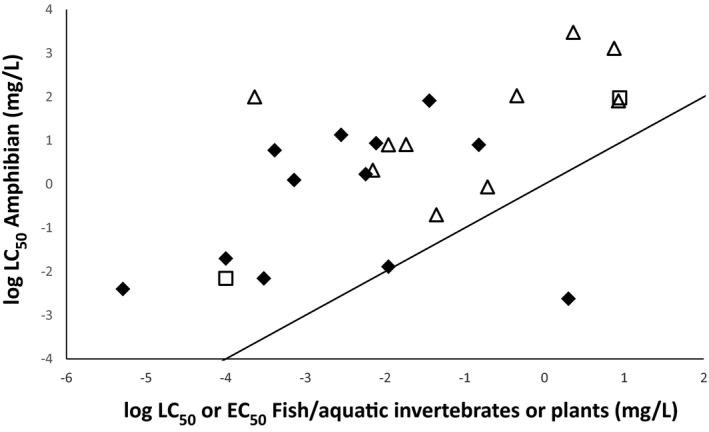
Comparison of the acute sensitivity (log LC 50) of amphibians with the lowest acute endpoint of fish (open square), aquatic invertebrates (filled diamond) or aquatic plants (open triangle) for 24 active substances
A review (Weltje et al., 2013) compared acute and chronic toxicity data obtained from the U.S. Environmental Protection Agency (USEPA) ECOTOX database supplemented with data from the scientific and regulatory literature. Acute data were collected for amphibian species and either rainbow trout (Oncorhynchus mykiss) or fathead minnow (Pimephales promelas) (Figure 31). Only tests from ECOTOX that reported measured concentrations of test chemical were included. A geometric mean value was calculated if more than one 96‐h LC50 value was available for the same chemical and species. When data on several amphibian species were available, only data for the most sensitive amphibian species were selected for further analysis. The comparison was based on 55 chemicals (eight inorganic chemicals and 47 organic chemicals, of which 32 were pesticidally active from 13 different chemical groups). The overall outcome was that fish and amphibian toxicity data were highly correlated using Spearman's correlation (rs = 0.81). Amphibians were more sensitive than fish in 16 of 55 cases (29%). For four of the 55 chemicals, amphibians were between 10‐ and 100‐fold more sensitive than fish and for two chemicals more than 100‐fold more sensitive. After a detailed inspection of these two cases, however, the authors of the study (Weltje et al., 2013) concluded that fish are appropriate representative species to cover the sensitivity of aquatic vertebrates in current risk assessment procedures. Only substances that specifically interfere with biochemical pathways involved in amphibian metamorphosis may not be detected when using fish as surrogates.
Figure 31.
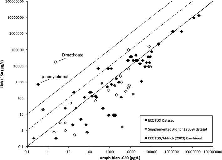
Relationship between amphibian and fish median acute lethal concentration (LC50) values. The solid line delineates the 1:1 relationship. The dashed line delineates a factor of 10. The dotted line delineates a factor of 100, which is the standard EU assessment factor applied to fish acute toxicity data for plant protection products. (Weltje et al., 2013)
A further comparison by Weltje and Wheeler (2015) focused on the comparison of the acute sensitivity of a tropical amphibian species, tadpoles of the red‐eyed tree frog (Agalychnis callidryas), with fish. The LC50 data for the tadpoles were determined after 8‐day exposure in a semistatic test based on nominal concentrations using commercial formulations (Ghose et al., 2014). The 96 h LC50 values for fish were collected from the Pesticide Properties DataBase or USEPA REDs. The comparison for the ten active substances indicated higher sensitivity of fish for eight substances. The apparently higher sensitivity for glyphosate and paraquat of A. callidryas was possibly attributed to the longer exposure time, increased toxicity due to the formulation or unconfirmed test concentrations. The study authors conclude that fish are suitable surrogates to cover the sensitivity of aquatic stages of a tropical amphibian species and that the standard assessment factors cover the extrapolation to potentially more sensitive species and other uncertainties.
The comparison in the aquatic guidance document (EFSA PPR Panel, 2013) used the data collected by Fryday and Thompson (2012) on amphibian species exposed in water. In total, 253 data points for 48 amphibian species including several life stages (e.g. tadpoles/larvae and embryos) with corresponding rainbow trout values were available, from tests with an exposure duration of 96 h on 60 different pesticidal active substances performed under either a flow‐through or a static‐renewal system. Most of the tested species belonged to the subclass of Anura (frogs and toads) and seven of the tested species to the subclass Caudata (salamanders or newts). No data for adults were included in the analysis.
The comparison of the data revealed that in 62% of the cases the rainbow trout is more sensitive than the amphibian species (points above the 1:1 line on Figure 32) and thus in 38% of the cases amphibian species are more sensitive than rainbow trout. If the assessment factor of 100 used for the acute risk assessment of fish is applied to cover the variability between species, then in 2% of the cases the amphibian test species is more than a factor of 100 more sensitive than the rainbow trout (values below the red line in Figure 32). In those cases, the LC50 for amphibians would be lower than the RAC based on the rainbow trout. Repeating this analysis but splitting it by life stage (i.e. keeping embryos and larvae separate) gave a comparable result to the assessment on the whole data set. Therefore, the results were considered to be valid for both embryos and larvae.
Figure 32.
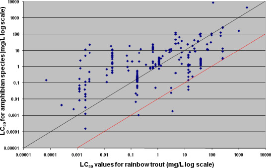
Comparison of each amphibian acute toxicity value with the respective acute toxicity value for rainbow trout (Oncorhynchus mykiss). The black line is the 1:1 line, i.e. the line indicating that the outcome for rainbow trout and amphibians would be exactly the same. The red line considers the assessment factor of 100 applied in the acute risk assessment for fish, i.e. where toxicity to an amphibian would be exactly 100 times higher than toxicity to the rainbow trout (EFSA PPR Panel, 2013)
Based on the same LC50 data for amphibians collected by Fryday and Thompson (2012) and using the acute LC50 for fish listed in the Pesticide Properties DataBase (PPDB database) supplemented by LC50 for thirteen older active substances listed in the aquatic guidance document (EFSA, 2013), the correlation is further investigated here. Only the lowest acute endpoint for amphibians is compared for each of the 85 pesticidally active substances. Unbounded endpoints (>) were included in the comparison. The statistical correlation was investigated with Spearman and Pearson correlation. Although the Spearman correlation assesses the relationship between two variables using a monotonic function, the Pearson correlation assesses linear relationships. For the Spearman's correlation rs = 0.66 (p < 0.0001), whereas for the Pearson correlation r2 = 0.48 (95% confidence interval 0.30–0.63, p < 0.0001) and y = 0.6385x + 0.2732, indicating a weak correlation. The linear regression line has a slope < 1 indicating that for substances where fish react very sensitive amphibians react less sensitive than fish and at concentrations > 1 mg/L (where the linear regression line crosses the 1:1 line) amphibians may react more sensitive than fish (see Figure 33) as the linear regression line is below the 1:1 line.
Figure 33.
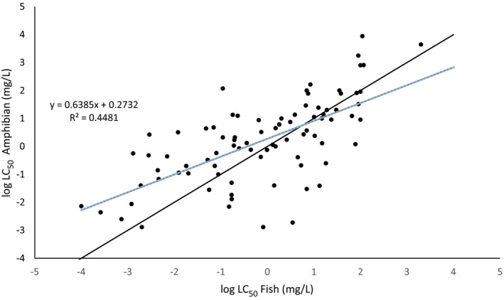
Comparison of the lowest amphibian acute toxicity value with the respective lowest acute toxicity value for fish for 85 active substances. The blue line is the linear regression (r2 = 0.448; y = 0.6385x + 0.2732) and the black line is the 1:1 line, i.e. the line indicating that the outcome for rainbow trout and amphibians would be exactly the same
The uncertainty in the linear regression is presented in Figure 34 with the confidence interval and prediction interval. The width of the prediction interval indicates that a factor of at least 100 may be a suitable extrapolation factor based on the currently available data to predict the LC50 for amphibians from the LC50 for fish.
Figure 34.
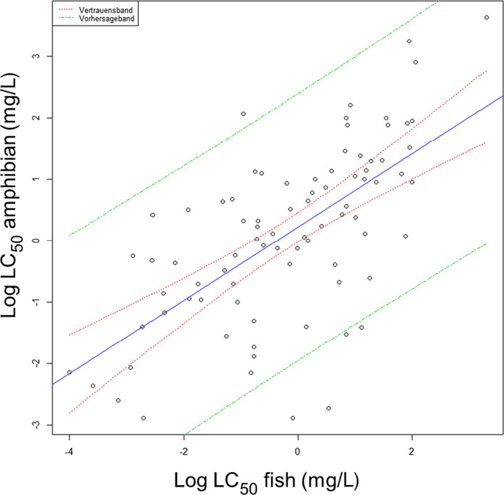
Comparison of the lowest amphibian acute toxicity value with the respective lowest acute toxicity value for fish for 85 active substances. The blue line is the linear regression (r2 = 0.448; y = 0.6385x + 0.2732), the red lines are the confidence interval of the mean and the green lines indicate the width of prediction. For a new substance with a measured LC 50 for fish the LC50 for amphibians can be predicted to lie within the green lines. As the green lines are straight and not curved the prognosis is good. The distance between the blue and the green line indicates that a factor of at least 100 may be a suitable extrapolation factor based on the available data
In the current procedure, the aquatic risk assessment is triggered by the aquatic species showing the greatest risk, which may be based on fish, aquatic invertebrates or aquatic plants (macrophytes and algae). Hence, the data from Fryday and Thompson (2012) were extended with endpoints obtained from the Pesticide Properties DataBase (PPDB database) for aquatic invertebrates and aquatic plants; thus 72 substances could be compared. In nine cases (14%), the lowest endpoint for amphibians was lower than the lowest endpoint of the current surrogate species. When plotted against the currently used RACs (by including the current assessment factors (AF) of 100 for fish and aquatic invertebrates and 10 for aquatic plants), the data indicate that all acute toxicity endpoints (LC50) for amphibians are above those RACs (Figure 35). However, in the context of risk assessment, AF to calculate RACs need to consider all relevant uncertainties. Besides covering the species variability in toxicity, also uncertainties with regard to i.e. exposure need to be considered (see Section 7.11).
Figure 35.
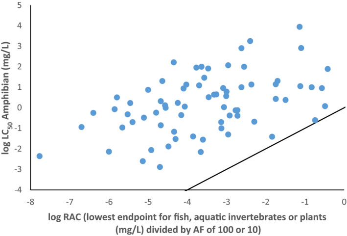
Comparison of the lowest RAC (regulatory acceptable concentration, i.e. lowest endpoint for fish, aquatic invertebrates or plants divided by the current assessment factors of 100 resp. 10) with the respective amphibian acute endpoint. The black line is the 1:1 line, i.e. the line indicating that the outcome for the surrogate species (with assessment factor) and amphibians (without assessment factor) would be exactly the same
Thus, for performing an acute amphibian risk assessment, some elements need to be further addressed, i.e.:
the value of a suitable assessment factor with regard to the relevant uncertainties of the risk assessment and
the value of the extrapolation factor to be applied to the LC50 for fish to cover the acute toxicity for amphibians considering the limited data available with regard to species and life stages tested.
The most frequently tested species in the literature is the African Clawed Frog (X. laevis), whose sensitivity in comparison to European species is not clear. Although Birge et al. (2000), Hoke and Ankley (2005) and Kerby et al. (2010) do not consider X. laevis to be particularly sensitive to any type of chemical, Wagner et al. (2013) describe X. laevis as a sensitive species. Therefore, the sensitivity of European or local species might give a more reliable – and different – estimate of the impacts of PPP on amphibian species. Furthermore, comparing dose–response functions rather than just endpoints would give more information about the respective sensitivities.
Sufficient LC50 values for a number of amphibian species could be found for four active substances to construct species sensitivity distributions (Ortiz‐Santaliestra et al., 2017). The large range in acute sensitivity between amphibian species and the position of Xenopus laevis is apparent (Figure 36), with the endpoint of X. laevis covering in average only about 50% of the other species. Therefore, X. laevis does not seem to be among the most sensitive species. A sensitivity distribution between different amphibian species spanning several orders of magnitude was also noted by Ghose et al. (2014).
Figure 36.
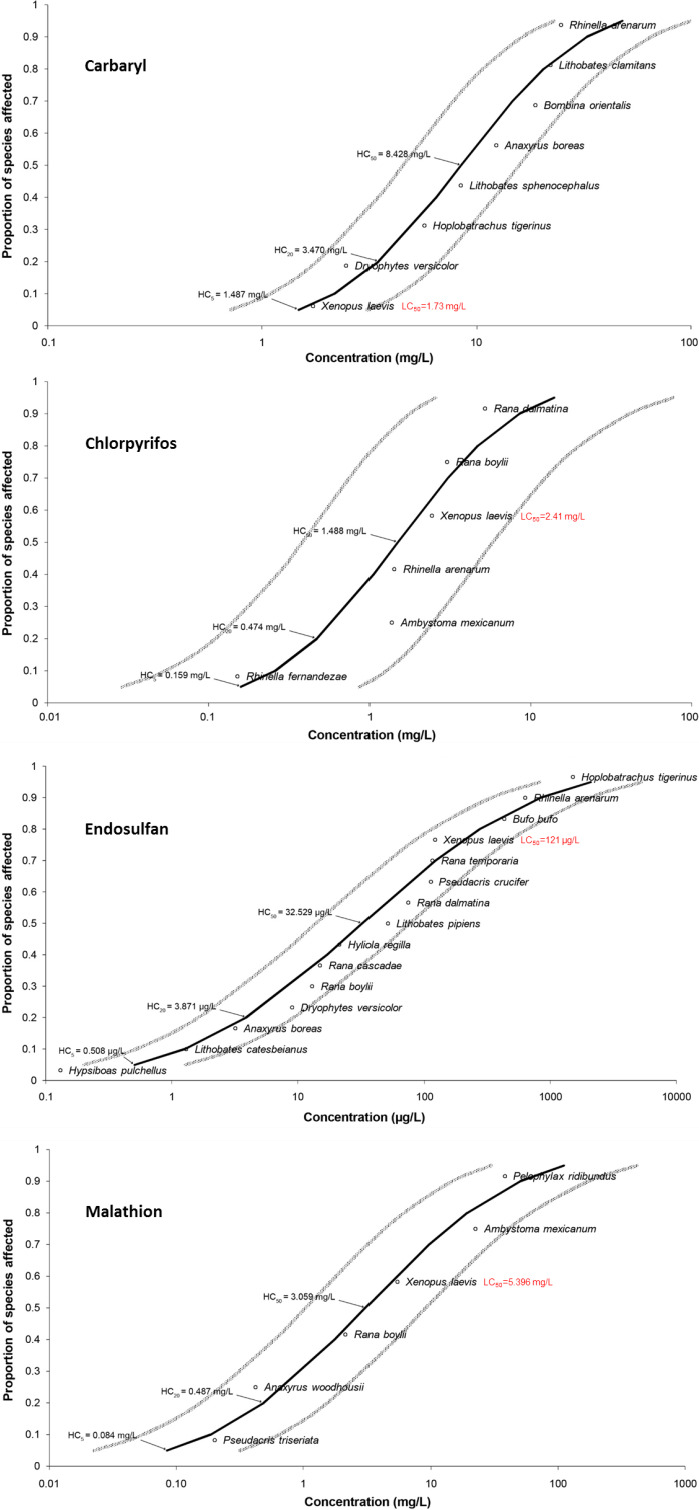
SSD for chlorpyrifos, carbaryl, endosulfan and malathion based on acute LC 50 for 6–15 amphibian species. The sensitivity of Xenopus laevis is marked in red
Chronic data
Birge et al. (2000) listed LC10 values for 12 organic compounds and for 6 substances (phenol, carbon tetrachloride, NTA, methylene chloride, benzene and m‐xylene) the LC10 for amphibians was lower than for fish.
Chronic toxicity data for fish were available for 52 chemicals (10 inorganic chemicals and 42 organic chemicals, of which 20 were pesticidally active substances) (Weltje et al., 2013). Chronic toxicity data were taken from USEPA databases and scientific literature, for fish also from EU or US regulatory dossiers. Data were retained for analysis if they were from studies of at least a 10‐day duration for amphibians and 21‐day duration for fish, employed either static renewal or flow‐through aqueous exposure‐study designs, and reported apical endpoints of potential population relevance (i.e. they were related to survival, growth, development (including metamorphosis), or reproduction). Most of the fish NOEC values are based on measured exposure concentrations, whereas most of the amphibian data are based on nominal concentrations. The amphibian data comprised studies involving 14 amphibian species (predominantly studies using species from the genera Rana, Bufo, and Xenopus). If the NOEC was unbound (i.e. where the highest tested concentration is reported as the NOEC) or the spacing factor was ≥ 100 the studies were considered to be potentially unreliable by the authors, because in these cases, the true NOEC may be higher than the reported value. The study authors conclude that amphibians were more sensitive than fish in 11 of 52 cases (21%) (Figure 37). Amphibians were between 10‐ and 100‐fold more sensitive than fish for five substances and greater than 100‐fold more sensitive for one chemical (sodium perchlorate). The study authors concluded that additional amphibian testing is not necessary during chemical risk assessment (acute and chronic). The PPR panel would like to point out that although chronic endpoints derived from different effects (survival against sublethal effects), different exposure times or specifications of concentration (for fish mainly measured and for amphibians mainly nominal concentrations) were compared. The exposure time for the fish studies was potentially longer (21–396 days, median 37.5 days) compared to the amphibian studies (10–210 days, median 42 days). The Panel therefore does not consider that the study provides sufficient evidence that the chronic risk for amphibians can be assessed based on the NOEC for fish.
Figure 37.
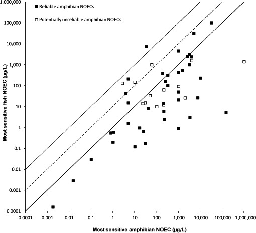
Relationship between chronic amphibian and fish no observed effect concentrations (NOECs). The solid line delineates the 1:1 relationship. The dashed line delineates a factor of 10, which is the standard EU assessment factor applied to fish chronic toxicity data for plant protection products. The dotted line delineates a factor of 100 (Weltje et al., 2013)
The USEPA used ecotoxicity data for a standard amphibian test species (X. laevis), which they received as part of the Endocrine Disruptor Screening Program, for a comparative analysis of chronic effects (Aubee and Glaberman, unpublished data). Although these studies are primarily designed to inform a determination of potential thyroid interaction within the context of other endocrine screening studies, they also contain valuable data on survival and growth, which can be compared with existing fish data for a given chemical. Endpoints were extracted for survival, body weight, and length from EPA reviews (preliminary or final) of industry data submissions for 43 different pesticidal active substances. The analysis considered only pesticidal active substances toxicity and not PPP toxicity. The data set included studies with O. mykiss, P. promelas, and X. laevis. Each laboratory study included at least 21 days of chemical exposure and was conducted according to a standard EPA test design. Data generated according to AMA with juveniles and fish short‐term reproduction assay (FSTRA) with adults were considered. All comparisons were done based on the no observed adverse effect concentration (NOAEC) for a given effect and all endpoints were based on measured test concentrations (mean measured or time‐weighted average). The lowest test concentration was divided by two in cases where the endpoint was non‐definitive (<) because effects were seen at all treatment levels. Unbounded NOECs were not adjusted, but included in the analysis.
In a preliminary analysis of the 43 pesticidally active substances tested in both an amphibian metamorphosis assay and a short‐term fish reproduction assay, statistically significant effects on mortality were seen in amphibians (Xenopus laevis) at lower test concentrations than in fish (Pimephales promelas) 42% of the time (Table 39). Growth parameters in amphibians were affected at lower test concentrations than in fish in 53% (body weight, n = 43) and 59% (length, n = 39) of studies, respectively. (Length was not reported in all fish studies.) The fish NOAEC underestimated the amphibian NOAEC by a factor of at least ten in 8% of cases for mortality, 13% of cases for body weight, and 29% of cases for length. In cases where the amphibian endpoint was lower, particularly for length, the average difference between the amphibian and fish endpoint appeared to be considerably greater than the difference when the amphibian was not more sensitive. Therefore it seems worthwhile to investigate cases where amphibians are more sensitive than fish. On the whole, however, there were no statistically significant differences in NOAEC values for mortality, body weight, and length in amphibians as compared to fish.
Table 39.
Summary statistics for the one‐tailed hypothesis: Are amphibians more sensitive than fish?
| Apical effect (n) | Amphibian NOAEC < fish NOAEC | Amphibian NOAEC > fish NOAEC | p‐value | ||||
|---|---|---|---|---|---|---|---|
| % of cases | Mean diff. | Max diff. | % of cases | Mean diff. | Max. diff. | ||
| Mortality (n = 43) | 42% | −44% | −98% | 58% | 45% | 10E3% | 0.94 |
| Body weight (n = 43) | 53% | −62% | −97% | 47% | 17% | 12E3% | 0.90 |
| Length (n = 39) | 59% | −70% | −99% | 41% | 13% | 11E3% | 0.09 |
The results of this exploratory analysis indicate that, overall, chronic fish ecotoxicity data for exposure to pesticidal active substances provide a reasonable approximation of central tendency for ecotoxicity in amphibians, using model test species. There were no statistically significant differences between NOAEC values for fish and amphibians with respect to mortality, body weight, or length. In cases where amphibians were less sensitive than fish, they were at times far less sensitive – with orders of magnitude in the difference between species. Aubee and Glaberman conclude that, if the purpose of a surrogate is to provide an average representation of effects levels across taxa, then these results indicate that the use of fish to represent aquatic amphibians under chronic exposure conditions remains appropriate.
It is noteworthy, however, that a lower endpoint was derived for amphibians in 42–59% of comparisons. While not statistically significant, this suggests that amphibians may be more sensitive to certain exposures on an individual chemical basis, and, according to the authors, it challenges the traditional notion in ecological risk assessment that fish are consistently more sensitive. Such differences may have an impact in individual chemical risk conclusions, depending on the magnitude of the difference and the environmentally relevant exposure levels as a chronic risk assessment based on fish may not cover the toxicity for amphibians. Finally, the study authors point out the uncertainty in the analysis due to the difference in life stages exposed. Data sets which support cross‐species and life stage‐matched ecotoxicity comparisons are needed.
Conclusion of the comparative studies with fish
Based on the limited data and studies available, the comparison of the acute and chronic sensitivity of amphibians with the standard fish test species, suggests that the sensitivity of amphibians may be covered by fish in some, although not all, cases. Around 30% of the acute endpoints for amphibians are lower than for fish and for the chronic endpoints around 50%. This was confirmed in a review recently conducted for EFSA (Ortiz‐Santaliestra et al., 2017), where it was furthermore concluded that the sensitivity due to other routes of exposure (oral uptake through food or sediment) cannot be compared due to lack of data. In order to cover the acute toxicity to amphibians, an extrapolation factor is suggested for the acute fish endpoint. This extrapolation factor may be derived from the width of the prediction interval from a comparison in sensitivity between fish and amphibian (see Figure 32). Another possibility to conclude on an extrapolation factor is to relate the LC50 from fish to the HC5 derived from species sensitivity distributions (SSD) of LC50 for several amphibian species. However, this requires that sufficient data for a range of active substances is available in order to construct SSDs. Furthermore, how the extrapolation factor would need to be calculated with the other uncertainties that need to be addressed in the risk assessment for amphibians needs to be defined. The limitation of the current analysis is that a comparable endpoint does not indicate a comparable sensitivity when the slope of the dose–response curve is considered. A steep dose–response curve introduces a greater uncertainty in the risk assessment than a flat dose–response curve. The preliminary conclusion is based on a limited data set for less than one hundred pesticidal active substances, especially for the chronic exposure and with regard to the life stages tested. Possibly not the most sensitive chronic endpoint of the most sensitive life stage was used for the comparison due to lack of data questioning the general validity of the comparison. A systematic review indicated that primarily hatchlings, but and also larvae appear to be the most sensitive aquatic life stages depending on the analysed effect (Ortiz‐Santaliestra et al., 2017), whereby most data is available on larvae and data on hatchlings is sparse. The majority of endpoints are available for X. laevis and thus limited conclusions can be drawn about variability in sensitivity between species. Although the rainbow trout (O. mykiss) is generally regarded as one of the most sensitive fish species (even though the location of the rainbow trout within fish species sensitivity distributions should be reaffirmed, see Ortiz‐Santaliestra et al., 2017), the most sensitive amphibian species is currently not known. One question is whether individual cases where amphibians are more sensitive than fish are a reason of concern. Another question is whether the sensitivity of amphibians can satisfactorily be predicted by using fish data and possibly an extrapolation factor. By comparing one endpoint for single species, the distribution in sensitivity for all species cannot be adequately predicted and the whole range may not be covered. Furthermore, the sensitivity may be different in laboratory and mesocosm studies due to other environmental stressors. Based on a limited data set of three pesticides in a systematic review stronger effects were observed in mesocosm studies than in laboratory studies when the same species was compared (Ortiz‐Santaliestra et al., 2017), potentially questioning the usefulness of using laboratory studies with fish to predict direct and indirect effects on amphibians in a pond.
Major gaps in knowledge with regard to toxicity are:
Variability in sensitivity of amphibian species (especially caudates)
Representativeness of the tested species for indigenous species
Sensitivity of different life stages not easily maintained in the laboratory
Lack of comparable chronic toxicity data
Comparability of chronic endpoints of fish and amphibians with regard to their significance for the population level
Significance of low endpoints for amphibians for the selective sensitivity towards specific mode of actions
Other routes of exposure such as food and sediment ingestion.
10.2.3. Potential coverage of the exposure assessment – analysis of available exposure models for aquatic organisms and suitability for amphibians and reptiles
The exposure of aquatic vertebrates to pesticides may be via the water column, organic substrates (i.e. algae, leaf litter) and inorganic substrate (i.e. sediments).
Simulation of the exposure in laboratory studies with surrogate species
In acute laboratory toxicity studies, fish are exposed via water, while no feed is provided (OECD 203). Therefore fish are taking up the test substance dissolved in water via their skin or gills, but not orally via feed. In long‐term toxicity studies, fish are fed daily ([Link], [Link]) or ad libitum (OECD 210). However, as the feed is freshly added and not treated, it does not represent a worst‐case oral exposure. This is of minor relevance for the exposure of fish via the oral or dietary route, as the primary route of uptake of pesticides is via gills (Rankin et al., 1982). In fish, gills are critical organs for respiratory, osmoregulatory and excretory functions.
Oral and dermal exposure via sediment is routinely tested with aquatic invertebrates (i.e. Chironomus sp. [Link], [Link] or Lumbriculus sp., OECD 225) and not fish, even though higher tier studies with fish, especially for highly adsorbing substances, may be conducted in the presence of sediment. Test guidelines for amphibians have been developed, see Section 8. Tadpole oral and dermal exposure via sediment is studied in the ASTM Whole sediment toxicity tests with amphibians E2591‐07 (2013) and the EPA Tadpole/sediment subchronic toxicity test OPPTS 850.1800 (1996).
Routes of exposure of amphibians and reptiles
The exposure of amphibians to PPP differs from fish and varies throughout their life cycle. Although eggs are laid in the central part of the water column (attached to submerged plants) and hence are mainly exposed via water, later terrestrial stages are also exposed via oral uptake of food, contact with soil or plants, air or direct overspray. Even though directly immersed in water, eggs are expected to have a limited uptake of contaminants from the water column due to their gelatinous coating. There is some evidence, however, showing that the gelatinous coating may not protect against all pesticides as it was demonstrated that isoproturon and cypermethrin could enter the eggs despite this coating and have some detrimental effects on tadpole development (Greulich and Pflugmacher, 2002, 2004). The uptake of chemicals can begin shortly after egg deposition, as water moves into the egg capsule (Birge et al., 2000); in the jelly mass, 0.7% of total radioactivity was detected, while 2% was measured in the egg. The thickness of the gelatinous coating may change over time. In very shallow ponds, eggs may be in contact with the sediment. Eggs may also be contaminated via maternal transfer. Little is known about this route of exposure at present, however. Some earlier work indicates that lipophilic compounds may concentrate in eggs via maternal transfer, reducing the concentrations in female frogs, and reach higher concentrations in eggs than in mothers. This is especially true for POPs including organochlorine pesticides (Kadokami et al., 2004; Wu et al., 2012). Data for currently used pesticides is needed. Eggs of reptiles may also be exposed via soil contact. There is evidence showing that eggs laid in agricultural areas with local OC pesticide use will have a higher burden of these contaminants, compared with eggs laid in non‐exposed areas (Stocker et al., 2011). Experimental evidence of soil transfer has been published in snapping turtle eggs (Chelydra serpentina) exposed via the soil to atrazine, simazine, metolachlor, azinphos, dimethoate, chlorpyrifos, carbaryl, endosulfan, captan and chlorothalonil. Except for chlorothalonil, all other pesticides were detected above quantification limit in the eggs. The main drivers for egg transfer appeared to be duration of exposure, the soil concentration, a low sorption to organic carbon and lipid, and a high water solubility. The exact mechanisms of transfer are still unknown, although it is speculated that the primary route of exposure could be the vapour and not the dissolved phase in soil (De Solla and Martin, 2011). After hatching of the eggs, the hatchlings start feeding and can thus additionally be exposed via sediment and feed. As the hatchlings grow and become larvae, internal gills are formed, they start breathing and exposure via air becomes a possible (even though expectedly low) route of exposure. During metamorphosis, feeding stops, lungs are developing, but the main routes of exposure are via sediment and water (see also Section 2.4).
The dermal exposure of reptiles via water is much lower than compared with fish or amphibians, apart from some water‐dwelling snakes and terrapins. Some aquatic turtles rely on water held in their buccal cavity for oxygen uptake and this may also provide a pathway for entry of dissolved chemicals (Linder et al., 2010). The oral uptake of water from drinking or feeding is considered relevant.
Therefore the routes of uptake are
dermal via water, sediment, soil, plants or air,
oral via feed or water and
inhalation.
In the aquatic system, the relevant routes of exposures are considered to be:
dermal exposure to water for amphibians (eggs, hatchlings, larvae, metamorphics, juveniles, adults) and reptiles (water dwelling snakes and terrapins),
dermal exposure to sediment for amphibians (hatchlings, larvae, metamorphosis, and juveniles and adults hiding or over‐wintering on the sediment)
oral exposure via sediment for amphibians (larvae)
oral exposure via feed in the water column for amphibians (hatchlings, larvae) and
oral exposure via water while feeding of amphibians (hatchlings) and reptiles (juveniles, adults).
The current risk assessment is intended to cover the use of a single PPP in a limited time frame. This is especially problematic for amphibians, which may be exposed in the water and transfer the body burden to the terrestrial environment. Also, the terrestrial exposure of adults may vice versa lead to maternal transfer to eggs (Pagano et al., 1999; Kadokami et al., 2004).
A hypothesis is that X. laevis may show greater effects than in fish if exposed via diet for lipophilic compounds, as the dietary uptake is more important for amphibians than for fish. The relevant exposure therefore needs to be determined in laboratory studies in order to achieve an optimal and realistic uptake.
For lipophilic compounds, a possible exposure during metamorphosis is the release of substances accumulated and stored in body tissue during tail resorption (Bernabo et al., 2016).
Suitability of the laboratory studies with aquatic surrogate species to simulate the exposure of amphibians and reptiles in the water system
The dermal exposure in water is likely to be adequately reflected by laboratory studies with fish (OECD 203). Dermal and oral exposure to sediment are simulated in the study design with invertebrates (i.e. Chironimus sp., OECD 218, 219 and Lumbriculus variegatus, OECD 225) only. The oral exposure to pesticides via the dietary route is only partially covered in the long‐term studies with fish. The oral exposure via water is considered to be covered in the acute and long‐term studies with fish as freshwater and marine fish pass water through their stomachs and excrete urine.
Hence, the current aquatic studies with surrogate vertebrates do not adequately cover the dietary route of exposure and dermal exposure via contact to sediment for amphibians and reptiles, whereas the dermal exposure in the water column is adequately reflected. The oral uptake of sediment is expected to be covered by longterm studies with Lumbriculus variegatus, but the comparability of the sensitivity is currently unknown. The relative importance of the dietary route should be determined. Table 40 below provides an overview on life stages and exposure routes and available models to estimate the exposure.
Table 40.
Possible exposure concentrations for amphibians in temporary and permanent ponds (edge of field and in field) for the entry pathways drift, run‐off and drainage
| Life stage | Medium | Available modela | Unit | Description of ecotoxicological exposure quantity |
|---|---|---|---|---|
| Eggs, hatchlings, larvae, metamorphs, juveniles, adults | Water | FOCUS‐sw models | mg/L | Mass of ai dissolved per volume water at average depth (mixed water column) |
| Eggs, hatchlings, larvae, metamorphs, juveniles, adults | Sediment | FOCUS‐sw models | mg/kg | Total concentration in top layer of sediment |
| Eggs | Submerged plant | TOXSWA | mg/kg dry weight macrophyte | Eggs adhered to plants may adsorb the concentration per mass of water plants modelled by TOXSWA |
| Eggs | Maternal transfer | Metabolism studies | mg/kg in egg | |
| Hatchlings, larvae | Food | – (TK/TD) | mg/kg food | Concentration in periphyton, planktonic algae and invertebrates |
Which needs to be adjusted to adequately predict the exposure for amphibians with regard to size of pond, distance to crop, movement of water, field to pond ratio, organic carbon content in the sediment, bulk density and texture of sediment, adsorption coefficient for water plants.
In order to determine the uptake of sediment or food by larvae, the ingestion rate needs to be known.
Shallow ponds (< 1 m) are considered to be quite homogenous as the temperature difference will lead to a daily mixing of the entire water column. So, consecutive daily inputs via drift and run‐off will be rapidly and homogenously distributed in the ponds. Although the amount of suspended matter may be relatively high in these ponds, adsorption and resuspension of pesticides are insignificant for the size of the PEC in the water layer except for compounds with high sorption capacities, such as pyrethroids.
In order to predict the concentration in the aquatic system, not only hydrological parameters, but also the physical‐chemical properties of the substance are taken into account such as degradation (DegT50) and adsorption (Koc). Depending on the route of entry, the adsorption to the sediment may take days or be instantaneous. Temporary water bodies differ from permanent water bodies in many ways (Lahr, 1997) with fluctuating physical (temperature, light, water level) and chemical (oxygen, pH, ionic strength) characteristics. These characteristics may affect the concentration and bioavailability of the PPP in the water system.
Adequacy to predict the concentration in surface waters used by amphibians by the FOCUS models (comparison of scenarios and parameters)
In the aquatic risk assessment at EU level, the FOCUS surface water scenarios are used to evaluate whether safe uses of the a.i. can be identified or whether critical areas of concern exist. Assessing the exposure for amphibians in all fifteen FOCUS water bodies would be in line with the current aquatic risk assessment at EU level. In the current EU registration procedure assessing exposure in ponds only would be considered as being half a scenario, because in the same scenario a stream is situated as well (D4, D5, R1). A safe scenario needs to have low risk for all water bodies defined for that scenario. So, if, e.g. in both the pond and the stream of the R1 scenario the PEC values are lower than the calculated RAC, there would be low risk for the aquatic ecosystem in both water bodies and the R1 scenario would be classified as having low risk. However, if the PEC in the pond is lower than the RAC, while the PEC in the stream is higher than the RAC, then the R1 scenario would be classified as presenting a risk for the aquatic ecosystem. Note that, at present, it is common practice in the assessment procedure by EFSA to include the use of mitigation measures according to FOCUS Landscape and Mitigation (FOCUS, 2007) in the PEC calculation in order to reduce risks. And in EFSA's conclusions for the evaluated compound a ‘critical area of concern’ is not identified for the aquatic risk assessment when, for at least one of the representative uses assessed, more than half the FOCUS scenarios specified for that use indicate low risk. If less than half the scenarios for all the representative uses assessed indicate low risk, then EFSA indicates ‘critical area of concern’.
The exposure concentrations in FOCUS ditches and streams are expected to be considerably higher than those in FOCUS ponds. Concentration peaks triggered by spray‐drift depositions are considerably higher in FOCUS ditches and streams than they are in FOCUS ponds, because the 1‐m width water surfaces of the ditches and streams receive higher depositions than the 30‐m wide pond surface area, while their water depths (often 0.3 m) are lower than the water depth of the ponds (1 m). Also concentration peaks by drainage or runoff entries are considerably higher in FOCUS ditches and streams than the peaks in FOCUS ponds, because the treated land:water ratio of ditches and streams (100:1) is much higher than the treated land:water ratio for ponds (5:1), while the available water volume for dilution is smaller for FOCUS ditches and streams than for FOCUS ponds (FOCUS, 2001).
As explained earlier, the majority of amphibians prefer to breed in temporary ponds without predators such as fish. Often their water depth is shallow and so, the FOCUS pond with its 1 m water depth is expected to result in non‐conservative PECsw, i.e. not to be a realistic worst‐case exposure scenario (for details, see Appendix C, section ‘Comparison of analysed ponds and FOCUS water bodies’). In order to form realistic worst‐case exposure scenarios for amphibians, the FOCUS ponds especially need to be calibrated to a higher tier, having more realistic PECsw, obtained with the aid of spatio‐temporal statistical populations for relevant PECsw values, as explained in Section 7.7 on the exposure assessment goals. The adjusted pond scenarios will probably consist of smaller ponds than the current 30 × 30 m ponds with a water depth smaller than the current 1 m. The analysis on the amphibian ponds in Spain, the canton Aargau in Switzerland and the ponds of the Countryside Survey in the UK also indicate that it seems unlikely that the FOCUS pond of 30 × 30 m with its 1 m water depth is protective for the majority (e.g. 90%) of all ponds hosting amphibians in agricultural areas (Appendix C). For FOCUS ditches and streams the Panel was unable to make a statement on their conservativeness compared to the analysed ponds in the three countries of Spain, Switzerland and the UK. With regard to the chronic exposure assessment, the FOCUS ditches and streams are expected to underestimate the exposure as they are slowly flowing in comparison to standing amphibian ponds (for more details, see Appendix C, section ‘Comparison of analysed ponds and FOCUS surface water bodies’). In conclusion, we recommend evaluation of exposure for amphibians, not only in FOCUS ponds but in all FOCUS surface water bodies. We are unable to predict whether the acute exposure will be conservative for amphibians in their aquatic environment, but we expect the chronic exposure to be non‐conservative. Final conclusions on the use of FOCUS scenarios can be drawn, when exposure calculations are possible for spatio‐temporal statistical populations of amphibians ponds and other relevant water bodies defined with the aid of the Exposure Assessment Goal methodology, described in Section 9.
As stated before, the FOCUS step 3 scenarios intend to represent ‘realistic worst‐case’ scenarios for the PECs in the water layer and not for the PECs in sediment. Generally speaking, due to the partition between water and sediment, high concentrations in the water layer are associated with low concentrations in the sediment and vice versa. The prediction of the sediment concentrations in the FOCUS surface water scenarios is therefore expected to result in non‐conservative estimates, as in principle worst‐case exposure in water is associated with best‐case exposure in sediment. Note that this may not be true if the pore water in sediment is the Ecotoxicologically Relevant type of Concentration. Moreover, PPPs cannot accumulate in the sediment of the FOCUS scenarios, as the simulation time is only one year. This is an additional reason why sediment concentrations are not expected to be conservative. For the time being, therefore, the EFSA Scientific Opinion on effect assessment on sediment organisms proposes a simple and conservative approach to calculate sediment concentrations in FOCUS step 3 scenarios that takes multiyear applications into account (EFSA PPR Panel, 2015b).
Major gaps in knowledge with regard to exposure are:
Distribution of actual size and depth of (temporary) amphibian ponds in Europe
Habitat preference of different species with regard to type of pond and agricultural area in order to determine focal species
Monitoring data of PPP concentrations in ponds being habitats for amphibians (water column and sediment).
10.3. Coverage of terrestrial life stages of amphibians and reptiles in the current risk assessment for birds and mammals and humans
10.3.1. Extrapolation of endpoints observed in birds and mammals to amphibians and reptiles and potential coverage of toxicity
Endpoints on acute and short‐term toxicity (mortality) and effects on reproduction are available from standard tests included in the dossiers for pesticidally active substances (an overview on available endpoints can be found in Annex E). In order to avoid additional vertebrate testing with amphibians and reptiles, it would be highly desirable to use endpoints from birds and mammals as surrogates.
Due to the lack of toxicity data with reptiles and adult (terrestrial) stages of amphibians, it is not, however, possible to make statistically robust comparisons of endpoints among the different taxa. Therefore, the following includes interpretation of available information and general considerations on the use of surrogate endpoints from birds and mammals.
10.3.1.1.
Comparison of reptile and amphibian with bird and mammals endpoints
The assumption that birds are more toxicologically sensitive than reptiles cannot be fully supported. Indeed, as demonstrated by Weir et al. (2010) (see Table 41), completing the work by Pauli et al. (2000), toxicity may vary greatly depending on the compound, the class of compound and the tested species. Out of 17 chemicals for which comparable acute toxicity data could be found, Weir et al. (2010) observed that birds and reptiles were of equivalent susceptibility for 6 out of 17 chemicals, birds were more susceptible for 3 out of 17 and reptiles were more susceptible for 8 out of 17 chemicals (many of which were pyrethroids but not all). As a consequence, the limited information available shows that acute toxicity data from birds may not cover the range of susceptibility of reptiles, especially considering the very limited number of species for which data were available.
Table 41.
Range of LD50 in mg/kg bw (acute toxicity studies) (adapted from Weir et al., 2010)
| Bird‐low | Bird high | Reptile‐low | Reptile‐high | |
|---|---|---|---|---|
| Malathion | 167 | 1,485 | 170 | 2,324 |
| Propoxur | 3.8 | 60.4 | 15 | 15 |
| Parathion | 1.3 | 24 | 8.9 | 10 |
| Methyl‐Parathion | 3 | 60.5 | 83 | 83 |
| Azinphos | 8.25 | 136 | 98 | 98 |
| Pyrethrins | 5,620 | 5,620 | 15 | 78 |
| l‐cyhalothrin | 3,950 | 3,950 | 10 | 10 |
| Allethrin | 2,000 | 2,000 | 30 | 30 |
| Resméthrine | 2,000 | 2,000 | 30 | 30 |
| Fipronil | 31 | 1,065 | 30 | 30 |
| 1080 | 3 | 17.7 | 200 | 200 |
| Rotenone | 133 | 1,000 | 2 | 2 |
| Diphacinone | 58.8 | 2,265 | 30 | 30 |
| Methyl thiophanate | 4,640 | 4,640 | 900 | 900 |
| DNT | 55 | 55 | 380 | 577 |
Green: reptiles less susceptible; yellow: equally susceptible; red: reptiles more susceptible.
A previous attempt to correlate reptilian and avian toxicity data resulted in a poor correlation, likely due to differences in mechanism of toxicity in relation to metabolic physiology (Weir et al., 2015). However, in instances in which pesticides were toxic to both birds and reptiles (i.e. quantifiable LDs were possible within a reasonable dose range (< 2,000 mg/kg body weight)) a fairly strong correlation was found between bird and reptile toxicity data (Weir et al., 2015), suggesting that extrapolation could be possible with more data available. An investigation into the relationship between reptiles and mammals found a poor correlation regardless of whether all data were quantifiable or not (Weir, unpublished data).
Further data (more species and substances tested) are therefore needed before a general conclusion can be drawn on the potential of extrapolating acute toxicity endpoints from birds to reptiles.
No comparison of endpoints from long‐term studies was available for reptiles.
In a recent publication (Crane et al., 2016), acute toxicity data from oral exposure of amphibians were compared with bird and mammal data. There was a general tendency of amphibians being less sensitive than mammals or birds. Amphibians were more susceptible than mammals and birds in 5/26 comparisons. If an assessment factor of 10 is applied to the bird and mammal endpoints, then only two amphibian endpoints would be lower than the birds and mammals endpoint. It should be noted that the data set was limited and some uncertainties remain. It is unclear whether substances with other mode of actions than the ones tested are covered. Organochlorine substances were overrepresented and some of the substances are not used as pesticidal actives. Another uncertainty is the extrapolation to European species since most tests were conducted with bullfrog (Lithobates catesbeiana). The LD50 for DDT of common frog (Rana temporaria) was three orders of magnitude lower than the one observed for bullfrog. It is unclear however if this is due to differences in sensitivity or due to the different carrier substances used in the studies with common frog and bullfrog. The above mentioned uncertainties would need to be addressed before the findings with regard to coverage of the toxicological sensitivity of amphibians by mammal and bird endpoints can be generalised.
Another aspect is the potential extrapolation from birds and mammal acute LD50 endpoints to amphibians. This is only possible if a correlation exists between the endpoints. A weak and statistically significant correlation was found between mammal and amphibian LD50s but no correlation was found between amphibian and bird acute toxicity in the study of Crane et al. (2016). The WG investigated further whether the mammal data could be used to predict the amphibian endpoints. The correlation was weak and hence large boundaries for 95% prediction intervals were obtained (± 4.5 of the regression mean at log scale, equivalent to a factor of 30,000 at non‐logarithmic scale) (see Figure 38). This means that a factor of about 30,000 would need to be applied to the mammal acute LD50 endpoint to cover 95% of the amphibian acute LD50 endpoints. In addition, there are the uncertainties with regard to species sensitivity and representativeness of tested substances as discussed above. Therefore, it is not considered meaningful to extrapolate from mammal acute LD50 endpoints to amphibian acute LD50 endpoints based on the available data set.
Figure 38.
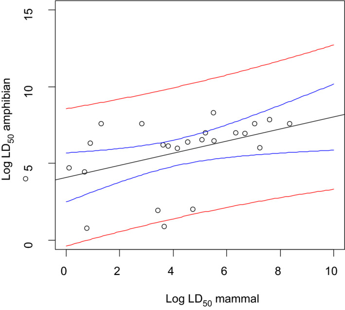
Comparison of amphibian and mammal acute LD 50 values based on the data set presented in Crane et al. (2016). The blue lines are the 95% confidence intervals for the regression mean and the red lines are the 95% prediction intervals. Log amphibian LD 50 = Log mammal LD 50 × 0.393 + 4.0899, R2 = 0.2144, p = 0.0227
Literature data were used to compare the toxicity endpoints for mammals and birds with endpoints for reptiles and terrestrial stages of amphibians (Ortiz‐Santaliestra et al., 2017). Only weak correlations between endpoints were found which never reached statistical significance. Based on the available data, it was not possible to extrapolate from endpoints observed in birds and mammals to amphibians and reptiles. The comparisons actually suggest that amphibian and reptile endpoints are rather complementary to the mammal and bird endpoints than correlated. For example some groups of compounds such as pyrethroids were systematically more toxic to amphibians and reptiles. This was also found by Weir et al., 2010.
One reason for the differences in sensitivity may be due to slower metabolisation and hence longer retention of toxic compounds in poikilothermic vertebrates. In addition, elimination rates of compounds may be slower in poikilothermic vertebrates. However, in contrast, slow metabolism may make poikilothermic animals less sensitive to compounds which become more toxic when metabolised (e.g. some organophosphate insecticides, Sanchez‐Hernandez and Walker, 2000).
The influence of homoiothermic and poikilothermic metabolism on toxicity of compounds with different properties should be investigated further. This could help to make recommendations on when surrogate endpoints from birds and mammals can be used and when testing with amphibians and reptiles is needed. It might even be possible to use amphibian and reptile endpoints as surrogates in the mammalian and bird risk assessment for some compounds. Eventually it would be possible to test amphibians and reptiles in a first tier for certain compounds and use their endpoints.
General considerations on coverage of endocrine and reproductive effects in amphibians and reptiles by birds and mammals
Amphibians have a unique phase in their life cycle with a complete transformation of the animal (metamorphosis) and therefore potential detrimental effects on metamorphosis in amphibians cannot be covered in bird or mammal reproductive toxicity studies.
In amphibians and reptiles, gonadal differentiation is affected by factors such as hormone levels or temperature in addition to the genetic mechanisms for determination of sex (see Section 2). Gonadal differentiation in reptiles and amphibians is therefore a plastic process that may be more susceptible to impact of endocrine‐disrupting chemicals than in birds and mammals. Reproductive toxicity studies in birds and mammals (such as OECD 416) include endpoints with potential information relating to identification of endocrine‐disrupting effect (oestrogen, androgen, thyroid). There is evidence showing that gonadal alterations observed after 17β estradiol exposure in the painted turtle (Chrysemys picta) were comparable to alterations observed in birds after in ovo exposure (Berg et al., 1999, 2001a), suggesting that endocrine‐disrupting chemicals may induce similar effects on gonadal differentiation in birds and reptiles. In principle, it might be possible to extrapolate certain effects from bird long‐term studies to effects on reptiles. Reproductive toxicity studies in birds (OECD 206) usually do not include thorough histopathological examination. This information would be highly valuable and serve as a good indicator of potential detrimental effects on gonadal/Müllerian duct differentiation and development in reptiles (Crain et al., 1999; Berg et al., 2001b). Critical routes of exposure at critical windows of development may not, however, be comparable in birds, mammals, reptiles and amphibians, which makes potential extrapolation of effects uncertain.
In vitro tests to detect endocrine effects are available for mammals (e.g. ER‐transactivation assay OECD 455, aromatase assay OECD (USEPA) and other tests are still being developed (e.g. androgen receptor transactivation assay). As already pointed out by EFSA (2013), mechanistic information on the endocrine pathways and availability of internationally standardised test methods is limited for amphibians and very limited for reptiles. Hence, it is unclear whether observations related to endocrine effects in the studies with mammals can be extrapolated to amphibians and reptiles. There is a need for specific tests and/or information on the endocrine pathway and susceptibility of amphibians and reptiles at various life stages, including in vitro data. Standard tests exist for amphibians to detect effects on the thyroid axis and development of sex organs (see Section 8) but they are lacking for reptiles.
General consideration on coverage of behavioural effects
The ongoing behaviour of non‐target species should be protected according to the EU regulation 1107/2009. The tests with birds and mammals do not systematically investigate behavioural effects. Some non‐standardised test with amphibians and reptiles exist (see Section 8). Further investigation is needed into how relevant behavioural effects observed under laboratory conditions are to wild populations.
General considerations on coverage of dermal toxicity
At present, the Bird and Mammal Guidance Document (EFSA 2009b) does not require any specific information with respect to inhalation and dermal toxicity and hence no surrogate endpoints are available for extrapolation to amphibians and reptiles. Dermal toxicity is currently investigated only for human risk assessment. It covers several aspects, including systemic toxicity via the dermal route of exposure, local effects as dermal irritation and skin sensitisation. For the estimation of the systemically available exposure levels in cases of non‐dietary exposure, the dermal absorption of the active ingredients as well as of the dilution(s) of the plant protection products is also measured for the establishment of the appropriate absorption factors for human risk assessment.
Coverage of amphibian and reptilian toxicity by routine rodent dermal (OECD 402, 410) and absorption ([Link], [Link]) tests may not be completely adequate, especially with respect to amphibians.
There is a general agreement on the high permeability of amphibian skin, being much higher than mammalian dermal absorption (Quaranta et al., 2009), (Kaufmann and Dohmen, 2016). Ex vivo skin‐absorption tests could be used to estimate adequate dermal absorption factors instead of default values (100%). Furthermore, amphibian skin plays an important role as a respiratory organ and some studies with pesticides clearly show that dermal exposure may be lethal, even without any systemic exposure, as a result of respiration defects (Johnson et al., 2017). Overall, the current dermal toxicity tests in rodents do not cover the specific risk for amphibians, while reptiles appear more similar to mammals (Weir et al., 2015, 2016c). This suggests that some methods used in assessing dermal exposure/toxicity in mammals may be applicable to reptiles and could be used as a surrogate. However, no direct investigations have been undertaken to investigate the relationship between mammal and reptile dermal exposure or toxicity. Mineau (2012) reported a strong relationship between mammal and avian dermal toxicity values for several pesticides, suggesting that a similar relationship may be built for reptiles and mammals, but data are currently lacking.
Testing for skin irritation in mammals, both in vitro (e.g. OECD 431) and in vivo (OECD 404), is probably appropriate for the estimation of the irritation potential of PPPs and active ingredients for amphibians and/or reptiles, considering that irritation is a mechanism of toxic response, which may occur in all vertebrate species. Skin irritation is commonly described as a result of toxicant exposure in amphibians (Pessier, 2002).
Skin‐irritation tests in mammalian species cannot, however, provide any information in relation to mucus‐layer degradation of amphibians, which may occur, and there are no published data evaluating chemical characteristics of toxicants that might lead to the degradation of the mucus layer. It is suspected that some chemicals may have a detrimental impact on this layer without being irritant (pyraclostrobin case study). Furthermore, surfactants, for instance, may have an important impact on the mucus layer in amphibians without any significant or strong irritation potential in mammals. In the case of reptiles, the skin structure appears to be similar to mammalian skin and dermal irritation tests (e.g. OECD 404 or 431) could cover this particular risk (Weir et al., 2015).
With respect to skin sensitisation, there is no evidence or data to support the applicability of tests to amphibians or reptiles.
Many studies show that dermal exposure may result in severe immunological disorders in amphibians and that this is not adequately covered by existing tests (Johnson et al., 2017). It is also demonstrated that exposure in the field may result in secondary bacterial or fungal contamination leading to delayed death (Pessier, 2002). Several authors have demonstrated that peptides present in skin secretions may have an important immune protective effect (Conlon et al., 2011). None of the existing tests cover this issue. A dermal overspray test would appear appropriate to estimate this kind of damage.
In conclusion, there is a need for adapted protocols to evaluate dermal toxicity, dermal absorption and indirect consequences of dermal exposure in amphibians and reptiles. Further research is warranted to establish appropriate protocols and endpoints for evaluation. This is especially needed for amphibian skin as it is too different in its anatomy and function from mammalian skin to exclude skin effects in amphibians even if there are no effects observed in tests with mammalian skin. Endpoints from skin tests to be used in a risk assessment context are skin lesion (irritation/corrosion) and dermal adsorption. Such a test could be used in a first‐tier screening. In order to minimise animal testing, it would be highly desirable to develop in vitro methods. For measuring skin permeability, a test design similar to the one in Kaufmann and Dohmen (2016) could be used. For skin irritation, it might be an option to develop a test for measuring skin irritation in amphibian keratinocyte cell cultures similar to OECD 439 and measuring viability of cells with an MMT assay. However, there would be uncertainty with regard to effects on the whole animal as there is no active uptake in vitro and not accounting for effects on respiratory function. Therefore, in vivo tests with amphibians would still be needed. Only if a scientific research project would generate enough test results with in vivo/in vitro outcomes for different types of pesticidal active substances and PPPs, then it could be looked into whether it is possible to extrapolate from the in vitro to in vivo effects. The results of such a research programme could also be used to set up and test TK/TD models for amphibians.
Influence of temperature on toxicity
Biological activity of amphibians and reptiles usually increases with higher temperatures (under temperate climates) because of poikilothermy. As a consequence, the FIR will increase, exposure will increase and toxicity may reach its peak. There is no direct relationship, however, between metabolic rates, FIR and external temperature (Harvey‐Pough, 1983). Enzyme activity may vary as a result of external temperature modifications. It has been shown, for instance, that cholinesterase activity is highly dependent of temperature, with increased basal activity in frogs raised at 19°C vs frogs raised at 8°C (Johnson et al., 2005). As a consequence, lower temperatures could be associated with increased susceptibility of amphibians or reptiles, as also commonly observed for pyrethrins (Talent, 2005; Weir et al., 2015) in lizards, glyphosate (formulated PPP) in common toads (Baier et al., 2016), or copper sulfate toxicity in amphibians (Chiari et al., 2015). This is not true for all active substances or commercial formulations, and other reports are available indicating a higher susceptibility of amphibians and reptiles to PPP active substances such as endosulfan (Broomhall, 2002), methomyl (Lau et al., 2015), carbaryl and malathion (Rumschlag et al., 2014) with increasing temperatures. There is also one published evidence of non‐monotonic response to an active substance (glyphosate) (Gandhi and Cecala, 2016). In a recent study in tropical frogs (Alza et al., 2016), temperature alone has a positive influence on tadpole growth, but chlorothalonil toxicity is not modified by changes in diurnal temperature (limited range of + 1–+ 9°C difference).
It is also important to mention the major role of external temperature on the egg development and gender determination in reptiles, which cannot be evaluated with current toxicological endpoints from birds, mammals or human toxicity studies. It has been shown, for instance, that very low environmental exposure of eggs to xenoestrogens such as DDT may lower the temperature threshold on sex determination in alligators (Milnes et al., 2005).
Overall, there are only limited data available to describe the relationship between temperature and toxicity in amphibians and reptiles, and there is no evidence of a general dose–response curve. It is impossible to predict the impact of temperature on the toxicity of a given PPP (either as an active substance or as a commercial product) in amphibians or reptiles. Furthermore, the current risk assessment in birds and mammals or human beings is not adapted to integrate ectothermy and its potential effects on toxicity or exposure and any extrapolation from birds, mammals or human risk assessment should include some evaluation of the potential influence of ectothermy.
Overall conclusion
The acute oral toxicity of pesticidally active substances to amphibians and reptiles might in theory be covered by studies with birds and mammals. This possibility is, however, uncertain because there are few data available, in terms of either substances or amphibian and reptile species tested. Any general conclusion on potential coverage and assessment factors would be highly uncertain. The main issues that need to be addressed are potential differences in species sensitivity and relevance of the different modes of action of pesticidally active substances in respect of differences in susceptibility between species. Correlation between endpoints from birds and mammals with endpoints from amphibians and reptiles is a prerequisite for extrapolation and using birds and mammal endpoints as surrogates in a risk assessment. Only weak correlations between endpoints were found. Analysis of available data by examination of substance groups based on mode of action suggests that the amphibian and reptile endpoints complement, but are not well‐predicted by, the mammal and bird endpoints. It is therefore not possible to extrapolate safely from endpoints observed in birds and mammals to amphibians and reptiles based on the limited data available.
Even greater uncertainty exists regarding potential coverage of long‐term toxicity. For example, detrimental effects on amphibian metamorphosis are not covered. It might be possible to use effects observed in bird‐reprodution studies (with some modifications of the test protocol, e.g. adding histopathological observations) in the risk assessment for reptiles.
Amphibians and reptiles are poikilothermic and therefore have lower metabolic rates compared to birds and mammals. Ambient temperature is an important factor modifying toxicity in poikilothermic animals. In case that metabolic activation of a substance leads to increased toxicity (e.g. anticoagulants), then amphibians and reptiles may react less sensitively or with delayed effects compared to birds and mammals because of their slower metabolism. If initial metabolism reduces toxicity of a pesticidally active substance, then fast metabolisers such as birds and mammals will react less sensitively. In this case, temperature will have strong effects on the toxicity of the compound to amphibians and reptiles with enhanced toxicity at lower temperatures. Therefore, the specific mode of action of a pesticidal active substance and the interplay between metabolic rates and temperature need to be taken into account when using birds and mammal toxicity data as surrogates.
Coverage of endocrine effects in amphibians and reptiles by available studies with birds and mammals is uncertain because critical routes of exposure and critical windows of development may be different. Specific test protocols exist for amphibians but are lacking for reptiles. It needs to be investigated further whether endocrine effects on reptiles are covered by mammals and birds.
Dermal toxicity and adsorption data from mammals may be used as surrogates for reptiles but not for amphibians. Amphibian skin has important functions such as respiration, water regulation and immune function. The structure of amphibian skin with its mucus layer is very different from mammalian skin and therefore it is not possible to extrapolate to effects on amphibians. A test to investigate local effects on amphibian skin is needed. Systemic effects from dermal exposure also need to be addressed. Ideally, such tests should be in vitro studies to avoid animal testing. The WG recommends developing in vitro tests with amphibian skin for inclusion in future risk assessment schemes.
10.3.2. Potential coverage of the exposure assessment – analysis of available existing exposure models for birds, non‐human mammals and humans, and suitability for amphibians and reptiles exposure assessment for oral uptake
Oral exposure
Oral exposure via food uptake
The risk assessment of birds and mammals considers oral uptake of contaminated food items and drinking water. In addition, there is a risk assessment for bioaccumulation and food chain behaviour focused on earthworm and fish eating birds (see Annexes D and E for details on the current risk assessment for birds and mammals).
Residues in different food items, percentage of contaminated food in the diet and food uptake rates determine the oral exposure. All three parameters need to be considered when comparing oral exposure across taxa. Provided that the same food items are consumed and 100% contaminated food is consumed, then the comparison of food‐intake rates provide an indication of differences in oral exposure.
The Table 42 below compares food intake rates from birds, herbivorous mammals and herbivorous and insectivorous reptiles.
Table 42.
| Group | FIR (100 g animal) |
|---|---|
| Birds – passerines | 19.94 |
| Birds – non‐passerines | 9.56 |
| Seabirds | 12.66 |
| Rodents | 8.33 |
| Herbivores | 16.41 |
| Iguanid‐Herbivore | 0.91 |
| Iguanid‐Insectivore | 0.45 |
Food intake rates (FIR) are greater for birds and mammals than for amphibians and reptiles, by at least one order of magnitude (USEPA, 1993). Specific FIR equations are used by the USEPA in order to adapt their exposure model from birds to reptiles or amphibians.
Field metabolic rates of birds and mammals are about 12–20 times higher than for equally sized reptiles (Nagy, 2005) (Figure 39). Therefore, it is concluded that the oral exposure estimates for birds and mammals would result in a conservative estimate of oral exposure of amphibians and reptiles.
Figure 39.
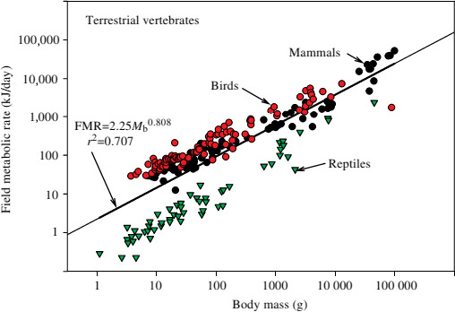
Field metabolic rates for birds, mammals and reptiles (from Nagy, 2005)
On the basis of FIR comparison, it can be concluded that the exposure assessment of secondary poisoning for earthworm‐ and fish‐eating birds and mammals will cover amphibians and reptiles with a similar diet. However, some reptiles are specialised predators and some snake species feed mainly on rodents. Snakes can access the burrows where baits are put and where rodents can be found. In addition, poisoned rodents may be more prone to predation (Cox and Smith, 1992). Therefore, it is likely that snakes can be exposed via secondary poisoning by rodents. Snakes can take up in one meal much more relative to their body size than a predatory bird or mammal. Therefore, it is unlikely that exposure estimates for predatory birds and mammals would cover snakes. It is proposed that a risk assessment for snakes is conducted for rodenticides.
Comparison of oral exposure of amphibians, reptiles and birds and mammals based on worst‐case assumptions and species specific food intake rates can be found in Appendix G. The calculations confirm that birds and mammals have a greater oral exposure than amphibians and reptiles. Hence the screening and first‐tier exposure assessment for insectivorous and herbivorous birds and mammals would most likely cover amphibians and reptiles.
Furthermore, the comparisons show that insectivorous lizards have a similar oral exposure to insectivorous amphibians and that herbivorous reptiles (tortoise) have a greater oral exposure than insectivorous reptiles. The estimated oral exposure of snakes from consumption of an oversprayed frog is slightly greater than the oral exposure of insectivorous lizards and amphibians and it is slightly below the oral exposure of tortoise.
An oral‐exposure, risk‐assessment method for amphibians and reptiles (T‐herps) was developed by the USEPA. For a detailed review, please see Appendix G. The model also includes prey items such as small mammals (rodents) and amphibians. The T‐herps model could be used as a risk assessment tool after adjusting it to model European species (such as the crested newt or Natrix natrix) for adapted FIR.
Oral exposure via water uptake
Exposure via drinking water depends on the concentration of pesticidal active substances in the sources of water and the water demand of the animals. The standard risk assessment for birds and mammals considers two sources
Puddles in the field
Water in leaf axils of crops
The exposure assessment is based on 100% uptake of water from these sources. For details on the risk assessment for birds and mammals from uptake of contaminated drinking water see Annex G.
It is unlikely that amphibians and reptiles would use water sources with higher concentrations of pesticidal active substances. Therefore, whether the exposure estimates for birds and mammal cover also amphibians and reptiles depends on the daily water requirements for amphibians and reptiles.
Amphibians take up water via their skin and hence this exposure route will be covered by a dermal exposure assessment. Reptiles take up water orally to satisfy their water demand. A first‐tier calculation for water uptake was conducted for lizards based on the allometric equation in Fryday and Thompson, 2009 (see Appendix G for details). The drinking water demand for a medium sized lizard (11 g) was calculated as 0.049 L/kg bw per day. This is about 10 times and about 5 times lower than the drinking water demand of 0.46 L/kg bw per day and 0.24 L/kg bw per day for a small granivorous bird (15.3 g) and small granivorous mammal (21.7 g), which are the bases for calculating drinking water exposure in EFSA, 2009 (Birds and Mammals GD). Therefore, it can be concluded that the estimate for drinking water uptake for birds and mammals would cover the water uptake of lizards.
If the drinking water uptake for birds and mammals is refined in the risk assessment, then the exposure estimate may not cover lizards any longer. Uncertainty remains with regard to other groups of reptiles such as snakes and tortoise because no information was available for calculating the water demands. This should be investigated further in order to draw conclusions on the coverage of snakes and tortoises by the existing exposure estimates for water uptake in birds and mammals.
Oral exposure from granular formulations and treated seeds
Ingestion of granules as food, grit or accidental uptake (mistaken as food) and residues of applications in food items is evaluated for birds and mammals.
If there is a possibility that granules are mistaken as food items, then the same assessment procedure applies as for contaminated food items (e.g. from overspray). The same conclusions with regard to coverage of amphibians and reptiles as above for uptake of contaminated food items can be drawn (i.e. amphibians and reptiles are covered by existing exposure estimates).
There is no evidence that amphibians and reptiles take up grit intentionally. European amphibians and reptiles do not have muscular gizzards. Therefore, this exposure is most likely not relevant.
There may be accidental ingestion of granules when eating food contaminated with soil. It is unknown how much soil amphibians and reptiles take up when feeding and whether it is different from birds and mammals. If the amount of soil taken up per food item is similar, then the exposure estimates from soil uptake of birds and mammals will cover amphibians and reptiles as well since they have lower food‐intake rates and hence feed less.
Dermal and inhalation exposure
The risk from dermal and inhalation exposure is not included in the risk assessment for birds and mammals in Europe. However, dermal and inhalation exposure models for birds were developed by the USEPA (Terrestrial Investigation Model, TIM). Dermal and inhalation exposure models also exist for human risk assessment. A review of the potential use of different exposure models can be found in Appendix H.
The dermal exposure model from the USEPA for birds could provide a basis for suggesting an exposure model for amphibians and reptiles. However, it would be necessary to use amphibian and reptile specific factors such as dermal absorption fraction (DAF), the surface area of the animal and foliar contact rate.
For example, for birds, it is assumed that only the feet have direct contact to foliage while for amphibians and reptiles the full surface area could come in contact with foliar residues. It may be possible to refine this assumption if data from contact surface of the animal with different crop types become available, e.g. the sides of the animal are in contact with vegetation and the ventral side is in contact with crops where animals can climb (e.g. orchards).
A default factor for foliar contact rate is applied in TIM. This factor would need to be adjusted for amphibians and reptiles. Such a factor could be derived from information on the speed of movement and surface area of the animal in contact with foliage during movement.
The dermal route equivalency factor is applied to estimated dermal exposures in order to derive an estimate of the equivalent oral dose. It is not expected that oral toxicity and dermal toxicity data are available for amphibians and reptiles. This constitutes a problem for adding up the exposures and comparing them to one endpoint (either dermal or oral LD50). Whether the dermal route equivalency factor for mammals or birds could be extrapolated to amphibians and reptiles is highly uncertain. Because of the specific functions of amphibian skin for gas exchange and water regulation, it is expected that amphibians will be more sensitive to dermal exposure than birds or mammals.
The following is needed in order to address dermal exposure from contact to residues in soil and plants:
An estimate of the body surface of amphibians and reptiles in contact with soil and plants while moving.
Dermal absorption factors for amphibians and reptiles
How much of the residues in soil and plants can be translocated to the amphibian and reptile skin
Speed of movement
Time of when they are actively moving vs resting.
A possible method to calculate exposure from overspray is included in Appendix G. The calculations were conducted with worst‐case assumptions such as direct overspray of animals and 100% dermal absorption in both groups of amphibians and reptiles. The main differences in dermal exposure are therefore related to differences in the shape of their bodies.
The dermal exposure from overspray is greater for reptiles than for amphibians with equal weights. Lizards and snakes have similar dermal exposure because of the similarities in their shape and hence surface area to volume ratio.
For amphibians, the dermal exposure from overspray is comparable to the daily dietary dose while for lizards and snakes the dermal exposure from overspray is about one order of magnitude greater than the daily dietary exposure from oral uptake.
The dermal exposure from overspray is lower for amphibians compared to the daily dietary dose of birds and mammals. The dermal exposure for reptiles (lizards and snakes) is in the same range as the daily dietary dose for birds and mammals. However, sensitivity to different routes of exposure may be different and hence no conclusion can be drawn with regard to coverage of risk.
Ventilation rates and oxygen consumption of different reptile groups and birds and mammals were compared by Bennett (1973). Higher ventilation rates of homeotherms are principally the result of a greater ventilation frequency in mammals and a greater tidal volume in birds. The inhaled volume of air per minute is about 3.6 times and 4.9 times greater in birds and mammals compared to reptiles. Therefore, it is expected that the contribution of inhalation exposure to the total exposure is much less than oral and dermal exposure and it is not considered necessary to assess inhalation exposure by default. However, an inhalation exposure assessment may be needed if a substance is volatile and very toxic to reptiles. Inhaled volumes in amphibians are likely to be even less than for reptiles as their skin has an important function for gas exchange. Therefore, it is not considered necessary to conduct an inhalation exposure assessment for amphibians.
The Potential Dermal Exposure (PDE) equation, used for the first‐tier potential dermal exposure estimation for workers could be applied for the PDE estimates of amphibians and reptiles. More specifically, the dislodgeable foliar residue (DFR) values 3 μg active substance/cm2 of foliage/kg a.s. applied/ha could be used as a first‐tier assessment. Furthermore, the transfer coefficient (TC) could be estimated on the basis of the fraction of the total body area of the organism(s) and its activity (contact duration with new surfaces per hour) assuming that it is in continuous contact with the treated crop for a number of hours (T). The time will depend on the behaviour of the animal and it will be estimated from the time spent in the treated crop or in the contaminated field. Furthermore, for multiple applications the MAF could be considered. If this approach is applied, the following parameters need to be identified for the most relevant life stage of the organism:
Toxicological endpoint (TEP) and the respective threshold (NOAEL and Acceptable level of dermal exposure).
The assessment factor for the conversion of the NOAEL to the toxicological threshold,
If the TEP will be derived from a study carried out via the dermal route of exposure, no dermal absorption factor is needed. In this case the acceptable dermal exposure (Regulatory threshold for acceptable exposure = NOAELdermal/assessment factor) can be directly compared to dermal exposure (DE). However, if it is derived from oral exposure (Regulatory threshold for acceptable exposure = NOAELoral/assessment factor), information on both oral and dermal absorption (DA) is necessary [oral absorption for correction of the oral dose in order to get the systemic threshold and the dermal absorption for the estimation of the systemic dermal exposure (SDE) from the dermal exposure (SDE = DE × DA)]
Body surface area in contact with the foliage,
Behaviour of the animal and time spent in the treated field.
10.4. Conclusions on the coverage by the current risk assessment
10.4.1. Overall conclusions for aquatic life stages by the current risk assessments in the aquatic risk assessment
Apart from accurately predicting the toxicity and exposure, assessment factors need to be defined in order to evaluate the risks to amphibians and reptiles from pesticides. The assessment factors should cover the uncertainties in the risk assessment, which are described in Section 7.11.
Based on the above we conclude the following for amphibians in their aquatic environment:
Endpoints derived in acute toxicity testing with fish are considered sufficiently accurate to predict the acute toxicity for aquatic life stages of amphibians if an extrapolation factor will be included to achieve a higher proportion (> 70%) of cases covered by the acute endpoint for fish. The magnitude of an additional assessment factor should be calculated after agreement on the proportion of amphibian response data to be covered by the fish acute endpoints. From available data, it seems that the aquatic RAC covers the amphibian (aquatic life stages) sensitivity. For extrapolation to amphibian toxicity, it is suggested to use the fish endpoint because a correlation in toxicity was observed. However, the extrapolation from fish to amphibian endpoints is only applicable for the first‐tier risk assessment.
In order to assess the chronic toxicity to aquatic life stages of amphibians, an extended life cycle test based on LAGDA test should be conducted in order to address effects on metamorphosis and reproduction, which are not adequately addressed by the chronic studies with fish. Sensitive and relevant endpoints to assess populations in the field considering habits and behaviour of the biphasic species after multiple exposures need to be defined
With regard to the exposure assessment by FOCUS step 3, the Working Group is unable to predict whether the acute exposure will be conservative for amphibians in their aquatic environment. The most vulnerable 10% amphibian ponds are smaller in size and shallower than FOCUS ponds, so concentrations in FOCUS ponds are expected to be non‐conservative for amphibian ponds. For FOCUS streams and ditches, it is not possible to predict a priori whether their acute exposure concentrations will be conservative or not but, due to their high flow‐through rate compared to the one in FOCUS ponds, their chronic exposure concentrations are expected to be non‐conservative.
The sediment‐exposure assessment by the FOCUS surface water step 3 scenarios is expected not to represent realistic worst‐case exposure situations. The FOCUS surface water step 3 scenarios were designed to represent realistic worst‐case exposure situations for the PECs in water. Due to the partition between water and sediment, high concentrations in the water layer are associated to low concentrations in the sediment. Moreover, for slowly degrading and/or sorbing pesticides, accumulation of pesticides over the years is important and the FOCUS scenarios cannot account for this as they simulate only one year.
The suitability of the current assessment factors used in the first tier to cover the uncertainties for amphibians and reptiles need to be evaluated.
10.4.2. Overall conclusions with regard to coverage of amphibians and reptiles by existing risk assessments for birds, mammals and humans
No general conclusion can be drawn on whether the acute oral toxicity of pesticidally active substances is covered by studies with birds and mammals because data sources are scarce. The main issues that need to be addressed are potential differences in species sensitivity and relevance of coverage of the different modes of action of pesticidally active substances in respect of the different susceptibility between species. Even greater uncertainty exists regarding potential coverage of long‐term toxicity. For example, detrimental effects on amphibian metamorphosis are not covered. It might be possible to use effects observed in bird‐reproduction studies (with some modifications of the test protocol e.g. adding histopathological observations) in the risk assessment for reptiles.
Amphibians and reptiles are poikilothermic and therefore have lower metabolic rates compared to birds and mammals. Ambient temperature is an important factor modifying toxicity in poikilothermic animals. The specific mode of action of a pesticidally active substance and the interplay between metabolic rates and temperature need to be taken into account when using bird and mammal toxicity data as surrogates.
Coverage of endocrine effects in amphibians and reptiles by available studies with birds and mammals is uncertain because sensitive life stages, critical routes of exposure and critical windows of development may be different. Specific test protocols exist for amphibians but are lacking for reptiles. It needs to be investigated further if endocrine effects on reptiles are covered by mammals and birds.
Dermal toxicity and adsorption data from mammals may be used as surrogates for reptiles but not for amphibians. Specific attention should be paid to dermal exposure and its direct and indirect effects in amphibians (impact of exposure on the mucus layer and consequence of the health status of the individual). Amphibian skin has important functions such as respiration, water regulation and immune function. The structure of amphibian skin with its mucus layer is very different from mammalian skin and therefore it is not possible to extrapolate to effects on amphibians. A test to investigate local effects on amphibian skin is needed. Systemic effects from dermal exposure also need to be addressed. Ideally such tests should be in vitro studies to avoid animal testing. The WG recommends developing in vitro tests with amphibian skin for inclusion in future risk assessment schemes.
The oral exposure estimates from the screening steps in the risk assessment for birds and mammals may cover the risk to amphibians (depending on the toxicological sensitivity and assessment factors that are applied).
The dermal exposure estimates for lizards and snakes are in the same range as the daily dietary exposure estimates for birds and mammals. The risk from dermal exposure is not assessed for birds and mammals. Therefore coverage of reptiles by the risk assessment for birds and mammals is highly uncertain.
The comparisons of the daily dietary exposure and dermal exposure from overspray give an indication that both exposure pathways are of high importance and both need to be considered in the risk assessment for amphibians and reptiles.
Coverage of amphibians and reptiles by human risk assessment could be considered as a 1st step, with appropriate exposure factors (body surface area in contact with foliage, behaviour and time spent in the treated field). Overall, coverage by human risk assessment may be highly uncertain because of lack of an appropriate toxicity endpoint.
11. Conclusions
Overall, the Panel concludes that several species of amphibians and reptiles occur in agricultural landscapes where they are exposed to PPP, and this exposure may have unacceptable consequences on individuals and populations. Therefore, a specific environmental risk assessment scheme is needed for both amphibians and reptiles.
11.1.
11.1.1.
General risk‐assessment considerations related to the biology of amphibians and reptiles
Although traditionally studied together under the discipline of herpetology, amphibians and reptiles present important differences in many of their biological and ecological features. What differentiates them from birds or mammals is that they are poikilothermic. Sensitivity and exposure to pesticides, affected by poikilothermy through its influence on physiology, growth, development, behaviour or reproduction may be shared, but other factors, e.g. skin permeability in amphibians, may also have a large influence on risks associated with PPPs.
The presence of amphibians and reptiles in agricultural areas, both in‐field and on the edge of the field, is well documented. Potential for overspray, dermal exposure by contact with soils or plants during or following PPP applications, and oral uptake of pesticides through ingestion of contaminated materials exist for both groups. Exposure of amphibians and reptiles when inhabiting a treated area can be prolonged, especially in the case of the most territorial reptile species or of the amphibian aquatic life stages.
The potential of surrogate‐based risk assessment to cover toxicity of pesticides on amphibians and reptiles by other vertebrate groups is compromised by some particular biological processes typical of these animals, including metamorphosis in amphibians or hormonal‐dependent sex determination in both amphibians and reptiles. Also, the peculiarity of the amphibian life cycle compared to other vertebrate groups has a major influence on potential exposure scenarios, which is difficult to predict from data generated from other taxa. When compared to fish, amphibians possess some structures typical of higher vertebrates that do not occur in fish (e.g. the Müllerian ducts that are precursors of sexual organs). Impacts of pesticides on these structures cannot be identified through fish‐based evaluations and require assessment at specific, sensitive time windows within the amphibian aquatic development.
Amphibians and reptiles are two very diverse groups. This diversity has been considered in the definition of functional groups for assessment, based not only on taxonomic differences but also in large ecological differences within the same main taxonomic group. From the identified groups, potential focal species are proposed on the basis of traits related to pesticide exposure and potential to exert toxicity.
For individual amphibians and reptiles, exposure to PPPs can take place differentially in space and time, depending upon the behaviour of the animals coincident with PPP availability in the environment. Therefore, realistic risk assessments should take spatial behaviour within a season into account. This is particularly important for migrating amphibians.
Population structure and spatio‐temporal dynamics can have important implications for the evaluation of impacts of PPP on amphibian and reptile populations. Therefore, for inclusion of both spatial and temporal implications of PPP usage, and to take the ecological state of the population before application of PPPs into account, a systems approach is recommended (EFSA Scientific Committee, 2016a).
Spatially explicit individual‐based modelling at landscape scales is an important part of the ERA toolbox for amphibians and reptiles. It should be used to help set the tolerable magnitude of effects for specific protection goals (SPG), to translate toxicity data to population modelling endpoints, and as a higher tier assessment tool.
Precise context for application of the models requires careful consideration. The regulatory scenarios need to consider all factors; in particular, landscape structure and weather have a large impact on the outcome of the long‐term risk assessment.
Conclusions on protection goals and general risk assessment framework
The Panel proposes SPG options to be considered in the risk assessment of amphibians and reptiles exposed to PPPs. These SPG options were derived based on (i) the legislative requirements in place for non‐target vertebrates, (ii) the need to encompass the endangered status of a great proportion of amphibian and reptile species, and (iii) the importance of amphibians and reptiles as drivers of valuable ecosystem services in agricultural landscapes.
The key drivers (or service providing units, SPUs) identified among amphibians are Anura (frogs and toads) and Caudata (newts and salamanders); for reptiles, sauria (lizards, skinks and geckos), Ophidia (snakes) and – within the Testudines – terrestrial and freshwater turtles.
Amphibians and reptiles are key drivers of the following ecosystem services: provision of genetic resources and biodiversity, maintenance of cultural services, provision of food and pharmaceutical resources, support of nutrient cycling and soil structure formation, regulation of pest and disease outbreak and invasion resistance, and the support of food webs in agricultural landscapes.
The Panel does not consider it appropriate to define SPG options on the basis of functional groups of amphibians and reptiles. In order to protect these significantly endangered vertebrate groups, the ecological entities to be protected are the individuals and populations of species.
It is proposed to set SPG options on the individual level for the survival of adult amphibians and reptiles. In addition, the long‐term persistence of populations should be considered. Attributes of population persistence relate to the assessment of abundance/biomass of amphibian and reptile species and also to the landscape occupancy of these species, and to changes in population growth rates. Giving the mobility of most amphibian and reptile species, no separate SPG options are proposed for in‐field and off‐field areas.
The need to assess the risk for these non‐target vertebrate species when exposed to PPPs faces a paucity of standardised testing methodologies and comprehensive data sets on their toxicological sensitivity to (active substances in) PPPs. The Panel proposes to require ecotoxicological data for a limited period of time and to review the evidence after some time in order to decide on possible waiving of tests in future.
Data are needed on the chronic toxicity of PPPs for amphibians, starting from the exposure in the aquatic stages up to and including the adult stages. Data are also needed on the effects of PPP on amphibian terrestrial stages via the dermal route of exposure (overspray, contact with plants and soil).
Toxicological endpoints related to certain aspects of amphibian biology, like metamorphosis or hormone‐dependent sex determination, cannot be predicted from information generated from surrogate taxa. Similar concerns apply to reptiles. A specific approach to investigate chronic toxicity leading to effects on these aspects is required.
Variability in sensitivity throughout the life cycle is also translated in the existence of key moments at which certain effects are more likely to happen. This must be considered when short‐term toxicity is assessed. For instance, maturation of sexual organs has a tightly defined time window, and testing reproductive toxicity of pesticides outside this window could lead to wrong assumptions about lack of effects.
Given the scarcity of data, it is not possible to conclude that toxicity data or existing risk‐assessment schemes with other non‐target vertebrates or other organism groups cover the acute and/or chronic risk of intended PPP uses to reptiles. Given the scarcity of information, it is also not possible for the time being to request specific tests to close these data gap.
The Panel proposes to follow a tiered approach for the risk assessment of amphibians and reptiles comprising an evaluation of effects at local and long‐term effects at the landscape scale.
At local scale, a risk assessment is required for all relevant environmental compartments in which different life‐stages live. For amphibians, this means that an evaluation of risk in the aquatic and in the terrestrial compartment is needed. This is not the case for reptiles.
Given the importance of different exposure routes, it will be necessary to assess the impact of PPPs on amphibians and reptiles resulting from a combination of the main exposure routes. In a first assessment step, it is suggested to address the outcome of exposure to PPPs through several routes by assessing the combined risks of the main routes.
After an assessment of effects at local scale, the risks of intended uses of PPP have to be assessed at landscape scale. This should be performed in a first step using prerun population models that address the long‐term repercussions of year‐on‐year PPP use on amphibians and reptiles.
It will be necessary to satisfy the risk‐assessment criteria at both local and landscape scales in order to conclude that SPGs set for amphibians or reptiles are met.
Conclusions on exposure considerations
The use of Exposure Assessment Goals defining the spatial unit with its EREQs and exposure routes allows for an explicit and systematic methodology to calculate PECs in the field for reptiles, as well for amphibians in their aquatic and terrestrial environment.
For amphibians and reptiles, no standard ecotoxicological experiments are required in the current pesticide‐registration procedure. Therefore, it is not yet possible to make a final choice on the EREQs that enable a coherent linking between exposure in the field and the endpoints of ecotoxicological experiments. This implies that all EREQs in this opinion are proposals, which may need to be changed later on.
For amphibians in the aquatic environment, exposure via dermal contact with pond water is judged to be more important than exposure via food intake. The main entry routes for pesticides into ponds in agricultural areas are spray‐drift deposition, run‐off or drainage. Sediment may accumulate pesticide residues and in such cases exposure of tadpoles by uptake of sediment may be an important route. In their terrestrial environment, dermal exposure is an important route for amphibians, especially by contact, e.g. with recently deposited pesticides on soil or plants, or in puddles within agricultural field. Overspray or spray‐drift deposition might occur. Intake of residues via food is another potential exposure route.
For reptiles, main exposure routes are via food intake, contact with residues in soil and plants and contact of eggs with contaminated soil. As many reptile species have a high site fidelity, dermal uptake may be important for reptiles living in and near agricultural fields, although their skin is less permeable than the skin of amphibians.
The analysis of the dimensions of the Spanish and Swiss amphibian ponds and the ponds in the UK demonstrated that the most vulnerable 10% are significantly smaller than the FOCUS ponds, used at present in the EU registration procedure. Therefore, it is expected that the FOCUS ponds do not deliver conservative exposure estimates for amphibian ponds. For peak concentrations in FOCUS ditches and streams, the Working Group was unable to make a general statement on conservativeness, but for chronic exposure FOCUS ditches and streams are expected to be non‐conservative, due to their relatively rapid flow‐through rates.
The FOCUS surface water step 3 scenarios are expected to result in non‐conservative exposure estimates for the sediment, as on the one hand they were designed to represent realistic worst‐case exposure situations for the PECs in water (generally associated with low sediment concentrations due to the partition between water and sediment) and on the other hand they do not account for multiyear accumulation in the sediment due to their simulations lasting only one year.
Conclusions on oral, dermal and inhalation exposure for different groups of amphibians and reptiles
The dermal exposure levels from overspray (assuming that half of the body surface receives the full application rate and 100% dermal uptake) is estimated to be greater for reptiles than for amphibians with equal weights and assuming the same skin permeability. However, reptile skin has lower absorption rates compared to amphibians. Lizards and snakes are expected to receive similar levels of dermal exposure under the same exposure scenario (because of the similarities in their shape and hence surface area to volume ratio).
For amphibians in the terrestrial environment, the dermal exposure from overspray is comparable to the daily dietary exposure.
For lizards, the dermal exposure from overspray is about one order of magnitude greater than the daily dietary exposure – given the same assumption as above on dermal uptake.
The dermal exposure from overspray is lower for amphibians compared to the daily dietary exposure of birds and mammals. However, the exposure level for reptiles is in the same range as the daily dietary exposure for birds and mammals.
Preliminary conclusions with regard to potential coverage of amphibians and reptiles in current risk assessment schemes for aquatic organisms, birds, mammals and human risk assessment
Available studies with fish assess the acute mortality and long‐term effects on appearance, size, behaviour and reproduction. Several studies were found in the literature indicating that the acute endpoints for amphibians (tadpoles) are lower than the acute endpoint for fish (mainly rainbow trout). This was the case for 30% of the assessed data points. Therefore, if a higher percentage of all amphibian mortality data points should be covered, an extrapolation factor needs to be applied on the acute fish endpoint to deliver an appropriate toxicity endpoint for the acute risk assessment of amphibians.
Two review studies were found comparing chronic endpoints for fish and amphibians. However, one study showed shortcomings in the methodologies as neither duration of study nor type of effects nor specification of concentration were comparable. In the other study, amphibians were more sensitive than fish in around 50% of the cases. Therefore, no conclusion can be drawn for the coverage of the chronic sensitivity by fish for amphibian species. Furthermore, the chronic fish studies do not adequately address relevant sublethal endpoints considered relevant for amphibians, such as effects on metamorphosis, reproduction or immunosuppression. No data (thus no comparison in toxicity) were found for reptiles in aquatic environments.
Shortcomings of the current toxicity comparisons are that (i) for a rather limited number of substances and life stages only the endpoints and not the slopes of the dose‐response curve were compared, (ii) the majority of amphibian studies were conducted with X. laevis, for which limited information is available with regard to its representativeness for European species and (iii) the variability between amphibian species is unknown, leaving it open which assessment factor adequately addresses the uncertainties stemming from the effect assessment.
In the aquatic system, amphibians as well as certain reptiles (water dwelling snakes and terrapins) may be exposed dermally to water and sediment or orally to feed and drinking water. Furthermore, eggs may be exposed by maternal transfer. The studies with fish adequately address the dermal exposure via water and the study with Lumbriculus the exposure via sediment. Therefore, further data about these habitats in the member states needs to be gathered. There is currently a lack of chemical monitoring data of aquatic amphibian habitats (especially small and standing water bodies) in Europe.
The oral exposure estimates from the screening steps in the risk assessment for birds and mammals may cover the exposure estimate for oral uptake of PPP residues to amphibians.
The dermal exposure estimates for lizards and snakes are in the same range as the daily dietary exposure estimates for birds and mammals. The risk from dermal exposure is not assessed for birds and mammals. Therefore, coverage of reptiles by the risk assessment for birds and mammals is highly uncertain.
The comparisons of the daily dietary exposure and dermal exposure from overspray give an indication that both exposure pathways are of high importance for amphibians and reptiles.
Whether the risk to amphibians and reptiles via oral uptake of PPP residues with food is covered by the risk assessment of birds and mammals depends on the differences in toxicological sensitivity and assessment factors applied.
Differences in sensitivity among life stages, especially within amphibians, because of the morphological and physiological differences among them, should be considered when determining the toxicity of pesticides.
Some standard tests are available for amphibians. These are LAGDA, AMA and FETAX. These tests do not cover the reproductive phase of amphibians. A full life cycle test with amphibians (e.g. with X. tropicalis) could be very useful in a risk‐assessment context because it enables the observation of reproductive effects.
No standard test guidelines exist for reptiles. In addition, very few data obtained from non‐standard tests are available. This lack of data makes it very difficult to compare the toxicological sensitivity among different reptile species and other groups of vertebrates and hence impossible to propose endpoints from surrogate species (e.g. birds) and assessment factors.
Sources of uncertainties in the current risk assessment have been identified, which need to be quantified for the calibration of a risk assessment scheme for amphibians and reptiles. Uncertainties were identified in the effect as well as exposure assessment.
12. Recommendations
The choice of potential focal species that can be also suitable to develop population models to support SPGs must be based on traits leading to potential exposure and sensitivity to pesticides.
-
Landscape‐scale spatially explicit mechanistic models for the six species identified as potential focal species for the assessment of amphibians and reptiles need to be developed and tested. These should include:
-
1
— mechanistic modelling of dispersal, reproduction and mortality factors for all life stages;
-
2
— the potential to introduce a wide range of impacts of PPPs in terms of modes of action, exposure and regulatory scenarios;
-
3
— spatial and temporal representation of resource distributions;
-
4
— realistic pesticide‐exposure modules including realistic or agreed methods to implement pesticide concentrations in ponds;
-
5
— exposure routes linking environmental concentration to the body‐burden of pesticide need to be defined and included, as well as inclusion of a suitable representation of multiple exposure events for an individual. The development of TK/TD models for amphibians and reptiles could help to address this issue.
-
1
Population modelling endpoints should include the abundance of the animals, their distribution and relative change in population growth rate as a result of application of the PPP. The latter takes into account long‐term impacts which can be difficult or impossible to see using other approaches.
The threshold limits of changes to population level endpoints that correspond to unacceptable impacts on the SPG need to be identified. This should not be done on an individual endpoint basis but combining abundance, occupancy and changes in growth rate.
There is a need to develop suitable refinement for the combination of exposure routes. If a risk is identified by a lower tier assessment by the addition of exposure routes, then a potential refinement might be possible if it can be shown that different routes are not additive. However, this would need to be supported by experimental data.
The Panel recommends the review of available data on amphibians and reptiles after an appropriate time frame in order to decide whether initial triggers flagging high/low risk for (active substance in) PPP can be set. The aim is to identify (active substances in) PPP for which requirements on toxicity data on amphibian may be waived. Owing to scarcity of data, this is not possible for the time being.
For chronic risk assessment of the aquatic stages of amphibians, the current exposure assessment via FOCUS step 3 scenarios may not be protective. For the acute risk assessment, this needs to be investigated further.
The FOCUS surface water scenarios (step 3) were not designed to give a protective exposure in sediment and hence are not recommended to be used in the risk assessment for sediment exposure of amphibians.
Chemical monitoring should be encouraged especially in small standing surface waters.
As dermal exposure is a main exposure route for amphibians in their terrestrial environment, the Panel recommends carrying out experiments that allow for the quantification of the amount of substance taken up by the animals including the identification of differences in skin permeability of the different body parts of the animal.
Acute toxicity tests with fish are considered sufficiently accurate to predict the acute toxicity for aquatic life stages of amphibians if an extrapolation factor will be included to achieve a higher proportion (> 70%) of cases covered by the acute endpoint for fish. The magnitude of an additional assessment factor should be calculated after agreement on the proportion of amphibian response data to be covered by the fish acute endpoints. If endpoints from other surrogate species (aquatic invertebrates or aquatic plants) are considered, a higher coverage of the sensitivity is achieved. However, this is only applicable for the first‐tier risk assessment.
To assess the chronic toxicity to aquatic life stages of amphibians, an extended life cycle test based on LAGDA test should be conducted in order to address effects on metamorphosis and reproduction, which are not adequately addressed by the chronic studies with fish.
Sensitive and relevant endpoints to assess populations in the field considering habits and behaviour of the biphasic species after multiple exposures need to be defined.
Sources of uncertainties in the current risk assessment, which have been identified, need to be addressed to calibrate a risk assessment scheme for amphibians and reptiles.
Oral and dermal exposure need to be considered in the risk assessment for terrestrial life stages of amphibians and reptiles. Inhalation exposure seems to be less relevant and hence development of inhalation‐exposure models has lower priority. If further information becomes available indicating that inhalation exposure is a relevant route of exposure, then it would be an option to adapt either the human inhalation‐exposure approach or the US‐EPA TIM model for birds to estimate inhalation exposure for amphibians and reptiles.
Currently, oral exposure in the bird and mammal guidance to assess the risk by intake of contaminated food relies on focal species and considers herbivores, insectivores and granivorous. The food intake rate of amphibians and reptiles is generally lower. Many amphibian and reptile species are predators and it is recommended to adjust the models to the food intake rate of the selected species and include other prey items in the model, such as small mammals like rodents.
The US‐EPA T‐herps model could be used in a first‐tier assessment to address the risk from oral exposure of amphibians and reptiles, and it is recommended to adjust the model to the food intake rate of European species. However, appropriate data to estimate the toxicological sensitivity of amphibians and reptiles are lacking and are needed to calculate the risk quotient.
Dermal exposure from overspray could be evaluated on the basis of the total surface of an animal divided by two and the applied rate. Allometric equations for body weight and body surface and example calculations are included in Appendix F.
The exposure model for workers or alternatively the dermal exposure models for birds from US‐EPA TIM could be used to estimate the dermal exposure of amphibians and reptiles from contact to residues on plants or soil.
The equations from the US‐EPA TIM model would need to be adjusted with amphibian and reptile specific factors such as DAF, the surface area of the animal, foliar contact rate.
In all models, the NOAEL and the assessment factor for the conversion of NOAEL to Toxicological Endpoint needs to be addressed. If this endpoint is not derived from a dermal exposure study, information on both oral and dermal absorption is necessary to estimate the systemic exposure.
It is important to quantify the effectiveness of different mitigation strategies for the group of interest.
12.1.
12.1.1.
Recommendations for future research
Amphibian and reptile specific dermal absorption factors are needed to refine dermal exposure calculations when the animals are in contact with soil and plants. For the time being, 100% uptake of the substances is suggested. It may be possible to refine this value once data on dermal absorption become available for different active substances.
Estimates of the body surface in contact with the soil and in contact with plant surfaces when amphibians and reptiles move and the speed of movement and time when they are actively moving versus resting are needed. This information is a prerequisite to calculate dermal exposure from contact with soil and plants when amphibians and reptiles move in the treated field or in the field margins with existing equations (human risk assessment and US‐EPA TIM).
No standard tests exist for reptiles, which compromises the availability of toxicological information for these animals. Developing standard methods for toxicity testing in reptiles is a necessity beyond risk‐assessment requirements. This is a necessary stage in order to have possibilities in the future to explore extrapolation from surrogate species.
We recommend collection of data on the presence, distribution, dimensions and hydrological behaviour of water bodies hosting amphibians, e.g. by using GIS information coupled to field observations on amphibians. This could be achieved by setting up and supporting specific projects, or by nation‐wide groups of volunteers gathering the relevant data, comparable to what was done in Switzerland and Spain, respectively. The Panel further recommends combining these surveys with chemical monitoring, to evaluate the extent of exposure of amphibian populations in the field. Small surface waters are not routinely monitored and thus the chemical monitoring should be extended. As dermal exposure is a main exposure route for amphibians and reptiles in their terrestrial environment, the Working Group recommends performing experiments to analyse the ecotoxicological effects as well as the compound mass taken up by the animals. This should be done in close cooperation between exposure experts and ecotoxicological effect experts to enable a coherent linking in the regulatory risk assessment between the exposure in the field and the exposure in the experiments that gave the best correlation with the observed effects.
In vitro test methods for measuring effects on amphibian skin and skin permeability should be developed. A research project which generates enough results with in vitro/in vivo outcomes could help to replaces in vivo testing. Furthermore, the results of such a research programme could also be used to set up and test TK/TD models for amphibians.
Glossary and/or abbreviations
- AAOEL
acute acceptable operator exposure level
- ADI
acceptable daily intake
- ADME
absorption, distribution, metabolism and excretion
- AE
assimilation efficiency
- AF
assessment factor
- a.i.
active ingredient
- AMA
Amphibian Metamorphosis Assay
- AOEL
acceptable operator exposure level
- AOR
abundance occupancy ratio
- AR
application rate
- ARfD
acute reference dose
- a.s.
active substance
- ASTM
Test guidelines within the US are published by the American Society for Testing and Materials
- BAF
bioaccumulation factor
- BCF
bioconcentration factor
- bw
body weight
- CA
concentration addition
- CAP
Common Agricultural Policy
- CRLF
California red legged frog
- DA
dermal absorption
- DAF
dermal absorption fraction
- DDD
daily dietary dose
- DE
dermal exposure
- DEE
daily energy expenditure of the indicator species
- DES
diethylstilbestrol
- DFR
dislodgeable foliar residue
- DT50
Half‐life in a medium due to degradation (transformation) and other processes (such as volatilisation and leaching
- dw
dry weight
- EA
eco(toxico)logical aspects
- EAG
Exposure Assessment Goals
- ECx
concentration at which x % effect was observed/calculated
- EE2
ethynylestradiol
- EFA
ecological focus area
- EPA
Environmental Protection Agency (in the USA)
- ERA
environmental risk assessment
- ERC
Ecotoxicologically Relevant Concentration, the exposure concentration (e.g. peak, time weighted average over 3 days) that gives the best correlation to the observed effect in an ecotoxicological experiment
- EREQ
Ecotoxicologically Relevant Exposure Quantity, the exposure quantity (e.g. peak concentration, application rate, daily mass taken in by an individual bee) that gives the best correlation to the observed effect in an ecotoxicological experiment
- ERF
exposure risk factor
- ES
Ecosystem service
- ETE
estimated theoretical exposure
- ETP
Ecological Threshold Principle
- FE
food energy
- FIR
food intake rate
- FOCUS
FOrum for Co‐ordination of pesticide fate models and their USe
- Formulation
Synonymous for PPP, the product containing ingredients in addition to the pesticidal active substance, formulations differ depending on the types of uses
- GAP
Good Agricultural Practice
- HPT
hypothalamic‐–pituitary‐–thyroid
- IF
integrated farming
- IPM
Integrated Pest Management
- IR
inhalation rate
- IUCN
International Union for the Conservation of Nature
- Kow
octanol–water partition coefficient
- LAGDA
Larval Amphibian Growth and Development Assay
- LD
lethal dose
- LLC
lowest lethal concentration
- MAF
multiple application factor
- MC
moisture content
- MEA
Millennium Ecosystem Assessment
- MMT
colorimetric assay based on cell metabolic activity reflecting the number of viable cells
- NOAEL
no observed adverse effect level
- NOEC
no observed effect concentration
- NOEL
no observed effect level
- OCP
organochlorine pesticides
- OECD
The Organisation for Economic Co‐operation and Development (OECD) is an international organisation that publishes standard guidelines for toxicity tests.
- OPPTS
The Office of Prevention, Pesticides and Toxic Substances, now OCSPP (EPA Office of Chemical Safety and Pollution Prevention)
- PEC
predicted environmental concentration
- PEQ
predicted environmental quantity
- PGR
Population growth rate
- PPPs
plant protection products
- PPR Panel
EFSA's Scientific Panel on Plant Protection Products and their Residues
- POEA
polyethoxylated tallowamines
- POP
persistent organic pollutant
- PT
proportion of time spent in crop
- RAC
Regulatory Acceptable Concentration
- RAQ
Regulatory Acceptable Quantity
- RM
risk manager
- RR
reference tier
- RUD
residue per unit dose
- SARE
Sustainable Agriculture Research and Education
- SAskin
skin area surface
- SDE
systemic dermal exposure
- SDG
sustainable development goals
- SERD
systemic exposure of residents via the dermal route
- SERI
systemic exposure of residents via the inhalation route
- SPGs
Specific Protection Goals, an explicit expression of the environmental component that needs protection, the maximum impacts that is predicted or can be tolerated, where and over what time period. In this document, the concept of SPG is consistent with (effect) ‘assessment endpoint’
- SPU
Service Providing Unit, structural and functional components of ecosystems, including biodiversity, necessary to deliver a given ecosystem service at the level required by service beneficiaries. SPUs refer to functional/taxonomic groups or landscape elements/habitats requiring protection
- SRT
surrogate reference tier
- SSD
species sensitivity distribution
- SU
spatial unit
- TC
transfer coefficient
- TEP
toxicological endpoint
- TER
toxicity exposure ratio (i.e. NOEC/PEC or EC10/PEC)
- TH
thyroxine hormone
- TK/TD
toxicodynamics/toxicokinetic
- VC
vapour concentration
- WFD
Water Framework Directive
- XETA
Xenopus Embryonic Thyroid Signaling Assay
Annex A – The population dynamics context to defining SPGs in Environmental Risk Assessment
1.
Whatever specific protection goals (SPGs) are defined for amphibians and reptiles, the main features of interest will fall into the following categories:
Distribution – where do they occur?
Abundance – how many are there (in the places where they occur)?
Condition – are the individuals in a population in good health or in poor health?
When defining SPGs, it is important to consider the dynamics of populations in nature such as changes in abundance and distribution over time. Distribution and abundance are rarely, if ever, static. How, then, may SPGs involving distribution and abundance be looked at more dynamically and realistically?
Processes that determine population‐level outcomes: the simplest concepts
The processes and parameters that determine distribution and abundance are:
Fundamental equations of population change
The basic quantities as defined in the Table 43 are
Table 43.
We begin by defining the symbols used in the basic equations
| Symbol | Definition |
|---|---|
| Nt | Total population size (i.e. numbers of animals in a defined area) at some time t |
| ΔN | Change in population size during some time interval (e.g. between time t and time t + 1) |
| B | Number of births during some time interval (e.g. between time t and time t + 1) |
| D | Number of deaths during some time interval (e.g. t to t + 1) |
| I | Number of animals migrating into a population during some time interval (e.g. t to t + 1) |
| E | Number of animals migrating out of a population during some time interval (e.g. t to t + 1) |
| PGR | Population Growth Rate (or Ratio) per unit time = Nt+1/Nt |
Numbers of births (B) and deaths (D)
Immigration (I) and emigration (E) numbers (which could be converted into migration rates)
Population Growth Rate, PGR = Nt+1/Nt
Population limitation
Population growth may be limited by:
feedback processes that lead to an increase or a decrease of vital rates in response to changes in population size or density;
environmental stochasticity, leading to changes in resources directly or indirectly affecting vital rates.
In order to maintain a specified population (and the associated SPGs) over time, it is necessary but not sufficient that PGR ≥ 1 over a defined period of time for the whole of that specified population.
PGR may vary over the range of the specified population. It is possible that some patches of environment have few or no members of the species of interest and that the SPGs are not achieved in those patches, even though overall PGR ≥ 1. This is why PGR ≥ 1 may not be a sufficient condition to achieve some SPGs, but it is a necessary condition if SPGs are to be achieved over the longer term.
Extending the basic theory to age‐ or stage‐structured populations
In practice, we are interested in the numbers of different age groups or stages and in the differential effects on them of potential stressors such as PPPs. Different stages will almost always differ both in their exposure profiles and in the ecotoxicological effects of PPPs. How, then, can we make predictions about the effects of PPPs on PGR? One approach is to use simple theory to make broad generalisations, recognising that such generalisations may not apply to every case in the real world and being careful not to make misleading generalisations. Another approach is to build a specific model using all the data available for a particular species in a particular environment, recognising that such a model (a systems model) may lack generality (as described in Section 4).
Roughgarden et al. (1996) introduced the distinction between minimal models for ideas and minimal/synthetic models for a system. Models for ideas are developed for exploring general concepts across systems, such as density dependence, competitive exclusion, competition/dispersal trade‐offs, and stabilising mechanisms. They have to be as simple as possible, but are not designed for making specific, testable predictions. In contrast, models for a system are more tailored to specific systems or classes of systems. Here, the intended potential for making testable predictions is an important modelling design criterion (Topping et al., 2003). We argue that both approaches have value and that, where possible, both should be used.
An example of a question that might be posed is as follows:
‘If a PPP has a detrimental effect on reproductive adults, will this have a greater effect in reducing population growth rate than if it had the same effect on juveniles?’
This question will be looked at later using a very simple model.
Simple life‐history model
Adults (females) produce f offspring (female) each per year.
A proportion s(a) of adults survives from one year to the next.
A proportion s(j) of juveniles survives to become reproductive adults after one year.
What is the population growth rate (PGR) and how is it affected by changes in s(j), s(a) or f?
Can project or predict population growth by putting these demographic parameters into a population‐projection matrix L (known as a Leslie matrix or a Lewis‐Leslie matrix):
Top row of matrix – age‐specific fecundities (only the adults have non‐zero fecundity f)
Subdiagonal – age‐specific survivorship = proportion s(j) of juveniles surviving to adulthood
Diagonal terms – proportion of a stage remaining in that stage; s(a) is the proportion of adults surviving from one year to the next
The numbers of juveniles n(j) and adults n(a) in year t are listed in a population vector n t :
Thus, the total population size in year t is N t = n(j) + n(a). Changes from year to year are projected using the matrix equation:
PGR can be expressed as the finite rate of increase or multiplication factor, PGR = N t+1 /N t (or the instantaneous rate of increase r = ln R). PGR can be computed as a mathematical property of the projection matrix L; it is the dominant eigenvalue (or latent root) of the matrix. Some of the demographic and evolutionary consequences of this formulation are explored by Smith (1991).
For this simplest model, PGR is calculated as:
Note that the three vital rates f, s(j) and s(a) are, in the simplest case, treated as constants that do not vary with population size (i.e. not density dependent).
If the data exist, it is possible in principle to make one or more of the vital rates a function of population size rather than a constant. This would generally lead to population size increasing or decreasing towards an equilibrium population size although it may be that the dynamic behaviour is cyclical or chaotic rather than equilibrial.
An ecotoxicological question
‘If a PPP has a detrimental effect on reproductive adults, will this have a greater effect in reducing population growth rate than if it had the same effect on juveniles?’
The simple answer to the question is ‘it depends’.
In a stable population, PGR ˜ 1 (or r ˜ 0). This could be a consequence of density dependence in one or more of the vital rates. Without knowing anything about density dependence, this provides a trick that gives a first approximation to an answer to the above question for contrasting life histories. For illustration, consider two caricatures that we call the Model 1 and the Model 2, representing a range of demographic variables of the sort that we might find across reptiles and amphibians.
Model 1 Low fecundity, high survival
Model 2 High fecundity, low survival
Note that PGR = f × s(j) + s(a) = 1 in both these caricatures.
There are two standard, demographic approaches that may help to answer the ecotoxicological question:
Sensitivity – the effect on PGR of an absolute change in a vital rate such as fecundity or survival
Elasticity ‐ the effect on PGR of a proportional change in a vital rate such as fecundity or survival
Elasticity analysis is more appropriate for PPPs where we might characterise a detrimental effect as reducing survival (or fecundity) by a certain %.
Elasticity analysis for the caricature models
Model 1 Low fecundity, high survival
Reduce each by 10% in turn, i.e. reduce f or s(j) or S(a) x0.9; the consequence of any of these is to make PGR = 0.95 (a 5% reduction in PGR)
i.e. Model 1 is equally sensitive (elastic) to changes in any of the three parameters, close to equilibrium where PGR ˜ 1 .
Model 2 High fecundity, low survival
Reduce each by 10% in turn:
reduce f or s(j) x0.9; PGR = 0.91 (a 9% reduction in PGR)
reduce S(a) x0.9; PGR = 0.99 (a 1% reduction in PGR)
i.e. Model 2 is most sensitive (elastic) to changes in fecundity f or juvenile survival s(j), close to equilibrium where PGR ˜ 1
Thus, for this equilibrium analysis of Model 2, reducing either fecundity or juvenile survival has a greater effect on PGR than the same reduction in adult survival.
In contrast, for an equilibrium analysis of Model 1, reducing any of the three vital rates by a given amount had the same effect on PGR whichever rate was reduced.
It would be possible, of course, to set up a caricature with even lower fecundity and higher survival such that PGR was most sensitive (elastic) to changes in adult survival.
These simple, two‐stage models could be extended to any number of stages to mimic a more realistic life cycle. The broad conclusions would not change although drastically changing the detail could throw up some odd results.
Note, however, that the above is an equilibrium analysis of a single population with no spatial structure. Modelling what happens away from equilibrium in non‐spatially distributed population would require specific assumptions about the form of density dependence and these could change the conclusions. Elasticity analysis can be robust, but can also give quite misleading results if interpreted without a clear understanding of their assumptions and limitations (Mills et al., 1999). In cases where we have spatially heterogenous populations, spatial models may be necessary to capture the dynamics. This is why we urge caution about the interpretation of simple, demographic models; they can be useful for illustrating general concepts but should not generally be used for predictive purposes, e.g. in risk assessment. For predictive purposes, we need models that include the important factors and mechanisms that drive population processes at scales and detail commensurate with SPGs. This involves incorporating greater realism along two related axes, of spatial structuring and population structuring.
Spatially structured populations: theoretical considerations
Continuous populations that are well mixed and distributed fairly evenly over the landscape are generally expected to be the most resilient to local adverse effects. In reality, many species have a more complex structure and are influenced by heterogeneity in the landscape. Many amphibians in particular respond to heterogeneity (patchily distributed breeding sites).
Here, we describe three types of spatially structured population model, which show the range of structural modelling typically used. Note, however, that these are points on a continuum illustrative of approaches.
In the ‘classic’ metapopulation model, populations are not found everywhere across the landscape (Figure 40). Suitable patches of habitat may be either occupied or unoccupied and local extinction is a normal event. The key to persistence is recolonisation via migration. Thus, an adverse effect that is synchronised over several local populations is potentially the most damaging, because recolonisation will be absent or slow.
Figure 40.
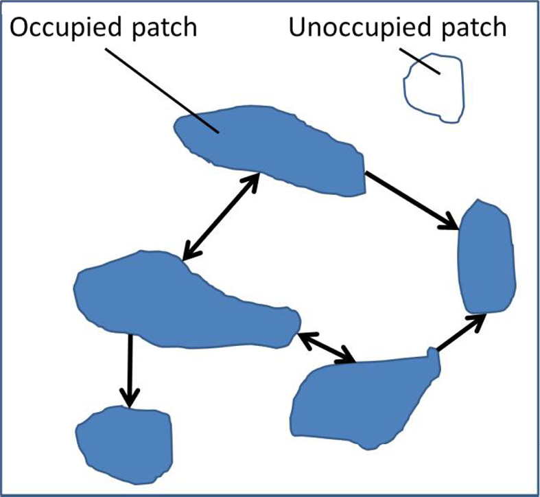
A metapopulation structure
In the source–sink model, most or all patches may be occupied (Figure 41). The population of interest appears to be widespread and may be abundant.
Figure 41.
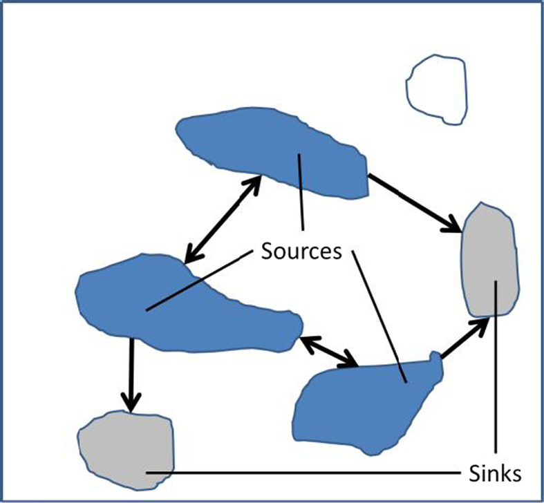
A source‐sink population structure
‘Sink’ populations (PGR < 1) occupying low‐quality patches; however, are maintained only by migration from ‘source’ populations (where PGR > 1).
Reduction of PGR in source populations can be disastrous and lead to rapid population collapse. This could be a result of use of a PPP in high‐quality patches. Sink populations are no longer topped up from source populations and will become extinct.
An example of an apparently successful and widespread species that once collapsed as a result of PPP (organochlorine) use is the sparrowhawk in England. Although it is once again widespread and breeding in woodlands across eastern England, many of these woodlands are sinks where PGR < 1 (Newton, 1998).
The real world is more complex than either Figures 39, 40 or 42. There are various landscape features such as rivers, hedgerows, and a variety of crops, that may act as either barriers or corridors between populations. In addition, populations will often not occur in neat patches but be more generally distributed. For these situations, landscape simulation is necessary. This may include both detailed representation of spatial structure, but can also include dynamic modelling of the spatial distribution of habitat quality, environmental conditions and mortality. These approaches are typically associated with detailed population structuring (see below) since fine population structure is needed to take advantage of this spatial heterogeneity.
Figure 42.
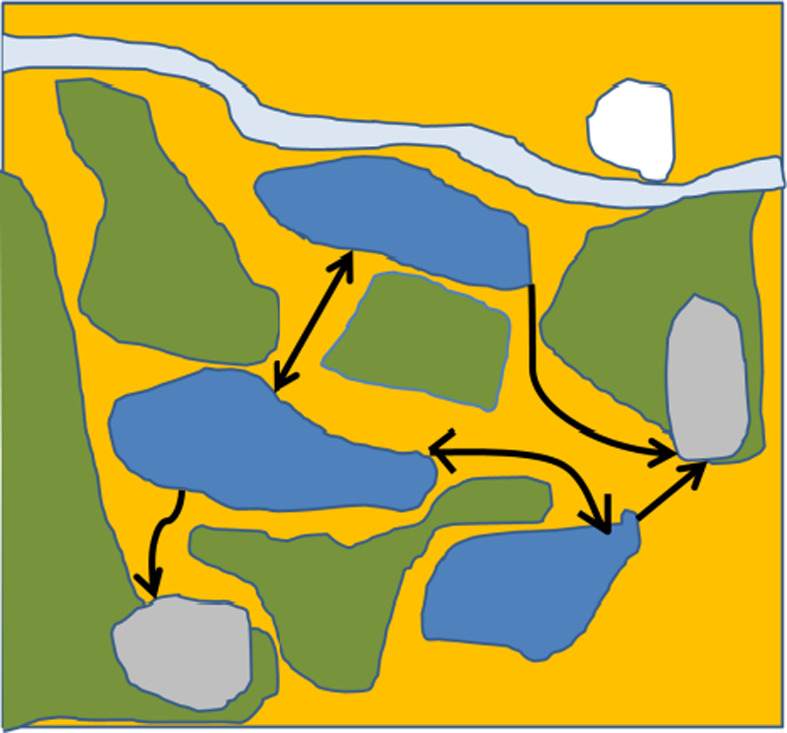
A landscape representation
Population structuring – theoretical considerations
Similar to spatial structure, a population can be considered as a single entity or split into smaller units, which in the extreme can be a detailed representation of individuals and their differences.
Like the spatial structuring, this population‐structuring axis is a continuum. At one extreme, we have the single entity exemplified by the two‐stage model presented above. This population can then be divided into smaller units, for example, in a stage structured model. Here, we can consider different life stages, e.g. eggs, larvae, adult and as well as reproduction, the rates of survival from one stage to the next. This allows for incorporation of stage‐specific information. This approach can be extended to spatially distributed populations but models become mathematically complex as more stages and processes are included. At some point as more structure is included, an individual‐based approach can be chosen. This is usually a pragmatic choice to overcome complexity in the system being modelled (Grimm, 1999). The theoretical advantage of this choice is primarily to incorporate feedback mechanisms between heterogeneous individuals and their environment. These individual representations can become highly detailed, including individual differences, e.g. in behaviour and genetics. For example, philopatry in amphibians may be important in their spatial dynamics, but requires detailed differences in behaviour of individuals.
Annex B – Relevant characteristics of ponds hosting amphibians to be able to estimate exposure
1.
Introduction
A pond is defined as a body of standing water 0.0010–2 ha in area, which usually holds water for at least 4 months of the year. We are interested in the distribution of ponds across the current EU.
This implies:
# ‘standing water’: slowly moving is still OK (order of few 1,000 m/day), but not fast flowing streams or rivers.
# ‘to 2 ha’: the water body should be delimited in size and especially length (so not be a stream). Sticking to the definition of up to 2 ha and assuming a minimum width of 30 m, the maximum length could be 667 m.
Our aim is to simulate environmental concentrations of pesticides in ponds for risk assessment for amphibians. The concentrations may be predicted as a function of time with the aid of a simple model and some additional assumptions. We would like to obtain a spatio‐temporal statistical distribution of environmental concentrations from which we could select the pond with the wished percentile worst‐casedness in concentration. We would like to be able to perform a ranking of the ponds across: (i) the entire EU, (ii) the individual EU Member States (including the UK), (iii) regions of ‘similar’ agro‐environmental–ecological conditions.
As we are interested in concentrations the water depth is an important characteristic we need (next to surface area of pond). As the aim is to use the data for pesticide registration a first criterion for selection of ponds is: they are located in an agricultural area (agriculture within 50 m of pond)
Required characteristics + explanation
The following attributes for the ponds are important:
(N.B. The bold items are most important)
-
1
surface area + time of observation (at least month, year)
-
2
water depth + time of observation (at least month, year)
-
3
drawdown
-
4
seasonality: truly seasonal, permanent or semi‐permanent
-
5
presence of inflow, or outflow, or both
-
6
soil type in which pond is located
-
7
land use in surrounding, (e.g. % arable in 0–5 m and 0–100 m perimeter around pond)
-
8
distance agricultural field ‐ edge of water
-
9
presence of vegetation on the edge of the pond
-
10
presence of amphibians?
If possible also:
-
11
presence of water plants inside pond, percentage surface area covered by plants
-
12
likely to contain water in spring or not, for at least one month ?
Concerning the location of the pond:
-
13
coordinates plus + EU‐Member State name.
Ad 1. Surface area + time of observation:
Lower limit: What is the smallest pond size that can be detected? Our proposal for upper limit: 2 ha.
Surface area of the ponds should be listed or be classified according to surface area in the following size classes: < 10 m2, 10–25 m2, 25–100 m2, 100–400 m2, 400–1,000 m2, 1,000–2,000 m2, 2,000–1 ha, 1–2 ha)
N.B. Small ponds (up to ~ 1,000 m2) are an important habitat for amphibians, so it is crucial that these ponds are included in the analysis.
Considering time of observation: for how many years the data are available? For reasons of simplicity a proposal could be to select an ‘average’ meteorological year, resulting in ‘average’ surface and water depth to be used. Maybe combined with surface area and water depth for the ‘last‐but‐one driest’ and ‘last‐but‐one wettest year’?
Ad 2. Water depth + time of observation:
An explanation should be added how the water depth has been calculated. What is its level of detail, which differences in depth have been captured? Was the water depth obtained by a calculation method (has this been validated?) or are measured depths used? Please state what the water level represents exactly: the average water depth over the entire pond, or the maximum water depth over the area of the pond?
Ad 3. Draw down:
The drawdown is a measure of how far water levels drop in summer compared to their bank‐full winter standing water levels
Ad 4. Seasonality:
We use the following definitions for seasonality:
Permanent: pond does not dry out
Semi‐permanent: pond dries out in drought years
Truly seasonal; pond dries out every year
Ad 5. Presence of inflow, outflow or both:
Is there a visible inflow or outflow of water into/out of the pond or both ?
Ad 6. Soil type:
Please describe also the used soil type classification system
Ad 7. Land use in surrounding:
As precise as possible, preferably crop type. Crucial for pesticide registration.
Ad 8. Distance agricultural field‐edge of water:
The distance between the nearest agricultural field and the edge‐of‐water is an important factor defining the spray‐drift deposition. Spray‐drift experts need the distance between the last row of crops and the edge‐of‐water to be able to predict the deposition.
Ad 9. Presence of vegetation on edge of the pond:
This is also an important factor for the spray‐drift deposition.
Ad 10. Presence of amphibians:
Is it possible to know whether amphibians are present or might be present ? Overlay with map on presence of amphibians possible?
Ad 11. Macrophytes:
Please state whether floating or emerging water plants are visible in the pond and the percentage of the surface area they cover.
Ad 12. Water in spring or not?
During the spring, i.e. the breeding season of amphibians the ponds should have water for at least one month to be able to host amphibians from eggs to metamorphosis to their terrestrial life stage.
Ad 13. Within EU or certain MS:
Easy to allocate.
Annex C – Overview on exposure routes for amphibians and reptiles and available exposure models
1.
Table 44 provides an overview on exposure routs for different amphibian and reptile terrestrial life stages.
Table 44.
Exposure routes – amphibians and reptiles terrestrial phase (other than ingestion)
| Medium | Available model | Unit | Description of ecotoxicological exposure quantity | |
|---|---|---|---|---|
| A‐Juvenile, adults | Soil | Dermal exposure residents | mg/m2 | Mass of ai dissolved per mass of soil |
| A‐Juvenile, adults | Plant | Time to re‐entry | mg/day | Only for dried residues |
| A‐Juvenile, adults | Air | Bystanders, residents, TIM | mg/m3 | Spray drift |
| R‐Eggs, juveniles, adults | Soil | PECsoil | mg/kg | Mass of ai dissolved per mass of soil |
| R‐Juveniles, adults | Plant, stone walls | Worker exposure (dermal), TIM | mg/m2 | Dislodgeable foliar residues |
| R‐Juvenile, adults | Air | Resident, bystander, TIM | mg/m3 | Spray drift |
| R‐Juvenile, adults | Air | Overspray + crop interception | mg/m2 | Direct overspray |
Annex D – Overview on existing risk assessment for birds and mammals
1.
1.1.
1.1.1.
Risk assessment for oral uptake:
The TER values are calculated for generic focal species in the first‐tier assessments according to the following formula:
TER = toxicity endpoint/DDD (daily dietary dose)
DDD = SV × application rate
SV = shortcut value = FIR/bw × RUD
FIR = daily food intake rate
bw = body weight
RUD = residue per unit dose (residues for different food items, e.g. insects, plants, seeds), mean RUD values are used for the reproductive risk assessment and 90%tile RUD values are used for acute risk assessment.
The RUD values are generic residue values per kg a.s. applied per ha, the unit is mg a.s./kg food item.
Conservative assumptions in the first‐tier risk assessment for birds and mammals:
In the first‐tier risk assessment, it is assumed that a bird obtains 100% of its food from the treated field.
Secondary poisoning:
For active substances with a log Pow > 3, an assessment of the risk posed by bioconcentration of the substance in the prey of birds and mammals shall be provided.
The risk assessment of secondary poisoning of earthworm eating birds and mammals is described in the EFSA birds and mammals GD (EFSA 2015a) on p. 71–73.
The bioconcentration factor (BCF) for earthworms is calculated and based on the BCF the concentration in earthworms is calculated.
The daily dietary dose (DDD) is calculated by multiplying the concentration in earthworms by 1.28 for mammals (10 g mammal eating 12.8 g worms per day) and by 1.05 for birds (100 g bird eating 104.6 g worms per day)
The TER is calculated with the long‐term NOAEL (TER = NOAEL/DDD). The trigger value is 5.
The risk assessment of secondary poisoning of fish eating birds and mammals is presented in the EFSA birds and mammals GD on p. 74.
The BCF for fish is available from the studies in the dossier and can be used to calculate the concentration in fish.
The daily dietary dose (DDD) is calculated by multiplication of the concentration in fish by 0.142 for mammals and by 0.159 for birds.
The TER is calculated with the long‐term NOAEL (TER = NOAEL/DDD). The trigger value is 5.
Conservative assumptions in the risk assessment of secondary poisoning for birds and mammals:
Only one food item is considered. One hundred per cent of the food is contaminated with the compound. The concentrations in earthworms are based on the full application rate and related soil or pore water concentrations in soil. For the concentrations in fish, the regulatory acceptable concentration is used (maximum concentration in surface water for which the risk to water organisms is considered to meet the protection goals).
Overall, it is assumed that the risk to amphibians and reptiles is covered by the assessment of the risk to birds and mammals for the food items earthworms and fish – this needs checking – look at the uptake rates for earthworm/fish eating amphibians and reptiles. Exposure via other prey items such as insects, amphibians and small mammals should be considered. Direct overspray of insects could be considered as a first‐tier approach and a worst‐case scenario for amphibians and reptiles.
Assessment of biomagnification in terrestrial food chains (p. 75 EFSA birds and mammals GD):
If information form, the toxicology section (absorption, distribution, metabolism and excretion (ADME) studies) indicates low potential of bioaccumulation then this assessment is not required.
Bioaccumulation factor (BAF) should be less than 1. It is calculated according to the following formula:
BAF = α × FIR/k2
α = fraction from ingested dose that is absorbed
k2 = rate constant for depuration, k2 = ln(2) × T1/2 (T = elimination half‐life)
FIR = food intake rate relative to body weight
Uptake of contaminated water by drinking:
Two scenarios are assessed:
Daily drinking water demand is satisfied from drinking from puddles in leaf axils (= leave scenario) (concentration of spray solution/5) or
drinking from puddles in the field (= puddle scenario) on the bare soil.
The drinking water uptake is calculated for a small granivorous bird (bw = 15.3 g, daily water uptake of 0.46 L/kg bw per day) and a small granivorous mammal (bw = 21.7 g, daily water uptake of 0.24 L/kg bw per day)
For the leaf axil scenario, only an acute risk assessment is conducted while for the puddle scenario also a long‐term risk assessment is conducted.
Conservative assumptions in the first‐tier risk assessment for birds and mammals:
In the first‐tier risk assessment, it is assumed that a bird obtains 100% of its drinking water from the treated field.
Risk assessment for granular formulations (EFSA birds and mammals GD p. 43–54):
This is only added for completeness to see which exposure routes are assessed for birds and mammals.
The following oral exposure routes are listed for evaluation:
Ingestion of granules as food.
Birds may ingest granules as grit.
Birds may mistake granules for small seed.
Birds and mammals may consume food contaminated with residues resulting from granular applications.
Birds and mammals may ingest granules when they eat food contaminated with soil.
Annex E – Endpoints available in dossiers from standard birds and mammal studies
1.
Birds:
For all avian and mammalian feeding studies, average achieved dose shall be reported, including where possible the dose in mg substance/kg body weight. The following endpoints are available in the dossiers as standard requirements.
Acute oral toxicity
Guidelines: OECD 223 or US EPA OCSPP 850.2100
Exposure: oral, single dose via gavage
Observation period: 14 days
Effects: mortality, LD50, the lethal threshold dose, time courses of response and recovery, the LD10 and LD20 shall be reported together with the no observed effect level (NOEL) and gross pathological findings.
Short‐term dietary toxicity: This test is only required if there is an indication from the mode of action or from the mammalian studies that the short‐term dietary test could result in a lower LD50 than the acute short‐term test.
Guidelines: OECD 205, US EPA OCSPP 850.2200
Exposure: oral over 5 days, ad libitum food uptake
Observation period: at least for 9 days
Effects: mortality, LD50, lowest lethal concentration (LLC), where possible, NOEC values, time courses of response and recovery and pathological findings shall be reported in such study.
Reproductive toxicity
Guidelines: OECD 206, US EPA OCSPP 850.2300
Exposure: oral, exposure of adults 10 weeks before egg laying and 8–10 weeks during egg laying, food uptake ad libitum, eggs are removed and artificially incubated, chicks are not exposed
Observation period: from 10 weeks before egg laying and at least 8 weeks during egg laying.
Effects: EC10, EC20 and NOEC in mg a.s./kg bw per day for the following:
Adult body weight and food consumption
Number of eggs laid per hen
The mean eggshell thickness
The proportion of eggs set
The proportion of fertile eggs with viable embryos
The proportion of eggs that hatch and produce chicks
The survival of chicks at 1 and 14 days of age.
Mammals:
For all avian and mammalian feeding studies, average achieved dose shall be reported, including where possible the dose in mg substance/kg body weight. The following endpoints are available in the dossiers as standard requirements.
Acute oral toxicity to mammals
Guidelines: OECD 420, OECD 423, OECD 425
Exposure: oral, single dose by gavage
Observation period: 14 days
Effects: mortality, LD50, unless otherwise needed, only female rats will be used, overall food consumption on the day of exposure as well as the time of onset and disappearance of overt clinical signs should be monitored.
Long term reproductive toxicity to mammals
Guidelines: OECD 416, the following tests may also be available: OECD 414, 407, 408
Exposure: oral, ad libitum via spiked food (the Guideline allows also gavage or exposure via drinking water) over the whole test duration starting with the first generation (during growth for at least one full spermatogenic cycle) and F1 until weaning of the F2 generation.
Observation period: from parental generation to weaning of F2
Effects:
The most sensitive and ecotoxicologically relevant mammalian long‐term toxicological endpoint (NOAEL) expressed as mg substance/kg bw per day shall be reported. Where EC10 and EC20 cannot be estimated an explanation shall be provided.
Typical observations/primary endpoints are: fertility, litter size and survival, growth, development and sexual maturation (of F1 generation).
In addition, there are developmental studies with rabbits and rats (such as OECD 414).
The EFSA birds and mammals GD considers the following endpoints as relevant for reproductive performance:
NOAEL for body weight change, behaviour effects and systemic toxicity
NOAEL for indices of gestation, litter size, pup and litter weight
NOAEL for indices of viability, pre‐ and post‐implantation loss
NOAEL for embryo/fetal toxicity including teratogenic effects
NOAEL for number abortions and number early delivery
NOAEL for systemic toxicity and effects on adult body weight
NOAEL for indices of post‐natal growth, indices of lactation and data on physical landmarks
NOAEL for survival and general toxicity up to sexual maturity
Annex F – Coverage of the risk to amphibians and reptiles by the human risk assessment
1.
Human exposure to plant protection products and the respective risk assessment is related to two main categories of exposure, the dietary and the non‐dietary exposure. The dietary exposure is relevant for the consumers of the agricultural products where pesticides can be present as residues on/in the different commodities. The non‐dietary exposure is relevant for the operators, workers, bystanders and residents of the rural areas.
For both dietary and non‐dietary risk assessment, the exposure levels, measured or estimated using mathematical models, are compared to the appropriate toxicological threshold values.
The toxicological threshold used for the dietary risk assessment is the acceptable daily intake (ADI). The basis for ADI setting is the chronic/long‐term toxicity studies, from which the highest dose that does not produce any adverse effects on the experimental animals is identified (WHO, 1987). The no observed adverse effect level (NOAEL) is divided by the appropriate assessment factor (usually 100) for extrapolation from animals to humans taking into consideration toxicokinetic and toxicodynamic variability as well as the human variability. In addition, for compounds that may produce adverse effects following subacute/acute exposure the acute reference dose (ARfD) is also established from the respective study(ies) with the application of the assessment factor (European Commission, 2011). Both the ADI and ARfD are considered to be ‘external’ doses since they do not reflect the absorbed amount of the substance through the gastrointestinal tract but the highest amount that can be ingested without any adverse effect on human health.
The toxicological threshold used for the non‐dietary risk assessment is the acceptable operator exposure level (AOEL). The basis for the AOEL are the repeated dose toxicity studies considering the most relevant toxicological endpoint in the most sensitive species. From these studies, the highest dose that does not produce any adverse effects on the experimental animals is identified. The NOAEL is then divided by the appropriate assessment factor (usually 100) for extrapolation from animals to humans as with other reference values. Usually, the studies that are used for the AOEL setting are oral exposure studies. For substances that may produce detrimental effects after a single day of exposure the acute acceptable operator exposure level (AAOEL) is to be established. Considering the new EFSA Guidance on the assessment of exposure of operators, workers, residents and bystanders in risk assessment for plant protection products, as noted by the European Commission (SANTE‐10832‐2015, 29 May 2015), the AAOEL is required for risk assessment. However, there is still no guidance for the derivation of the AAOEL. For the estimation of the AOELsystemic, the oral AOEL is corrected by the oral absorption factor when the extent of oral absorption is lower than 80% of the ingested amount, as identified in relevant ADME studies.
The units for both the ADI and AOEL values are mg/kg bw per day, whereas for ARfD it is mg/kg bw.
As far as it relates to dietary exposure, consumer exposure estimations (based on maximum residue levels in/on the different commodities and food consumption factor), toxicological thresholds (ADI and ARfD) and risk assessment, are not considered to provide any useful information either for exposure estimations or risk assessment for amphibians and reptiles. The non‐dietary human risk assessment, as a whole, is not applicable to A&R risk assessment, since the exposure scenarios and the hazard thresholds are specific to humans.
Annex G – Overview of important exposure routes, life stages and endpoints that need to be considered in the risk assessment for amphibians and reptiles
1.
The Tables 45 and 46 provide an overview on existing tests that cover the specific exposure routes/life stages/endpoints and on tests that could be developed to address exposure routes/life stages/endpoints not currently covered by standardised tests.
Table 45.
Overview of suitable test designs to address the different routes of exposure for all life stages and relevant endpoints in amphibians. Endpoints written in bold indicate that they are considered most relevant for the specific protection goals (SPGs) and should be addressed in the risk assessment. This judgement has its limitations and is based on expert judgement and the limited data currently available. The idea of the table is to illustrate which standard tests can be used to address the relevant combinations of exposure route/life stage/endpoints, and to show the current gaps in the standard test designs. X: Test with matching taxonomic group that is designed to cover the endpoint, life stage and exposure route, +: Test with matching taxonomic group that could be expanded to cover the endpoint, life stage and exposure route, o: Test that could be used for extrapolation of data between taxonomic groups or within the chosen taxon to cover the endpoint, life stage and exposure route
| Medium | Exposure route | Life stages exposed in the medium by the exposure route | Endpointsb | Tests | |||||
|---|---|---|---|---|---|---|---|---|---|
| Acute fish OECD 203 | Aquatic life cycle/reproductive testa | LAGDA | AMA | Overspray testa | Sediment testc | ||||
| Water | Contact/dermal | Egg/embryo | Mortality | + | Xd | ||||
| Malformation | + | Xd | |||||||
| Duration of development | + | Xd | |||||||
| Hatchling | Mortality | X | X | ||||||
| Growth | |||||||||
| Malformation | X | X | |||||||
| Duration of development | X | X | |||||||
| Behaviour | X | ||||||||
| Larvae/tadpole | Mortality | o | X | X | X | ||||
| Growth | X | X | X | ||||||
| Malformation | X | X | X | ||||||
| Duration of development | X | X | X | ||||||
| Behaviour | + | ||||||||
| Metamorphs | Duration of development | X | + | ||||||
| Success rate | X | + | |||||||
| Mortality | X | + | |||||||
| Growth | + | + | |||||||
| Sex ratio | X | + | |||||||
| Juvenile | Mortality | o | X | X | |||||
| Growth | X | X | |||||||
| Sex ratio | X | X | |||||||
| Behaviour | + | ||||||||
| Lesions | X | X | |||||||
| Adult | Mortality | o | |||||||
| Reproduction | X | ||||||||
| Behaviour | X/+e | ||||||||
| Lesions | X | ||||||||
| Oral | Juvenile | Mortality | + | + | |||||
| Growth | + | ||||||||
| Behaviour | |||||||||
| Sex ratio | |||||||||
| Lesions | |||||||||
| Adult | Mortality | + | + | ||||||
| Reproduction | + | ||||||||
| Behaviour | + | ||||||||
| Lesions | + | ||||||||
| Sediment | Contact/dermal | Hatchling | Mortality | o | |||||
| Growth | |||||||||
| Malformation | |||||||||
| Duration of development | |||||||||
| Behaviour | |||||||||
| Larvae/tadpole | Mortality | X | |||||||
| Growth | X | ||||||||
| Malformation | X | ||||||||
| Duration of development | |||||||||
| Behaviour | X | ||||||||
| Metamorphs | Duration of development | ||||||||
| Success rate | |||||||||
| Juvenile | Mortality | o | |||||||
| Growth | |||||||||
| Sex ratio | |||||||||
| Behaviour | |||||||||
| Lesions | |||||||||
| Adult | Mortality | o | |||||||
| Reproduction | |||||||||
| Behaviour | |||||||||
| Lesions | |||||||||
| Oral | Larvae/tadpole | Mortality | X | ||||||
| Growth | X | ||||||||
| Malformation | X | ||||||||
| Duration of development | |||||||||
| Behaviour | X | ||||||||
| Food | Oral | Larvae/tadpole | Mortality | + | |||||
| Growth | + | ||||||||
| Malformation | + | ||||||||
| Duration of development | + | ||||||||
| Behaviour | + | ||||||||
| Juvenile | Mortality | + | |||||||
| Growth | + | ||||||||
| Behaviour | + | ||||||||
| Sex ratio | |||||||||
| Lesions | |||||||||
| Adult | Mortality | ||||||||
| Reproduction | + | ||||||||
| Behaviour | + | ||||||||
| Lesions | |||||||||
| Overspray | Contact/dermal | Juvenile | Mortality | X | |||||
| Growth | X | ||||||||
| Behaviour | |||||||||
| Sex ratio | |||||||||
| Lesions | |||||||||
| Adult | Mortality | X | |||||||
| Reproduction | X | ||||||||
| Behaviour | |||||||||
| Lesions | |||||||||
| Soil | Contact/dermal | Juvenile | Mortality | + | |||||
| Growth | X | ||||||||
| Behaviour | |||||||||
| Sex ratio | |||||||||
| Lesions | |||||||||
| Adult | Mortality | + | |||||||
| Reproduction | X | ||||||||
| Behaviour | |||||||||
| Lesions | |||||||||
| Plants | Contact/dermal | Juvenile | Mortality | + | |||||
| Growth | X | ||||||||
| Behaviour | |||||||||
| Lesions | |||||||||
| Adult | Mortality | + | |||||||
| Reproduction | X | ||||||||
| Behaviour | |||||||||
| Lesions | |||||||||
| Water puddle | Contact/dermal | Juvenile | Mortality | o | |||||
| Growth | X | ||||||||
| Behaviour | |||||||||
| Sex ratio | |||||||||
| Lesions | |||||||||
| Adult | Mortality | o | |||||||
| Reproduction | X | ||||||||
| Behaviour | |||||||||
| Lesions | |||||||||
| Food (terrestrial) | Oral | Juvenile | Mortality | ||||||
| Growth | |||||||||
| Behaviour | |||||||||
| Sex ratio | |||||||||
| Lesions | |||||||||
| Adult | Mortality | ||||||||
| Reproduction | X | ||||||||
| Behaviour | |||||||||
| Lesions | |||||||||
OECD: Organization for Economic Co‐operation and Development; LAGDA: Larval Amphibian Growth and Development Assay; AMA: Amphibian Metamorphosis Assay.
Standardised test does not exist but could be developed.
Endpoints reflecting effects which can be measured in the life stage.
ASTM E2591‐07 (2013) or OPPTS 850.1800.
The exposure route is not exactly comparable because in LAGDA the jelly layer surrounding the embryo is removed.
Behavioural effects such as amplexus success rate, time until amplexus formation and duration of amplexus are routinely included in the test (Gyllenhammar et al., 2009; Berg, 2009), whereas behavioural effects such as male–male competitive mating and calling behaviour (Behrends et al., 2010; Hayes et al., 2010) could also be observed.
Table 46.
Overview of suitable test designs to address the different routes of exposure for all life stages and relevant endpoints in reptiles. Endpoints written in bold indicate that they are considered most relevant for the specific protection goals (SPGs) and should be addressed in the risk assessment. This judgement has its limitations and is based on expert judgement and the limited data currently available. The idea of the table is to illustrate which standard tests can be used to address the relevant combinations of exposure route/life stage/endpoints, and to show the current gaps in the standard test designs. X: Test with matching taxonomic group that is designed to cover the endpoint, life stage and exposure route, +: Test with matching taxonomic group that could be expanded to cover the endpoint, life stage and exposure route, o: Test that could be used for extrapolation of data between taxonomic groups or within the chosen taxon to cover the endpoint, life stage and exposure route
| Medium | Exposure route | Life stages | Endpointsb | Tests | ||||
|---|---|---|---|---|---|---|---|---|
| Avian Acute Oral (OECD 223) | Avian Reproductive Test (OECD 206) | In ovo toxicity test (test to be developed)a | Acute Overspray test (same test as for amphibians)a | Chronic toxicity test via dermal exposure on soila | ||||
| Soil | Contact/dermal | Egg/embryo | Mortality | X | ||||
| Time to hatch | X | |||||||
| Hatchling biometry | X | |||||||
| Sex ratio | X | |||||||
| Juvenile | Mortality | o | ||||||
| Growth | X | |||||||
| Behaviour | X | |||||||
| Lesions | X | |||||||
| Metabolic Rate | X | |||||||
| Adult | Mortality | o | ||||||
| Reproduction | X | |||||||
| Behaviour | X | |||||||
| Lesions | X | |||||||
| Metabolic Rate | X | |||||||
| Plants | Contact/dermal | Juvenile | Mortality | o | ||||
| Growth | o | |||||||
| Behaviour | o | |||||||
| Lesions | o | |||||||
| Metabolic Rate | o | |||||||
| Adult | Mortality | o | ||||||
| Reproduction | o | |||||||
| Behaviour | o | |||||||
| Lesions | o | |||||||
| Metabolic Rate | o | |||||||
| Overspray | Dermal | Juvenile | Mortality | o | ||||
| Behaviour | + | |||||||
| Lesions | + | |||||||
| Metabolic Rate | + | |||||||
| Adult | Mortality | o | ||||||
| Reproduction | ||||||||
| Behaviour | + | |||||||
| Lesions | + | |||||||
| Metabolic Rate | + | |||||||
| Food | Oral | Juvenile | Mortality | o | ||||
| Growth | ||||||||
| Behaviour | ||||||||
| Lesions | ||||||||
| Metabolic Rate | ||||||||
| Adult | Mortality | o | ||||||
| Reproduction | o | |||||||
| Behaviour | o | |||||||
| Lesions | o | |||||||
| Metabolic Rate | o | |||||||
Standardised test does not exist but could be developed.
Endpoints reflecting effects which can be observed in the life stage.
Appendix A – Species list
1.
Table 47 provides a list of amphibian and reptile species in the European Union (excluding overseas, Macaronesian and northern African territories), classified by assessment groups suggested for further identification of focal species (see Section 2.5 for details).
Table 47.
Overview on amphibian and reptile species in the European Union
| Assessment group | Family | Species | Distributed in zones | Present in arable land | ||
|---|---|---|---|---|---|---|
| South | Centre | North | ||||
| Caudates | Plethodontidae | Speleomantes ambrosii | X | |||
| Speleomantes flavus | X | |||||
| Speleomantes genei | X | |||||
| Speleomantes imperialis | X | |||||
| Speleomantes italicus | X | |||||
| Speleomantes sarrabusensis | X | |||||
| Speleomantes strinatii | X | |||||
| Speleomantes supramontis | X | |||||
| Proteidae | Proteus anguinus | X | ||||
| Salamandridae | Calotriton arnoldi | X | ||||
| Calotriton asper | X | |||||
| Chioglossa lusitanica | X | |||||
| Euproctus montanus | X | |||||
| Euproctus platycephalus | X | |||||
| Ichthyosaura alpestris | X | X | X | |||
| Lissotriton boscai | X | X | ||||
| Lissotriton helveticus | X | X | X | |||
| Lissotriton italicus | X | X | ||||
| Lissotriton montandoni | X | X | X | |||
| Lissotriton vulgaris | X | X | X | X | ||
| Lyciasalamandra helverseni | X | |||||
| Lyciasalamandra luschani | X | |||||
| Pleurodeles waltl | X | |||||
| Salamandra algira | X | |||||
| Salamandra atra | X | X | ||||
| Salamandra corsica | X | |||||
| Salamandra lanzai | X | |||||
| Salamandra salamandra | X | X | X | |||
| Salamandrina perspicillata | X | |||||
| Salamandrina terdigitata | X | |||||
| Triturus carnifex | X | X | ||||
| Triturus cristatus | X | X | X | X | ||
| Triturus dobrogicus | X | X | X | |||
| Triturus karelinii | X | X | ||||
| Triturus marmoratus | X | X | ||||
| Triturus pygmaeus | X | X | ||||
| Anurans | Alytidae | Alytes cisternasii | X | |||
| Alytes dickhilleni | X | |||||
| Alytes muletensis | X | |||||
| Alytes obstetricans | X | X | X | |||
| Discoglossus galganoi | X | X | ||||
| Discoglossus jeanneae | X | |||||
| Discoglossus montalentii | X | |||||
| Discoglossus pictus | X | X | ||||
| Discoglossus sardus | X | |||||
| Bombinatoridae | Bombina bombina | X | X | X | X | |
| Bombina variegata | X | X | X | |||
| Bombina pachypus | X | X | ||||
| Pelobatidae | Pelobates fuscus | X | X | X | X | |
| Pelobates cultripes | X | |||||
| Pelobates syriacus | X | X | X | |||
| Pelodytidae | Pelodytes ibericus | X | X | |||
| Pelodytes punctatus | X | |||||
| Hylidae | Hyla arborea | X | X | X | X | |
| Hyla intermedia | X | X | ||||
| Hyla meridionalis | X | |||||
| Hyla sarda | X | |||||
| Hyla savignyi | X | X | ||||
| Bufonidae | Bufo bufo | X | X | X | X | |
| Bufotes balearicus | X | X | ||||
| Bufotes boulengeri | X | X | ||||
| Bufotes siculus | X | X | ||||
| Bufotes variabilis | X | X | X | |||
| Bufotes viridis | X | X | X | X | ||
| Epidalea calamita | X | X | X | X | ||
| Ranidae | Pelophylax bedriagae | X | X | |||
| Pelophylax bergeri | X | |||||
| Pelophylax cerigensis | X | X | ||||
| Pelophylax cretensis | X | |||||
| Pelophylax epeiroticus | X | |||||
| Pelophylax esculentus | X | X | X | X | ||
| Pelophylax hispanicus | X | |||||
| Pelophylax kurtmuelleri | X | |||||
| Pelophylax lessonae | X | X | X | X | ||
| Pelophylax perezi | X | X | ||||
| Pelophylax ridibundus | X | X | X | X | ||
| Rana arvalis | X | X | X | X | ||
| Rana dalmatina | X | X | ||||
| Rana graeca | X | |||||
| Rana iberica | X | |||||
| Rana italica | X | |||||
| Rana latastei | X | |||||
| Rana pyrenaica | X | |||||
| Rana temporaria | X | X | X | X | ||
| Tortoises | Testudinidae | Testudo graeca | X | X | ||
| Testudo hermanni | X | X | ||||
| Testudo marginata | X | |||||
| Terrapins | Emydidae | Emys orbicularis | X | X | X | |
| Emys trinacris | X | |||||
| Geoemydidae | Mauremys leprosa | X | ||||
| Mauremys rivulata | X | |||||
| Saurians | Agamidae | Stellagama stellio | X | X | ||
| Anguidae | Anguis cephalonnica | X | X | |||
| Anguis fragilis | X | X | X | |||
| Pseudopus apodus | X | |||||
| Chamaeleonidae | Chamaeleo chamaeleon | X | ||||
| Gekkonidae | Hemidactylus turcicus | X | ||||
| Mediodactylus kotschyi | X | X | ||||
| Lacertidae | Acanthodactylus erythrurus | X | X | |||
| Acanthodactylus schreiberi | X | |||||
| Algyroides fitzingeri | X | X | ||||
| Algyroides marchi | X | |||||
| Algyroides moreoticus | X | |||||
| Algyroides nigropunctatus | X | X | ||||
| Anatololacerta anatolica | X | |||||
| Anatololacerta oertzeni | X | |||||
| Archaeolacerta bedriagae | X | |||||
| Dalmatolacerta oxycephala | X | |||||
| Darevskia praticola | X | X | ||||
| Dinarolacerta mosorensis | X | |||||
| Eremias arguta | X | |||||
| Hellenolacerta graeca | X | |||||
| Iberolacerta aranica | X | |||||
| Iberolacerta aurelioi | X | |||||
| Iberolacerta bonnali | X | |||||
| Iberolacerta cyreni | X | |||||
| Iberolacerta galani | X | |||||
| Iberolacerta horvathi | X | X | ||||
| Iberolacerta martinezricai | X | |||||
| Iberolacerta monticola | X | |||||
| Lacerta agilis | X | X | X | X | ||
| Lacerta bilineata | X | X | X | |||
| Lacerta schreiberi | X | |||||
| Lacerta trilineata | X | X | X | |||
| Lacerta viridis | X | X | X | |||
| Ophisops elegans | X | |||||
| Phoenicolacerta troodica | X | |||||
| Podarcis bocagei | X | |||||
| Podarcis carbonelli | X | |||||
| Podarcis cretensis | X | |||||
| Podarcis erhardii | X | |||||
| Podarcis filfolensis | X | X | ||||
| Podarcis gaigeae | X | |||||
| Podarcis hispanicus | X | |||||
| Podarcis levendis | X | |||||
| Podarcis lilfordi | X | |||||
| Podarcis melisellensis | X | |||||
| Podarcis milensis | X | X | ||||
| Podarcis muralis | X | X | X | |||
| Podarcis peloponnesiacus | X | X | ||||
| Podarcis pityusensis | X | X | ||||
| Podarcis raffonei | X | |||||
| Podarcis siculus | X | X | ||||
| Podarcis tauricus | X | X | X | |||
| Podarcis tiliguerta | X | X | ||||
| Podarcis vaucheri | X | |||||
| Podarcis waglerianus | X | X | ||||
| Psammodromus algirus | X | X | ||||
| Psammodromus hispanicus | X | X | ||||
| Psammodromus jeanneae | X | |||||
| Psammodromus manuelae | X | |||||
| Timon lepidus | X | X | ||||
| Zootoca vivipara | X | X | X | |||
| Phyllodactylidae | Tarentola mauritanica | X | X | |||
| Scincidae | Ablepharus budaki | X | ||||
| Ablepharus kitaibelii | X | X | ||||
| Chalcides bedriagai | X | X | ||||
| Chalcides chalcides | X | |||||
| Chalcides ocellatus | X | |||||
| Chalcides striatus | X | X | ||||
| Ophiomorus punctatissimus | X | |||||
| Trachylepis aurata | X | X | ||||
| Trachylepis vittata | X | X | ||||
| Sphaerodactylidae | Euleptes europaea | X | ||||
| Saurodactylus mauritanicus | X | |||||
| Typhlopidae | Typhlops vermicularis | X | X | |||
| Blind snakes | Amphisbaenidae | Blanus cinereus | X | X | ||
| Blanus strauchi | X | X | ||||
| Fully terrestrial snakes | Colubridae | Coronella austriaca | X | X | X | |
| Coronella girondica | X | |||||
| Dolichophis caspius | X | X | ||||
| Dolichophis jugularis | X | X | ||||
| Eirenis modestus | X | X | ||||
| Elaphe quatuorlineata | X | X | ||||
| Elaphe sauromates | X | X | ||||
| Hemorhois nummifer | X | |||||
| Hemorrhois algirus | X | X | ||||
| Hemorrhois hippocrepis | X | X | ||||
| Hierophis cypriensis | X | |||||
| Hierophis gemonensis | X | |||||
| Hierophis viridiflavus | X | X | ||||
| Macroprotodon brevis | X | |||||
| Macroprotodon cucullatus | X | X | ||||
| Platyceps collaris | X | X | ||||
| Platyceps najadum | X | X | ||||
| Rhinechis scalaris | X | X | ||||
| Telescopus fallax | X | X | ||||
| Zamenis lineatus | X | X | ||||
| Zamenis longissimus | X | X | X | |||
| Zamenis situla | X | |||||
| Erycidae | Eryx jaculus | X | X | |||
| Psammophidae | Malpolon monspessulanus | X | X | |||
| Malpolon insignitus | X | |||||
| Viperidae | Vipera ammodytes | X | X | X | ||
| Vipera berus | X | X | X | X | ||
| Vipera aspis | X | X | X | |||
| Montivipera xanthina | X | X | ||||
| Vipera seoanei | X | X | ||||
| Vipera latastei | X | |||||
| Vipera ursinii | X | X | ||||
| Macrovipera schweizeri | X | X | ||||
| Water snakes | Natricidae | Natrix natrix | X | X | X | X |
| Natrix tessellata | X | X | ||||
| Natrix maura | X | X | X | |||
Appendix B – Consequences of choices made by risk managers concerning the effects of intended PPP use on amphibians and reptiles
1.
Table 48 provides an overview on the consequences of different choices for the level of protection.
Table 48.
Overview on the consequences of the different protection goals options
| Amphibians and reptiles as key drivers of | Consequences of option choice regarding the effects of intended PPP use on amphibians and reptiles | ||
|---|---|---|---|
| Option: below the limit of operation | Option: Limit of operation | If above limit of operation | |
|
Provisioning services: Biodiversity Genetic resources Cultural services Food and pharmaceutical resources |
|
|
|
|
Continued: Biodiversity Genetic resources Cultural services Food and pharmaceutical resources |
|
|
|
|
Supporting services as Nutrient cycling Soil structure formation Food‐web support |
|
|
|
|
Regulating services as Pest and pathogen control Invasion resistance |
|
|
|
European Union: Regulation (EC) No 1107/2009 of the European Parliament and of the Council concerning the placing of plant protection products on the market and repealing Council Directives 79/117/EEC and 91/414/EEC. 21 October 2009. Official Journal of the European Union L 309, 24 November 2009, 50 pp.
Council Directive 92/43/EEC of 21 May 1992 on the conservation of natural habitats and of wild fauna and flora.
2009/2108(INI) Report on the implementation of EU legislation aiming at the conservation of biodiversity.
2011/244(INI) Communication: on our life insurance, our natural capital: an EU biodiversity strategy to 2020 Committee on the Environment, Public Health and Food Safety.
United Nations General Assembly (2015): Resolution adopted by the General Assembly on 25 September 2015. Transforming our world: the 2030 Agenda for Sustainable Development. Distr. General, 21 October 2015. Seventieth session, Agenda items 15 and 116, A/RES/70/1, 35 pp.
COM/2006/0232 final (2006): Proposal for a Directive of the European Parliament and of the Council establishing a framework for the protection of soil and amending Directive 2004/35/EC.
Council Directive 79/409/EEC of 2 April 1979 on the conservation of wild birds.
Directive 2009/128/EC of the European Parliament and of the Council of 21 October 2009 establishing a framework for Community action to achieve the sustainable use of pesticides.
Appendix C – Dimensions and surrounding land use of ponds in Spain, United Kingdom and Switzerland and comparison with FOCUS water bodies
1.
The working group gathered some data on the presence and size of ponds in a number of Member States. The databases for Spain and the Aargau canton in Switzerland contain only water bodies in which amphibians have been observed, while the database for the UK is much larger. Below, we present an analysis of the information contained in these databases with respect to (i) water surface area, water depth and water volume, and (ii) surrounding land use. The aim of this analysis was to establish sizes of ponds (and other water bodies) that serve or may serve as aquatic habitat for amphibians and in addition, establish whether ponds (or other water bodies) that serve as aquatic habitats for amphibians, are associated to agricultural land use in their surroundings. In this way, we are able to evaluate whether the amphibians are likely to be exposed to pesticides residues in their aquatic habitat.
A second aim was to compare the amphibian ponds to the so‐called FOCUS surface water bodies that are currently used in the risk assessment for the aquatic ecosystem at EU level: a pond, ditch and stream. The FOCUS pond measures 30 × 30 m and has a water depth of approximately 1 m and a surrounding, pesticide‐treated area of 4,500 m2 contributes its runoff or drainage water to the pond. The FOCUS ditch and stream are 100 m long, 1 m wide (rectangular cross‐section) and a 1 ha‐treated agricultural field delivers its runoff or drainage to the ditch or stream. Upstream of the ditch two ha of untreated agricultural fields deliver drainage flows, while the stream is fed by a 100‐ha upstream catchment of which 20 ha are treated with pesticides. The three water bodies receive spray‐drift deposition at the moment pesticides are applied on the adjacent field.
Spain
The database of the Spanish ponds was built with the data of the program SARE (monitoring of Spanish amphibians and reptiles) developed by the Spanish Herpetological Society. Details on the program can be found at http://siare.herpetologica.es/sare (available in Spanish only). The Spanish Herpetological Society kindly provided the entire database of ponds.
The SARE monitoring is carried out by volunteers who select one or several cells of the 10 × 10 km UTM grid. Within each cell, the person responsible for the monitoring must design the sampling, as part of which at least three water points have to be selected for sampling aquatic amphibians. When designing the monitoring, the volunteers record some information about the water points, including dimensions like the surface area (for ponds, for which surface shape is assumed to be elliptical, lengths of the major and minor axes are collected) and maximum depth of the water column, and characteristics of the surrounding habitat. Once the sampling strategy has been designed, the volunteer sends it to a regional coordinator who validates it. Then, the full sampling of each cell (including all water points and transects in terrestrial habitats in between) is repeated several times per year and the number of observed specimens is recorded. Since the objective of the program is to have long‐term trends in amphibian and reptile populations at the national level, it is expected that volunteers repeat the process year after year as long as they can. With this purpose, the program coordinators encourage volunteers to select cells that are easily reachable (i.e. located close to where they live, work or spend time regularly). It may happen that a volunteer must, at some point, redesign the sampling strategy because something has changed in the sampled habitat (e.g. a water body has desiccated). It also may happen that significant changes are observed in the characteristics of the water bodies, which means that the dimensions have to be recorded again for the same point. For this reason, the same pond may appear more than once in the database.
The first data of the program were recorded in 2010. More data are available for the first years of the program (2010 and 2011) because ponds are characterised when volunteers incorporate to the program, and this happened mostly during the initial years; afterwards, the number of volunteers contributing to the program dropped.
The database of ponds sampled as part of the SARE program provides a very good overview of amphibian breeding habitats. Contrarily to other pond inventories, these ponds are included here precisely because they constitute amphibian breeding habitats, and with such purpose have been selected by volunteer herpetologists (either amateur or professional) who have a good knowledge on the habitats they are sampling. It is true that a bias may exist in the election of ponds towards those harbouring a higher number of species, and this may exclude other amphibian breeding habitats that do not attract so many species. These under‐represented habitats can be, on the one hand, very permanent waters that, because of the frequent presence of fish, are not often used by most amphibians, and also that are difficult to sample because of their dimensions. On the other hand, shallow waters like puddles, that can also be used as breeding habitat by some species, are also under‐represented because of the difficulties that their unpredictability supposes for a continued monitoring over time.
Upon our request, the presence of arable land in the immediate surroundings of the amphibian ponds was assessed by the volunteers for 151 the 794 water bodies in the period September–November 2016. This was done to be able to evaluate whether the ponds were liable to be contaminated by the agricultural use of pesticides.
The SARE database contained 794 unique records for water bodies. The water bodies have been classified as ponds (421), artificial pool (152), dam/reservoir (66), lagoon/lake (21), river (30), stream (85) and wetland/marsh (19). Water depth, water surface area and water volume were analysed of all water bodies. First, the database was corrected, as some water depths (e.g. 100 m) were not plausible. In records of ponds, artificial pools, and streams in which the water depth was more than 10 m and the minor axis was less than or equal to 10 m, it was assumed that the depth was reported in cm instead of m, and the depth was converted to m. This was done for 23 ponds.
Water depth
For 10 water bodies, the depth was not reported. The frequency and cumulative frequency distribution of the remaining 784 water bodies is given in Figure 43 which shows that 18% of the water bodies has a water depth of 30 cm or less, i.e. the minimum water depth of the FOCUS ditches and streams. In total 70% of the water bodies is less than or equal to 1 m deep, i.e. the depth of the FOCUS pond.
Figure 43.
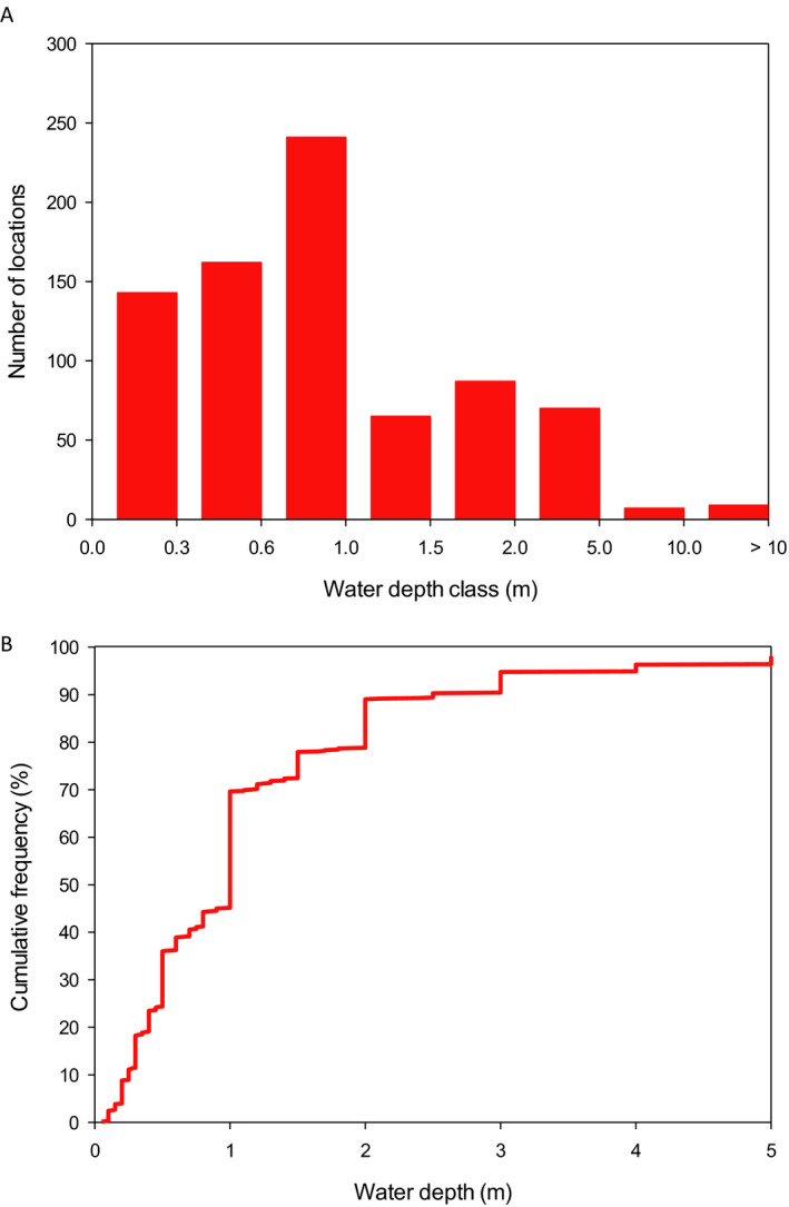
Frequency (A) and cumulative frequency (B) distribution of water depth of 784 water bodies in Spain. Note that in graph 1A the x‐axis is not linear and that all class boundaries are indicated. In graph 1B, water bodies with a depth greater than 5 m have not been included.
Water surface area
The water surface area of the 794 water bodies was calculated from the major and minor axis lengths according to the surface area of an ellipse: π × a × b (with a and b being the major and minor axis length). The frequency distributions are given for all 794 records. Figure 44 shows that 59% of the water bodies has a water surface area of less than or equal to 100 m2 (the surface area of the 100 m × 1 m FOCUS ditches and streams) and 87% an area of less than 900 m2 (the surface area of the 30 m × 30 m FOCUS ponds).
Figure 44.
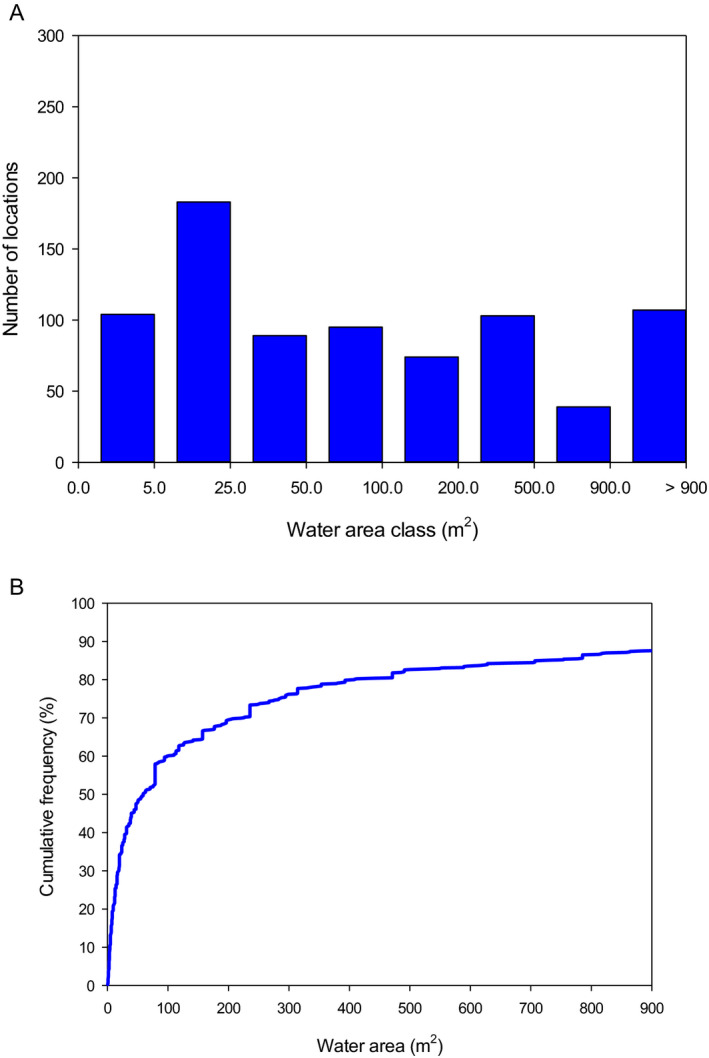
Frequency (A) and cumulative frequency distribution (B) of water surface area of 794 water bodies in Spain. Note that in graph A the x‐axis is not linear and that all class boundaries are indicated. In graph B, water bodies with an area greater than 900 m2 have not been included
Water volume
The water volume of the water bodies was calculated by volume = depth × area. As the recorded depth is the maximum depth in the ponds, the water volume will be somewhat overestimated. The frequency distributions are given for 784 records, for which a water depth was available. Figure 45 shows that 41% of the water bodies have a volume of less than 25 m3, 52% less than 50 m3 (the minimum water volume of FOCUS ditches and streams is 30 m3) and that 84% of the water bodies have a water volume of less than 900 m3 (the water volume of the FOCUS ponds).
Figure 45.
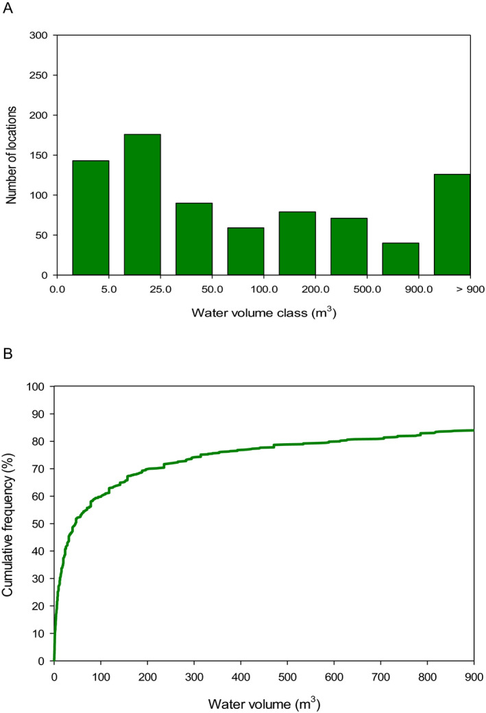
Frequency (A) and cumulative frequency distribution(B) of water volume of 784 water bodies in Spain. Note that in graph A the x‐axis is not linear and that all class boundaries are indicated. In graph B, water bodies with a volume greater than 900 m3 have not been included
Land use
The data on land use in the immediate surroundings (< 100 m) of 151 Spanish ponds indicate that for 81 of these of the ponds the surrounding land use is non‐agricultural. For the remaining 70 ponds, agricultural fields are nearby, for 32 ponds the distance edge‐of‐field to pond water is 0–10 m, for 21 ponds the distance is 10–20 m and for 17 ponds 20–100 m. Of the 70 ponds with agricultural fields nearby, 13 ponds are completely surrounded by the agricultural fields. Figure 46 presents the land use as function of the surface water area class of the ponds. It demonstrates that for all size classes arable and non‐arable land are approximately equally present, except for the ponds of less than 5 m2 area, which are predominantly surrounded by non‐arable land. So, these data demonstrate that a non‐negligible part of the Spanish ponds in which amphibians live, are likely to receive pesticides residues.
Figure 46.
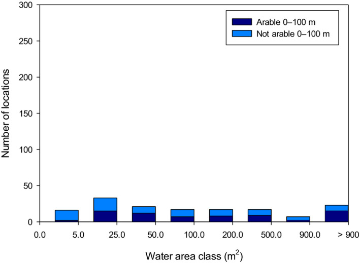
Frequency distribution of water surface area of the 70 ponds in Spain where a arable land use was observed in the 0–100 m distance zone from the perimeter of the pond, plus the remaining 81 ponds
Switzerland
The pond data from Switzerland stem from the amphibian monitoring programme in canton Aargau in the north of Switzerland which has been conducted since 2006 (Ref: Kanton Aargau, Abteilung Landschaft und Gewässer, Projekt Amphibienmonitoring Aargau, 2016). The purpose of the programme is to survey eight amphibian populations. Therefore, the selection of ponds is driven by the occurrence of one these eight species (tree frog, natterjack toad, midwife toad, yellow‐bellied toad, marsh frog, water frogs (all other types), great crested newt and common newt), which mainly occur in open areas. Ponds or streams in forests preferred by early breeding species such as common toad, common frog and fire salamander are poorly covered. The ponds are monitored three times per year by volunteers according to a standardised method. Next to counting the amphibian population, the surface area of the ponds (estimated size of all fragmented ponds in a pit combined), the water level (fluctuating, stable, unknown), exposure to sunlight and vegetation are estimated. Neither the depth nor the surrounding area is recorded. The data regarding the pond surface is estimated by volunteers during the period mid‐June to end of July (with exceptions between March and September).
Aargau can be described as a canton with intensive agriculture. Some of the monitored ponds were created by the farmers as ecological compensation in agricultural areas to obtain subsidies. For these two reasons, the data will include ponds close to fields (in Switzerland a buffer strip of at least 3 m to surface waters needs to be adhered to) and further afield.
The Swiss database on Aargau contained 754 unique records for water bodies. The water surface area was analysed. Water depth and water volume were not recorded.
Water surface area
For 25 water bodies, the water surface area was not recorded; hence, for 729 water bodies, the water surface area is plotted in frequency graphs in Figure 47. The figure shows that 52% of the water bodies has a surface area of less than or 100 m2 (the area of the FOCUS ditches and streams) and 89% an area of less than 900 m2 (the area of the FOCUS ponds).
Figure 47.
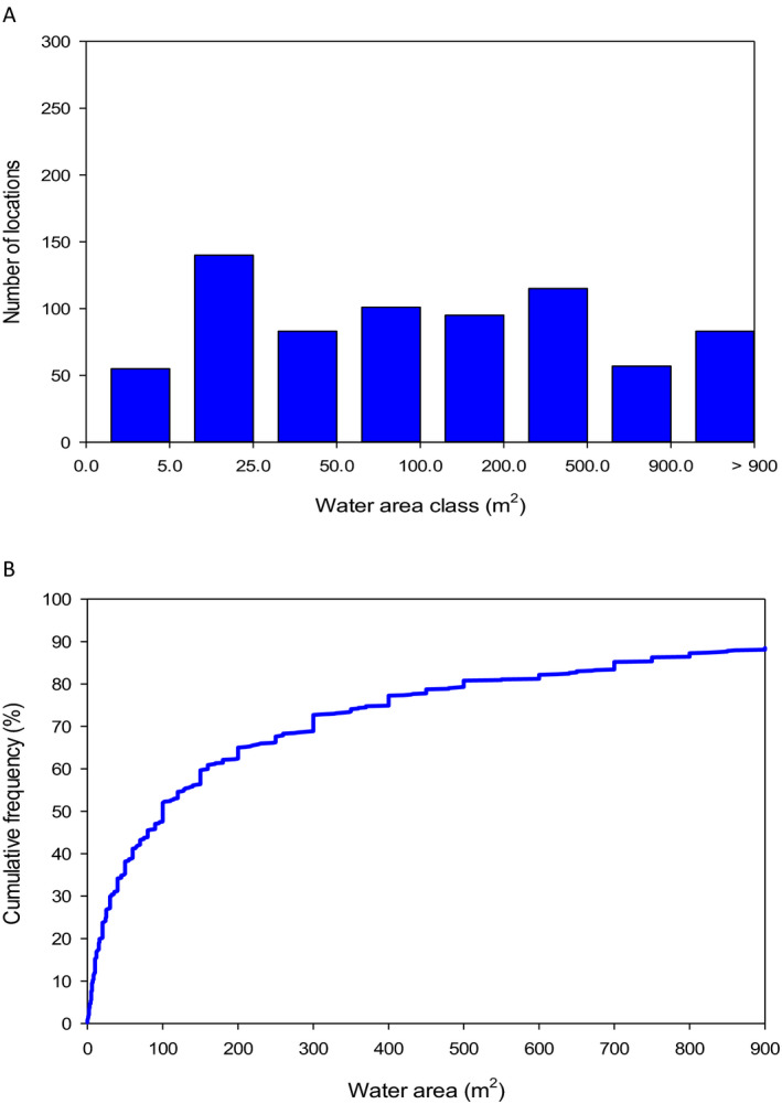
Frequency (A) and cumulative frequency distribution (B) of water surface area of 729 water bodies in canton Aargau, Switzerland. Note that in graph 4A the x‐axis is not linear and that all class boundaries are indicated. In graph 4B, water bodies with a volume greater than 900 m3 have not been included
Land use
There are no data for the Swiss canton Aargau ponds that specify the land use in their immediate surroundings. So, we are not able to evaluate on a quantitative basis whether the amphibians in these ponds are likely to be exposed to pesticides residues in their aquatic habitat. However, the Aargau canton being a canton with intensive agriculture and a good distribution of amphibian populations, a number of the ponds in the database are likely to represent amphibian habitats that may receive pesticide residues.
United Kingdom
In the United Kingdom, the current state of ponds was described by the Countryside Survey of 2007 (Williams et al., 2010). The survey covered a total of 591 1 × 1 km2 samples spread across England, Scotland and Wales. A pond was defined as a body of standing water of 25 m2 to 2 ha, in area, which usually holds water for at least 4 months of the year. So, in principle ponds smaller than 25 m2 were not recorded, while they might have been present. The survey made an inventory of pond number within the 1 × 1 km2 and of many properties of the ponds, such as biodiversity and ecological quality determined by e.g. plant species present, physical and chemical condition of ponds, such as nutrient status, hydrological properties, e.g. inflow and outflow, drawdown (= water level drop in summer compared to the bank‐full winter water level) and water surface area and adjacent land use. For example, the survey demonstrated that almost two‐thirds (63%) of ponds were directly linked to the stream network and that a third of these ponds had an inflow, but no outflow, suggesting that many ponds intercept and retain drainage water. In our analysis, we especially focussed on the water surface area, water depth, surrounding land use and presence of amphibians in the ponds.
The database from CountrySide Survey (2007) contains 259 records with ponds for which the water surface area has been measured (POND_WATER_QUALITY csv file). Water depth has been recorded, but only for a limited number of ponds as the time and equipment lacked to measure the maximum depth in ponds, where it was too deep to wade (pers. comm. J. Biggs, 11 Nov 2016).
Water depth
For 109 ponds, the depth had been measured. The frequency distribution of these 109 ponds is given in Figure 48 as a function of the mean water depth of the pond. The figure shows that 69 of the 109 ponds for which the water depth was measured have a water depth below 0.3 m. As the maximum depth was not measured in the remaining 150 ponds where it was too deep to wade, the data on water depth is clearly biased with maximum water depth over 1 m being not represented. So, in 27% (69/259) of the ponds, the water depth is smaller than 30 cm, and in 42% (109/259) the water depth is smaller than 1 m.
Figure 48.
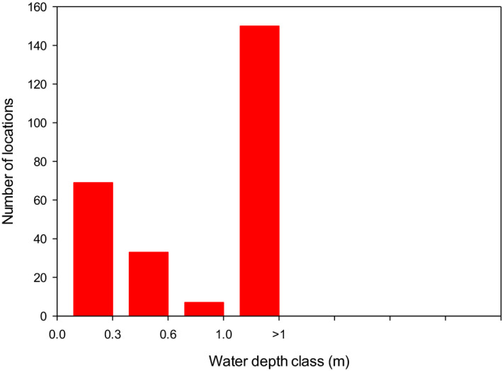
Frequency (A) distribution of water depth of 259 water bodies in the UK. For 150 ponds, the mean water depth was not measured because they were to deep to wade (indicated in the class with depth > 1 m). Note that the x‐axis is not linear and that all class boundaries are indicated
Water surface area
For two ponds, the surface area was not recorded, hence we plotted the areas for 257 ponds (Figure 49). The size of the surface areas has been estimated at the time of the survey, often in the period May–October 2007. In total, 23% of the ponds has a water surface area of less than or equal to 100 m2 (the surface area of FOCUS ditches and streams) and 79% an area of less than 900 m2 (the surface area of the FOCUS ponds). Small ponds with areas below 25 m2 were not included in the survey given the pond definition (required surface area of 25 m2 to 2 ha), although they are widely present in the UK landscape. This implies that the percentages given above represent an underestimation compared to reality.
Figure 49.
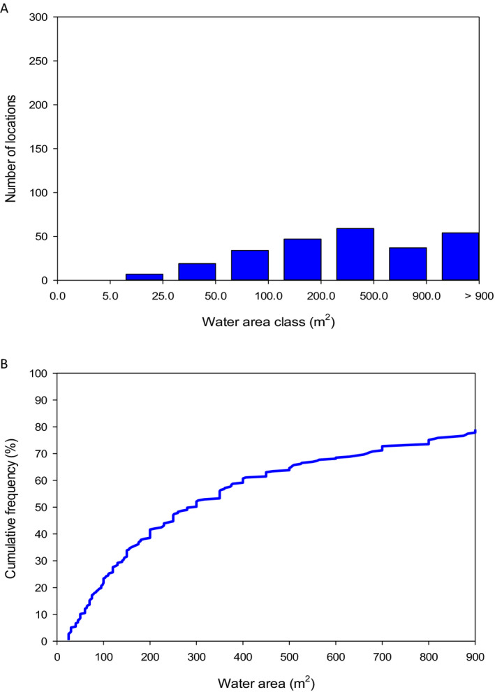
Frequency (A) and cumulative frequency distribution (B) of water surface area of 257 ponds in the UK. Note that in graph 7A the x‐axis is not linear and that all class boundaries are indicated. In graph 7B, ponds with a surface area greater than 900 m3 have not been included
Water volume
The water volume of the ponds was calculated by volume = mean depth × area. The frequency distributions are given for 109 records, for which a water depth was available. Figure 50 shows that 50 of the 109 ponds have a volume of less than 25 m3, 58 ponds a volume of less than 50 m3 (30 m3 is the minimum volume of the FOCUS ditches and streams) and that 107 of the 109 water bodies has a water volume of less than 900 m3 (the water volume of the FOCUS ponds). However, these numbers are largely biased, because for ponds with a mean water depth greater than 1 m, the water depths were not determined.
Figure 50.
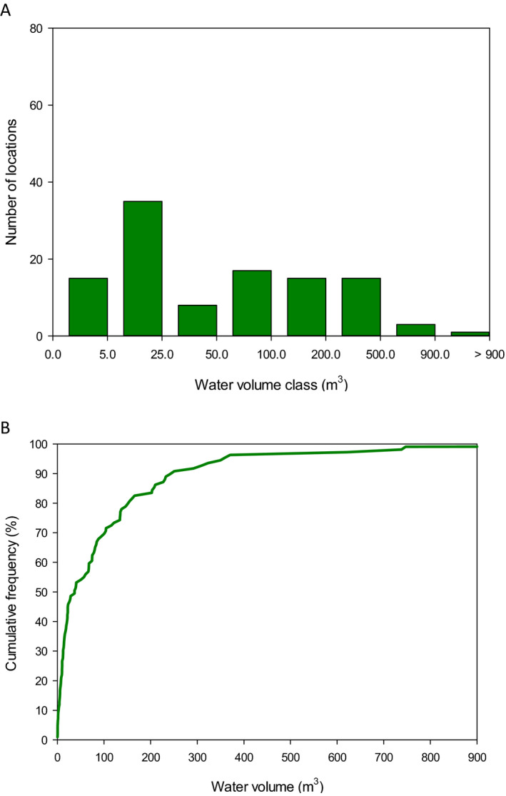
Frequency (A) and cumulative frequency (B) of water volume of 109 water bodies in the UK for which the water depth was determined, i.e. water bodies with depth < 1 m. Note that in graph A the x‐axis is not linear and that all class boundaries are indicated. In graph B, water bodies with a volume greater than 900 m3 have not been included
Surrounding land use
To obtain an idea about the surrounding land use of the ponds, the data base was analysed in two ways:
the recorded land use classification system according to the Institute of Terrestrial Ecology (Bunce et al., 1996a,b) was used to identify whether the pond was situated in a land use class in which arable land is well represented. Table 49 lists the ITE Land Class Number (2007) that we selected as containing significant areas of arable land use;
recorded surrounding land use percentage in two distance zones from the perimeter of the pond, 0–5 m and 0–100 m. Arable land use is one of the possible, listed categories (Murphy and Weatherby, 2008).
Table 49.
Land Class Number (without the England, Scotland or Wales indication) according to the ITE Land Class Number (2007) classification system with their description (Benefield et al., 1982) and our classification in arable land use or not
| Land class | Description of land use | Arable: yes/no |
|---|---|---|
| 1 | Cereals, good grasslands and limited native vegetation | Yes |
| 2 | Mainly good grassland, but extensive cereals and built up area | No |
| 3 | Cereals, other corps and short‐term grassland | Yes |
| 4 | Arable, with cereals and other crops, good grassland and urban | Yes |
| 5 | Mixed farmland although predominantly good grass; much urban | No |
| 6 | Mainly good grassland but with some barley | No |
| 7 | Mainly pasture with some arable and good grass | No |
| 8 | Mainly pasture with some arable, extensive mudflats and urban development | No |
| 9 | Mixture of good grass and arable with many urban areas | Yes |
| 10 | Mainly arable but with good grassland and pasture also widespread | Yes |
| 11 | Arable predominates particularly wheat with good grassland and urban | Yes |
| 12 | Arable, mainly wheat with limited food grassland and urban | Yes |
| 13 | Usually mixtures of arable and good grassland but also a variety of other uses | Yes |
| 14 | Mainly arable but also good grassland and much urban | Yes |
| 15 | Mainly pasture mixed with good land and arable | No |
| 16 | Varied with mixtures of arable pasture and good grassland | Yes |
| 17 | Mainly pastures with some good grassland | No |
| 18 | Predominantly rough grazing with some limited pasture land | No |
| 19 | Mainly rough grazing or forest, but some pasture | No |
| 20 | Much pasture, but some good grassland and occasional crops | No |
| 21 | Open range grazing or forest | No |
| 22 | Mainly rough grazing, but also woodland and occasional crops | No |
| 23 | Limited open range grazing | No |
| 24 | Limited open range grazing | No |
| 25 | Mainly barley, but with much good grassland | Yes |
| 26 | Mainly good grassland, but also much barley and pasture | No |
| 27 | Arable, particulary barley, but also much pasture and good grassland | Yes |
| 28 | Pasture or rough grazing predominate, but some good grasslands also | No |
| 29 | Mainly open range grazing, but also some crofting | No |
| 30 | Open range grazing and crofting | No |
| 31 | Manly rough grazing, but some good grassland and pasture with crofting | No |
| 32 | Mainly open range grazing, but some pasture | No |
On the basis of our classification of the ITE Land Class Number (Table 49), 115 of the 259 ponds were classified as being located in land‐use classes with significant arable land use. Of these 115 ponds, the water surface area was not recorded for two ponds. We made a frequency distribution for the remaining 113 ponds (Figure 51), which shows that all pond size classes have a comparable proportion of ponds with significant arable land use nearby. Small ponds with areas below 25 m2 were not included in the survey given the pond definition (required surface area of 25 m2 to 2 ha); the few that have been recorded appear to be predominantly situated in areas with non‐arable land use. The second way of land use classification resulted in 22 ponds that have a percentage of arable land in their 0–5 m distance zone and 59 ponds that have a percentage of arable land in their 0–100 m distance zone from the perimeter of the pond (17 of the 59 ponds were already included in the 22 ponds, having arable land in their 0–5 m distance zone). We made a frequency distribution for the 59 ponds (Figure 52), which shows that all pond size classes have a comparable proportion of ponds with arable land use in their 0–100 m perimeter. The percentage arable land use varies between 2% and 98%, for 3 of the 59 ponds the percentage was missing.
Figure 51.
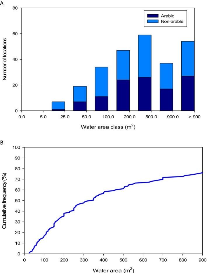
Frequency distribution (A) of water surface area of the 113 ponds in land use classes containing arable land use according to the ITE Land Class Number plus the 144 remaining ponds in the UK. Cumulative frequency distribution (B) is for the 113 ponds
Figure 52.
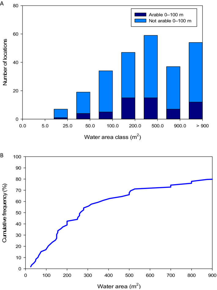
Frequency distribution (A) of water surface area of the 59 ponds in the UK where a percentage of arable land use was observed in the 0–100 m distance zone from the perimeter of the pond, plus the remaining 198 sampled ponds. Cumulative frequency distribution (B) is for the 59 ponds
As expected, comparison of Figures 51 and 52 shows that the more strict classification of arable land use present in the 0–100 m perimeter around the pond results in a smaller number of ponds with arable land use, than the regionally based land use classification using the ITE Land Class Number. The latter classification resulted in nearly 50% of the ponds being located in land use classes with significant arable land use (115 of the 259 ponds), while this was only approximately 20% for the former classification (59 of the 259 ponds).
Amphibians observed in ponds
The presence of amphibians was one of the recorded properties of the surveyed ponds. We expect the recorded number of ponds to represent an underestimation of the number of ponds hosting amphibians in reality, as the observation of amphibians will depend on the expertise on amphibians of the surveyor as well as on the time of the year of the survey (often between April/May to October/November).
In 49 ponds of the 259 sampled ponds, the presence of amphibians (e.g. tadpoles, frogs, newts) was observed. Except in the few sampled small ponds with areas below 25 m2, they were observed in ponds of all area classes (Figure 53). Of the 49 ponds with amphibians, 7 ponds have a percentage of arable land in their 0–5 m distance zone and 9 ponds have a percentage of arable land in their 0–100 m distance zone from the perimeter of the pond. In total, 19 of the 49 ponds were included in the 115 ponds which were classified as having significant arable land use according to the ITE Land Class Number. This indicates that a number of ponds having amphibians may probably receive pesticide residues via either spray‐drift deposition or runoff or drainage entries, Moreover, part of the ponds may have an inflow of water that may also carry pesticides into the ponds.
Figure 53.
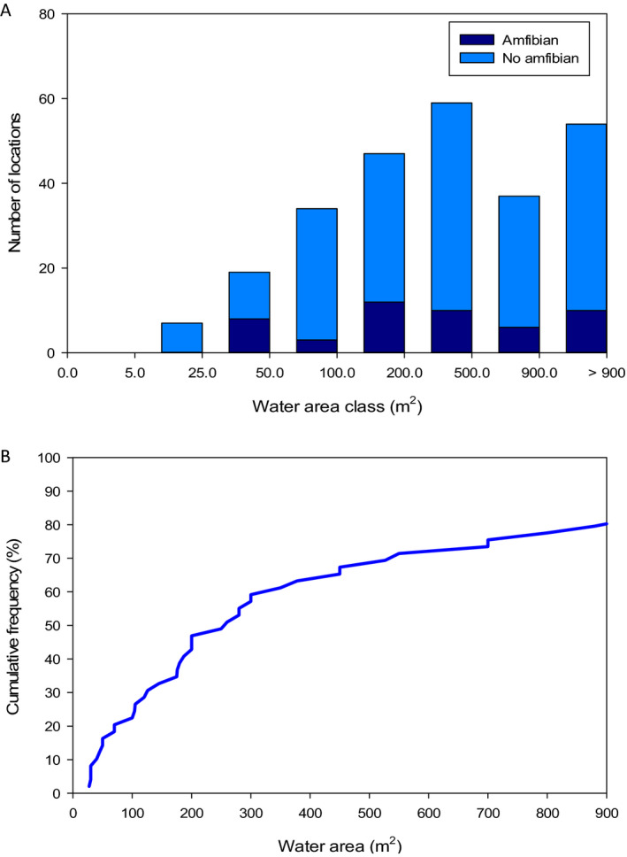
Frequency distribution (A) of water surface area of the 49 ponds in the UK where amphibians were observed, plus the remaining 208 sampled ponds. Cumulative frequency distribution (B) is for the 49 ponds where amphibians were observed
Comparison of analysed ponds and FOCUS water bodies
The analysis of water depth and water surface area (Table 50) of the Spanish and Swiss amphibian ponds (i.e. standing water bodies) and the CountrySide Survey ponds in the UK demonstrates that the most vulnerable 10% of them is considerably smaller than the FOCUS ponds: a water depth < 0.3 m vs the 1 m water depth of the FOCUS pond and a surface area < 100 m2 versus the 30 × 30 m = 900 m2 of the FOCUS pond. The smaller water depth and often smaller width imply that peak concentrations due to spray‐drift depositions will be significantly higher in the most vulnerable 10% of the analysed ponds than in the FOCUS pond (assuming all other factors equal, e.g. land use, distance edge‐of‐water to crop, spray‐drift deposition curves). So, the 90th‐percentile peak concentrations caused by spray‐drift deposition are expected to be significantly higher in the analysed ponds of Spain, Switzerland and the UK than in a FOCUS pond. Based upon the most vulnerable 10% water depth of less than 0.3 m and 10% water surface area of less than 100 m2, the most vulnerable 10% water volumes will be less than 300 m3. The water volumes of the most vulnerable 10% of the Spanish, Swiss and UK ponds are thus considerably smaller than the water volume of the FOCUS pond (900 m3) and this implies that peak concentrations due to drainage or runoff entries will be higher in the most vulnerable 10% of the analysed ponds than in the FOCUS pond (assuming similar drainage or runoff entries per m2 treated area and similar land:water ratios). Therefore, we expect the 90th percentile peak concentration caused by drainage or runoff entries to be significantly higher in the analysed ponds than in a FOCUS pond. Thus, our overall conclusion is that the FOCUS pond is not expected to result in conservative estimates of the peak exposure for amphibians in the analysed ponds of the three countries of Spain, Switzerland and the UK.
Table 50.
Overview of observed water depth (h) and water surface area (A) of the data for Spain, canton Aargau (Switzerland) and the UK
| Spain | Aargau (Switzerland) | UKa | |
|---|---|---|---|
| Number of water bodies | 794 | 729 | 259 |
| h | |||
| < 0.3 m | 18% | – | 27% |
| < 1.0 m | 70% | – | 42% |
| A | |||
| < 100 m2 | 59% | 52% | 23% |
| < 900 m2 | 87% | 89% | 79% |
No ponds of less than 25 m2 (although widely present in the UK landscape) or more than 2 ha. The presence of amphibians recorded at 19% (49/259) of the ponds, but is probably underestimated and has no bias versus water surface area (Figure 52A).
Comparing the peak concentrations in the analysed water ponds to those in FOCUS ditches and streams is more complicated; therefore, we are unable to make a statement on the conservativeness of peak concentrations in FOCUS ditches and streams for the analysed ponds. For spray‐drift‐related peaks, we have to consider that spray‐drift depositions on the FOCUS ditch and stream are expected to be considerably higher than the deposition on the analysed ponds, because of the relatively short distances from crop to edge of water and the narrow 1‐m wide water surface areas for FOCUS ditches and streams. However, water depths in the analysed ponds may be higher than the minimum water depth of 0.30 m in FOCUS ditches and streams, so this might countervail the higher deposited areic pesticide mass, although probably not to the same extent as the two factors mentioned above. So, spray‐drift‐related peaks might be higher in FOCUS ditches and streams. For runoff‐related or drainage‐related peaks, it is not possible to compare the initial water volume in the analysed ponds versus the volume of the FOCUS ditches and streams, while also the land:water ratio of the analysed ponds is unknown. Furthermore, the role of the upstream located fields (2 ha untreated for FOCUS ditch and 100 ha of which 20 ha treated for FOCUS stream) complicates the comparison, and thus, we are unable to draw a conclusion on the conservativeness of the peak exposure for amphibians in the analysed ponds.
However, in view of the higher flow‐through rates in the FOCUS ditches and streams, the pesticide concentrations are expected to remain for considerable longer periods in the analysed ponds than in FOCUS ditches and streams, and thus, the chronic exposure in the analysed ponds is probably underestimated. So, for the chronic risk assessment we expect that the FOCUS ditches and streams are not conservative.
References
Benefield CB and Bunce RGH, 1982. A preliminary visual presentation of land classes in Britain. Grange‐over‐Sands, Institute of Terrestrial Ecology, 39 pp. (Merlewood Research and Development Paper No. 91)
Bunce RGH, Barr CJ, Clarke RT, Howard DC and Lane AMJ, 1996a. ITE Merlewood Land Classification of Great Britain. Journal of Biogeography, 23, 625–634.
Bunce RGH, Barr CJ, Clarke RT, Howard DC and Lane AMJ, 1996b. Land classification for strategic ecological survey. Journal of Environmental Management, 47, 37–60.
Murphy J and Weatherby A, 2008. Countryside Survey. Freshwater Manual. CS technical report No. 5/07 (www.countrysidesurvey.org.uk).
Williams P, Biggs J, Crowe A, Murphy J, Nicolet P, Weatherby A and Dunbar M, 2010. Countryside Survey. Ponds Report from 2007. CS technical report No. 7/07 (www.countrysidesurvey.org.uk).
Appendix D – Brief description of Step 3 FOCUS surface water scenarios to predict exposure in the aquatic environment
1.
In order to predict the exposure to PPP in surface waters, different models may be used. The exposure assessment for the aquatic environment in the EU is currently based on the FOCUS methodology (FOCUS, 2014). It is a step‐by‐step procedure for the calculation of PECs in surface water. The procedure consists of four steps. In steps 1 and 2, the water body is static with a depth of 30 cm and a 5 cm deep sediment layer with 5% organic carbon. The width of the water body is not relevant in steps 1 and 2. In step 3, the water body is either a ditch, pond or stream adjacent to a single pesticide‐treated field. The step 3 water bodies receive spray‐drift deposition, entries via runoff or eroded soil particles and entries by drain pipes. The pesticide input in a water body by spray‐drift deposition is determined by its distance to the treated field. For pesticide entries via runoff/erosion, the size of the contributing area is relevant and the same holds for drainage entries. FOCUS ditches, streams as well as ponds may be fed by runoff/erosion or drainage. Streams are fed by a small pesticide‐free base flow plus discharge from an upstream located catchment of 100 ha, of which 20 ha are assumed to be treated with pesticide. Ditches are fed by a small pesticide‐free base flow plus the discharge of two upstream fields of 1 ha each, assumed to be not‐treated. Ponds are fed by a small pesticide‐free base flow plus the discharge of a surrounding area of 4,500 m2, which is treated (and spray drift deposition coming in from one 30‐m long side). All ditches and streams are assumed to have a length of 100 m, a width of 1 m and a variable, but minimum depth of 30 cm, flow rates are up to 3,100 m/day for ditches and 28,800 m/day for streams.
Ponds are defined by surface water areas of 30 × 30 m together with a depth of 100 cm with generally low discharges of approximately 0.025–0.1 L/s, raising up to 0.4–1.6 L/s after runoff entries (FOCUS, 2014). This methodology was developed to predict a realistic worst‐case exposure of fish, aquatic invertebrates and algae.
The FOCUS surface water scenarios were developed as a third step in a stepwise approach to calculate predicted environmental concentrations (PECsw) in 10 ‘realistic worst‐case’ scenarios (FOCUS, 2014). The scenarios cover a realistic range of surface water bodies, topography, climate, crops, soil types and agricultural management practices in the major agricultural areas of the EU. Their worst‐casedness is mainly based upon the assessment of worst‐casedness of the pesticide entry routes, statistical methods following the criteria mentioned for the Exposure Assessment Goals of Section 9 were not yet developed. The scenarios intend to represent ‘realistic worst‐case’ scenarios for the PECs (dissolved concentration) in the water layer and not for the PECs in sediment. Ponds figure in only 3 of the 10 FOCUS scenarios (Table 51 and Figures 54, 55 and 56) and thus, they do not cover large parts of the EU, especially in southern Europe. Moreover, as the FOCUS surface water scenarios have been designed in the late nineties of the former century, the newer MS, including many eastern European MS were not considered in the scenario development procedure and thus these are not covered as well. Generally speaking, for an active substance to pass, the risk assessment the pond as well as the stream and ditch scenario needs to be passed.
Table 51.
Overview of FOCUS surface water scenarios with their code D or R (indicating that either drainage or runoff+erosion is the main entry route for pesticides, next to spray drift deposition), their associated water body types and meteorological station
| Scenario code | Type of water bodies | Meteorological station |
|---|---|---|
| D1 | Ditch, stream | Lanna, Sweden |
| D2 | Ditch, stream | Brimstone, UK |
| D3 | Ditch | Vredepeel, Netherlands |
| D4 | Pond, stream | Skousbo, Denmark |
| D5 | Pond, stream | La Jaillière, France |
| D6 | Ditch | Thiva, Greece |
| R1 | Pond, stream | Weiherbach, Germany |
| R2 | Stream | Porto, Portugal |
| R3 | Stream | Bologna, Italy |
| R4 | Stream | Roujan, France |
Figure 54.
Extent of FOCUS surface water scenario D4 in the EU15 that includes ponds (source: FOCUS SWASH 5.3)
Figure 56.
Extent of FOCUS surface water scenario R1 in the EU15 that includes ponds (source: FOCUS SWASH 5.3)
At present, the main limitation of the FOCUS surface water scenarios is that they consider only one year, which may result in unreliable estimates of 90th percentile exposure concentrations, leading to an underestimation of risks for the aquatic ecosystem. Considering exposure in FOCUS ponds, a limitation is that evaporation of the water in the pond is not taken into account and thus the water level is always around 1 m, which is relatively deep compared to shallow temporary water bodies which are a preferred habitat for the majority of amphibians.
Figure 55.
Extent of FOCUS surface water scenario D5 in the EU15 that includes ponds (source: FOCUS SWASH 5.3)
Reference
FOCUS, 2014. “FOCUS Surface Water Scenarios in the EU Evaluation Process under 91/414/EEC”. Report of the FOCUS Working Group on Surface Water Scenarios, EC Document Reference SANCO/4802/2001‐rev.2. 245 pp.
Appendix E – Type and size of water body preferred for breeding by different amphibian species
1.
Surface area of breeding sites
From a summary of data from literature data on breeding sites was extracted and used for descriptive statistics. Minimum and maximum values as well as means and medians for different amphibian species were determined and displayed in Figure 57. Data was retrieved from studies, where it was explicitly specified that ponds were used as breeding‐sites or wherever the presence of juveniles, tadpoles, or eggs were reported.
Figure 57.
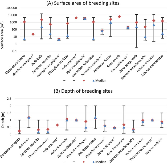
Ranges of surface area (A) and depth measurements (B) of breeding sites reported in literature for different amphibian species. Medians (blue triangle) and means (red diamond) were calculated from literature values for n ≧ 2. Species for which only two data points were available are marked with a °; species for which only a single mean value was reported are marked with a*
Surface size measurements for sites, in which the use as breeding site was not explicitly stated or only the presence of adults was reported, were not considered for this graph. The retrieved data consisted out of measurements of single ponds and mean values for several ponds described in one study. If for one species, both mean values and single values were reported in several studies, means were treated as single measurements for descriptive statistics when summarising all studies. Then, for calculation of means, the reported mean values were not weighted by the number of ponds but treated as single values since sites were not randomly chosen in the studies. This was done to not falsely inflate the descriptive statistics by giving too much power to the mean values of selected sites. Instead, they were treated as single pond measurements and used for calculations of arithmetic means. If only one mean value was reported for a species, the mean value was displayed and species were marked with a * in Figure 57.
Surface area and depth data could be evaluated for 17 and 16 species, respectively. Median surface areas ranged from 4.50 to 3,500 m2 for Discoglossus galganoi (n = 3) and Hyla meridionalis (n = 2), respectively (Garcia‐Gonzalez & Garcia‐Vazquez 2012; Ruhi et al., 2012). The smallest median depth was reported for Discoglossus pictus (n = 10) and Epidaelea calamita (n = 14) with 0.18 m (Ruhi et al., 2012; Sebastian et al., 2015). Maximum median depth values were reported for Bufo bufo (n = 6) and Pelobates fuscus (n = 5) with 1.20 m, respectively (Eggert and Guyetant 1999; Nystrom et al., 2007; Ruhi et al., 2012; Sebasti and Carpaneto 2004; Sztatecsny and Holdl 2009). The compiled data can aid to add certainty to the characterisation of breeding habitats. The data gives a rough estimate of the ranges of breeding pond sizes within which species occurred, but does not rule out that habitats of different sizes might also be suitable for the respective species.
List of Publications that were used to answer the research question and from which data was retrieved
Berger G, Graef F and Pfeffer H, 2012. Temporal coincidence of migrating amphibians with mineral fertiliser applications on arable fields. Agriculture Ecosystems & Environment, 155, 62–69. https://doi.org/10.1016/j.agee.2012.04.006
Berger G, Graef F and Pfeffer H, 2013. Glyphosate applications on arable fields considerably coincide with migrating amphibians. Scientific Reports, 3, 2622. https://doi.org/10.1038/srep02622
Burghelea C, Zaharescu D and Palanca A, 2013. Phenotypic indicators of developmental instability in an endemic amphibian from an altered landscape (Monegros, NE Spain). Amphibia‐Reptilia, 34, 505–516. https://doi.org/10.1163/15685381-00002908
Burghelea CI, Zaharescu DG and Palanca‐Soler A, 2010. Dietary overview of Pelophylax perezi from Monegros rice fields (northeast Spain). Herpetological Journal, 20, 219–224.
Cayuela H, Besnard A and Joly P, 2013. Multi‐event models reveal the absence of interaction between an invasive frog and a native endangered amphibian. Biological Invasions, 15, 2001–2012. https://doi.org/10.1007/s10530-013-0427-x
Chadwick EA, Slater FM and Ormerod SJ, 2006. Inter‐ and intraspecific differences in climatically mediated phenological change in coexisting Triturus species. Global Change Biology, 12, 1069–1078. https://doi.org/10.1111/j.1365-2486.2006.01156.x
Covaciu‐Marcov SD, Cicort‐Lucaciu AS, Mitrea I, Sas I, Caus AV and Cupsa D, 2010. Feeding of three syntopic newt species (Triturus cristatus, Mesotriton alpestris and Lissotriton vulgaris) from Western Romania. North‐Western Journal of Zoology, 6, 95–108.
Cox NA and Temple HJ, 2009. European Red List of Reptiles. Luxembourg: Office for Offcial Publications of the European Communities.
Curado N, Hartel T and Arntzen JW, 2011. Amphibian pond loss as a function of landscape change ‐ A case study over three decades in an agricultural area of northern France. Biological Conservation, 144, 1610–1618. https://doi.org/10.1016/j.biocon.2011.02.011
Dalbeck L, Janssen J and Volsgen SL, 2014. Beavers (Castor fiber) increase habitat availability, heterogeneity and connectivity for common frogs (Rana temporaria). Amphibia‐Reptilia, 35, 321–329. https://doi.org/10.1163/15685381-00002956
Dalbeck L, Luscher B and Ohlhoff D, 2007. Beaver ponds as habitat of amphibian communities in a central European highland. Amphibia‐Reptilia, 28, 493–501. https://doi.org/10.1163/156853807782152561
Dalbeck L and Weinberg K, 2009. Artificial ponds: a substitute for natural Beaver ponds in a Central European Highland (Eifel, Germany)? Hydrobiologia, 630, 49–62. https://doi.org/10.1007/s10750-009-9779-8
Deeming DC, 2008. Capture of smooth newts (Lissotriton vulgaris) and great crested newts (Triturus cristatus) correlates with the lunar cycle. The Herpetological Journal, 18, 171–174.
Denoel M and Ficetola GF, 2008. Conservation of newt guilds in an agricultural landscape of Belgium: the importance of aquatic and terrestrial habitats. Aquatic Conservation‐Marine and Freshwater Ecosystems, 18, 714–728. https://doi.org/10.1002/aqc.853
Dervo BK, Baerum KM, Skurdal J and Museth J, 2016. Effects of Temperature and Precipitation on Breeding Migrations of Amphibian Species in Southeastern Norway. Scientifica. https://doi.org/10.1155/2016/3174316
Edgar PW, Griffiths RA and Foster JP, 2005. Evaluation of translocation as a tool for mitigating development threats to great crested newts (Triturus cristatus) in England, 1990–2001. Biological Conservation, 122, 45–52. https://doi.org/10.1016/j.biocon.2004.05.022
Eggert C and Guyetant R, 1999. Age structure of a spadefoot toad Pelobates fuscus (Pelobatidae) population. Copeia 4, 1127–1130. https://doi.org/10.2307/1447991
Eibl‐Eibesfeldt I, xe and us, 1950. Ein Beitrag zur Paarungsbiologie der Erdkröte (Bufo bufo L.). Behaviour, 2, 217–236.
Fasola M, 1993. Resource partitioning by 3 species of newts during their aquatic phase. Ecography, 16, 73–81. https://doi.org/10.1111/j.1600-0587.1993.tb00060.x
Fischer K, Becker M, Becker BA, Bensch J, Bockers A, Burmeister M, … Winter M, 2015. Determinants of tree frog calling ponds in a human‐transformed landscape. Ecological Research, 30, 439–450. https://doi.org/10.1007/s11284-014-1238-y
Fretey T, Cam E, Le Garff B and Monnat JY, 2004. Adult survival and temporary emigration in the common toad. Canadian Journal of Zoology‐Revue Canadienne De Zoologie, 82, 859–872. https://doi.org/10.1139/z04-058
Garcia‐Gonzalez C and Garcia‐Vazquez E, 2012. Urban Ponds, Neglected Noah's Ark for Amphibians. Journal of Herpetology, 46, 507–514. https://doi.org/10.1670/10-227
Griffiths RA, Dewijer P and May RT, 1994. Predation and competition within an assemblage of larval newts (triturus). Ecography, 17, 176–181. https://doi.org/10.1111/j.1600-0587.1994.tb00091.x
Grozinger F, Thein J, Feldhaar H and Rodel MO, 2014. Giants, dwarfs and the environment ‐ metamorphic trait plasticity in the common frog. Plos One, 9, 11. https://doi.org/10.1371/journal.pone.0089982
Grozinger F, Wertz A, Thein J, Feldhaar H and Rodel MO, 2012. Environmental factors fail to explain oviposition site use in the European common frog. Journal of Zoology, 288, 103–111. https://doi.org/10.1111/j.1469-7998.2012.00929.x
Gustafson DH, Andersen ASL, Mikusinski G and Malmgren JC, 2009. Pond Quality Determinants of Occurrence Patterns of Great Crested Newts (Triturus cristatus). Journal of Herpetology, 43, 300–310.
Gustafson DH, Malmgren JC and Mikusinski G, 2011. Terrestrial habitat predicts use of aquatic habitat for breeding purposes ‐ a study on the great crested newt (Triturus cristatus). Annales Zoologici Fennici, 48, 295–307.
Hangartner S, Laurila A and Rasanen K, 2011. Adaptive divergence of the moor frog (Rana arvalis) along an acidification gradient. Bmc Evolutionary Biology, 11, 12. https://doi.org/10.1186/1471-2148-11-366
Hartel T, Moga CI, Ollerer K and Puky M, 2009. Spatial and temporal distribution of amphibian road mortality with a Rana dalmatina and Bufo bufo predominance along the middle section of the Tarnava Mare basin, Romania. North‐Western Journal of Zoology, 5, 130–141.
Hartel T, Nemes S and Mara G, 2007. Breeding phenology and spatio‐temporal dynamics of pond use by the yellow‐bellied toad (Bombina variegata) population: the importance of pond availability and duration. Acta Zoologica Lituanica, 17, 56–63.
Hartel T and von Wehrden H, 2013. Farmed areas predict the distribution of amphibian ponds in a traditional rural landscape. Plos One, 8, 8. https://doi.org/10.1371/journal.pone.0063649
Hoffmann A, Tietje GA and Reyer HU, 2015. Spatial behavior in relation to mating systems: movement patterns, nearest‐neighbor distances, and mating success in diploid and polyploid frog hybrids (Pelophylax esculentus). Behavioral Ecology and Sociobiology, 69, 501–517. https://doi.org/10.1007/s00265-014-1862-0
Huste A, Clobert J and Miaud C, 2006. The movements and breeding site fidelity of the natterjack toad (Bufo calamita) in an urban park near Paris (France) with management recommendations. Amphibia‐Reptilia, 27, 561–568. https://doi.org/10.1163/156853806778877130
Jakob C, Miaud C, Crivelli AJ and Veith M, 2003. How to cope with periods of drought? Age at maturity, longevity, and growth of marbled newts (Triturus marmoratus) in Mediterranean temporary ponds. Canadian Journal of Zoology‐Revue Canadienne De Zoologie, 81, 1905–1911. https://doi.org/10.1139/z03-164
Jehle R and Arntzen JW, 2000. Post‐breeding migrations of newts (Triturus cristatus and T. marmoratus) with contrasting ecological requirements. Journal of Zoology, 251, 297–306. https://doi.org/10.1111/j.1469-7998.2000.tb01080.x
Jehle R, Arntzen W, Burke T, Krupa AP and Hodl W, 2001. The annual number of breeding adults and the effective population size of syntopic newts (Triturus cristatus, T. marmoratus). Molecular Ecology, 10, 839–850. https://doi.org/10.1046/j.1365-294x.2001.01237.x
Jofre GM, Warn MR and Reading CJ, 2016. The role of managed coniferous forest in the conservation of reptiles. Forest Ecology and Management, 362, 69–78. https://doi.org/10.1016/j.foreco.2015.11.044
Johansson M, Rasanen K and Merila J, 2001. Comparison of nitrate tolerance between different populations of the common frog, Rana temporaria. Aquatic Toxicology, 54, 1–14. https://doi.org/10.1016/s0166-445x(00)00182-x
Kopecky O, Vojar J, Susta F and Rehak I, 2011. Non‐prey items in stomachs of alpine newts (Mesotriton alpestris, Laurenti). Polish Journal of Ecology, 59, 631–635.
Kovar R, Brabec M, Vita R and Bocek R, 2009. Spring migration distances of some Central European amphibian species. Amphibia‐Reptilia, 30, 367–378.
Laugen AT, Laurila A, Rasanen K and Merila J, 2003. Latitudinal counter gradient variation in the common frog (Rana temporaria) development rates ‐ evidence for local adaptation. Journal of Evolutionary Biology, 16, 996–1005. https://doi.org/10.1046/j.1420-9101.2003.00560.x
Laurila A, 1998. Breeding habitat selection and larval performance of two anurans in freshwater rock‐pools. Ecography, 21, 484–494. https://doi.org/10.1111/j.1600-0587.1998.tb00440.x
Lenhardt PP, Bruhl CA and Berger G, 2015. Temporal coincidence of amphibian migration and pesticide applications on arable fields in spring. Basic and Applied Ecology, 16, 54–63. https://doi.org/10.1016/j.baae.2014.10.005
Lenhardt PP, Schafer RB, Theissinger K and Bruhl CA, 2013. An expert‐based landscape permeability model for assessing the impact of agricultural management on amphibian migration. Basic and Applied Ecology, 14, 442–451. https://doi.org/10.1016/j.baae.2013.05.004
Lizana M, Marquez R and Martinsanchez R, 1994. Reproductive‐biology of pelobates‐cultripes (anura, pelobatidae) in central Spain. Journal of Herpetology, 28, 19–27. https://doi.org/10.2307/1564675
Madsen T, 1984. Movements, home range size and habitat use of radio‐tracked grass snakes (natrix‐natrix) in Southern Sweden. Copeia, 3, 707–713.
Marty P, Angelibert S, Giani N and Joly P, 2005. Directionality of pre‐ and post‐breeding migrations of a marbled newt population (Triturus marmoratus): implications for buffer zone management. Aquatic Conservation‐Marine and Freshwater Ecosystems, 15, 215–225. https://doi.org/10.1002/aqc.672
Meek R, 2012. Patterns of amphibian road‐kills in the Vendee region of Western France. Herpetological Journal, 22, 51–58.
Miaud C, Joly P and Castanet J, 1993. Variation in age structures in a subdivided population of triturus‐cristatus. Canadian Journal of Zoology‐Revue Canadienne De Zoologie, 71, 1874–1879. https://doi.org/10.1139/z93-267
Miaud C and Sanuy D, 2005. Terrestrial habitat preferences of the natterjack toad during and after the breeding season in a landscape of intensive agricultural activity. Amphibia‐Reptilia, 26, 359–366. https://doi.org/10.1163/156853805774408496
Miaud C, Sanuy D and Avrillier JN, 2000. Terrestrial movements of the natterjack toad Bufo calamita (Amphibia, Anura) in a semi‐arid, agricultural landscape. Amphibia‐Reptilia, 21, 357–369. https://doi.org/10.1163/156853800507426
Nystrom P, Hansson J, Mansson J, Sundstedt M, Reslow C and Brostrom A, 2007. A documented amphibian decline over 40 years: Possible causes and implications for species recovery. Biological Conservation, 138, 399‐411. https://doi.org/10.1016/j.biocon.2007.05.007
Nystrom P, Svensson O, Lardner B, Bronmark C and Graneli W, 2001. The influence of multiple introduced predators on a littoral pond community. Ecology, 82, 1023–1039. https://doi.org/10.1890/0012-9658(2001)082[1023:tiomip]2.0.co;2
O'Brien CD, 2015. Sustainable drainage system (SuDS) ponds in Inverness, UK and the favourable conservation status of amphibians. Urban Ecosystems, 18, 321–331. https://doi.org/10.1007/s11252-014-0397-5
Rannap R, Lohmus A and Briggs L, 2009. Restoring ponds for amphibians: a success story. Hydrobiologia, 634, 87–95. https://doi.org/10.1007/s10750-009-9884-8
Reading CJ, 2010. The impact of environmental temperature on larval development and metamorph body condition in the common toad, Bufo bufo. Amphibia‐Reptilia, 31, 483–488. https://doi.org/10.1163/017353710x521537
Reinhardt T, Steinfartz S, Paetzold A and Weitere M, 2013. Linking the evolution of habitat choice to ecosystem functioning: direct and indirect effects of pond‐reproducing fire salamanders on aquatic‐terrestrial subsidies. Oecologia, 173, 281–291. https://doi.org/10.1007/s00442-013-2592-0
Reinhardt T, Steinfartz S and Weitere M, 2015. Inter‐annual weather variability can drive the outcome of predator prey match in ponds. Amphibia‐Reptilia, 36, 97–109. https://doi.org/10.1163/15685381-00002982
Reques R and Tejedo M, 1995. Negative correlation between length of larval period and metamorphic size in natural‐populations of natterjack toads (bufo‐calamita). Journal of Herpetology, 29, 311–314. https://doi.org/10.2307/1564576
Rogell B, Hofman M, Eklund M, Laurila A and Hoglund J, 2009. The interaction of multiple environmental stressors affects adaptation to a novel habitat in the natterjack toad Bufo calamita. Journal of Evolutionary Biology, 22, 2267–2277. https://doi.org/10.1111/j.1420-9101.2009.01842.x
Ruhi A, Sebastian OS, Feo C, Franch M, Gascon S, Richter‐Boix A and Llorente G, 2012. Man‐made Mediterranean temporary ponds as a tool for amphibian conservation. Annales De Limnologie‐International Journal of Limnology, 48, 81–93. https://doi.org/10.1051/limn/2011059
Sebasti S and Carpaneto GM, 2004. An ecological study on amphibian communities inhabiting the dewponds of a lowland deciduous forest along the Tyrrhenian coast (central Italy). Italian Journal of Zoology, 71, 135–141. https://doi.org/10.1080/11250000409356622
Sebastian OS, Navarro J, Llorente GA and Richter‐Boix A, 2015. Trophic Strategies of a Non‐Native and a Native Amphibian Species in Shared Ponds. Plos One, 10, 17. https://doi.org/10.1371/journal.pone.0130549
Shakhparonov VV, 2011. Patterns of Orientation Behavior in Marsh Frogs (Rana ridibunda Pall.) of Southern Populations. Biology Bulletin, 38, 528–532. https://doi.org/10.1134/s1062359011050116
Simon E, Puky M, Braun M and Tothmeresz B, 2012. Assessment of the effects of urbanization on trace elements of toe bones. Environmental Monitoring and Assessment, 184, 5749–5754. https://doi.org/10.1007/s10661-011-2378-y
Sinsch U and Leskovar C, 2011. Does thermoregulatory behaviour of green toads (Bufo viridis) constrain geographical range in the west? A comparison with the performance of syntopic natterjacks (Bufo calamita). Journal of Thermal Biology, 36, 346–354. https://doi.org/10.1016/j.jtherbio.2011.06.012
Skei JK, Dolmen D, Ronning L and Ringsby TH, 2006. Habitat use during the aquatic phase of the newts Triturus vulgaris (L.) and T. cristatus (Laurenti) in central Norway: proposition for a conservation and monitoring area. Amphibia‐Reptilia, 27, 309–324. https://doi.org/10.1163/156853806778189972
Strong RJ, Halsall CJ, Ferencik M, Jones KC, Shore RF and Martin FL, 2016. Biospectroscopy reveals the effect of varying water quality on tadpole tissues of the common frog (Rana temporaria). Environmental Pollution, 213, 322–337. https://doi.org/10.1016/j.envpol.2016.02.025
Sztatecsny M and Hodl W, 2009. Can protected mountain areas serve as refuges for declining amphibians? Potential threats of climate change and amphibian chytridiomycosis in an alpine amphibian population. Eco Mont‐Journal on Protected Mountain Areas Research, 1, 19–24.
Tejedo M, 1992. Effects of body size and timing of reproduction on reproductive success in female natterjack toads (Bufo calamita). Journal of Zoology, 228, 545–555.
Tejedo M, 1993. Size‐dependent vulnerability and behavioral‐responses of tadpoles of 2 anuran species to beetle larvae predators. Herpetologica, 49, 287–294.
Temple HJ and Cox NA, 2009. European Red List of Amphibians. Luxembourg: Office for Official Publications of the European Communities.
Van Buskirk J and Arioli M, 2005. Habitat specialization and adaptive phenotypic divergence of anuran populations. Journal of Evolutionary Biology, 18, 596–608. https://doi.org/10.1111/j.1420-9101.2004.00869.x
Vignoli L, D'Amen M, Della Rocca F, Bologna MA and Luiselli L, 2014. Contrasted influences of moon phases on the reproduction and movement patterns of four amphibian species inhabiting different habitats in central Italy. Amphibia‐Reptilia, 35, 247–254. https://doi.org/10.1163/15685381-00002943
Vences M, Puente M, Nieto S and Vieites DR, 2002. Phenotypic plasticity of anuran larvae: environmental variables influence body shape and oral morphology in Rana temporaria tadpoles. Journal of Zoology, 257, 155–162. https://doi.org/10.1017/s0952836902000754
Vos CC and Chardon JP, 1998. Effects of habitat fragmentation and road density on the distribution pattern of the moor frog Rana arvalis. Journal of Applied Ecology, 35, 44–56.
Vuorio V, Heikkinen RK and Tikkanen OP, 2013. Breeding success of the threatened great crested newt in boreal forest ponds. Annales Zoologici Fennici, 50, 158–169.
Weitere M, Tautz D, Neumann D and Steinfartz S, 2004. Adaptive divergence vs. environmental plasticity: tracing local genetic adaptation of metamorphosis traits in salamanders. Molecular Ecology, 13, 1665–1677. https://doi.org/10.1111/j.1365-294x.2004.02155.x
Wilkinson JW, Beebee TJC and Griffiths RA, 2007. Conservation genetics of an island toad: Bufo bufo in Jersey. Herpetological Journal, 17, 192–198.
Appendix F – Toxicity studies and available endpoints for fish and sediment dwellers
1.
Acute toxicity to fish
Acute Toxicity Test (OECD 203, exposure for 96 h)
Mortalities are recorded at 24, 48, 72 and 96 h and the concentrations, which kill 50% of the fish (LC50), are determined where possible.
Long‐term and chronic toxicity to fish
Prolonged toxicity test (OECD 204, exposure for 14 days)
Threshold levels of lethal and other observed effects and NOEC are determined at intervals during the test period, which is at least 14 days. Observed effects other than lethal effects are on the appearance, size and behaviour of the fish, e.g. different swimming behaviour, different reaction to external stimuli, reduction or cessation of food intake.
Fish early life stage toxicity test (OECD 210, exposure from fertilised egg to free‐feeding)
Tests with the early life stages of fish are intended to define the lethal and sublethal effects of chemicals on the stages and species tested. Observed effects are cumulative mortality, numbers of healthy fish at end of test, time to start of hatching and end of hatching, numbers of larvae hatching each day, length and weight of surviving animals, numbers of deformed larvae, numbers of fish exhibiting abnormal behaviour. Reproduction is not measured in this test.
Juvenile growth test (OECD 215, exposure 28 days)
This test is designed to assess the effects of prolonged exposure to chemicals on the growth of juvenile fish. Observed effects are external abnormalities (such as haemorrhage, discolouration), abnormal behaviour, weight and mortality.
Short‐term reproduction assay (OECD 229, exposure 21 days)
A fish assay capable of detecting endocrine active substances. Vitellogenin and secondary sexual characteristics are the two biomarkers, which are measured in addition to an evaluation of quantitative egg production (fecundity) and a performance of gonadal histopathology. Additionally, abnormal behaviour (such as hyperventilation, uncoordinated swimming, loss of equilibrium and atypical quiescence or feeding), external abnormalities (such as haemorrhage, discolouration), territorial aggressiveness, appearance of the fish and mortality are noted.
Fish full life cycle test (EPA)
In the fish life cycle toxicity test, fish are cultured in the presence of the test substance from one stage of the life cycle to at least the same stage of the next generation (e.g. egg to egg) this leads to study durations of 100–190 days, depending on the selected fish species. The test covers the hatching of larvae, a growth phase of juvenile fish and reproduction. Once the fish are mature and start spawning, the egg number and fertilisation rate is documented. The hatching success and survival of the F1 generation is evaluated. During the test period, the fish of the parental and F1 generation are observed daily for survival, hatching, abnormal appearance and behaviour. Length, weight and sex ratio are evaluated at the end of the test and of those fish being removed from the test. During the reproductive phase, coagulated and fertilised eggs are counted. Additionally, at the end of the test the vitellogenin level, which is an egg yolk precursor produced in the liver as response of circulation endogenous oestrogen (of blood or tissue sample), is measured. Furthermore, the sex ratio is analysed and a histopathology is performed.
Bioconcentration in fish (OECD 305)
The test consists of two phases: the exposure (uptake) and post‐exposure (depuration) phases. The uptake rate constant, the depuration (loss) rate constant (or constants, where more complex models are involved), the bioconcentration factor, and where possible, the confidence limits of each of these parameters are calculated from the model that best describes the measured concentrations of test substance in fish and water.
Long‐term and chronic toxicity to sediment dwelling invertebrates
Sediment‐water chironomid toxicity test using spiked sediment (OECD 218, exposure for 28, resp. 65 days)
First instar chironomid larvae are exposed in a water–sediment system to spiked sediment. Chironomid emergence and development rate is measured at the end of the test. The exposure of the chironomid larvae is expected to mainly occur via the pore water.
Sediment‐water chironomid toxicity test using spiked water (OECD 219, exposure for 28, resp. 65 days)
First instar chironomid larvae are exposed in a water–sediment system to spiked water. The measured endpoints are the total number of adults emerged and the time to emergence.
Sediment‐water lumbriculus toxicity test using spiked sediment (OECD 225, exposure 28 days)
Lumbriculus variegatus burrows in the spiked sediment and ingests sediment particles below the sediment surface. This ensures exposure of the test organisms to the test substance via all possible uptake routes (e.g. contact with, and ingestion of contaminated sediment particles, but also via porewater and overlying water). Effects on reproduction and the biomass of the test organisms are recorded.
Further information on testing of sediment dwelling organisms can be found in EFSA PPR Panel, 2016c
Reference
EFSA PPR Panel (EFSA Panel on Plant Protection Products and their Residues), 2015b. Scientific Opinion on the effect assessment for pesticides on sediment organisms in edge‐of‐field surface water.
Appendix G – Oral and dermal exposure calculations
1.
Introduction
Worst‐case exposure calculations were conducted in order to:
compare the relative importance of oral and dermal exposure pathways
identify the groups of amphibians and reptiles with the greatest oral and dermal exposure
investigate whether the exposure estimates in first‐tier risk assessment for birds and mammals cover amphibians and reptiles (only for oral exposure)
The results should help to focus the efforts to the most important exposure pathways.
The oral exposure was calculated for small‐, medium‐ and large‐sized amphibians and reptiles weighting 1.4, 11 and 100 g in order to find out which of the groups of organisms are most exposed. For tortoises, oral exposure was calculated for animals of 11, 100 and 1,000 g of weight. The weight of tortoise at hatching ranges from 9.6 to 12.7 g (Bertolero et al. 2011), and hence, it was considered not meaningful to calculate oral exposure of a tortoise weighting only 1.4 g.
An application rate of 1 kg a.s./ha is assumed in the oral and dermal exposure calculations for easy comparisons between the different orders of vertebrates and routes of exposure.
Oral exposure via food uptake
The oral exposure is calculated with generic residues values (RUD) for different food items from the EFSA birds and mammals guidance (EFSA 2015a), Appendix F, table 1 (http://onlinelibrary.wiley.com/doi/10.2903/j.efsa.2009.1438/full).
The 90th percentile RUD values were used. These are the standard RUDs used in the first‐tier acute risk assessment for birds and mammals.
Amphibians
The estimated theoretical exposure (ETE) was calculated in Table 53 based on the power function for food intake rate (FIR) and body weight (BW) from the T‐herps model (https://www.epa.gov/pesticide-science-and-assessing-pesticide-risks/t-herps-version-10-users-guide-risk-amphibians-and):
Table 53.
The ETE (in mg/kg bw per day) was calculated for a small, medium and large frog according to the following formula: ETE = FIR × RUD/BW
| RUD (mg/kg) 90% | Small frog (1.4 g) | Medium frog (11 g) | Large frog (100 g) | |
|---|---|---|---|---|
| Food type | ETE mg/kg bw per day (application rate = 1 kg/ha) | |||
| Insects foliar | 54.1 | 2.088 | 1.308 | 0.793 |
| Ground dwelling with interception | 9.7 | 0.374 | 0.235 | 0.142 |
| Ground dwelling without interception | 13.8 | 0.532717 | 0.334 | 0.202 |
ETE: estimated theoretical exposure; RUD: residue per unit dose; FIR: food intake rate; bw: body weight.
FIR = 0.013(BW)0.773
The body weight for a small frog of 1.4 g was taken from T‐herps. The medium and large frogs’ weight was chosen in order to be comparable to lizard and birds. T‐herps suggests a different food composition for medium and large frogs as they eat also other amphibians, reptiles and small mammals. However, in order to be better comparable to the exposure of insect feeding lizards and birds the food items were left the same as for the small frog (100% insects). The assumption of uptake of 100% insects is a worst‐case assumption and may need to be refined in a more realistic oral exposure estimate for medium and large frogs.
Moisture content 68.8% for arthropod food was taken from birds and mammals GD (EFSA, 2015a), Appendix G, table 3. The FIR calculations for small, medium and large frogs are summarised below in Table 52.
Table 52.
Calculated food intake rates (FIR) frogs
| Body Weight (g) | FIR dry (g dw/day) | Water content of food items | FIR wet (g ww/day) | FIR wet (kg ww/day) | |
|---|---|---|---|---|---|
| Small frog | 1.4 | 0.01686166 | 68.8 | 0.054043782 | 0.0000540 |
| Medium | 11 | 0.082973593 | 68.8 | 0.265941004 | 0.000265941 |
| Large | 100 | 0.457028573 | 68.8 | 1.464835169 | 0.001464835 |
dw: dry weight.
Reptiles
The ETE in Table 55 was calculated analogue to the equation in the birds and mammals GD. The estimated daily exposure, i.e. the uptake of a compound via a single food item is given by the following equation:
Table 55.
Estimated theoretical exposure calculation for lizards
| Small lizard (1.4 g) | Medium lizard (11 g) | Large lizard (100 g) | ||
|---|---|---|---|---|
| Food items | RUD (mg/kg) | ETE mg/kg bw per day (application rate = 1 kg) | ||
| Insects foliar | 54.1 | 1.763 | 1.47 | 1.21 |
| Ground dwelling with interception | 9.7 | 0.316 | 0.264 | 0.217 |
| Ground dwelling without interception | 13.8 | 0.45 | 0.375 | 0.309 |
RUD: residue per unit dose.
ETE = FIR/bw × RUD [mg/kg bw per day]
with:
ETE = Estimated theoretical exposure (mg/kg bw per day)
FIR = Food intake rate of indicator species (g fresh weight/day)
Bw = Body weight (g)
RUD = Residues per unit dose (mg/kg)
FIR = DEE/(FE × (1‐MC/100) × (AE/100))
with:
DEE = Daily energy expenditure of the indicator species (kJ/day)
FE = Food energy (kJ/dry g)
MC = Moisture content (%)
AE = Assimilation efficiency (%)
The daily energy expenditure is calculated according to the following formula:
Log DEE = log a + b × log bw
Log a (−0.7726) and b (0.9119) are taken from the EFSA supporting publication Fryday and Thompson (2009; http://onlinelibrary.wiley.com/doi/10.2903/sp.efsa.2009.EN-13/pdf). The calculation is based on the allometric equation for daily energy expenditure of non‐desert lizards (allometric equation in table 9 of Fryday and Thompson, 2009) and the assimilation efficiency of 0.71 for frillneck lizards feeding on insects.
Food energy content and moisture content for arthropod food was taken from birds and mammals GD (EFSA 2015a), Appendix G, table 3. (https://www.efsa.europa.eu/sites/default/files/scientific_output/files/main_documents/1438.pdf) The food intake rate calculations for small, medium and large sized lizards are summarized in Table 54.
Table 54.
Food intake rate calculation for lizards
| Body Weight (g) | DEE (kJ/day) | Food Energy (kJ/g dw) | Water content (%) | Assimilation efficiency (%) | FIR (kg diet/day) | |
|---|---|---|---|---|---|---|
| Small lizard | 1.4 | 0.229 | 22.7 | 68.8 | 71 | 0.000045626 |
| Medium lizard | 11 | 1.503 | 22.7 | 68.8 | 71 | 0.00029896 |
| Large lizard | 100 | 11.251 | 22.7 | 68.8 | 71 | 0.00223749 |
DEE: daily energy expenditure of the indicator species; FIR: food intake rate; dw: dry weight.
Tortoise
The FIR was calculated based on data for food uptake data from 10 tortoises (4 Testudo graeca, 6 Testudo hermanni) in the weight range of 520–1,720 g published in Franz et al. (2010).
Based on these 10 data points the following allometric equation was derived for the food intake rate: FIR = −3.958ln(bw) + 5.0486, R2 = 0.6987. The ETE calculations for small medium and large tortoises are summarized in Table 56.
Table 56.
Estimated theoretical exposure calculation for tortoise
| Body weight (g) | FIR dry (g dw/kg bw per day) | Water content of food itemsa | FIR wet (g ww/kg bw per day) | FIR (kg ww diet/kg bw per day) | RUD (mg/kg) 90%b | ETE mg/kg bw per day (application rate = 1 kg) |
|---|---|---|---|---|---|---|
| 11 | 22.899 | 88.1 | 192.425 | 0.192 | 70.3 | 13.528 |
| 100 | 14.162 | 88.1 | 119.010 | 0.119 | 70.3 | 8.366 |
| 1,000 | 5.049 | 88.1 | 42.425 | 0.042 | 70.3 | 2.982 |
Testudo sp.
Snakes
It was considered to reflect the oral exposure of a snake better if the oral uptake is calculated for one feeding event instead of calculating a daily average exposure based on daily energy demand.
In the calculations in Table 57, it is assumed that the snake feeds on a freshly oversprayed frog and that all the residues on the frog are taken up. For calculations of residues in frogs, see below the section on dermal exposure from overspray. The formula for all frogs (SAskin (cm2) = 1.131 Wt0.579 (g)) from the publication of Hutchinson et al. (1968) was used for estimating the frog surface.
Table 57.
Oral exposure calculation for snakes
| Snake body weight (g) | Prey weight in g (40.25% of snake bw) | Total surface of prey (cm2)a | Applied rate (mg/cm2)b | Prey dermal dose (mg/kg bw) | Food intake (kg ww/kg bw) | Oral exposure of snake (mg/kg bw) (application rate = 1 kg) |
|---|---|---|---|---|---|---|
| 1.4 | 0.5635 | 0.8114 | 0.01 | 7.199565195 | 0.4025 | 2.898 |
| 2.87 | 1.155175 | 1.2295 | 0.01 | 5.321791963 | 0.4025 | 2.142 |
| 11 | 4.4275 | 2.6766 | 0.01 | 3.022733445 | 0.4025 | 1.217 |
| 100 | 40.25 | 9.6078 | 0.01 | 1.193510301 | 0.4025 | 0.48 |
| 1,000 | 402.5 | 36.4437 | 0.01 | 0.452716342 | 0.4025 | 0.182 |
bw: body weight.
The total surface of prey was divided by 2 for calculating the prey dermal dose assuming that only the upper side of the prey was oversprayed.
Equal to standardised application rate of 1 kg/ha.
The oral exposure estimate is based on the average prey item weight expressed in terms of percentage of snake body weight. The underlying data on snake body size and prey size are from a study of Reading and Davis (1996). The mean prey size of male and female N. natrix was estimated as 40.25% and 27.6% of their body weight.
For comparison – Birds and Mammals
Water uptake calculations for reptiles
The calculation in Table 59 was based on the allometric equation for water flux in non‐desert Lacertidae in Fryday and Thompson (2009):
Table 59.
Water uptake calculation for lizards
| Lizard | Body weight (g) | Water flux (mL/day) | Metabolic water (mL) | Water content in food items (mL) | Drinking water demand (water flux – metabolic water – water from food items) | |
|---|---|---|---|---|---|---|
| mL | L/kg bw per day | |||||
| Small | 1.4 | 0.177722669 | 0.00638 | 0.031390902 | 0.13995 | 0.09997 |
| Medium | 11 | 0.792154141 | 0.04179 | 0.205681688 | 0.54468 | 0.04952 |
| Large | 100 | 3.924641574 | 0.31278 | 1.539393464 | 2.07246 | 0.02072 |
Log water flux = −0.8562 + 0.725 × (log body weight)
Metabolic water (mL) = DEE (kJ) × 0.0278 (mL/kJ)
Water content in food items = 68.8%
Food energy content and water content for arthropod food was taken from birds and mammals GD (EFSA, 2015a), Appendix G, table 3.
The DEE and the water content are identical with the ones above in the calculations for food uptake in sand lizards.
In order to calculate the drinking water demand the metabolic water and the water content in food items was deducted from the water flux.
The resulting drinking water demand of 0.049 L/kg bw per day for a medium‐sized lizard (11 g) is about 10 times lower than the drinking water demand for a small granivorous bird (15.3 g) of 0.46 L/kg bw per day which is the basis for calculating drinking water exposure in the birds and mammals GD. Therefore, it can be concluded that the estimate for drinking water uptake for birds would cover the water uptake of lizards.
Conclusions for oral exposure estimates
Insectivorous lizards have a similar oral exposure as insectivorous amphibians.
Herbivorous reptiles (tortoise) have a greater oral exposure than insectivorous reptiles.
The estimated oral exposure of snakes from consumption of an oversprayed frog is in the same range as oral exposure of insectivorous lizards and amphibians and it is lower than the oral exposure of tortoise.
Birds and mammals have a greater oral exposure (Table 58) than amphibians and reptiles. Hence, the screening and first‐tier exposure assessment for insectivorous and herbivorous birds and mammals would most likely cover amphibians and reptiles.
The estimated drinking water uptake is about 10 times lower in lizards than the estimated drinking water uptake used in the birds and mammals GD suggesting that the first‐tier water exposure assessment for birds covers lizards.
Table 58.
Shortcut values and daily dietary dose calculation for indicator species according to EFSA birds and mammals GD (EFSA, 2015a)
| Body weight (g) | Shortcut value (90%tile RUD for acute risk assessment) | Application rate (kg/ha) | Daily dietary dose (mg/kg bw per day) | Scenario | ||
|---|---|---|---|---|---|---|
| Birds | ||||||
| Small insectivorous | Blue tit | 13.3 | 46.8 | 1 | 46.8 | Screening |
| Large herbivorous | Goose | 2,645 | 30.5 | 1 | 30.5 | Screening |
| Mammals | ||||||
| Small insectivorous | Common Shrew | 9.7 | 7.6 | 1 | 7.6 | 1st tier (cereals) |
| Herbivorous small | Vole | 25 | 136.4 | 1 | 136.4 | Screening |
| Herbivorous large | Rabbit | 1,543 | 42.1 | 1 | 42.1 | 1st tier (cereals) |
RUD: residue per unit dose; bw: body weight.
Dermal exposure
For the calculation of the dermal dose (Tables 60, 61 and 62), it was assumed that the animal is oversprayed in field at the full rate (worst‐case assumption of no crop interception), only upper side exposed (half of its surface) and that 100% is absorbed. The application rate was assumed to be 1 kg/ha (as for oral uptake).
Table 60.
Dermal exposure calculation from overspray for different groups of amphibians
| Amphibians | Body weight (g) | Total surface (cm2)a | Dermal absorption% | Applied rate (kg/ha) | Applied rate (mg/cm2) | Dermal dose (mg/kg bw) |
|---|---|---|---|---|---|---|
| Green frog | 85 | 23.5744 | 100 | 1 | 0.01 | 1.387 |
| Bull frog | 500 | 86.2673 | 100 | 1 | 0.01 | 0.863 |
| All frogs | 100 | 16.2728 | 100 | 1 | 0.01 | 0.814 |
| Hyla arborea | 1.4 | 1.1937 | 100 | 1 | 0.01 | 4.263 |
| Hyla arborea | 11 | 6.5120 | 100 | 1 | 0.01 | 2.96 |
| Salamander | 50 | 127.1737 | 100 | 1 | 0.01 | 12.717 |
bw: body weight.
For the calculation of the dermal dose, the total surface was divided by 2 assuming that only the upper side of the animal is exposed.
Table 61.
Dermal exposure calculation from overspray for lizards
| Body weight (g) | Total Surface (cm2) | Dermal absorption% | Applied rate (kg/ha) | Applied rate (mg/cm2) | Dermal Doseb (mg/kg bw | |
|---|---|---|---|---|---|---|
| Small lizard | 1.4 | 14.582 | 100 | 1 | 0.01 | 52.08 |
| Medium lizard | 11 | 59.239 | 100 | 1 | 0.01 | 26.927 |
| Large lizard | 100a | 265.741 | 100 | 1 | 0.01 | 13.287 |
bw: body weight.
A body weight of 100 g is outside of the range of adult body weights. It was included only for purpose of comparison with other groups.
For the calculation of the dermal dose, the total surface was divided by 2 assuming that only the upper side of the animal is exposed.
Table 62.
Dermal exposure calculation from overspray for snakes
| Body weight (g) | Total Surface (cm2)b | Dermal absorption% | Applied rate (kg/ha) | Applied rate (mg/cm2) | Dermal Dose (mg/kg bw) | |
|---|---|---|---|---|---|---|
| Coronella austriaca | 1.4 | 15.9564 | 100 | 1 | 0.01 | 56.987 |
| Coronella austriaca | 2.87 | 26.0197 | 100 | 1 | 0.01 | 45.331 |
| Coronella austriaca | 11 | 64.9815 | 100 | 1 | 0.01 | 29.537 |
| Coronella austriaca | 100a | 292.2760 | 100 | 1 | 0.01 | 14.614 |
bw: body weight.
A body weight of 1.4 g is below the range of hatchling body weight and 100 g is outside of the range of adult body weights. Both weights were included only for purpose of comparison with other groups.
For the calculation of the dermal dose, the total surface was divided by 2 assuming that only the upper side of the animal is exposed.
Amphibians
In Wildlife exposure factors handbook (USEPA), equations are provided to calculate the skin area surface (SAskin) with a power function of the animals’ weight (p 3–14 or 514/572):
SAskin (cm2) = 1.131 Wt0.579 (g) (all frogs) (less protective when compared with two other models)
SAskin (cm2) = 0.953 Wt0.725 (g) bull frog
SAskin (cm2) = 0.997 Wt0.712 (g) green frog
SAskin (cm2) = 8.42 Wt0.694 (g) salamanders
The allometric equations for body surface area from the US EPA exposure handbook are identical with the ones from Hutchinson et al. (1968).
The formula for Hyla arborea from Hutchinson et al. (1968) was added to the species from the Wildlife exposure handbook.
SA = 0.905 × W0.823
SA = surface area in cm2
W = body weight in g
Reptiles
Lizards
The surface to body weight equation for Lacerta agilis from Fryday and Thompson (2009) (p. 52) was used.
SA = 11.6 × W0.68
SA = surface area in cm2
W = body weight in g
Snakes
The body surface was calculated for 46 Coronella austriaca individuals based on total length and weight data from Brown et al. (2014). A power function was fitted to weight and body surface resulting in the following formula (SA = Surface area in cm2, W = body weight in g):
SA = 12.688 × W0.6812, (R2 = 0.9742)
Tortoise
No information was found to estimate reliably the surface area of a tortoise. Data on the uptake of chemicals via the tortoise shell and the skin are lacking. Compared to other reptiles, the surface to volume ratio is low, and hence, an overall lower dermal dose from direct overspray would be expected for tortoise.
Conclusions for dermal exposure from overspray:
The dermal exposure from overspray is greater for reptiles than for amphibians with equal weights. Lizards and snakes have similar dermal exposure (probably because the similarities in their shape and hence surface to volume ratio).
For amphibians, the dermal exposure from overspray is comparable to the daily dietary dose.
For lizards and snakes, the dermal exposure from overspray is about one order of magnitude greater than the daily dietary dose.
The dermal exposure from overspray is lower for amphibians compared to the daily dietary dose of birds and mammals. However, the dermal exposure for reptiles is in the same range as the daily dietary dose for birds and mammals.
Overall conclusions with regard to coverage of amphibians and reptiles on the basis of exposure estimates:
The oral exposure estimates from the screening steps in the risk assessment for birds and mammals may cover the risk to amphibians (depending on the toxicological sensitivity and assessment factors which are applied).
The dermal exposure estimates for lizards and snakes are in the same range as the daily dietary exposure estimates for birds and mammals. The risk from dermal exposure is not assessed for birds and mammals. Therefore, coverage of reptiles by the risk assessment for birds and mammals is highly uncertain.
The comparisons of the daily dietary exposure and dermal exposure from overspray give an indication that both exposure pathways are of high importance and both need to be considered in the risk assessment for amphibians and reptiles.
It should be noted that these conclusions are drawn only on considerations of exposure. In order to conclude on the coverage of the risk, it would be necessary to consider also differences in toxicological sensitivity and assessment factors.
The following is needed in order to address dermal exposure from contact to residues in soil and plants:
An estimate of the body surface of amphibians and reptiles in contact with soil and plants while moving.
Dermal absorption factors for amphibians and reptiles.
How much of the residues in soil and plants can be translocated to the amphibian and reptile skin.
Speed of movement.
Time of when they are actively moving vs resting.
References
Bertolero A, Cheylan M, Hailey A, Livoreil B, and Willemsen RE, 2011. Testudo hermanni (Gmelin 1789) – Hermann's Tortoise. In: Rhodin AGJ, Pritchard PCH, van Dijk PP, Saumure RA, Buhlmann KA, Iverson JB and Mittermeier RA (eds.). Conservation Biology of Freshwater Turtles and Tortoises: A Compilation Project of the IUCN/SSC Tortoise and Freshwater Turtle Specialist Group. Chelonian Research Monographs No. 5, pp. 059.1–059.20, https://doi.org/10.3854/crm.5.059.hermanni.v1.2011. Available online: http://www.iucn-tftsg.org/cbftt/
Brown DS, Ebenezer KL and Symondson WOC, 2014. Molecular analysis of the diets of snakes: changes in prey exploitation during development of the rare smooth snake Coronella austriaca. Molecular Ecology 23, 3734–3743.
EFSA, 2015a. European Food Safety Authority; Guidance Document on Risk Assessment for Birds & Mammals on request from EFSA. EFSA Journal 2009;7(12):1438. https://doi.org/10.2903/j.efsa.2009.1438. Available online: www.efsa.europa.eu
Franz R, Hummel J, Müller DW, Bauert M, Hatt JM and Clauss M, 2011. Herbivorous reptiles and body mass: effects on food intake, digesta retention, digestibility and gut capacity, and a comparison with mammals. Comparative Biochemistry and Physiology Part A, Molecular and Integrative Physiology, 158, 94–101. https://doi.org/10.1016/j.cbpa.2010.09.007
Fryday S and Thompson H, 2009. Exposure of reptiles to plant protection products. EFSA supporting publication. Available online: http://onlinelibrary.wiley.com/doi/10.2903/sp.efsa.2009.EN-13/full
Hutchinson V, Whitford W and Kohl M, 1968; Relation of body size and surface area to gas exchange in anurans. Physiological Zoology, 41, 65–85.
Reading CJ and Davies JL, 1996. Predation by grass snakes (Natrix natrix) at a site in southern England. Journal of Zoology London, 239, 73–82.
Appendix H – Review of existing exposure models and suggestions for development of oral and dermal exposure models for amphibians and reptiles.
1.
Dermal Exposure
Dermal exposure models used in human risk assessment refer to the following groups:
Dermal exposure of worker
Dermal exposure of resident
Dermal exposure of bystander
Dermal exposure of worker
The worker dermal exposure may take place from contact with residues on foliage and is estimated as the product of the dislodgeable foliar residue (DFR), the transfer coefficient (TC) and the task duration (T)
| (1) |
The default value for exposure duration is 8 h for harvesting and maintenance type activities and 2 h for crop inspection and irrigation‐type activities.
To convert estimated dermal exposures to corresponding systemic exposures, dermal exposure should be multiplied by a dermal absorption factor, as derived from the toxicological assessment.
Dislodgeable foliar residue (DFR)
The amount of residue on foliage depends on the application rate, application efficiency (how much reaches and is retained on the target), crop type and the amount of foliage (leaf area index). Dissipation of residues on crop foliage over time depends on the physical and chemical properties of the applied PPP, and on the environmental conditions. Where experimentally determined DFR data are not available, the initial DFR (DFR0 is the DFR just after application, it assumes that no dissipation will take place and that everything is dislodgeable) in a first‐tier assessment should assume 3 μg active substance/cm 2 of foliage/kg a.s. applied/ha, which is about the 90th percentile of the distribution (Figure 58) thus, the provided value was regarded as highly conservative (EUROPOEM II, Re‐entry report 20027 and EFSA Guidance 2014).
Figure 58.
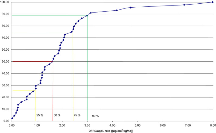
Cumulative initial DFR/Application rate
It is allowed to refine the assessment for dissipation (decay) of the active substance on the foliage if the exact nature of the dissipation over time is known. If no data are available on the degree of dissipation, it may be assumed that active substances which are organic chemicals, and for which there is evidence of breakdown, e.g. by photolysis or hydrolysis in soil or water, or decline of concentration due to plant growth will dissipate with a half‐life of 30 days. For other categories of active substance DFR0 is used in the respective calculations.
For PPPs with multiple treatments sought, the assessment should consider the potential accumulation of DFR from successive treatments. If no experimental data are available, and an active substance is assumed to dissipate with a half‐life of 30 days (this value differs from that proposed in the birds and mammals opinion (EFSA, 2008) because it was decided to follow a more conservative approach based on the available data indicating possible DT50 values up to and exceeding 30 days for some active substances), the dissipation should be taken into account by application of an appropriate multiple application factor (MAF), examples of which are given in Table 63.
Table 63.
Multiple application factors, assuming a default dissipation half‐life of 30 days (EFSA PPR Panel, 2015b; EFSA Guidance, 2014)
| Daysa | Number of applications | |||||||||||
|---|---|---|---|---|---|---|---|---|---|---|---|---|
| 1 | 2 | 3 | 4 | 5 | 6 | 7 | 8 | 9 | 10 | 11 | 12 | |
| 7 | 1.0 | 1.9 | 2.6 | 3.2 | 3.7 | 4.2 | 4.5 | 4.9 | 5.1 | 5.4 | 5.6 | 5.7 |
| 10 | 1.0 | 1.8 | 2.4 | 2.9 | 3.3 | 3.6 | 3.9 | 4.1 | 4.2 | 4.4 | 4.5 | 4.5 |
| 14 | 1.0 | 1.7 | 2.2 | 2.6 | 2.9 | 3.1 | 3.2 | 3.3 | 3.4 | 3.5 | 3.5 | 3.5 |
| 21 | 1.0 | 1.6 | 2.0 | 2.2 | 2.4 | 2.5 | 2.5 | 2.6 | 2.6 | 2.6 | 2.6 | 2.6 |
Interval between applications.
For new active substances, it will be possible to consider any new experimental data in the exposure calculator; refined calculations with specific values are not considered necessary when exposure estimates in the first tier are below the established trigger.
Transfer coefficient (TC)
The transfer of residues from the plant surface to the clothes or skin of the worker is taken into account, regardless of the product applied. The level of exposure depends on the intensity, frequency and duration of contact with the foliage. This is determined by the nature and duration of the activity during re‐entry to the treated crop. Therefore, it is possible to group various crop habitats and re‐entry activities.
| (2) |
The indicative TC values in Table 64 are based on and modified from EUROPOEM II (2002) and in consideration of US EPA values and apply to both outdoor and indoor scenarios. These values are used in first‐tier assessments of potential dermal exposure for the scenarios specified. Three sets of TC values are given, according to whether or not it can be assumed that the worker will wear clothing that covers the arms, body and legs. It is assumed that harvesting is performed with bare hands or with gloves, and that dermal exposure to the body is reduced 10‐fold by clothing covering the arms, body and legs. When no PPE and no workwear are worn, exposures may be higher than these estimates and potential exposure should be estimated using the values in the fourth column of Table 61.
Table 64.
Transfer coefficients (TCs) (modified from EUROPOEM II (2002) considering US EPA, 2012; for both outdoor and indoor scenarios)
| Crop | Nature of task | Main body parts in contact with foliage | TC (cm2/h), total potential exposure | TC (cm2/h) assuming arms, body and legs covered (workwear; bare hands) | TC (cm2/h), covered body (workwear) and gloves (PPE) | Applicable for the following crops |
|---|---|---|---|---|---|---|
| Vegetables | Reach/pick | Hand and body | 5,800 | 2,500 | 580 | Brassica vegetables, fruiting vegetables, leaf vegetables and fresh herbs, legume vegetables, bulb vegetables |
| Tree fruits | Search/reach/pick | Hand and body | 22,500 | 4,500 | 2,250 | Citrus, cane fruits, oil fruits, pome fruits, stone fruits, tree nuts |
| Grapes | Harvesting and other activities (e.g. leaf pulling and tying) | Hand and body | 30,000 | 10,100 | No justified proposal possible (data missing) | n.a. |
| Strawberries | Reach/pick | Hand and forearm | 5,800 | 3,000 | 750 | Berries and other small fruit, low |
| Ornamentals | Cut/sort/bundle/carry | Hand and body | 14,000 | 5,000 | 1,400 | Ornamentals and nursery |
| Golf course, turf or other sports lawns | Maintenance | Hand and body | 5,800 | 2,500 | 580 | n.a. |
| General | Inspection, irrigation | Hand and body |
12,500 7,500 |
1,400 | No justified proposal possible | Cereals, grassland and lawns, hops, oilseeds, root and tuber vegetables, sugar beets, etc. |
These TC values may be extrapolated to other re‐entry scenarios, where the intensity and duration of contact with the foliage is judged to be similar.
For reptiles and amphibians, the TC could be assumed to be equal to the part of the total surface area of their body in contact with soil or plants and the frequency (times of contact) with the contaminated crop.
According to the EFSA Guidance, the following points are noted:
| (3) |
SDE: systemic dermal exposure (mg a.s./kg bw per day)
DFR: dislodgeable foliar residue (μg/cm2) as 1st 3 μg/cm2) (default; EFSA, 2014)
MAF: multiple application factor ‐ EFSA Guidance (2014) – Table 60)
AR: application rate (kg a.s./ha) List of intended uses (GAP)
TC: transfer coefficient (cm2/h) EFSA Guidance (2014) – Table 61)
T: duration of exposure h/day – 2 h/day for crop inspection or irrigation activities
– 8 h/day for activities such as harvesting, cutting, sorting, etc. (defaults; EFSA, 2014)
DA: dermal absorption – the higher of the values for the product and for the in‐use dilution
BW: body weight of worker (kg 60 kg)
Dermal exposure for resident
The dermal exposure for resident can take place as a result of exposure to drift, via contact with surface deposits and entry into treated fields.
Spray drift:
The total systemic exposures from spray drift should be calculated using the following equation:
Dermal exposure × dermal absorption percentage + inhalation exposure
As presented in the respective EFSA Guidance (2014) ‘Guidance on the assessment of exposure of operators, workers, residents and bystanders in risk assessment for plant protection products’, the dermal exposures (75th percentile and mean values) for residents are as shown in Tables 65 and 66.
Table 65.
Dermal exposures for residents (75th percentile from data on potential dermal exposures) (adapted and amended from EFSA PPR Panel, 2015b)
| Method of application (distance from sprayer) | ||
|---|---|---|
| Dermal (mL spray dilution/person) | ||
| Adults | Children | |
| Arable/ground boom sprayer (from BREAM) | ||
| 2 m | 0.47 | 0.33 |
| 5 m | 0.24 | 0.22 |
| 10 m | 0.20 | 0.18 |
| Orchard/broadcast air assisted applications (Lloyd et al. 1987) a | ||
| 2–3 m | n.a. | n.a. |
| 5 m | 5.63 | 1.689 |
| 10 m | 5.63 | 1.689 |
n.a.: not available.
The only available values are for the 8‐m distance downwind from the middle of the tree trunk, which are assumed to represent a 5‐m distance from the edge of the orchard; the same value is used for 5 and 10 m.
Table 66.
Dermal exposures for residents (mean data on potential dermal exposures) (adapted and amended from EFSA PPR Panel, 2015b)
| Method of application (distance from sprayer) | ||
|---|---|---|
| Dermal (mL spray dilution/person) | ||
| Adults | Children | |
| Arable/ground boom sprayer (from BREAM) | ||
| 2 m | 0.22 | 0.18 |
| 5 m | 0.12 | 0.12 |
| 10 m | 0.11 | 0.10 |
| Orchard/broadcast air assisted applications (Lloyd et al. 1987) a | ||
| 2–3 m | n.a. | n.a. |
| 5 m | 3.68 | 1.11 |
| 10 m | 3.68 | 1.11 |
n.a.: not available.
The only available values are for the 8‐m distance downwind from the middle of the tree trunk, which are assumed to represent a 5‐m distance from the edge of the orchard; the same value is used for 5 and 10 m.
For arable crops, it was agreed that BREAM data provide a better estimate of exposure and are more representative of modern practices. The BREAM results do not provide values for upwards spraying.
For orchard crops and vines, the most appropriate data set out of the three presented is the data set for conventional nozzles (no drift reduction technologies) applying 470 L/ha from a report by Lloyd et al. (1987) for an 8‐m distance downwind from the middle of the tree trunk. This data set gave the highest drift exposures in that report and the respective values are considered to be suitable for a resident located about 5 m from the edge of a field, assuming the space from the tree trunk to the edge of the field is at least 3 m.
Surface deposits:
Dermal exposure from surface deposits based on spray drift should be based on the following equation (EFSA PPR Panel, 2015b):
| (4) |
where:
SERD = systemic exposure of residents via the dermal route (mg/kg bw per day)
AR = application rate (mg/cm2) (consider MAF, if necessary)
D = drift (%) (if multiple applications have to be taken into account, a lower percentile could be considered for risk refinement)
TTR = turf transferable residues (%) (for products applied in liquid sprays, 5%, and for products applied as granules, 1% (these values come from data obtained using the Modified Californian Roller Method (Fuller et al., 2001; Rosenheck et al., 2001) and represent the upper end of the range from a number of studies with different compounds))
TC = transfer coefficient (cm2/h) (default values of 7,300 cm2/h for adults and 2,600 cm2/h for children are recommended, TC values take into account minimal protection from clothes)
H = exposure duration (h) (a default value of 2 h is recommended by US EPA, 2001)
DA = dermal absorption (%)
BW = body weight (kg).
Values for drift percentage should be taken from Table 67, as appropriate.
Table 67.
Ground sediments based on drift as a percentage of the application rate
| Distance | Field cropsa | Fruit crops, early stagesb | Fruit crops, late stagesb | Grapesb | Hopsb | |||||
|---|---|---|---|---|---|---|---|---|---|---|
| Mean | P75 | Median | P77 | Median | P77 | Median | P77 | Median | P77 | |
| 2–3 m | 4.1 | 5.6 | 18.96 | 23.96 | 6.96 | 11.01 | 5.25 | 6.90 | 9.95 | 15.93 |
| 5 m | 1.8 | 2.3 | 11.69 | 15.79 | 3.73 | 6.04 | 2.32 | 3.07 | 5.91 | 8.57 |
| 10 m | 1.0 | 1.3 | 6.07 | 8.96 | 1.6 | 2.67 | 0.77 | 1.02 | 2.91 | 3.70 |
P75: 75th percentile; P77: 77th percentile.
From BREAM.
From Ganzelmeier/Rautmann (the 75th percentile is not published).
Based on the limited availability of data, for products applied as granules, drift from applications of granules should be assumed to be 3% for broadcast (in the EFSA calculator, 3% is considered as drift on surfaces independently of the distance) and manual applications. Further refinements could be considered based on new data. Dust drift for in‐furrow applications are considered to be negligible.
Entry into treated crops:
Entry into treated crops is based on exposure from activities such as walking in treated fields for adults.
The method used should be the same as for workers, with the same DFR and a TC based on data for inspection activities (75th percentile: 7,500 cm2/h, mean: 5,980 cm2/h), and with a 15‐min exposure. TC values are only available for adults. A factor of 0.3 has been applied to the adult TC for children re‐entering treated crops.
For entry onto treated lawns (2 h of inhalation), exposures should be calculated in the same way as surface deposits (see below as for bystander), but using a deposition percentage of 100%.
Dermal exposure of Bystander
Bystanders may be exposed briefly to plant protection products via spray drift. It is assumed that it would not take more than 5 min for the tractor to pass a bystander during which the bystander could be exposed directly.
For the estimation of bystander exposure, the same approach as for residents should be followed, except for dermal and inhalation exposure to spray drift which should be taken as 95th percentile values derived from the respective data sets. However the estimation of exposure through the four pathways should be estimated separately since they are not expected to take place at the same time.
Spray drift:
The total systemic exposures from spray drift should be calculated using the following equation:
Dermal exposure × dermal absorption percentage + inhalation exposure,
where the dermal absorption percentage is that for the in‐use dilution taken from the toxicological evaluation and dermal exposures are those shown in Table 68.
Table 68.
Dermal exposures for bystanders (95th percentile) (adapted and amended from EFSA PPR Panel, 2015b)
| Method of application (distance from sprayer) | ||
|---|---|---|
| Dermal (mL spray dilution/person) | ||
| Adults | Children | |
| Arable/ground boom sprayer (from BREAM calculator) | ||
| 2 m | 1.21 | 0.74 |
| 5 m | 0.57 | 0.48 |
| 10 m | 0.48 | 0.39 |
| Orchard/broadcast air assisted applications (Lioyd et al. 1987) a | ||
| 2–3 m | n.a. | n.a. |
| 5 m | 12.9 | 3.87 |
| 10 m | 12.9 | 3.87 |
n.a.: not available.
The only available values are for the 8‐m distance downwind from the middle of the tree trunk, which are assumed to represent a 5‐m distance from the edge of the orchard; the same value is used for 5 and 10 m.
Surface deposits:
Dermal exposures from surface deposits based on spray drift should be based on the following equation (EFSA PPR Panel, 2015b):
| (5) |
where:
SEBD = systemic exposure of bystander via the dermal route (mg/kg bw per day)
AR = application rate (mg/cm2) (consider MAF, if necessary)
D = drift (%) (if multiple applications have to be taken into account, a lower percentile could be considered for risk refinement)
TTR = turf transferable residues (%) (for products applied in liquid sprays, 5% is used, and, for products applied as granules, 1% is used. These values come from data obtained using the Modified Californian Roller Method (Fuller et al., 2001; Rosenheck et al., 2001), and represent the upper end of the range from a number of studies with different compounds
TC = transfer coefficient (cm2/h) (default values of 14,500 cm2/h for adults and 5,200 cm2/h for children are recommended; TC values take into account minimal protection from clothes)
H = exposure duration (h) (a default value of 2 h to cover resident exposure)
DA = dermal absorption (%)
BW = body weight (kg).
Values for drift percentage should be taken from Table 69, as appropriate.
Table 69.
Ground sediments as a percentage of the application rate, calculated on the basis of the 95th/90th percentile values
| Distance | Field cropsa | Fruit crops, early stagesb | Fruit crops, late stagesb | Grapesb | Hopsb |
|---|---|---|---|---|---|
| 95th percentile | 90th percentile | 90th percentile | 90th percentile | 90th percentile | |
| 2–3 m | 8.5 | 29.20 | 15.73 | 8.02 | 19.33 |
| 5 m | 3.5 | 19.89 | 8.41 | 3.62 | 11.57 |
| 10 m | 1.9 | 11.81 | 3.60 | 1.23 | 5.77 |
From BREAM, arable – ground boom.
From Ganzelmeier/Rautmann.
Drift from agricultural applications of granules (general granule application, e.g. slug pellets) is assumed to be 3% for broadcast and manual applications (‘worst case’). Dust drift for in‐furrow applications is considered to be negligible.
Entry into treated crops:
For entry into crops, the same approach as for resident should be followed.
For entry onto treated lawns, exposures should be calculated in the same way as for surface deposits (see above), but using a deposit (% of application rate) of 100%.
Conclusion on the use of human dermal exposure models
In conclusion, the equation 1, used for the first‐tier potential dermal exposure estimation for the worker could be applied for the PDE estimates of amphibians and reptiles For the application of the above approach, a number of parameters need to be assessed. More specifically, the DFR values 3 μg active substance/cm2 of foliage/kg a.s. applied/ha could be used as a first‐tier assessment. Furthermore, the TC could be estimated on the basis of the total body area of the organism(s) and its activity (contact duration with new surfaces per hour) assuming that it is in continuous contact with the treated crop for a number of hours (T). The time will depend on the behaviour of the animal and it will be estimated from the time spend in the treated crop or in the contaminated field. Furthermore, for multiple applications the MAF could be considered. If this approach will be applied the following parameters need to be identified for the most relevant life stage of the organism, in order to carry out the respective risk assessment:
The toxicological endpoint (TEP) and the respective threshold (NOAEL and acceptable level of dermal exposure) and the respective assessment factor for the conversion of the NOAEL to the toxicological threshold should also be determined in order to carry out risk assessment.
If the toxicological threshold will be derived from a study carried out via the dermal route of exposure, no dermal absorption factor is needed for risk assessment when the dermal route of exposure to be considered. In this case, the acceptable dermal exposure (Regulatory threshold for acceptable exposure = NOAELdermal/assessment factor) can be directly compared to estimated dermal exposure from the environment. However, if the toxicological threshold will be derived from oral exposure (Regulatory threshold for acceptable exposure = NOAELoral/assessment factor), information on both oral and dermal absorption is necessary (oral absorption for correction of the oral dose in order to get the systemic threshold and the dermal absorption for the estimation of the systemic dermal exposure (SDE = DE × DA) from the dermal exposure (DE) (equation 3)) to carry out risk assessment via the comparison of the respective systemic exposure levels.
In respect to information that could be retrieved from the resident and bystander dermal exposure during application as a result of spray drift, the data presented on the respective tables, are from direct measurements of simulated human exposure with different application techniques and cannot provide any information to be directly used for the estimation of amphibians and reptiles exposure.
Dermal exposure models used in bird risk assessment
Dermal exposure models from US‐EPA for birds
From Technical Description and User's Guidance Document for the Terrestrial Investigation Model (TIM) (US‐EPA, 2015). Page 50–54 of 77
The dermal exposure estimate consists of two parts:
exposure to direct intercept (= overspray of the bird – half of the body surface of the bird) and
contact to plant surfaces (dislodgeable pesticide residues on foliage)
| (6.1) |
The parameters of equation 6.1 and equations 6.2, 6.3, 6.4, 6.5, 6.6 and 6.7 are listed in Table 70 below.
Table 70.
Parameters used for equations to estimate pesticide exposure concentrations through dermal exposure. From US EPA TIM model user′s guide (https://www.epa.gov/sites/production/files/2015-06/documents/timv3_0_tech_manual.pdf)
| Symbol | Parameter Description | Variable Typea | Units |
|---|---|---|---|
| Arate | Application rate from label | Constant | lb a.i./A |
| BW | Body weight | Random | g/bird |
| Cplant(t) | Concentration of the pesticide in crop foliage at time t | Random | mg/kg |
| DAF | Dermal absorption fraction | Constant | none |
| Dcontact(t) | Incidental dermal contact dose | Random | μg pesticide/g bw |
| Ddermal(t) | Dose through dermal exposure for a pesticide at time t | Random | μg pesticide/g bw |
| Dintercept(t) | Intercepted dermal dose | Random | μg pesticide/g bw |
| DPR | Dislodgeable pesticide residues | Constant | mg/m2 |
| Fdfr | Dislodgeable foliar residue adjustment factor | Constant | Kg/m2 |
| Ffield | Fraction of on field exposure | Random | none |
| Fred | Dermal route equivalency factor | Constant | None |
| Rfoliar contact | Rate of foliar contact (6.01) | Constant | cm2 foliage/cm2 body surface (per hour) |
| SAtotal | Total surface area of bird | Random | cm2 |
| TPR | Total pesticide residues | Constant | mg/kg |
‘Constant’ indicates that the parameter is set to one value. ‘Random’ indicates that the parameter's value varies based on a distribution of possible values.
Exposure from Interception (overspray):
| (6.2) |
| (6.3) |
The application rate is multiplied by 11.2 to convert the application rate from lb a.s./A to metric units to generate a concentration value expressed in μg a.s./g bw.
Dermal exposure from contact to plant surfaces:
| (6.4) |
| (6.5) |
| (6.6) |
| (6.7) |
The dislodgeable foliar residue adjustment factor (Fdfr) is needed to convert the total residues expressed in terms of mass of pesticide per unit fresh mass of vegetation (mg a.s./mg foliage) to dislodgeable pesticide residues expressed in terms of mass of pesticide per surface area of the vegetation. It is the quotient of dislodgeable residues and total residues measured immediately after pesticide application. A default Fdfr value of 0.62 (based on mean residue value from foliage of 28 mg a.s./m2/45 mg a.s./kg) is applied if no residue data are available.
The value of 2.8 μg a.s./cm2 of foliage per kg a.s. applied/ha is 25% (0.25) of the application rate as dislodgeable residues. The applied rate in lb/acre was converted to kg/ha with a factor of 1.12 (0.25 lb/ha × 1.12 = 0.28 kg/ha = 2.8 μg a.s./cm2). The 25% of dislodgeable foliar residues of the application rate is based on the arithmetic mean of 60 measurements of 4 pesticides in 14 different crops (see Section D 6.2 of Appendix D in the USEPA, 2012 SOP for residential pesticide exposure assessment, p. 491–497). A very high variability was observed. The standard deviation of the arithmetic mean of 0.25 is 0.23. Due to the low number of pesticides measured and the high variability observed in these measurements it is recommended to use the dislodgeable foliar residues of 3 μg a.s./cm2 of foliage per kg a.s. applied/ha. It is also used in human risk assessment and approximates the 90th percentile of the underlying data set (see Appendix H decimal exposure models used in human risk assessment).
Amphibian and reptile specific formulas for the animal's surface area are needed. The dermal adsorption fraction (DAF) would need to be adjusted for amphibians and reptiles. The default value is 1 and could be used as a conservative starting point.
The total surface area of a bird is multiplied by 0.079 which corresponds to the surface of their legs as birds will mainly be exposed via their legs. For amphibians and reptiles, the full surfaces area could come in contact with foliar residues. It may be possible to refine this assumption if data from contact surface of the animal with different crop types become available, e.g. the sides of the animal are in contact with cereals and the ventral side is in contact with crops where animals can climb (e.g. orchards).
No data are available for foliar contact rate (Rfoliar contact) of birds legs. As a surrogate, values from the estimates for farm workers hands were used (11.9–5,050 cm2/h). A default factor of 6.01 cm2 foliage/cm2 body surface is used for birds. This factor would need to be adjusted for amphibians and reptiles. Such a factor could be derived from information on the speed of movement and surface area of the animal in contact with foliage during movement.
The dermal route equivalency factor (Fred) is applied to estimated dermal exposures in order to derive an estimate of the equivalent oral dose. This is needed for calculating the total overall dose (from oral and dermal uptake) and to compare to a toxicity endpoint based on oral exposure (e.g. oral acute LD50). In situations where avian dermal and oral LD50 data are available for a pesticide, Fred is calculated by dividing the oral LD50 by the dermal LD50. Since EPA does not have a data requirement for avian acute toxicity testing via the dermal route, it is expected that a chemical‐specific dermal LD50 will rarely be available. In cases where a chemical‐specific dermal LD50 value is not available, it can be generated automatically by TIM using Equation 6.7 (Appendix G, reproduced from USEPA, 2013). This equation is based on available avian dermal and oral toxicity data. Although the data set is limited to 25 chemicals (primarily organophosphate insecticides), it has the advantage of being based on avian toxicity data for both routes of exposure.
It is not expected that oral toxicity and dermal toxicity data are available for amphibians and reptiles. This constitutes a problem for adding up the exposures and comparing them to one endpoint (either dermal or oral LD50). Whether the dermal route equivalency factor for mammals or birds could be extrapolated to amphibians and reptiles is highly uncertain. Because of the specific functions of amphibian skin for gas exchange and water regulation it is expected that amphibians will be more sensitive to dermal exposure than birds or mammals.
Overall, it is concluded that the dermal exposure model from the US‐EPA for birds could provide a basis for suggesting an exposure model for amphibians and reptiles. However, it would be necessary to use amphibian and reptile specific factors such as DAF, the surface area of the animal, foliar contact rate.
Inhalation exposure
Inhalation exposure models used in human risk assessment
Inhalation exposure of worker
Worker inhalation exposure may be to vapour and/or airborne aerosols (including dust). Exposure via the inhalation route is considered to have limited contribution to the total exposure in comparison to the dermal route. Currently, the exposure of worker via the inhalation route is considered for tasks carried out indoors. The estimated exposure is depended on the Task Specific Factor which can be used in the first tier of exposure and risk assessment and the only available set of exposure data is for harvesting and re‐entry in ornamental greenhouses. Worker exposure estimates for the inhalation route after outdoor applications are only necessary in exceptional cases (e.g. for volatile substances). In this case an ad hoc approach is necessary.
Inhalation exposure of Resident
Resident inhalation exposure may take place as a result of exposure to drift or to vapour.
For the estimation of inhalation exposure via drift, the 75th percentile and the mean of exposure to spray solution for both adults and children following arable/ground boom applications as well as orchard broadcast applications are given in Tables 71 and 72.
Table 71.
Inhalation exposures for residents (75th percentile from data on potential inhalational exposures) (adapted and amended from EFSA PPR Panel, 2015b)
| Method of application (distance from sprayer) | These values are the 75th percentiles for residents (assuming average breathing rates for inhalation exposures) | |
|---|---|---|
| Inhalation (mL spray dilution/person) | ||
| Adults | Children | |
| Arable/ground boom sprayer(from BREAM) | ||
| 2 m | 0.00010 | 0.00022 |
| 5 m | 0.00009 | 0.00017 |
| 10 m | 0.00009 | 0.00013 |
| Orchard/broadcast air assisted applications (Lloyd et al. 1987) a | ||
| 2–3 m | n.a. | n.a. |
| 5 m | 0.0021 | 0.00164 |
| 10 m | 0.0021 | 0.00164 |
n.a.: not available.
The only available values are for the 8‐m distance downwind from the middle of the tree trunk, which are assumed to represent a 5‐m distance from the edge of the orchard; the same value is used for 5 and 10 m.
Table 72.
Inhalation exposures for residents (mean data on potential inhalational exposures) (adapted and amended from EFSA PPR Panel, 2015b)
| Method of application (distance from sprayer) | These values are the mean values (assuming average breathing rates for inhalation exposures) | |
|---|---|---|
| Inhalation (mL spray dilution/person) | ||
| Adults | Children | |
| Arable/ground boom sprayer (from BREAM) | ||
| 2 m | 0.00009 | 0.00017 |
| 5 m | 0.00008 | 0.00014 |
| 10 m | 0.00007 | 0.00011 |
| Orchard/broadcast air assisted applications a | ||
| 2–3 m | n.a. | n.a. |
| 5 m | 0.00170 | 0.00130 |
| 10 m | 0.00170 | 0.00130 |
n.a.: not available.
The only available values are for the 8‐m distance downwind from the middle of the tree trunk, which are assumed to represent a 5‐m distance from the edge of the orchard; the same value is used for 5 and 10 m.
Exposures to vapour should be estimated using the method that has been developed in the UK (CRD, 2008) and Germany (Martin et al., 2008), based on the highest time‐weighted average exposure for a 24‐h period, according to the volatility of the active substance:
SERI = (VC × IR × IA)/BW (equation 6), where:
SERI = systemic exposure of residents via the inhalation route (mg/kg bw per day)
VC = vapour concentration (mg/m3)
IR = inhalation rate (m3/day)
IA = inhalation absorption (%)
BW = body weight (kg)
For moderately volatile compounds (vapour pressure ≥ 0.005 Pa and < 0.01 Pa), exposures should be calculated assuming a default concentration in the air of 15 μg/m3 and daily average breathing rates, resulting in:
an adult value of 15 μg/m3 × 0.23 m3/day/kg × 60 kg = 3.45 μg/day/kg × 60 kg = 207 μg/day
For compounds with low volatility (vapour pressure < 0.005 Pa), exposures should be calculated assuming a default concentration in the air of 1 μg/m3 and the daily average breathing rates, resulting in:
an adult value of 1 μg/m3 × 0.23 m3/day/kg × 60 kg = 0.23 μg/day/kg × 60 kg = 13.8 μg/day.
Any future possibility of modifying the vapour pressure value and the concentration in the air will allow a refinement of the exposure calculations.
Inhalation exposure of Bystander
Bystander inhalation exposure may happen via exposure to spray drift or to vapour. The 95th percentile of bystander inhalation exposure via drift assuming high inhalation breathing rate both for arable/ground boom sprayers and orchard broad cast air assisted applications for adults and children are given in Table 73. The exposure to vapours should be calculated in the same way as for residents.
Table 73.
Inhalation exposures for bystanders (95th percentile) (adapted and amended from EFSA PPR Panel, 2015b)
| Method of application (distance from sprayer) | 95th percentiles for bystanders (assuming high breathing rates for inhalation exposures) | |
|---|---|---|
| Inhalation (mL spray dilution/person) | ||
| Adults | Children | |
| Arable/ground boom sprayer (from BREAM calculator) | ||
| 2 m | 0.00050 | 0.00112 |
| 5 m | 0.00048 | 0.00083 |
| 10 m | 0.00051 | 0.00076 |
| Orchard/broadcast air assisted applications ((Lloyd et al. 1987) a | ||
| 2–3 m | n.a. | n.a. |
| 5 m | 0.0044 | 0.0035 |
| 10 m | 0.0044 | 0.0035 |
n.a.: not available.
The only available values are for the 8‐m distance downwind from the middle of the tree trunk, which are assumed to represent a 5‐m distance from the edge of the orchard; the same value is used for 5 and 10 m.
Conclusion on the use of residents and bystander inhalation exposure assessment:
Inhalation exposure of both residents and bystanders may happen as a result of exposure to airborne spray during application or due to exposure to vapours. In respect to information that could be retrieved from the resident and bystander inhalation exposure during application as a result of spray liquid inhalation, the data presented in the tables above are from direct measurements of simulated human exposure with different application techniques and cannot provide any information to be directly used for the estimation of amphibians and reptiles inhalation exposure.
For the estimation of amphibian and reptile exposure due to inhalation of vapours, the principle of the approach followed for resident and bystander exposure could be applicable as well (equation 6). In this case, the vapour concentration for compounds of low volatility is assumed to be 1 μg/m3 while for moderately volatile 15 μg/m3. However, for the application of equation 6 in case of amphibians and reptiles the inhalation rates of the animals are needed.
Inhalation exposure in bird risk assessment
Inhalation exposure model for birds from US EPA
The inhalation exposure calculations and the parameters in Table 74 are from the Technical Description and User's Guidance Document for the Terrestrial Investigation Model (TIM) Page 44–50.
Table 74.
Parameters used for equations to estimate pesticide exposure concentrations through inhalation exposure. From US EPA TIM model user′s guide (https://www.epa.gov/sites/production/files/2015-06/documents/timv3_0_tech_manual.pdf)
| Symbol | Parameter Description | Variable Type* | Units |
|---|---|---|---|
| Arate | Application rate from label | Constant | Lb a.i./A |
| Bvol | The volume‐based biotransfer factor, function of Henry's law constant and log Kow | Constant | μg/L fresh weight leaf/μg/L air |
| BW | Body weight | Random | g/bird |
| Cair(drops)(t) | Pesticide concentration in a volume of air for the time step immediately following the pesticide application | Constant | μg/mL |
| Cair(t)(volume) | Concentration of the pesticide in air at time t (resulting from volatilisation); function of Mpesticide mplant and Bvol | Random | μg/mL |
| CH | Height of crop | Constant | m |
| D | Fraction of hour where pesticide is applied | Constant | None |
| Dinhalation | Dose through inhalation for a pesticide at time t | Random | μg pesticide/g‐bw |
| Dspray(t) | Droplet inhalation dose | Random | μg pesticide/g‐bw |
| Dvapor(t) | Volatilisation inhalation dose; function of pesticide concentration in air, volume of inhaled air, and body weight of the bird | Random | μg pesticide/g‐bw |
| FAM | The ratio of avian to mammalian pulmonary membrane diffusion rates from USEPA 2013 | Constant | None |
| Fre | Fraction of on field exposure | Constant | None |
| Frespired | Volumetric fraction of droplet spectrum not exceeding the upper size limit of respired particles for birds | Constant | None |
| H | Henry's law constant | Constant | atm‐m3/mol |
| IS | Inhalation scale factor | Random | None |
| Kow | Octanol–water partition coefficient | Constant | None |
| LD50 | Lethal dose sufficient to kill 50% of exposed individuals | Constant | mg/kg = μg/g |
| Mpesticide | The pesticide concentration on the treated field at time t (accounting for dissipation); function of application rate | Random | mg |
| mplant | The mass of plant (crop) per ha based on user input | Constant | kg |
| R | Universal gas constant (8.205 e−5) | Constant | atm‐m3/mol‐K |
| RH | Height of spray release | Constant | m |
| Rrate | Respiration rate | Random | mL/h |
| T | Air temperature | Constant | K |
| Vair | The volume of air in 1 ha to a height equal to the height of the crop canopy | Constant | L |
| Vinhalation | Volume of air respired | Random | mL |
| ρplant | The density of the crop tissue assumed as fresh leaf (0.77) | Constant | Kg/L |
* ‘Constant’ indicates that the parameter is set to one value. ‘Random’ indicates that the parameter's value varies based on a distribution of possible values.
As in the human inhalation exposure there is a differentiation in dose received from spray droplets Dspray(t) and from vapour Dvapor(t).
| (5.1) |
with:
Dspray(t) is the dose received from inhalation of spray droplets.
Dvapor(t) is the dose received from inhalation of vapour.
Ffield is the fraction of field exposure and is calculated by Monte Carlo simulation.
Fre is the oral dose equivalence factor which is applied to estimated inhalation exposures in order to derive an estimate of the equivalent oral dose.
Inhalation of droplets:
| (5.2) |
Fraction of applied pesticide spray (Frespired) – only droplets with a size of < 100 μm are considered to be inhaled. The default value of the fraction of spray inhaled is 0.28.
Pesticide concentration in a volume of air (C air(t)drops )):
| (5.3) |
The hight of spray release (RH) is a constant value of either 1 or 3.3 m
D = 0.025 based on 90 s duration of direct spray inhalation for ground spray applications
D = 0.0083 based on 30 s duration of direct spray applications
The factor of 0.112 is used to convert lb a.i./A to metric units and to give a concentration expressed in μg a.i./mL.
Calculation of Inhaled Air Volume (V inhalation ):
| (5.4) |
The inhalation rate is varied randomly from a beta distribution of values from 0.9 to 1.1 (mean = 1) (factor S1) to allow variation depending on the different activity levels between different hours (this is because all exposure routes are considered in a probabilistic approach).
A factor of 3 is applied to account for greater volumes inhaled in the field than in the laboratory.
Allometric equation to calculate the respiration rate:
| (5.5) |
Inhalation of vapour phase:
Two compartments are considered: crop leaf and air between crop and soil. Dissipation between the total pesticide mass applied to a 1‐ha treated field (Mpesticide; Equation 5.8) combined with dissipation between the time of application and time t are used to estimate the total mass of pesticide available for partitioning between crop leaf and canopy air. The density of the crop tissue (ρ plant) assumed to be fresh leaf is 0.77 kg/L, based on the Hazardous Waste Identification Rule (HWIR) Farm Food chain Model (USEPA, 1999). The air compartment volume (Vair) is represented by a 1‐ha area, with a height set at the top of the canopy at time of application (Equation 5.9). The available pesticide residue is then partitioned between the two compartments (air and leaf mass) through the application of the volume‐based biotransfer factor (Bvol) developed for the HWIR model (Equation 5.10). It is assumed that the air temperature (T) is a constant value of 298.1 K (equivalent to 25°C, 77 F). A temperature of 25°C was chosen because Henry's law constant and octanol–water partition coefficient (Kow) values for pesticides are frequently available at this temperature; however, the relevance to the actual environment at the time of pesticide application is an uncertainty. The total available residues establish an upper limit of available pesticide concentration in the air as a result of volatilisation from (treated) leaf surfaces.
| (5.6) |
| (5.7) |
| (5.8) |
| (5.9) |
| (5.10) |
It is concluded that the exposure estimates for birds could in principle be used for amphibians and reptiles after adjusting it with amphibian and reptile specific factors for inhaled air volumes.
Ventilation rates and oxygen consumption of different reptile groups and birds and mammals were compared in a review article by Bennett, 1973. Higher ventilation rates of homeotherms are principally the result of a greater ventilation frequency in mammals and a greater tidal volume in birds. The inhaled volume of air per minute is about 3.6 times and 4.9 times greater in birds and mammals compared to reptiles.
It is expected that the contribution of inhalation exposure to the total exposure is much less than oral and dermal exposure and therefore it is considered not necessary to assess inhalation exposure by default. However, an inhalation exposure assessment may be needed if a substance is volatile and very toxic to reptiles. Inhaled volumes in amphibians are likely to be even less than for reptiles as their skin has an important function for gas exchange. Therefore, it is not considered necessary to conduct an inhalation exposure assessment for amphibians.
Oral exposure
Herptox model of US‐EPA
Oral exposure in T‐Rex/T‐Herps models from USEPA
The oral exposure assessment procedure used by the USEPA is based on very similar principles as the SANCO EFSA Guidance documents for birds and mammals (EFSA, 2015a). The overall process is based on the estimate of residues on dietary items after application of a given plant protection product. Several models are available not only for foliar and granular application, but also for seed treatment. The Kenaga transfer coefficients, modified by Fletcher, are used to determine residual concentrations of PPPs on dietary items. Half lives of ASs (first‐order kinetics), application rate, number of application(s), interval between applications are taken into account to simulate exposure estimates for 1 year. Upper bound Kenaga results are used for risk assessment but can be refined in higher tier assessments. The T‐Rex model has been developed to fit various birds and mammal species (see Table 75). It is assumed that the mass fraction of water will be 80% for herbivores and insectivores, but only 10% for granivores. A major difference with the SANCO model lies in the species‐specific scenarios used. In the USEPA models, the species are theoretical species with either herbivorous, insectivorous or granivorous regimen, used as worst‐case scenarios in a first‐tier approach. Food intake estimates with the USEPA and SANCO models are povided in Tables 75 and 76.
Table 75.
Food intake estimates for bird and mammalian species in the T‐Rex model (USEPA)
| Species | Organism/body weight (g) | Food Intake (g/day) | Percent body weight consumed (g/day) | ||
|---|---|---|---|---|---|
| Herbivores/insectivores | Granivores | Herbivores/insectivores | Granivores | ||
| Small mammal | 15 | 14.3 | 3.2 | 95 | 21 |
| Medium mammal | 35 | 23 | 5.1 | 66 | 15 |
| Large mammal | 1,000 | 150 | 34 | 15 | 3 |
| Small bird | 20 | 23 | 5 | 114 | 25 |
| Medium bird | 100 | 65 | 14 | 65 | 14 |
| Large bird | 1,000 | 291 | 65 | 29 | 6.5 |
Table 76.
Examples of food intake rates based on SANCO document (EFSA, 2009)
| Species | Organism/body weight (g) | Food Intake (g/day) | Percent body weight consumed (g/day) | ||
|---|---|---|---|---|---|
| Herbivores/insectivores | Granivores | Herbivores/insectivores | Granivores | ||
| Small herbivorous mammal (Apodemus sylvaticus) | 21.7 | – | 3.7 | – | 17 |
| Small insectivorous mammal (Sorex araneus) | 9.7 | 5.3 | – | 55 | – |
| Large herbivorous mammal (Oryctolagus cuniculus) | 1,543 | 771 | – | 50 | – |
| Small granivorous bird (Carduelis cannabina) | 15.3 | – | 4.3 | – | 28 |
| Medium insectivorous bird (Glareola pratincola) | 75 | 23.2 | – | 31 | – |
| Large herbivorous bird (Anser anser) | 3,108 | 1,709 | – | 55 | – |
The European process uses the concept of focal species. These species are real species potentially exposed in their habitat to the PPP applied and biological data from scientific literature about their diet and habitat preferences. According to the type of crop, the feeding regimen is adjusted and food intake rate adjusted accordingly. The model also takes into account other variables like the interception rate for foliar application on all crop types. The scenarios are more detailed to fit all potential used and crop types.
T‐Herps is only used if standard risk evaluation with the T‐REX models for amphibians and reptiles exceeds the Level of Concern for acute (0.1) or chronic exposures (1).
The model has been adapted from the T‐Rex model developed by the USEPA. Currently, it has only been approved to assess exposure of terrestrial life stages of insectivorous herptiles (i.e. no herbivorous species have been considered). The model is based on the assumption that herptiles, as poikilotherm species, have a lower metabolic rate, a lower caloric intake requirement and, as a consequence, a lower Food Intake Rate (FIR). Evidence of this difference is provided by the estimated caloric requirements for free living iguanid lizards as compared with passerine birds:
Iguanids:
FMR = 0.0535 (BW)0.799
Passerine birds:
FMR = 2.123(BW)0.749
FMR: free‐living metabolic rate (kcal/day)
BW: body weight (g)
These equations indicate that the metabolic rate of birds can be 40 times higher than reptiles of similar body weight. This difference tends to decrease when body weight increases. As a consequence, using an avian food intake allometric equation instead of specific herptiles models would result in an over‐estimation for reptiles and terrestrial‐phase amphibians.
T‐Herps has been developed for the California red legged frog (CRLF). The following specific points have been included to adjust the basic model to Herptiles.
Food intake rate
The following equation was developed for an insectivorous iguanid (Nagy, 1987 cited in T‐Herps document).
FI = 0.013 (BW)0.773
FI = Food Intake (g/day)
It is assumed that terrestrial‐phase amphibians and reptiles have similar caloric requirements. At least one study was conducted (and cited in the T‐Herps literature) to compare food intake values of juvenile bull frogs (Rana catesbeiana) (Modzelewskii and Culley, 1974, cited in T‐Herps) with estimates obtained with this equation. The results indicate that juvenile bullfrog had daily FI ranging from 3% to ca 7% of their BW. Estimates ranged from 3% to 5% BW, which is considered close enough to fit the purpose.
Including small mammals and amphibians as potential dietary items.
T‐Herps (as well as T‐Rex, the standard model for bird and mammal exposure estimates) evaluates exposure from consumption of grass, plants, insects, seeds and fruits. T‐Herps includes different prey items, as it is recognised that some herpetofauna consume small mammals and amphibians. Herptile prey items are assumed to eat insects. These insects carry residues based on the Kenaga values. The prey size can be altered in the spreadsheet, to adjust for a specific prey.
For mammalian preys, two estimates of exposure are calculated by assuming that the prey item consumes either short grass or large insects.
Estimated daily exposure of small mammals is determined as in the general T‐REX model. (It is assumed that the same could be done with the European Guidelines).
The amount of pesticide (mg) consumed is determined by multiplying the weight of the prey item by the dose in the prey item (mg/kg).
The resulting exposure estimate is determined as the pesticide mass consumed (mg/bw of assessed species).
The mass of the prey item can be altered in the program. Default values are set at 35 g for mammals.
Water content of food items
Wet weight of food intake is used in the FIR equation. Water content of various potential food items is used in the models developed by the USEPA. The highest mean water content of the taxonomic group of prey item is used in dose calculation. For instance, default values of 69% for insects and 85% for amphibians are used.
Body weight of Herptiles
The spreadsheet is designed to include small, medium and large animals. The default values correspond to CRLF data. Critical review of values is recommended in order to adapt prey items to the assessed species.
Limitations and uncertainties
T‐Herps has been developed only for terrestrial herptiles exposure resulting from the consumption of terrestrial organism. No evaluation for aquatic organisms is included. If there is no evidence of bioaccumulation in aquatic organisms, this should not be a concern. If there is evidence of bioaccumulation in aquatic organisms, this should be included in the risk characterisation phase.
Metabolism, biotransformation or elimination from the prey item is not considered. T‐Herps assumes that the prey animal is consuming its daily intake of contaminated food before being consumed by the species of interest.
Bioaccumulation of contaminants in prey items is not included. As a consequence, exposure estimate is likely to be underestimated.
Residues present on the prey item (as a result of direct spray) is not being considered.
A default median value of 35 g is assumed for small mammal preys. Larger prey animals will result in lower dietary‐based RQs. It is not known if it is better to use dietary‐based or dose‐based RQs. If these RQs do not exceed the level of concern, it is suggested to use smaller prey items in the model.
T‐Herps does not include temperature influence on the food intake allometric equation, although there is evidence indicating that temperature will influence the FIR.
The allometric equation used to estimate FIR provides a constant daily value. T‐Herps; however, provides estimated potential exposures from different food items, with the underlying assumption that a given food item will constitute 100% of the daily diet on that given day.
Literature
Bennett AF, 1973. Ventilation in two species of lizards during rest and activity. Comp. Biochem. Physiol., 46A, 653‐671.CRD, 2008
CRD (The Chemical Regulation Directorate, UK), 2008. Bystander Exposure Guidance. Available online: http://www.pesticides.gov.uk/guidance/industries/pesticides/topics/pesticide-approvals/enforcement/resident-and-bystander-exposure-to-pesticides
EFSA Guidance (European Food Safety Authority), 2014. Guidance on the assessment of exposure of operators, workers, residents and bystanders in risk assessment for plant protection products. EFSA Journal 2014;12(10):3874, 55 pp. https://doi.org/10.2903/j.efsa.2014.3874
EFSA PPR Panel (EFSA Panel on Plant Protection Products and their Residues), 2008. Scientific Opinion of the Panel on Plant protection products and their residues on a request from the EFSA PRAPeR Unit on risk assessment for birds and mammals. EFSA Journal 2008; 734, 1–181.
EFSA PPR Panel (EFSA Panel on Plant Protection Products and their Residues), 2010. Scientific Opinion on Preparation of a Guidance Document on Pesticide Exposure Assessment for Workers, Operators, Bystanders and Residents. EFSA Journal 2010;8(2):1501, 65 pp. https://doi.org/10.2903/j.efsa.2010.1501. Available online: www.efsa.europa.eu
Fuller R, Klonne D, Rosenheck L, Eberhart D, Worgan J and Ross J, 2001. Modified California Roller for measuring transferable residues on treated turfgrass. Bulletin of Environmental Contamination and Toxicology, 67, 787–794.
Lloyd GA, Bell GJ, Samuels SW, Cross JV, Berry AM, 1987. Orchard sprayers: comparative operator exposure and spray drift study, Agricultural Science Service, Agricultural Development and Advisory Service, Ministry of Agriculture Fisheries and Food, UK.
Martin S, Westphal D, Erdtmann‐Vourliotis M, Dechet F, Schulze‐Rosario C, Stauber F, Wicke H and Chester G, 2008. Guidance for exposure and risk evaluation for bystanders and residents exposed to plant protection products during and after application Journal für Verbraucherschutz und Lebensmittelsicherheit, 3, 272–281.
Rosenheck L, Cowell J, Mueth M, Eberhart D, Klonne D, Norman C and Ross J, 2001. Determination of a standardized sampling technique for pesticide transferable turf residues. Bulletin of Environmental Contamination and Toxicology, 67, 780–786.
US‐EPA (US Environmental Protection Agency), 2015. Technical description and user's guidance document for the terrestrial investigation model (TIM) Version 3.0 BETA, March 25, 2015. Office of Pesticide Programs, Office of Chemical Safety and Pollution Prevention, U.S. Environmental Protection Agency, Washington, DC.
US EPA (US Environmental Protection Agency), 2001. Science Advisory Council for Exposure, policy number 12, recommended revisions to the standard operating procedures (SOPs) for residential exposure assessments. Office of Pesticide Programs, Health Effects Division, Washington, DC, USA.
Appendix I – Estimation of body burden in amphibians following exposure to pesticides via different dermal routes and sources (soil, vegetation)/activities (moving through the field & contact with soil, contact with treated crops)
1.
Given the complexity of the amphibian life cycle and the unique traits of the different amphibian species, the comparison of exposure levels through the different dermal routes and how they contribute to the total body burden is considered of importance for risk assessment purposes. In addition, the knowledge on how the different sources (soil, water, vegetation) of exposure may contribute to the body burden and the different activities of the animals is also of importance for the risk assessment. The realistic exposure estimation is directly linked to the reliability of risk assessment and it is the only way to get a better insight into the risks from the use of plant protection products and propose effective risk mitigation measures.
Note that the intention of this appendix is to compare the potential size of dermal uptake from various sources and to provide a theoretical framework for assessing the exposure of terrestrial life stages of amphibians. Further work is needed before it could be suggested for use in a regulatory framework.
The available information, although very limited, was gathered from different sources and from the open literature. Inspired by a toxicokinetic model for fish we propose below a toxicokinetic model for amphibians. In this model, passive and active dermal uptake are considered, as well as dermal uptake via contact with treated leaves:
# passive dermal uptake considers the uptake from the soil surface by diffusion of dissolved pesticide molecules from the soil‐pore water via the moist skin into the amphibian;
# active dermal uptake considers the uptake of water containing pesticides by the amphibian. A normal hydration has been described, as well as an increased rehydration after some degree of desiccation of the amphibian, and
# dermal uptake from foliage, i.e. uptake of pesticide mass by contact to a treated crop.
Amphibians may come into contact with pesticides by, e.g. (i) migration of adults to the breeding ponds, resulting in relatively short‐term exposure through contact on residues on the bare soil surface, or (ii) more prolonged stay in the field, resulting in a longer exposure through contact with soil surface and residues on plants.
The sources for dermal uptake mentioned above were derived from an investigation on moving behaviour of different amphibian species in agricultural land in northern Germany by Berger et al. (2011a). Amphibians crossed fields without vegetation rather quickly within a short period of time while if there was vegetation cover then they stayed for longer periods of time in the field. Furthermore, a high overlap of the time window was observed between pesticide‐application period and migration of amphibians to breeding ponds, leading to potential exposure of a high proportion of the population (Berger et al., 2011b).
In addition to these, sources for dermal uptake overspray has been considered. The main reason for doing this is that we want to use the resulting body concentration as a reference with respect to the other sources of dermal uptake. So, considering overspray does not imply a statement on its level of occurrence in the field.
In this appendix, we make use of a calculation example to give insight into the results of the equations. The calculation example is based upon an amphibian with a fresh body weight of 100 g, crossing a treated field of 580 m in 10 h which was the longest distance moved by common toad (from Berger et al. (2011a). The total body surface area SA of the amphibian has been calculated at 16.27 cm2 (Table 58 in Appendix G, allometric equation based upon body weight for all frogs). The amphibian is assumed to be in contact with soil‐pore water of the upper 1 mm soil. The soil‐pore water concentration in this upper mm (0–1 mm depth) has been estimated at 72.5 mg/L. This value equals 10 times the value of 7.25 mg/L, calculated by the PERSAM model (EFSA, 2017) for the peak concentration (t = 0) in the upper cm soil (zeco = 1 cm) after a 1 kg/ha application of standard substance 12 (Kom of 316 L/kg, i.e. a slightly mobile compound according to the PPDB classification) for the Central Zone of the EU. So, we estimated the concentration in the upper mm of soil‐pore water to be approximately 10 times higher than the average concentration in the soil‐pore water of the upper cm (the zeco in PERSAM). More sophisticated models, such as PEARL or PELMO, may be used to obtain improved estimates of the concentration in the soil‐pore water in the upper 1 mm of soil.
1.1.
Calculation of reference body concentration by overspray
The impact on body burden by overspray can most easily be defined as an instantaneous increase (pulse) instead of a prolonged uptake process. Assuming that the application of 1 kg/ha will land on half of the total body surface area of the amphibian, the increase in body burden (mg/kg) will be defined by:
 |
(1) |
with
ΔCB increase in body concentration, expressed per unit wet body weight (mg/kg)
EP absorption efficiency through skin for overspray (−)
AR application rate (kg/ha)
100 factor to transform kg/ha to mg/m2
§SA skin contact area, i.e. half of the total body surface area (m2)
BW wet body weight (kg)
Example calculation:
For EP equal to 1, the increase in internal concentration by overspray will be 0.81 mg/kg bw (see also Table 58, entry for All frogs, in Appendix G):
EP 1 (−)
100AR 100 (mg/m2)
§SA 0.00081 (m2)
BW 0.1 (kg)
Introduction to the model
The model describes the concentration of pesticide in the body of an amphibian while crossing an agricultural field that has been treated with pesticide shortly before. The model describes two dermal uptake mechanisms from soil (passive and active uptake), plus the dermal uptake by contact with foliar residues. The dietary uptake has been examined in Appendix G. The description below focuses on the dermal uptake routes; the elimination and metabolic transformation have not been further developed.
The main underlying assumptions of this model are:
The amphibian is in contact with the soil surface (including the soil‐pore water) and/or plants immediately after treatment, and
The uptake‐rate coefficients kS (passive dermal uptake of pesticide from soil), kW (active dermal uptake of water through skin and pelvic patch) and kF (uptake from contact with foliage) are constant with time. So, they are independent of e.g. the pesticide body concentration.
To obtain insight into the potential relevance of the uptake via soil‐pore water and via leaves, we estimated their maximal contribution to the body concentration by considering each source separately and making worst‐case assumptions for the exposure sources. Note that this implies that the underlying assumptions for uptake from soil‐pore water and via leaves may exclude each other, e.g. for uptake via soil‐pore water, the assumption is that the entire application rate falls on top of the soil (i.e. application to bare soil), while for the uptake from leaves, the implicit assumption is that part of the application rate is intercepted by the leaves. For a risk assessment, the specific situation in terms of crop cover would need to be considered to achieve realistic estimates of the amounts of substance reaching the soil surface and the amounts being intercepted by the vegetation.
With respect to passive and active dermal uptake from soil‐pore water, the specific underlying assumptions are:
There is no interception, the entire application rate falls on top of the soil.
Pesticide degradation in/on soil and volatilisation are not taken into account.
There is passive dermal uptake from the soil surface via uptake of freely dissolved pesticides out of the soil‐pore water via membrane diffusion into the amphibian; therefore, while the amphibian moves across the treated field, there is continuous contact between the soil‐pore water and the moist skin of the amphibian.
There is active dermal uptake of soil‐pore water via the skin (including the permeable pelvic patch) containing dissolved pesticides.
Both pesticide uptakes are linearly related to the pesticide concentration in the soil‐pore water. This implies that pesticides sorbed into soil organic matter are considered to be unavailable for uptake by the amphibian (but they may desorb into pore water and then be taken up).
With respect to the active dermal uptake of pesticides via intake of water, only a constant hydration rate has been taken into account. So, an increased initial uptake of water due to earlier desiccation of the amphibian has not been included in Equation 1. However a calculation example of water intake by a desiccated amphibian has been included in the text to give some insight into the order of magnitude of the uptake, compared with the uptake by a normally hydrated amphibian.
With respect to foliar residue uptake:
Pesticide degradation or wash‐off from leaves is not taken into account.
There is dermal uptake after contact with foliar residues by absorption via membrane diffusion. Analogous to the membrane diffusion‐type of uptake from soil, we assume that the amphibian is constantly in contact with treated leaves while moving through the treated field, so there is a constant ‘flow’ of foliar residues over the humid skin.
We assume, as a simplification, that this constant ‘flow’ of foliar residues is in contact with the left and right sides of the amphibian body. (Therefore, only 2* amphibian body height figures in Equation 26, thus is relevant for the uptake, and not the entire amphibian body surface area.)
A fraction equal to the ‘dislodgeable foliar residue’ used in human risk assessment is available for transfer into the amphibian skin.
Model description
A one‐compartment toxicokinetic model for the dynamics of internal concentration (mg/kg) CB can be formulated similar to the model defined for fish (Arnot and Gobas 2004; Armitage et al. 2013), replacing the gill‐uptake route with dermal uptake:
| (2) |
with rate constants for dietary uptake kD, for passive dermal uptake of pesticides from soil‐pore water kS, for water uptake through skin and permeable pelvic patch kW, for uptake from contact with foliage kF , and faecal egestion rate constant kE and with metabolic transformation rate constant kM. Dietary uptake depends on the fraction Pi of dietary (prey) item i with body concentration CD,i. Passive dermal uptake by diffusion of pesticides out of pore water and active uptake resulting from water uptake are related to the soil‐pore water concentration CS (freely available dissolved), while uptake from foliage contact depends on the pesticide mass on foliar area CF . Elimination by transformation and egestion depends on body concentration CB (Table 72).
Table 77.
Units of the uptake and elimination rate constants and the concentrations they relate to
| kD | kS, kW | kF | kE, kM |
|---|---|---|---|
| (kg prey)·(kg BW−1)/day | (L pore water)·(kg BW−1)/day | (m2 leaves)·(kg BW−1)/day | Per day |
| CD | CS | CF | CB |
| mg∙(kg BW−1) | mg∙(L pore water−1) | mg∙(m−2 leaves) | mg∙(kg BW−1) |
In the following, we will focus on the different exposure sources and uptake routes, but leaving out the dietary uptake. Two mechanisms of pesticide uptake via the dermal route depend on the concentration in the upper soil (pore) water layer and are: one with rate constant kS based on the diffusion through the dermal membrane from this layer, analogous to gill uptake in fish, and the other, with rate constant kW , based on the concept of continuous uptake of water through the skin and permeable pelvic patch. The third source of dermal exposure is from the dislodgeable foliar residue.
Note that the elimination routes in Figure 1 could be incomplete: an additional elimination route may exist for amphibians e.g. via the skin, with associated rate constant, that is analogous to the gill‐elimination rate constant k2 in fish. This k2 is ‘the rate constant (per day) for chemical elimination via the respiratory area (i.e., gills and skin)’ (Arnot and Gobas 2004; Armitage et al. 2013). In addition, the relevance of growth dilution should be considered, with a rate constant kG, equalling dBW/(BW∙dt). When focusing on a single day of exposure or several days, growth dilution however will be negligible.
For constant external concentrations, the dynamics of Equation 2 develop towards a steady‐state, obtained by setting , as
| (3) |
From steady‐state conditions, the bioconcentration factor (BCF), which excludes the dietary uptake (Arnot and Gobas, 2006), can be calculated as CB/CS or CB/CF resulting in respectively
| (4) |
| (5) |
Below, the chosen approach is to obtain worst‐case estimates of body burdens, resulting from the separate sources. Thus, the flows kSCS, kWCS and kFCF , all in mg/kg·day, are quantified separately. Dynamics in body burden via each of the three dermal uptake routes are
| (6) |
| (7) |
| (8) |
with explicit solutions
| (9) |
| (10) |
| (11) |
where t represents the exposure time (day), CB at t = 0 is assumed to be zero (no uptake of pesticides before the current exposure), rates kS, kW and kF are constants, and external concentrations CS and CF are assumed to be constant as well (no degradation, no spatial variability, etc.). The model formulations derived below can however easily be extended to incorporate dynamic concentrations that would result when accounting for, e.g. degradation of the pesticide.
Passive dermal uptake by contact to soil‐pore water
We defined kS in with CB in mg/kg and CS in mg/L, and thus kS in L/kg·day.
The underlying concept for the passive dermal uptake is slightly different from the concept for the uptake of pesticides in water passing through the gills in fish, equation (5) in Arnot and Gobas (2004). For an amphibian moving over the soil surface, there is uptake from the soil‐pore water via membrane diffusion into the amphibian, and the dermal uptake is a linear function of the body surface area in contact with soil. The concept of dermal uptake as a linear function of the body surface area thus differs from being a linear function of the water volume passing the gills in fish as done by Arnot and Gobas (2004). The uptake is described by the mass balance of Equation 12, with α a transfer coefficient for diffusion from the soil surface through the skin of the amphibian (m/day). For the parameter kS (L/kg day) this results in Equation 13. The underlying assumptions of our concept are that the diffusion is governed by a soil‐pore water concentration considered to be constant and that the transfer coefficient for diffusion is not influenced by the speed of movement of the amphibian. The soil‐pore water concentration has been assumed constant because (i) the amphibian moves across the field with such a speed that is samples continuously ‘fresh’ soil surface and (ii) depending on the compound properties, mass sorbed onto soil particles may desorb, thus maintaining the soil‐pore water concentration.
The mass balance equation for diffusion from soil‐pore water reads:
| (12) |
(in words: increase in pesticide mass in the amphibian is equal to mass transferred by diffusion from soil surface via the skin contact area into the amphibian during time period dt.)
with
BW wet body weight (kg)
§SA skin contact area, i.e. half of the total body surface area (m2)
α transfer coefficient for diffusion from soil surface into amphibian (m/day)
This gives the following expression for kS:
| (13) |
with
kS rate constant for passive dermal uptake of pesticides from soil‐pore water (L/kg·day)
1,000 conversion from m3 to L.
The body burden resulting exclusively from this uptake route will be given by:
| (14) |
Example calculation:
For α equal to a value of 0.1 m/day (see exploratory calculations below for data from Van Meter et al., 2008) and CS = 72.5 mg/L we obtain a CB of 24 mg/kg bw for the amphibian after crossing the treated field. Compared to the example calculation of amphibian overspray (CB of 0.81 mg/kg bw) this passive dermal uptake is approximately a factor of 30 greater. However, note that the values for α calculated from the Van Meter et al. (2008) experiments in Table 73 are overestimated, as they assume that all pesticide mass in the juvenile frogs originate from passive uptake, which is not true because the juvenile frogs also actively took up water. Another reason for being relatively high values is that Van Meter et al. (2008) used very small frogs (2.82 g) having a large body surface area to body volume ratio, thus representing a rather worst‐case dermal exposure.
α 0.1 (m/day)
§SA 8.1 10−4 (m2)
BW 0.1 (kg)
CS 72.5 (mg/L)
t 10/24 (day)
Experimental data:
When it is assumed that in the experiments of Van Meter et al. (2008), there is only one uptake route and no elimination occurring, BCF = CB/CS would equal kS·t, and we can obtain an estimate of kS from the measured BCF and next, obtain a rough estimate of the transfer coefficient for diffusion α, for example each of the 4 pesticides to which the Leopard frogs had been exposed. Juvenile frogs had been exposed for 8 h in 10‐gallon glass aquariums with approximately 1 cm of soil treated with realistic application rates of atrazine, triadimefon, fipronil and pendimethalin. Mean weight of Leopard frogs was 2.82 g, so using the allometric equation of Appendix G for body surface area as a function of body weight for all frogs, we obtain §SA = 1.03 cm2. The calculations in Table 78 are however very much exploratory. Note that in the experiments not only passive dermal uptake took place, but also active dermal uptake (by normal hydration plus rehydration after the 12 h of overnight dehydration in dry glass aquariums before placing the juvenile frogs in the glass aquariums with treated soil), which implies that the factor α will be overestimated in these calculations. Clearly more experimental work is needed to provide more information on the size of the transfer coefficient for diffusion from the soil surface into amphibians.
Table 78.
Calculated BCF, uptake rate constants kS and transfer coefficients α for Leopard frog and four pesticides in Van Meter et al. (2008). Soil‐pore water concentration in upper 1 cm soil is calculated from total soil concentration based upon ε = 0.30 (−), ρ = 1,200 (kg/m3), fOC = 0.08 (−) and pesticide‐specific KOC (m3/kg) with ε for fraction of soil pore volume, ρ for soil bulk density (values of ε and ρ estimated for the reported sandy clay loam soil), fOC for fraction organic carbon (value reported in Van Meter et al., 2015) and KOC for sorption coefficients based upon organic carbon content from the Footprint PPDB
| Leopard frog | ||||
|---|---|---|---|---|
| Pesticide | Atrazine | Triadimefon | Fipronil | Pendimethalin |
| KOC (m3/kg)a | 0.1 | 0.3 | 0.727 | 17.491 |
| Soil concentration (mg/kg in 1 cm upper soil) (CVanMeter) | 21.53 | 6.67 | 3.16 | 17.58 |
| CB,VanMeter body burden (mg/kg BW) | 5 | 0.2 | 0.5 | 0.3 |
| CS pore water conc. (mg/L) in pore water of upper 1 cm = (CVM/1,000) · ρ/(ε + ρ · foc · Koc) | 2.6097 | 0.2751 | 0.0541 | 0.0126 |
| CS pore water conc. (mg/L) in pore water of upper 1 mm | 26.097 | 2.751 | 0.541 | 0.126 |
| BCF = CB/CS (1mm) | 0.1916 | 0.07271 | 0.9242 | 2.388 |
| t (day) | 8/24 | 8/24 | 8/24 | 8/24 |
| kS = BCF/t (L/kg∙day) | 0.5748 | 0.2181 | 2.773 | 7.165 |
| α = (kS × BW)/(§SA × 1,000) (m/day) | 0.0157 | 0.00597 | 0.0759 | 0.196 |
Note that we based our exploratory calculations upon experimental data reported in Van Meter et al. (2008), except their reported Koc values, for which we used the values presented in the Footprint PPDB. The reason is that the values of 17,378 and 2,691,535 L/kg for fipronil and pendimethalin do not seem plausible given the values presented in the Footprint PPDB of 727 and 17,491 L/kg, respectively.
Active dermal uptake by soil‐pore water uptake
We defined kW in with CB in mg/kg and CS in mg/L, and thus kW in L/kg∙day.
The underlying concept here is that amphibians continuously and actively take up water by their skin incl. its permeable pelvic patch, while in contact with the soil‐pore water of the upper soil. The skin's ‘efficiency’ for uptake of pesticides can be described by a permeability factor EW (−):
| (15) |
with
EW permeability factor of the skin for the pesticide (−)
GW water uptake rate (L/day)
BW wet body weight (kg)
in which the water uptake rate depends on the surface contact area:
| (16) |
rW,h water‐uptake rate by hydration per unit contact surface area (L/m2 day)
§SA skin contact area, i.e. half of the total body surface area (m2)
The body burden resulting exclusively from this uptake route will be given by:
| (17) |
Example calculation – active dermal uptake by normal hydration only:
We assume a rW value of 144 L/m2 day (based upon a water uptake rate of 0.01 g/cm2 min at full hydration for Leopard frogs in figure 14 of Tracey, 1976), EW of 1 and all other values as specified earlier. The time t of 10 h refers to the time the amphibian crosses the field in our example. This results in a CB of 35 mg/kg bw. Compared with the example calculation of amphibian overspray (CB of 0.81 mg/kg bw) the resulting body burden of this uptake route is approximately two orders of magnitude higher and the same order of magnitude as the passive dermal uptake.
EW 1
BW 0.1 (kg)
§SA 8.1 10−4 (m2)
rW,h 144 (L/m2 d)
CS 72.5 (mg/L)
t 10/24 day
Desiccation
It may happen that amphibians have had a water shortage for some time and have become desiccated. For desiccated individuals, one could add the ‘water deficit’ that is (quickly) compensated for by an additional water uptake. This additional uptake results in an increase in body burden (mg/kg) of
| (18) |
with fH representing the relative dehydration (‐), e.g. fH of 0.1 would mean 10% weight reduction by desiccation. Conceptually, this uptake is conveniently integrated in the modelling framework by considering it as an instantaneous event, instead of a flow maintained over a certain period of time.
Example calculation active dermal uptake by rehydration after desiccation:
For the same example and fH equalling 0.1, the additional body burden would be 7.25 mg/kg. This is smaller than the one resulting from water uptake during 10 h under fully hydrated conditions.
Assuming an average rW,r_90 value (water uptake rate for 90% hydrated frog) of 173 L/m2 day for fh = 0.1 (i.e. 0.012 g/cm2 min at 90% hydration, Tracey, 1976), we calculated the time needed to replenish the water deficit (assuming 1 L = 1 kg water) as (fh × BW)/(rW × §SA) = (0.1 × 0.1)/(173 × 0.00081) = 0.0714 day (= 1.71 h). So, the desiccation would be removed within 2 h. Using this t, the exposure time in Eq. 17 we obtain the additional body burden by replenishment of the water deficit of the amphibian. For EW equal to 1, this results in CB = 7.25 mg/kg bw (and corresponds with the value calculated above). This is approximately a factor 10 higher than the CB of 0.81 mg/kg bw for amphibian overspray.
EW 1
BW 0.1 (kg)
§SA 8.1 10−4 (m2)
rW,r_90 173 (L/m2·day)
CS 72.5 (mg/L)
t 0.0714 day
Experiment assuming active dermal uptake (both hydration and rehydration after desiccation):
Van Meter et al. (2008) performed experiments placing desiccated juvenile frogs in aquaria with 1 cm treated soil and they measured their body burden after 10 h exposure. If we assume that all pesticide mass in the frogs results from active dermal uptake, i.e. by increased initial water uptake because of rehydration after desiccation, plus the water uptake by normal hydration thereafter, then the total body burden amounts to (adding CB(t) of Equation 17 to ΔCB of Equation 18):
| (19) |
when ignoring all elimination. With BCF = CB/CS:
| (20) |
This relationship can be used to obtain, from the experimental data of Van Meter et al. (2008) combined with the normal hydration rate rW,h of 144 L/m2 day, a first estimate of the value of EW (Table 79) under the assumption that the whole body burden results from the active dermal uptake of water.
Table 79.
The estimated BCF (see Table 2) for Leopard frog and 4 pesticides in (Van Meter et al., 2008) can be used to estimate EW. BW = 0.00282 (kg); §SA = 0.0001031 (m2); fH = 0.1 (assumed). The permeability factor EW ranges from 0.0045 (triadimefon) to 0.15 (pendimethalin)
| Leopard frog | |||||
|---|---|---|---|---|---|
| Pesticide | Atrazine | Triadimefon | Fipronil | Pendimethalin | |
|
|
0.012 | 0.0045 | 0.057 | 0.15 |
Foliar residue contact
The underlying concept is analogous to the concept of the uptake of water passing through the gills in fish (equation (5) in Arnot and Gobas, 2004), but their water volume passing through the gills has been replaced by the foliar surface area encountered per time unit. While moving though, the treated field there is uptake from contact with residues on foliage by the amphibian.
We defined kF in with CB in mg/kg and CF representing the areal concentration in mg/m2, and thus the uptake rate constant kF in m2/kg∙day.
For a moving amphibian, the uptake rate constant is derived from the amount of foliar residues encountered and ‘flowing over’ the humid skin, and absorbed via membrane diffusion:
| (24) |
with
EF chemical absorption efficiency for foliar uptake (−)
Fv relevant foliar area encountered per time unit (m2/day)
BW wet body weight (kg)
And CF, the areal concentration (mg/m2 foliage) being defined by:
| (25) |
with
CF concentration per surface area of leaves (mg/m2)
DFR dislodgeable foliar residues per kg/ha applied (mg/m2 foliage/(kg/ha))
AR application rate (kg/ha)
MAF the Multiple Application Factor as used in human risk assessment (−)
Fv can be further specified as
| (26) |
with
v movement velocity (m/day)
h height of the amphibian's skin area in contact with foliage (m)
And the body burden resulting exclusively from this uptake route will be given by:
| (27) |
Example calculation
With DFR = 3 μg/cm2 for 1 application of 1 kg/ha (the standard value used in human risk assessment, corresponding to 30% of the applied 1 kg/ha1) CF equals 30 mg/m2 leaves. Combined with an (arbitrary) value of 0.001 for the absorption efficiency EF and assuming h = 2 cm we obtain a CB of 6.96 mg/kg bw for the amphibian after crossing the treated field. This is approximately 10 times higher than the body concentration by overspray (CB of 0.81 mg/kg bw for an application of 1 kg/ha).
Note that the assumed value of 0.001 for EF is crucial in this calculation. We selected this order of magnitude (instead of a default value of 1) based upon comparison with values of absorption efficiencies at gill in fish (0.000509 for atrazine and 0.004219 for fipronil) by the BIONIC model (http://cefic-lri.org/projects/lri-eco21-arc-improving-the-performance-and-expanding-the-applicability-of-a-mechanistic-bioconcentration-model-for-ionogenic-organic-compounds-iocs-in-fish-bionic/) for water pH of 7.5 and temperature of 15°C. The BIONIC model is based on Arnot and Gobas (2004) and Armitage et al. (2013). The absorption coefficient (called EW in these models) depends on pH and chemical properties like Kow and pKa (see equation 5 in Armitage et al., 2013). For risk assessment, a realistic worst‐case estimate for EF would need to be determined, based upon further research, e.g. based upon testing a number of compounds with increasing KOC and/or KOW on a number of species and next determine a EF (possibly as a f(KOC/KOW)) covering, e.g. 90%. Note also that the standard dislodgeable foliar residues used in human risk assessment will probably overestimate the residues on leaves close to the soil surface in contact with the moving amphibians.
EF 0.001
BW 0.1 (kg)
v 1,392 (m/day)
h 0.02 (m)
CF 30 (mg/m2)
t 10/24 (day), corresponding to the 10 h needed to cross the 580‐m long‐treated field
Note that for reasons of comparison we used the same crossed distance of 580 m in 10 h; however when there is vegetation amphibians generally move shorter distances and may stay longer in the field.
Conclusion and recommendations
The calculations above demonstrate that, no source of exposure via the dermal route can a priori, be excluded from the risk assessment.
There is at present, however, insufficient information available on rate constants for passive dermal uptake of pesticides by diffusion from pore water through amphibian skin for an underpinned use of the dermal exposure model presented above. The same holds for permeability factors for active uptake of dissolved pesticides present in pore water and chemical absorption coefficients for foliar uptake. This implies that there is insufficient empirical basis to use the model presented for risk assessment in regulatory context.
There is therefore a need for experimental research8 on the dermal uptake of pesticides (passive and active dermal uptake from soil and uptake from foliar contact).
The dermal exposure model presented above should be tested with experimental data.
References
Armitage JM, Arnot JA, Wania F and Mackay D, 2013. Development and evaluation of a mechanistic bioconcentration model for ionogenic organic chemicals in fish. Environmental Toxicology and Chemistry, 32, 115–128.
Arnot JA and Gobas F, 2004. A food web bioaccumulation model for organic chemicals in aquatic ecosystems. Environmental Toxicology and Chemistry, 23, 2343–2355.
Arnot JA and Gobas FAPC, 2006. A review of bioconcentration factor (BCF) and bioaccumulation factor (BAF) assessments for organic chemicals in aquatic organisms. Environmental Reviews, 14, 257–297.
Berger G, Pfeffer H, Schütz Ch, Schönbrodt Th, Braun S and Hütz W, 2011a. Raumnutzung von Amphibien im Untersuchungsgebiet Eggersdorf. In: Berger G, Pfeffer H and Kalettka Th, (eds.). Amphibienschutz in kleingewässerreichen Ackerbaugebieten. Natur & Text, Rangersdorf, pp. 127–160.
Berger G, Pfeffer H and Schobert H, 2011b. Zeitliches Zusammentreffen von Amphibien mit Maßnahmen der Ackerbewirtschaftung während des Landaufenthaltes der Tiere. In: Berger G, Pfeffer H and Kalettka Th, (eds.). Amphibienschutz in kleingewässerreichen Ackerbaugebieten. Natur & Text, Rangersdorf, pp. 127–160.
EFSA (European Food Safety Authority), 2017. EFSA Guidance Document for predicting environmental concentrations of active substances of plant protection products and transformation products of these active substances in soil. EFSA Journal 2017;15(10):4982, 115 pp. https://doi.org/10.2903/j.efsa.2017.4982
Van Meter RJ, Glinski DA, Hong T, Cyterski M, Henderson WM and Purucker ST, 2014. Estimating terrestrial amphibian pesticide body burden through dermal exposure. Environmental Pollution, 193, 262–268.
Van Meter RJ, Glinski DA, Henderson WM, Garrison AW, Cyterski M and Purucker ST, 2015. Pesticide uptake across the amphibian dermis through soil and overspray exposures. Archives of Environmental Contamination and Toxicology, 69, 545–556.
Van Meter RJ, Glinski DA, Henderson WM and Purucker ST, 2016. Soil organic matter content effects on dermal pesticide bioconcentration in American toads (Bufo Americanus). Environmental Toxicology and Chemistry, 35, 2734–2741.
Tracy CR, 1976. A model of the dynamic exchanges of water and energy between a terrestrial amphibian and its environment. Ecological Monographs, 46, 3, 293–326.
Appendix J – Considerations for refinement options
1.
Higher tier risk assessment is required when lower tiers breach the relevant trigger values. Higher tier risk assessment should establish that under field conditions no unacceptable impact occurs after use of the plant protection product under the proposed conditions of use. The definition of ‘unacceptable impact’ is discussed extensively in Section 5.2. Before conducting any refined assessment, it is necessary to define the objectives and scope for the case under consideration. No general rules can be suggested to select an appropriate option for refined risk assessment. The following considerations should be considered and specific options are summarised in Figure 59 and in Table 80.
The degree by which the lower tier trigger values were breached. Stronger evidence is likely to be required if the triggers were breached by a large margin. This is especially true for assessment of acute risks from sprayed pesticides, as the field study analysis implies a rather strong expectation of mortality for pesticides which fail Tier 1 by more than a small margin. Removing this expectation would require correspondingly strong evidence in the higher tier assessment.
The general potential of each option to reduce the estimate of risk, and/or reduce uncertainty. Refinements of dietary exposure assessment may provide only limited benefit, but this may be sufficient if the first‐tier triggers were not breached by a large margin. Well‐designed field studies are much more effective for reducing uncertainty, but also more costly. Population modelling has the advantage of addressing long‐term repercussions directly, but this may be outweighed by uncertainty about the extra parameters that have to be estimated.
Indications from first‐tier studies, e.g. indications of rapid metabolism or rapid elimination may indicate that these would be fruitful targets for refinement if representative for natural situations.
The availability and relevance of existing data, and the cost and practicality of generating pertinent new data.
Ethical and policy preferences for minimising animal testing.
Figure 59.
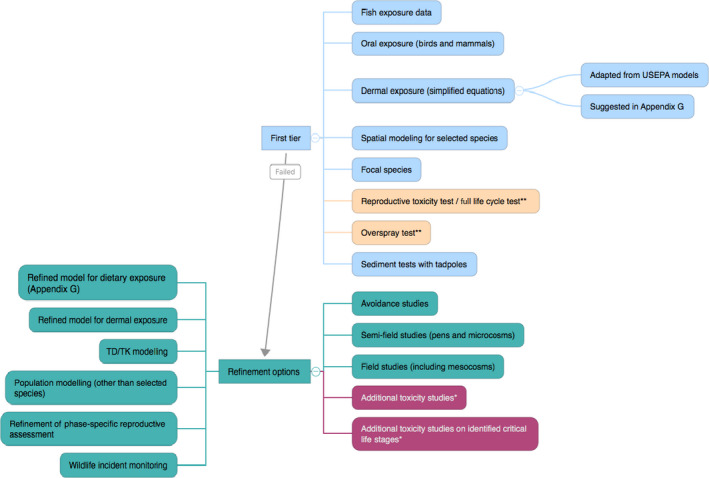
Refinement Options for Amphibians and Reptiles *not a preferred option (red) **new test (orange)
Table 80.
Overview on refinement options
| Refinement option | Possible objectives | Issues to consider |
|---|---|---|
| Refined model of exposure for dietary route | Demonstrate that effects due to dietary exposure will not exceed an unacceptable level |
|
| Refined model of non‐dietary routes of exposure | Estimate their contribution (dermal) |
|
| Specialised avoidance/repellency studies with amphibians and reptiles | Demonstrate that avoidance is sufficiently strong to ensure that lethal effects will not exceed an acceptable level |
|
| Body burden modelling | Demonstrate that the ADME characteristics of the pesticide will prevent an unacceptable level of effects |
|
| Field studies (including mesocosm studies) | Demonstrate that effects occur on acceptable proportion of occasions, or that the number of individuals and species affected is acceptable |
|
| Semi‐field studies (pen studies and microcosm studies) | Demonstrate that under realistic conditions, effects will not exceed an acceptable level |
|
| Data on wildlife incidents | Demonstrate that acute mortality occurs at least under some circumstances |
|
| Population modelling (other than selected species) | Demonstrate acceptably low risk of long‐term repercussions for abundance and diversity |
|
| Refinement of phase‐specific reproductive assessment | Demonstrate reduction in estimated risk when account is taken of relative timing of reproduction and pesticide applications |
|
| Additional toxicity studiesa | Reduce uncertainty about the distribution of toxicity between species, e.g. to justify reduction of uncertainty factors, use of geomean or SSD |
|
| Additional toxicity on the identified critical life stagea | Addresses the major concern highlighted in lower tier assessment, and generates more appropriate endpoint for that phase |
|
Not a preferred option.
Consider mesocosm studies and ponds in a field. Protection goals need to define what needs to be protected.
Since the variation in toxicity between species is one of the largest sources of uncertainty affecting risk assessment, it is a general issue that may influence the choice of refinement method. There is up to two or three orders of magnitude variation in acute LD50 between the most and least sensitive species (see Section 10.2.2). This implies up to two or three orders of magnitude uncertainty in estimating the LD50 for the focal species, and therefore up to two or three orders of uncertainty in those refinement options that involve modelling effects on a focal species (including refined TERs and body burden modelling). It also implies up to two or three orders of magnitude uncertainty in the relation between any species chosen for testing and the species actually exposed in the field. This, in turn, implies at least one or two orders of magnitude uncertainty in extrapolating from higher tier studies with captive animals (e.g. avoidance studies and pen studies) to species actually exposed in the field. It also implies up to two or three orders of magnitude uncertainty when extrapolating from a single field study site to other study sites where different species may be present. The only refinement options that avoid this problem are wildlife incident data (which underestimate risk for other reasons) and field studies with multiple sites in a sufficient diversity of conditions to encounter a representative range of species. This does not mean that field studies on multiple sites are the best option, because simpler or less costly options may be sufficient in many cases, but it does make it essential to take careful account of uncertainty about toxicity when using other options.
Amphibians and reptiles are different from birds and mammals both in terms of exposure (amphibians or reptiles may not leave a treated field as easily during pesticide application as birds or large mammals, skin permeability is different for amphibians at least, oral exposure is probably less important than dermal exposure). As a consequence, first tier options already include basic dermal absorption estimate of exposure for instance.
Appendix K – Risk management options to mitigate the risks for amphibians and reptiles
K.1. General considerations
Risk management of plant protection products (PPP) targeted at mitigating the risk for amphibians and reptiles arising from specific intended uses are at present not implemented at Member State levels. However, as a general rule, mitigation measures that are usually implemented to reduce PPP input in specific in‐ and off‐crop areas will also benefit amphibians and reptiles living in such habitats (e.g. mitigating PPP drift and run‐off into water bodies that are habitats also for tadpoles).
In‐field organisms living in or crossing fields – as it is the case, e.g. for amphibians, reptiles and birds and mammals, would profit from a general reduction of PPP input, the prohibition of very toxic products and from the provision of suitable and sufficiently large share of undisturbed habitat at landscape scale as refuge and feeding places.
Binding measures connected to the authorisation of PPPs could be the reduction of PPP input in aquatic or off‐field terrestrial habitats via drift and run‐off following the implementation of risk mitigation measures. Binding is also the application rate and number of applications, which should be reduced as far as possible without causing resistance problems.
Non‐binding measures are mostly fully voluntary and might be supported by agri‐environmental schemes. Such measures target the creation and proper management of aquatic and terrestrial habitats for amphibians and reptiles. Due to the non‐legally binding nature of such schemes, they cannot for the time being be taken into account in quantitative risk assessment procedures as measures actually reducing the degree of amphibian and reptile exposure.
General provisions and possible mitigation strategies to reduce the risk for amphibians and reptiles exposed to PPP, independent of authorisation of PPP, are listed in Table 81 and are briefly described here.
Reduced input of synthetic PPP is achieved by increasing the share of organic farming, as this practice automatically complies with the ‘greening’ obligations by the Common Agricultural Policy (CAP) and typically exceed them. Developing a taxing scheme for PPP – and in particular for those deemed to have a higher toxic impact – might also reduce their use, as it has been reported by some European States (e.g. Denmark, Sweden, and Norway see table A1, points 3a–b). Following the rules of Integrated Pest Management (IPM), as required by National Action Plans in the frame of the Pesticide Sustainable Use Directive should also reduce the use of PPP, since normally IPM and increased natural pest control substantially lowers the number of times at which PPP use is justified by economic reasons (Table 81, points 3c–d). However, these schemes with reduced PPP use may further other agricultural activities that could harm amphibians and reptiles. Therefore, a holistic approach is needed.
In order to be able to define appropriate risk mitigation for amphibians and reptiles in the future, it is indispensable to close the knowledge gaps on local and regional amphibian and reptile presence and movements and on the relationships between environmental pressures (including PPP) and population responses. For this, targeted monitoring schemes should be developed, including species but also exposure assessments. Results of monitoring schemes can be combined with already existing legally binding programs targeted at the conservation of protected and endangered species (e.g. EU Directive 92/43/EEC).
It is important to quantify the effectiveness of different mitigation strategies for the group of interest. For some strategies, there are not currently specific means of quantifying the effectiveness of these strategies. For example, the effectiveness of creating habitat corridors has a high degree of uncertainty associated with it. Amphibians may use cultivated fields when crossing field to breeding ponds (Lenhardt et al., 2013). However, it has also been reported that amphibians will strongly associate with wooded habitats near water bodies (Salazar et al. 2016) suggesting that properly hydrated corridors may in fact attract amphibians. Therefore, it is unknown to what extent an unsprayed corridor will attract amphibian species. Similarly, for reptiles it is also unknown to what extent unsprayed habitat patches are preferred habitat over cultivated fields. Two steps are necessary to quantify the effect of mitigation strategies. First, the attractiveness of the habitat needs to be quantified in relation to cultivated fields. Then, a link would be made between the SPG and the mitigation strategy (in this example, creation of habitat patches or corridors).
Table 81.
Possible management measures useful to mitigate the risk for amphibians and reptiles exposed to PPP after their intended uses in agricultural landscapes. Measures, implementation strategies, pros and cons are listed. Measures with higher probability of being implemented in the near future are highlighted in grey
| Objective | Mitigation measure | Motivation | Practical implementation | Advantages | Constraints | Chances for implementation (higher impact and probability of success are highlighted) | No. |
|---|---|---|---|---|---|---|---|
| Specific provisions to lower the exposure of amphibians and reptiles to PPP | Maintain/create higher quality habitat for amphibians and reptiles. For amphibians, this could include buffer strips around breeding ponds, wet spots and forest edges partly used as terrestrial habitat. For reptiles, this may include hedgerows, stone walls, etc. that are protected from spraying | Statutory (CAP)/personal commitment of farmers | Cross compliance for the set up and management of ecological focus areas (EFA) under CAP – minimum ecological status of EFA need to be updated. A literature review (or further research) may be needed to quantify the effectiveness of these measures | Wide application in EU; optimal management of EFA as habitat for amphibians and reptiles is likely possible | Loss of productive land possible and correspondent loss of income. Land share requested by cross compliance is min. 5%. Minimum ecological status of EFA need to be updated in order to support amphibian and reptile populations | Implemented in current CAP schemes. ‘Farmers with arable land exceeding 15 ha must ensure that at least 5% of their land is an ecological focus area with a view to safeguarding and improving biodiversity on farms. Ecological focus areas may include, for example, fallow land, landscape features, afforested areas, terraces, hedges/wooded strips or nitrogen fixing crops such as clover and alfalfa which help to improve soil organic matter. Hedges, trees, ponds, ditches, terraces, stone walls and other landscape features are important habitats for birds and other species and help protect biodiversity, including pollinators.a’ However, not all ‘greening’ measures are likely to support biodiversity and specifically amphibians and reptiles. Update of CAP after 2020 should ensure minimum quality standards for ecological focus areas | 1a |
| Voluntary | Voluntary participation supported by agro‐environmental schemes. A literature review (or further research) may be needed to quantify the effectiveness of these measures | Providing terrestrial habitats targeted to support amphibians and reptiles | Possibly participation by farmers already interested in lowering environmental impact. Low subsidies and market constraints might hamper further developments | The application of agri‐environment programmes has been compulsory for Member States in the framework of their rural development plans, whereas they remain optional for farmers. Higher financial support would increase farmers’ participation. Further improvement will depend on the CAP developments after 2020 | 1b | ||
| Convert arable land into grassland | Voluntary | Voluntary participation supported by agro‐environmental schemes | Very low or even no plant protection product application, no soil disturbance | High expenses for funding; recultivation after 5 years | The application of agri‐environment programmes has been compulsory for Member States in the framework of their rural development plans, whereas they remain optional for farmers. Higher financial support would increase farmers’ participation. Further improvement will depend on the CAP developments after 2020 | 1c | |
| Decide to waive locally the application of PPP in hot spots of amphibian and reptile presence | Voluntary | Technically possible, local support through authorities needed | No ‘loss’ of arable land | Weed infestation on fertile soils: possible lower yield with poorer quality, dedicated management with possible technical problems | Little chances of implementation due to considerable disadvantages and constraints | 1d | |
| Implement monitoring and shift time of PPP application to minimise coincidence with amphibian migration | Voluntary/provided by administration | Extensive monitoring of amphibian presence is needed to determine when PPP application timing should be altered | Less exposure of amphibians in‐field during main migration periods | Only applicable at the local scale, not translatable to other locations due to differences in amphibian phenology, time shift may benefit one population but may impact others too (‘trade‐off’), not applicable to reptiles inhabiting the field | Implementation possible; but very specific knowledge on amphibians is to be provided to farmers on site. Research and funding is needed to establish appropriate monitoring schemes. Research is needed to develop suitable models. Patchy distributed information on local presence and movements of amphibian species is already available | 1e | |
| Reduce PPP input in non‐target areas occurring via spray drift and run‐off | Statutory | Already widely implemented in PPP management (buffer strips, vegetated buffer strips and drift reducing nozzles) | Accepted risk mitigation at EU level | None | High, legally binding risk mitigation measures | 1f | |
| Measures to reduce risk of amphibians and reptiles to plant protection products by lowering toxicity | Replace PPP with expected high toxic impact by less toxic products | Voluntary | Causes higher management effort in farms, but principally applicable | Less temporal coincidence of toxic product applications with migrating amphibian populations; less toxic effects | Replacement may lead to ‘trade offs’ due to higher toxicity for other organism groups | Further scientific investigations on exposure, uptake rate and toxicity of PPP for terrestrial stages of amphibians and reptiles is required. Risk assessment scheme apt at identifying (active substances in) PPP with high toxic potential is needed. Assessment methodologies to identify alternatives for ‘candidates for substitution’ need to further developed | 2a |
| General provisions to lower the amount/discourage the use of PPP in agricultural landscape | Increase organic farming shares | Changed consumer behaviour, personal commitment of farmers, political goals | Personal commitment of farmers/supporting schemes | No synthetic plant protection products applied; sustainable land use configuration and management | There is only partly and/or temporarily awareness in European consumers with currently limited impact on conversion from conventional agricultural to organic farming | Although constantly increasing in market share, it is not expected that organic farming will be increased to a minimum quota by political will in the short range. The Rural Development Programme (2014–2020) supports the conversion to organic farming. Cross compliance under CAP is automatically achieved by organic farmers without changes of management practicesb | 3a |
| Implement additional taxes on plant protection products | Economic advantages | Toxicity of PPP to amphibians and reptiles can be incorporated into the index for taxation calculation | PPP might be used as last measure if other appropriate and less expensive cultivation measures including crop rotations fail | High uncertainty regarding the degree of implementation due to personal farmer's choices Possible unexpected market movements, less planning security for involved industrial sector | Currently, implemented in some European Member Statesc based on flat taxes, taxes on sold PPP volume or on expected environmental impact. Currently, no political signs indicating a short‐ or a medium‐term implementation in other Member States or an agreed European schemes. | 3b | |
| Apply integrated farming scheme (IF) including integrated pest management (IPM) | Currently statutory (CAP; Sustainable Use Directived) | Cross compliance | Can substantially lower the PPP input in agricultural landscapes | Initially cost and training intensive, substantial production changes might be necessary; failing in cross compliance difficult to control by administration? | Applying the principle of IPM is requested by EU policy. Increasing trend on the practical application of IPM. Medium term higher implementation to be expected | 3c | |
| Voluntary/personal commitment of farmers | Voluntary participation supported by agro‐environmental schemes | Farmers are trained and practise IPM consequently | Possibly participation by farmers already interested in lowering environmental impact. Low subsidies and market constraints might hamper further developments. | The application of agri‐environment programmes has been compulsory for Member States in the framework of their rural development plans, whereas they remain optional for farmers. Higher financial support would increase farmers’ participation. Success will depend on the CAP developments after 2020 | 3d |
CAP: Common Agricultural Policy; PPP: plant protection product; IPM: Integrated Pest Management.
PAN Europe: overview on pesticide taxation scheme in Europe https://drive.google.com/drive/folders/0BznMpGKv0fAzYkxOTUp0Z3BOOWc
Directive 2009/128/EC.
K.2. Considerations specific to amphibians
Amphibian‐focused risk mitigation strategies for PPPs have been reviewed and discussed in recent workshops and procurements (Brühl et al., 2013; Aldrich et al., 2016). For the majority of amphibian populations inhabiting agricultural lands, individuals may cross fields where PPPs are applied as part of their breeding migrations or during juvenile post‐emergence dispersal. The cases in which individuals stay for long times in fields are not very frequent (but see for instance Pelobates fuscus mentioned by Berger et al., 2013). The main goal of any mitigation strategy should be to provide high quality habitat for the organisms to use. The definition of ‘high quality’ could be variable, depending on the environment in which the crops occur. High quality would refer to uncultivated areas without direct pesticide applications and no or low PPP input from adjacent fields. For amphibians, it is necessary to establish high quality habitat in both aquatic and terrestrial environment. PPP entry into such high‐quality water bodies should be minimised. Spray drift can be reduced (Table 81, 1f) by, e.g. antidrift nozzles, buffer zones or vertical barriers such as hedges. Run‐off can be reduced by vegetated buffer strips or little dams around the ponds. Furthermore, input via drainage pipes into such habitats should be disconnected Buffer zone would also contribute to provide an upland habitat for individuals moving to and out of the water during their breeding period or during emergence. In the terrestrial environment, appropriate corridors connecting breeding and overwintering habitats should be established, provided that they are wide enough not to be sprayed or affected by drift. If no adequate overwintering habitat is located near the pond or connected by a corridor, then such habitat could be created or maintained close enough to the field to provide adequate habitat for migrating amphibians. The distance of the overwintering habitat should be determined by the species with the shortest average migration distance. In order to avoid individuals being attracted by the moisture of soil where PPPs were recently applied, it is important that habitats established as corridors keep some humidity. Areas adjacent to water courses may be used when possible, or corridors may be irrigated with clean water right after pesticides are applied to neighbour fields.
K.3. Considerations specific to reptiles
Some populations of reptiles preferentially inhabit cultivated fields (Biaggini et al. 2006, Biaggini and Corti 2015). As for amphibians, the main goal of any mitigation strategy should be to provide high quality habitat for the organisms to use, which will also refer to uncultivated areas that eliminate or reduce exposure to pesticide applications or spray drift. In the case of reptiles, however, high quality habitats would mostly be terrestrial environments. For example, uncultivated patches found throughout the habitat provide a refuge for reptiles assuming it receives no spray or minimal spray drift. In some areas, stone walls occur within fields and these would provide habitat for lizards. If these walls are unsprayed, then lizards residing within the stones will have minimal direct spray exposure. Finally, vegetated strips that are unsprayed would also qualify as higher quality habitat, again provided they are not directly sprayed or are large enough to reduce exposure to spray drift and maintain an unexposed interior. If crop rotation is used as a way of temporarily providing habitat free of PPP usage, then considerations should be made about the frequency and timing of crop rotations to minimise impacts on reptile populations that could be using the uncultivated lands for reproduction or as part of their home range. If tilling occurs too often during the growing season (e.g. more than once a season), then significant effects on reptile reproduction could happen.
Most reptile species will lay eggs, and eggs could be laid within the field. For example, grass snakes (Natrix natrix) made significant use of monoculture habitat and 25% of the time spent in monocultures occurred during the period of oviposition (Wisler et al. 2008). The previous report did not monitor egg nesting sites, but presumably the snakes could have laid eggs in the field. Madsen (1984) reported that gravid females preferred manure hills, presumably due to high humidity and temperature. Ultimately, it is currently difficult to assess risk for reptile eggs; therefore, it is also difficult to determine mitigation strategies for this stage. If the timing of egg laying were known with greater certainty, there could potentially be mitigation strategies focused on the timing of application, but this will be difficult with phenological plasticity as well as the variability of needs of application during the growing season.
References
Aldrich A, Junghans M, Aeberli C, Brühl CA, Streissl F and Schmidt BR, 2016. Amphibians and plant‐protection products: what research and action is needed? Environmental Sciences Europe, 28, 17.
Berger G, Pfeffer H and Schobert H, 2011. Zeitliches Zusammentreffen von Amphibien mit Maßnahmen der Ackerbewirtschaftung während des Landaufenthaltes der Tiere. In: Berger G, Pfeffer H and Kalettka T, (eds.). Amphibienschutz in kleingewässerreichen Ackerbaugebieten. Rangsdorf, Natur & Text. pp. 161–190.
Biaggini M and Corti C, 2015. Reptile assemblages across agricultural landscapes: where does biodiversity hide? Animal Biodiversity and Conservation, 38, 163–174.
Biaggini M, Dapporto L, Paggetti E and Corti C, 2006. Distribution of lacertid lizards in a Tuscan agro‐ecosystem (Central Italy). In: Corti C, Lo Cascio P and Biaggini M (eds.). Mainland and insular lacertid lizards: a Mediterranean perspective. Firenze University Press, Florence, Italy, pp. 13–21.
Bruhl CA, Alscher A, Hahn M, Berger G, Bethwell C, Graef S, Schmidt T and Weber B, 2015. Protection of biodiversity in the risk assessment and risk management of pesticides (plant protection products & biocides) with a focus on arthropods, soil organisms and amphibians. Federal Environment Agency, Dessau, Germany.
Lenhardt P, Brühl CA and Berger G, 2015. Temporal coincidence of amphibian migration and pesticide applications on arable fields in spring. Basic and Applied Ecology, 16, 54–63.
Madsen T, 1984. Movement, home range size, and habitat use of radio‐tracked grass snakes (Natrix natrix) in southern Sweden. Copeia, 1984, 707–713.
Salazar RD, Montgomery RA, Thresher SE and Macdonald DW, 2016. Mapping the relative probability of common toad occurrence in terrestrial lowland farm habitat in the United Kingdom. PLoS One, 11, e0148269.
Wisler C, Hofer U and Arlettaz R, 2008. Snakes and monocultures: habitat selection and movements of female grass snakes (Natrix natrix L.) in an agricultural landscape. Journal of Herpetology, 42, 337–346.
Appendix L – What additional information is needed for development of a guidance document?
Exposure assessment
In Section 9, Exposure Assessment Goals (EAGs) have been operationalised for the specific protection goals (SPGs) of no mortality (individuals) and population persistence (populations) for amphibians in their aquatic and terrestrial environment and reptiles in their terrestrial environment. In designing the EAGs, the WG made choices concerning the exposure pathways considered most important. Table 82 presents an overview of the selected combinations of SPG and locations for which the EAGs have been defined, including their Ecotoxicologically Relevant Exposure Quantities (EREQs).
Table 82.
Overview of selected combinations of SPG and locations for which the EAGs have been defined
| SPG | Location | |
|---|---|---|
| Amphibians | ||
| Aquatic water | Individual/no mortality | In‐field + edge‐of‐field |
| Water | Population/persistence | In‐field + edge‐of‐field |
| Sediment | Population/persistence | In‐field + edge‐of‐field |
| Terrestrial | Individual/no mortality | In‐crop |
| Off‐crop | ||
| Reptiles | ||
| Terrestrial | Individual/no mortality | In‐crop |
| Off‐crop | ||
| Population/persistence | Eggs in nests in‐crop | |
For the assessment of the SPG at individual level, the EREQ needs to be consistent with the selected ecotoxicological endpoint, and a corresponding spatial unit (SU) and a spatio‐temporal distributed statistical population of EREQ values in the SU needs to be defined, from which a desired percentile can be selected. Next, this EREQ value needs to be used in the risk assessment method.
Note that the internal body burden of the individual amphibian or reptile is a crucial concept, because this allows risk assessors to combine the various exposure routes and exposure times at the individual level. Ultimately, this is the only feasible way of assessing the ecotoxicological effect of multiple exposure routes and times in an improved, realistic way.
The missing information is specified below for models intending to evaluate the SPG of survival, i.e. SPGs at individual level and population persistence, i.e. at population level.
Missing information needed to define the EAGs in the aquatic environment for amphibians
Distribution of small surface waters hosting amphibians across the EU, (or a selection of these, representing the EU in a fit‐for‐purpose way); possibly the surface water population needs to be subdivided into, e.g. ponds, temporary water bodies, slow‐ and fast‐moving watercourses.
Spatially distributed exposure model for small surface waters, including shallow, temporary water bodies located in‐field or edge‐of‐field, simulating the internal body burden of an individual amphibian of a selected focal species by contact exposure (i.e. by spray drift, runoff, drainage entering the water) and oral exposure if relevant for the selected focal species, for all relevant water bodies across the EU and series of tens of years. When exposure via sediment is important, oral exposure (by sediment, periphyton, other food items and water) may dominate the exposure via the water layer (Tables 23–28). (Note that for substances with high Koc values, species and life stages, such as larvae, food intake via sediment or other components of the diet may be substantial.)
Missing information to define the EAGs in the terrestrial environment for amphibians
Distribution of fields with cultivated crops, which may host amphibians across the EU.
Spatially distributed exposure model simulating the internal body burden of an individual amphibian of a selected focal species by dermal exposure (i.e. by overspray, residues on soil and plants and in puddles on field) and oral exposure (i.e. in food, generally small arthropods), for all relevant cropped fields across the EU and series of tens of years (Tables 29 and 30). A comparable model is needed for the off‐crop exposure but the overspray route is replaced by the spray‐drift deposition route (Tables 31 and 32). This model will need information on amphibian behaviour, such as time amphibians spend in cropped fields and next to cropped fields, speed of movement, migration distances, percentage of individuals in a population that can be found in the field. In addition, to be able to build an operational exposure model, a focal species needs to have been selected first.
Missing information to define the EAGs in the terrestrial environment for reptiles
Distribution of fields with cultivated crops, which may host reptiles across the EU.
Spatially distributed exposure model simulating the internal body burden of an individual reptile of a selected focal species by dermal exposure (i.e. by overspray, residues on soil, plants and in puddles on the field) and oral exposure (i.e. by food, including secondary exposure via prey, water and ingested soil) for all relevant cropped fields across the EU and series of tens of years (Tables 33 and 34). Virtually the same spatially distributed model may be suitable for reptile eggs in nests in‐crop, if only contact exposure via residues in soil is considered and all other exposure routes set to zero (Tables 37 and 38). A model comparable to the in‐crop model is needed for the off‐crop exposure but spray‐drift deposition would replace the overspray route (Tables 35 and 36). This model will need information on reptile behaviour, such as time reptiles spend in cropped fields and next to cropped fields, burial behaviour, amount of food ingested in one meal and time to next meal, percentage of individuals in a population that can be found in the field. In addition, to be able to build an operational exposure model, a focal species need to have been selected first.
Effects assessment
There is generally a shortage of sufficient data on effects of PPPs on amphibians and reptiles for the risk assessments. This is especially true for reptiles and for the terrestrial stages of amphibians.
The options at present are:
-
either: Use fish, birds and mammals data with assessment factors sufficiently large to take into account uncertainties about extrapolation.
-
1
— The EFSA supporting publication (Ortiz‐Santaliestra et al., 2010) suggests a high level of uncertainty in extrapolating from birds to reptiles in particular.
-
2
— Assessment factors may therefore need to be large (> 100 or > 1,000) to provide protection.
-
3
— Assessment factors should be adjusted as more information becomes available.
-
1
or: Ask for data from a minimum number of carefully designed animal tests on reptiles and amphibians.
or: Implement a verified approach for read across from endpoints with other groups of organisms and PPP with a similar mode of action.
or: Accept that SPGs are not met because these organisms, and the ecosystem services they provided, are not protected.
Prior to defining an assessment factor for amphibian and reptiles based on surrogate species, further data are required with regard to:
Interstage comparisons of sensitivity in terrestrial amphibians and in reptiles.
Field studies generating data for calculation of extrapolation factors, both for amphibians (aquatic and terrestrial) and for reptiles, covering also indirect effects due to other stressors.
Toxicity data for reptiles and terrestrial amphibians on a larger diversity of substances, matching those existing for birds and mammals and thus allowing a more robust comparison among taxa and the proper identification of potential correlations supporting the use of birds and mammals as surrogates.
Toxicity data for indigenous aquatic amphibian species to establish their relationship in sensitivity to Xenopus laevis, the most frequently tested species so far.
Toxicity data on hatchlings to make sure that fish are valid surrogates by comparing their sensitivity with that of the amphibian most sensitive life stage.
Toxicity data considering exposure routes different from waterborne pollutants that are relevant for larvae, including food and sediment ingestion, to complete exposure assessment in the aquatic environment.
Reproductive toxicity data in amphibians and reptiles from studies addressing the most sensitive endpoints and chronic exposure during critical windows in the reproductive cycle. The data need to be comparable to the reproductive toxicity data obtained in potential surrogate species (fish, birds, mammals).
Here, we suggest some tests that might be developed in order to reduce uncertainty:
-
Reproduction test with amphibians (adult exposure or/and a full life cycle).
-
1
— Determining the internal doses would help for the extrapolation from the endpoints determined in aquatic environments to terrestrial stages.
-
2
— Could also be used to assess the risk from oral exposure.
-
1
-
In order to develop an amphibian life cycle test, further research is needed with regard to:
-
1
— Test species husbandry. Xenopus tropicalis, which reaches sexual maturity in 4–6 months (compared to around 12 months for Xenopus laevis), is a candidate test species for a life cycle test. There is a need for development of husbandry guidelines of Xenopus tropicalis larvae in order to evaluate whether it is a robust enough test species to qualify in a standard OECD test.
-
2
— Endpoints. Endpoints for reproductive competence need to be further developed to optimise their sensitivity. Early life biomarkers predictive of subsequent reproductive toxicity would be useful in life cycle tests. The relationship between such biomarkers and subsequent reproductive toxicity needs to be determined.
-
1
-
Overspray test with amphibians to investigate specific local effects on amphibian skin.
-
1
— Effects on amphibian skin as respiratory and ion exchange organ need to be evaluated, since this exposure routes is not covered by other test.
-
2
— Currently, we do not have any suggestion other than an overspray test performed with/without contaminating the substrate.
-
1
-
Further research is needed on how to extrapolate the endpoints from an extended life cycle test based on LAGDA to other exposure routes and other time scales of (chronic) exposure.
-
1
— How to extrapolate from the extended life cycle test based on LAGDA to terrestrial dermal exposure routes for adult amphibians living outside the aquatic environment.
-
2
— How to extrapolate from the extended life cycle test based on LAGDA to terrestrial oral exposure routes for adult amphibians living outside the aquatic environment.
-
3
— How to extrapolate from the extended life cycle test based on LAGDA to longer exposure time of adult amphibians living outside the aquatic environment.
-
4
— Extrapolation would avoid additional testing.
-
1
-
Sediment test with tadpoles to assess the oral uptake via sediment
-
1
— The relevance of uptake via spiked sediment compared with spiked water needs to be established.
-
2
— Comparability of the sensitivity of tadpoles exposed to sediment to studies with Chironomus riparius and Lumbriculus spp. in order to address the coverage of the current risk assessment.
-
1
-
Laboratory toxicity tests for reptiles:
-
1
— Acute effects (mortality from dermal exposure and also oral exposure).
Could adapt standard methods for birds and replace reptiles as species (e.g., OECD 223)
Dosing methods for oral exposure in lizards are already well established in the primary literature (e.g. Suski et al., 2003; Salice et al., 2012; Weir et al., 2016c)
An amphibian overspray test may also be protective of reptiles, but this would need further investigation.
-
2
— Chronic effects (reproduction, development, growth).
Could adapt standard methods for birds and replace reptiles as species (e.g. OECD 206)
These tests could be adapted for any endpoint of interest (e.g. growth) rather than focusing strictly on reproduction or other traditional chronic endpoints.
Currently, no study is available to cover egg exposures in fields; it is possible that such exposures occur, but it is not currently known to what extent these exposures are significant for risk assessment.
-
3
— It is not possible to extrapolate toxicity endpoints from birds and mammals without these data.
-
4
— A model species must be established if laboratory toxicity testing for reptiles is necessary.
Much research has been done for Sceloporus occidentalis; this is likely to be the best model species to begin with, as it requires the least work to establish a colony and the best population for culturing is already known (see Talent et al., 2002).
A European‐specific lizard model could also be developed (e.g. Lacerta or Podarcis).
-
1
Exposure and effects: 1. focal species
-
The list of focal species could be modified when more information becomes available on traits that are relevant for determining risk to amphibian and reptile species.
-
1
— The selection suggested in the Opinion is based on the currently available information.
-
2
— We only have this information for a few traits/species at present.
-
1
Further evaluation is needed of how representative are the focal species of other species in agricultural areas.
Exposure and effects: 2. development of landscape mode
Existing and new landscape models need to be developed linking exposure and effects using the ecotoxicologically relevant exposure quantities concept (EREQ). The models should follow the EFSA Opinion on Good Modelling Practice and require the following:
-
* Development of landscape simulations for member states, at a minimum for each regulatory zone, will need access to or create:
-
1
— CAP subsidy data.
-
2
— livestock data.
-
3
— management practices for all crops.
-
4
— GIS coverage and classification for non‐rotational crop area.
-
5
— farm classification and subsequent crop‐rotation model.
-
1
Exposure modelling for aquatic stages of amphibians in water bodies should be developed
-
Development of current model of great crested newt
-
1
— Pond suitability model
-
2
— Implement maternal transfer and aquatic stages toxic responses
-
3
— Exposure routes linking environmental concentration to the body burden of pesticide in the newt need to be defined and included.
-
4
— The result of exposure needs to be carefully considered since exposure may be a daily or regular occurrence in the lifetime of a newt and the combining of probabilities mathematically may over‐ or underestimate effects.
-
5
— Documentation of new and improved elements in the model.
-
1
-
Other five focal species models to be developed:
-
1
— Data collection and collation on ecology and behaviour.
-
2
— Formal model development.
-
3
— Computer model development.
-
4
— Iterative evaluation and testing.
-
5
— Sensitivity and Uncertainty Analysis.
-
6
— Documentation.
-
1
-
*Scenario development for all EU zones for all potential agricultural systems
-
1
— develop the range of GAPs that are possible to test in the model.
-
2
— select the landscapes for modelling (could be overcome in future when the whole of Europe could eventually be modelled), this includes identifying the agricultural landscapes).
-
3
— definition of the baselines (without pesticide impacts, but this could be changed), definition of baseline – simulation without the product, could be changed to simulation with other products and replacing one of the products with a new one. For active substance approval, the baseline would be without other pesticides while for product registration at member‐state level it may be beneficial to evaluate the whole treatment regime to see if the replacement of one of the products by another one will change the risk for the environment.
-
1
*Implementation of toxicity effects as standard inputs to the model system using a flexible user interface capable of representing the range of input possibilities needed.
*Implementation of flexible use (GAP) as standard inputs to the model system.
*Generation of a user interface for input and output of model system.
Prerunning all screening scenarios for Tier 1 testing.
*these are common to non‐target arthropods, in soil organisms, and probably birds and mammals – hence there is potential for efficient use of shared resources.
References
Ortiz‐Santaliestra ME, Maia JP, Egea‐Serrano A, Brühl CA and Lopes I, 2017. Biological relevance of the magnitude of effects (considering mortality, sub‐lethal and reproductive effects) observed in studies with amphibians and reptiles in view of population level impacts on amphibians and reptiles. EFSA Supporting publication 2017: EN‐1251, 151 pp. https://doi.org/10.2903/sp.efsa.2017.EN-1251
Suggested citation: EFSA PPR Panel (EFSA Panel on Plant Protection Products and their Residues) , Ockleford C, Adriaanse P, Berny P, Brock T, Duquesne S, Grilli S, Hernandez‐Jerez AF, Bennekou SH, Klein M, Kuhl T, Laskowski R, Machera K, Pelkonen O, Pieper S, Stemmer M, Sundh I, Teodorovic I, Tiktak A, Topping CJ, Wolterink G, Aldrich A, Berg C, Ortiz‐Santaliestra M, Weir S, Streissl F and Smith RH, 2018. Scientific Opinion on the state of the science on pesticide risk assessment for amphibians and reptiles. EFSA Journal 2018;16(2):5125, 301 pp. 10.2903/j.efsa.2018.5125
Requestor: EFSA
Question number: EFSA‐Q‐2011‐00985
Panel members: Paulien Adriaanse, Philippe Berny, Theodorus Brock, Sabine Duquesne, Sandro Grilli, Antonio F Hernandez‐Jerez, Susanne Hougaard, Michael Klein, Thomas Kuhl, Ryszard Laskowski, Kyriaki Machera, Colin Ockleford, Olavi Pelkonen, Silvia Pieper, Robert Smith, Michael Stemmer, Ingvar Sundh, Ivana Teodorovic, Aaldrik Tiktak, Chris J Topping and Gerrit Wolterink.
Acknowledgements: The Panel wishes to thank the members of the Working Group on amphibian and reptile risk assessment: Paulien Adriaanse, Annette Aldrich, Cecilia Berg, Philippe Berny, Kyriaki Machera, Manuel Santaliestra Ortiz, Silvia Pieper, Robert H Smith, Chris J. Topping, Scott Weir, and the hearing experts: Carsten Brühl, Peter Dohmen, US‐EPA colleagues: Brian Anderson, Catherine Aubee, Amy Blankenship, Kristina Garber, Edward Odenkirchen, Melissa Panger, Thomas Steeger, our short‐term study visitor Lara Petschick and EFSA staff member: Franz Streissl for the support provided to this scientific output.
Adopted: 22 November 2017
Reproduction of the images listed below is prohibited and permission must be sought directly from the copyright holder:
Figure 1: © Stockphoto; Figure 5: © WHO
This publication is linked to the following EFSA Supporting Publications article: http://onlinelibrary.wiley.com/doi/10.2903/sp.efsa.2018.EN-1357/full
Notes
Council Directive 91/414/EEC concerning the placing of plant protection products on the market OJ L 230, 19.8.1991, pp. 1–32.
Regulation (EC) No 1107/2009 of the European Parliament and of the council of 21 October 2009 concerning the placing of plant protection products on the market and repealing Council Directives 79/117/EEC and 91/414/EEC. OJ L 309/1, 24.11.2009, pp. 1–50.
Directive 2000/60/EC of the European Parliament and of the Council of 23 October 2000 establishing a framework for Community action in the field of water policy. OJ L 327/1, 22.12.2000, pp. 1–72.
Council Directive 92/43/EEC of 21 May 1992 on the conservation of natural habitats and of wild fauna and flora. Official Journalof the European Union L 206, p. 7–50.
Commission Regulation (EU) No 283/2013 of 1 March 2013 setting out the data requirements for active substances, in accordance with the Regulation (EC) No 1107/2009 of the European Parliament and of the Council concerning the placing of plant protection products on the market. OJ L 93, 3.4.2013, p. 1–84.
Commission Regulation (EU) No 284/2013 of 1 March 2013 setting out the data requirements for plant protection products, in accordance with the Regulation (EC) No 1107/2009 of the European Parliament and of the Council concerning the placing of plant protection products on the market. OJ L 93, 3.4.2013, p. 85–152.
Post‐application exposure of workers to pesticides in agriculture, Europoem II Project, FAIR3‐CT96‐1406, 2002.
The only publications found that were relevant (i.e. with measured body burdens) were Van Meter et al. (2014, 2015, 2016).
References
- Adkins‐Regan E, 1987. Hormones and sexual differentiation. In: Norris DO and Jones RE (eds.). Hormones and Reproduction in Fishes, Amphibians, and Reptiles. Plenum, New York. pp. 1–29. [Google Scholar]
- Adriaanse PI, Crum SJH, Elbers JA, Massop HThL and Beltman WHJ, 2015. Sediment properties in five Dutch watercourses. Indicative measurements for the registration procedure of plant protection products in The Netherlands. Alterra report 2574, 93 pp. Wageningen, The Netherlands.
- Aldrich AP, 2009. Empfindlichkeit von Amphibien gegenüber Pflanzenschutzmitteln. AGRARForschung, 16, 466–471. [Google Scholar]
- Aldrich A, Junghans M, Aeberli C, Brühl CA, Streissl F and Schmidt BR, 2015. Amphibians and plant‐protection products: what research and action is needed? Environmental Sciences Europe, 28, 17. 10.1186/s12302-016-0085-6 [DOI] [PMC free article] [PubMed] [Google Scholar]
- Alexander GJ, Hanrahan SA and Mitchell D, 2012. Assimilation efficiency and gut passage time in an African elapid snake, Hemachatus haemachatus . African Journal of Herpetology, 61, 3–13. [Google Scholar]
- Alford RS, 2010. Declines and the global status of amphibians. In: Sparling DW, Linder G, Bishop CA and Krest S (eds.). Ecotoxicology of Amphibians and Reptiles, 2nd Edition. SETAC Press, Pensacola (FL), pp. 13–45. [Google Scholar]
- Alix A, Brown C, Capri E, Goerlitz G, Golla B, Knauer K, Laabs V, Mackay N, Marchis A, Poulsen V, Alonso Prados E, Reinert W and Streloke M, 2017. Mitigating the Risks of Plant Protection Products in the Environment: MAgPIE. SETAC Press, Pensacola, FL. [Google Scholar]
- Al‐Mukhtar KA and Webb AC, 1971. An ultrastructural study of primordial germ cells, oogonia and early oocytes in Xenopus laevis. Journal of Embryology and Experimental Morphology, 26, 195–217. [PubMed] [Google Scholar]
- Altenburger R, Arrhenius A, Backhaus T, Coors A, Faust M and Zitzkat D, 2012. Ecotoxicological combined effects from chemical mixtures—Part 1: relevance and adequate consideration in environmental risk assessment of plant protection products and biocides Project No. 3709 65 404. Umweltbundesamt, Germany. Available online: (http://www.umweltbundesamt.de/publikationen/ecotoxicological-combined-effects-from-chemical).
- Altig R, 2007. A primer for the morphology of anuran tadpoles. Herpetological Conservation and Biology, 2, 71–74. [Google Scholar]
- Altig R, Whiles MR and Taylor CL, 2007. What do tadpoles really eat? Assessing the trophic status of an understudied and imperiled group of consumers in freshwater habitats. Freshwater Biology, 52, 386–395. [Google Scholar]
- Alza CM, Donnelly MA and Whitfield SM, 2016. Additive effects of mean temperature, temperature variability, and chlorothalonil to red‐eyed treefrog (Agalychnis callidryas)larvae. Environmental Toxicology and Chemistry, 35, 2998–3004. 10.1002/etc.3484 [DOI] [PubMed] [Google Scholar]
- Amaral MJ, Bicho RC, Carretero MA, Sanchez‐Hernandez JC, Faustino AMR, Soares AMVM and Mann RM, 2012a. The use of a lacertid lizard as a model for reptile ecotoxicology studies: part 2‐biomarkers of exposure and toxicity among pesticide exposed lizards. Chemosphere, 87, 765–774. [DOI] [PubMed] [Google Scholar]
- Amaral MJ, Carretero MA, Bicho RC, Soares AMVM and Mann RM, 2012b. The use of a lacertid lizard as a model for reptile ecotoxicology studies ‐ part 1 Field demographics and morphology. Chemosphere, 87, 757–764. [DOI] [PubMed] [Google Scholar]
- Amaral MJ, Sanchez‐Hernandez JC, Bicho RC, Carretero MA, Valente R, Faustino AMR, Soares AMVM and Mann RM, 2012c. Biomarkers of exposure and effect in a lacertid lizard (Podarcis bocagei Seoane) exposed to chlorpyrifos. Environmental Toxicology and Chemistry, 31, 2345–2353. [DOI] [PubMed] [Google Scholar]
- Amaral MJ, Bicho RC, Carretero MA, Sanchez‐Hernandez JC, Faustino AMR, Soares AMVM and Mann RM, 2012d. The usefulness of mesocosms for ecotoxicity testing with lacertid lizards. Acta Herpetologica, 7, 263–280. [Google Scholar]
- AmphibiaWeb , 2016. Information on amphibian biology and conservation. AmphibiaWeb, Berkeley, California. Available online: http://amphibiaweb.org/ [Accessed: September 26, 2016]. [Google Scholar]
- Andrews RM, 1976. Growth rate in island and mainland anoline lizards. Copeia, 1976, 477–482. [Google Scholar]
- Andrews RM, 1982. Patterns of growth in reptiles. In: Gans CD and Pugh FH (eds.). Biology of the Reptilia, Vol 13: Physiology D Physiological Ecology. Academic Press, London. pp. 273–320. [Google Scholar]
- Arribas R, Díaz‐Paniagua C and Gomez‐Mestre I, 2014. Ecological consequences of amphibian larvae and their native and alien predators on the community structure of temporary ponds. Freshwater Biology, 59, 1996–2008. [Google Scholar]
- Arts Gertie, Boesten Jos, Brock Theo, Deneer John and Roessink Ivo, 2015. An overview of protection goals and current and proposed guidance on environmental risk assessment procedures for non‐target plants, non‐target arthropods and bees. December 2015. Internal document Alterra, Wageningen University and Research. p. 39. [Google Scholar]
- Ashauer RI, O'Connor I, Hintermeister A and Escher BI, 2015. Death dilemma and organism recovery in ecotoxicology. Environmental Science and Technology, 49, 10136–10146. 10.1021/acs.est.5b03079 [DOI] [PubMed] [Google Scholar]
- Ashauer R, O'Connor I and Escher BI, 2017. Toxic mixtures in time – the sequence makes the poison. Environmental Toxicology and Chemistry, 51, 3084–3092. 10.1021/acs.est.6b06163 [DOI] [PubMed] [Google Scholar]
- Ashton KG and Feldman CR, 2003. Bergmann's rule in nonavian reptiles: turtles follow it, lizards and snakes reverse it. Evolution, 57, 1151–1163. [DOI] [PubMed] [Google Scholar]
- ASTM E1439 – 12 . Standard Guide for Conducting the Frog Embryo Teratogenesis Assay – Xenopus (FETAX). Active Standard ASTM E1439. Developed by Subcommittee: E50.47. Book of Standards Volume 11.06.
- ASTM E2591‐07 , 2013. Standard Guide for Conducting Whole Sediment Toxicity Tests with Amphibians. Active Standard ASTM E2591.
- ASTM E729 ‐ 96 , 2014. Standard Guide for Conducting Acute Toxicity Tests on Test Materials with Fishes, Macroinvertebrates, and Amphibians. Active Standard ASTM E729.
- Aubee CB and Glaberman S, unpublished data. Learning shift the curve: are amphibians more sensitive than their risk assessment surrogates? U.S. EPA.
- Avery RA, 1971. Estimates of food consumption by the lizard Lacerta vivipara Jacquin. Journal of Animal Ecology, 40, 351–365. [Google Scholar]
- Avery RA, 1975. Clutch size and reproductive effort in the lizard Lacerta vivipara Jacquin. Oecologia, 19, 165–170. [DOI] [PubMed] [Google Scholar]
- Baier F, Gruber E, Hein T, Bondar‐Kunze E, Ivanković M, Mentler A, Brühl CA, Spangl B and Zaller JG, 2016. Non‐target effects of a glyphosate‐based herbicide on Common toad larvae (Bufo bufo, Amphibia) and associated algae are altered by temperature. PeerJ, 4, e2641‐23. 10.7717/peerj.2641 [DOI] [PMC free article] [PubMed] [Google Scholar]
- Bakker F, 2016. Design and analysis of field studies with bees: a critical review of the draft EFSA guidance. Integrated Environmental Assessment and Management, 12, 422–428. 10.1002/ieam.1716 [DOI] [PubMed] [Google Scholar]
- Bantle JA, Fort DJ, Rayburn JR, DeYoung DJ and Bush SJ, 1990. Further validation of FETAX: evaluation of the developmental toxicity of five known mammalian teratogens and non‐teratogens. Drug and Chemical Toxicology, 13, 267–282. [DOI] [PubMed] [Google Scholar]
- Bantle JA, Dumont JN, Finch RA, Linder G and Fort DJ, 1999. Atlas of abnormalities, a guide for the performance of FETAX, 2nd Edition. Oklahoma State University, Stillwater, USA. [Google Scholar]
- Barnard RC, 1990. Some regulatory definitions of risk: interaction of scientific and legal principles. Regulatory Toxicology and Pharmacology, 11, 201–211. 10.1016/0273-2300(90)90021-3 [DOI] [PubMed] [Google Scholar]
- Barthalmus GT and Heatwole H, 1994. Amphibian Biology vol. 1: The Integument. Surrey Beatty & Sons Pty Limited, Chipping Norton, Australia. [Google Scholar]
- Bartholomew GA, 1982. Physiological control of body temperature. In: Gans CD and Pugh FH (eds.). Biology of the Reptilia, Vol. 12: Physiology C Physiological Ecology. Academic Press, New York. pp. 167–211. [Google Scholar]
- Battaglin WA, Rice KC, Focazio MJ, Salmons S and Barry RX, 2009. The occurrence of glyphosate, atrazine, and other pesticides in vernal pools and adjacent streams in Washington, DC, Maryland, Iowa, and Wyoming, 2005–2006. Environmental Monitoring and Assessment, 155, 281–307. [DOI] [PubMed] [Google Scholar]
- Battaglin WA, Smalling K, Anderson C, Calhoun D, Chestnut T and Muths E, 2016. Potential interactions among disease, pesticides, water quality and adjacent land cover in amphibian habitats in the United States. Science of the Total Environment, 566–567, 320–332. [DOI] [PubMed] [Google Scholar]
- Beaupre SJ and Zaidan F III, 2012. Digestive performance in the timber rattlesnake (Crotalus horridus) with reference to temperature dependence and bioenergetic cost of growth. Journal of Herpetology, 46, 637–642. [Google Scholar]
- Behrends T, Urbatzka R, Krackow S, Elepfandt A and Kloas W, 2010. Mate calling behavior of male South African clawed frogs (Xenopus laevis) is suppressed by the antiandrogenic endocrine disrupting compound flutamide. General and Comparative Endocrinology, 168, 269–274. [DOI] [PubMed] [Google Scholar]
- Belden JB, Gilliom RJ and Lydy MJ, 2007. How well can we predict the toxicity of pesticide mixtures to aquatic life? Integrated Environmental Assessment and Management, 3, 364–372. [PubMed] [Google Scholar]
- Belden J, McMurry S, Smith L and Reilley P, 2010. Acute toxicity of fungicide formulations to amphibians at environmentally relevant concentrations. Environmental Toxicology and Chemistry, 29, 2477–2480. 10.1002/etc.297 [DOI] [PubMed] [Google Scholar]
- Bennett AF, 1973. Ventilation in two species of lizards during rest and activity. Comparative Biochemistry and Physiology, 46A, 653–671. [DOI] [PubMed] [Google Scholar]
- Berg C, 2012. An amphibian model for studies of developmental reproductive toxicity. Methods in Molecular Biology, 889, 73–83. 10.1007/978-1-61779-867-2_6 [DOI] [PubMed] [Google Scholar]
- Berg C, Halldin K, Fridolfsson AK, Brandt I and Brunström B, 1999. The avian egg as a test system for endocrine disrupters: effects of diethylstilbestrol and ethynylestradiol on sex organ development. The Science of the Total Environment, 233, 57–66. [DOI] [PubMed] [Google Scholar]
- Berg C, Halldin K and Brunström B, 2001a. Effects of bisphenol A and tetrabromobisphenol A on sex organ development in quail and chicken embryos. Environmental Toxicology and Chemistry, 12, 2836–2840. [PubMed] [Google Scholar]
- Berg C, Holm L, Brandt I and Brunström B, 2001b. Anatomical and histological changes in the oviducts of Japanese quail, Coturnix japonica, after embryonic exposure to ethynyloestradiol. Reproduction, 121, 155–165. [DOI] [PubMed] [Google Scholar]
- Berg C, Gyllenhammar I and Kvarnryd M, 2009. Xenoups tropicalis as a test system for developmental and reproductive toxicity. Journal of Toxicology and Environmental Health, Part A, 72, 219–225. [DOI] [PubMed] [Google Scholar]
- Berger G, Pfeffer H, Schütz C, Schönbrodt T, Braun S and Hütz W, 2011. Raumnutzung von Amphibien im Untersuchungsgebiet Eggersdorf. In: Berger G, Pfeffer H and Kalettka T (eds.). Amphibienschutz in Kleingewässerreichen Ackerbaugebieten. Natur & Text, Ransdorf. pp. 127–160. [Google Scholar]
- Berger G, Graef F and Pfeffer H, 2012. Temporal coincidence of migrating amphibians with mineral fertiliser applications on arable fields. Agriculture, Ecosystems and Environment, 155, 62–69. [Google Scholar]
- Berger G, Graef F and Pfeffer H, 2013. Glyphosate applications on arable fields considerably coincide with migrating amphibians. Scientific Reports, 3, 2622. [DOI] [PMC free article] [PubMed] [Google Scholar]
- Berger G, Graef F, Bethwell C, Brühl CA, Alscher A, Schmidt T and Weber B, 2015. Assessment of pesticide exposure of amphibians and reptiles in agricultural landscapes in Germany and evaluation of the present pesticide risk assessment practice in EU. In: Protection of Biodiversity in the Risk Assessment and Risk Management of Pesticides (Plant Protection Products & Biocides) with a Focus on Arthropods, Soil Organisms and Amphibians. Texte 76/2015, Environmental Res`earch of the Federal Ministry for the Environment, Nature Conservation, Building and Nuclear Safety, Umweltbundesamt, pp. 82–159. Available online: https://www.umweltbundesamt.de/sites/default/files/medien/378/publikationen/texte_76_2015_protection_of_biodiversity_in_the_risk_management_of_pesticides.pdf [Google Scholar]
- Bergmann C, 1847. Uber die Verhaltnisse der Warmeokonomie der Thiere zu ihrer Grosse. Gottinger Studien, 1, 595–708. [Google Scholar]
- Bernabo I, Guardia A, Macirella R, Sesti S, Cresecente A and Brunelli E, 2016. Effects of long‐term exposure to two fungicides, pyrimethanil and tebuconazole, on survival and life history traits of Italian tree frog (Hyla intermedia). Aquatic Toxicology, 172, 56–66. [DOI] [PubMed] [Google Scholar]
- Beyer WN, Connor EE and Gerould S, 1994. Estimates of soil ingestion by wildlife. Journal of Wildlife Management, 58, 375–382. [Google Scholar]
- Biga LM and Blaustein AR, 2013. Variations in lethal and sublethal effects of cypermethrin among aquatic stages and species of anuran amphibians. Environmental Toxicology and Chemistry, 32, 2855–2860. [DOI] [PubMed] [Google Scholar]
- Birge WJ, Westerman AG and Spromberg JA, 2000. Comparative toxicology and risk assessment of amphibians. In: Sparling DW and Linder G (eds.). Ecotoxicology of Amphibians and Reptiles. SETAC Press, Bishop CA. pp. 727–791. [Google Scholar]
- Bobka MS, Jaeger RG and McNaught DC, 1981. Temperature dependent assimilation efficiencies of two species of terrestrial salamanders. Copeia, 1981, 417–421. [Google Scholar]
- Boekelheide K and Andersen ME, 2010. A mechanistic redefinition of adverse effects ‐ a key step in the toxicity testing paradigm shift. Altex, 27, 243–252. [DOI] [PubMed] [Google Scholar]
- Boesten JJTI, Köpp H, Adriaanse PI, Brock TCM and Forbes VE, 2007. Conceptual model for improving the link between exposure and effects in the aquatic risk assessment of pesticides. Ecotoxicology and Environmental Safety, 66, 291–308. [DOI] [PubMed] [Google Scholar]
- Böhm M, Collen B, Baillie JEM, Bowles P, Chanson J, Cox N, Hammerson G, Hoffmann M, Livingstone SR, Ram M, Rhodin AGJ, Stuart SN, van Dijk PP, Young BE, Afuang LE, Aghasyan A, García A, Aguilar C, Ajtic R, Akarsu F, Alencar LRV, Allison A, Ananjeva N, Anderson S, Andrén C, Ariano‐Sánchez D, Arredondo JC, Auliya M, Austin CC, Avci A, Baker PJ, Barreto‐Lima AF, Barrio‐Amorós CL, Basu D, Bates MF, Batistella A, Bauer A, Bennett D, Böhme W, Broadley D, Brown R, Burgess J, Captain A, Carreira S, Rosario Castañeda MD, Castro F, Catenazzi A, Cedeño‐Vázquez JR, Chapple DG, Cheylan M, Cisneros‐Heredia DF, Cogalniceanu D, Cogger H, Corti C, Costa GC, Couper PJ, Courtney T, Crnobrnja‐Isailovic J, Crochet PA, Crother B, Cruz F, Daltry JC, Ranjit Daniels RJ, Das I, de Silva A, Diesmos AC, Dirksen L, Doan TM, Kenneth Dodd C Jr,Sean Doody J, Dorcas ME, de Barros Filho JD, Egan VT, El Mouden EH, Embert D, Espinoza RE, Fallabrino A, Feng X, Feng ZJ, Fitzgerald L, Flores‐Villela O, França FGR, Frost D, Gadsden H, Gamble T, Ganesh SR, Garcia MA, García‐Pérez JE, Gatus J, Gaulke M, Geniez P, Georges A, Gerlach J, Goldberg S, Gonzalez JCR, Gower DJ, Grant T, Greenbaum E, Grieco C, Guo P,Hamilton AM, Hare K, Hedges SB, Heideman N, Hilton‐Taylor C, Hitchmough R, Hollingsworth B, Hutchinson M, Ineich I, Iverson J, Jaksic FM, Jenkins R, Joger U, Jose R, Kaska Y, Kaya UU, Keogh JS, Köhler G, Kuchling G, Kumlutas Y, Kwet A, Marca EL, Lamar W, Lane A, Lardner B, Latta C,Latta G, Lau M, Lavin P, Lawson D, LeBreton M, Lehr E, Limpus D, Lipczynski N, Lobo AS, López‐Luna MA, Luiselli L, Lukoschek V, Lundberg M, Lymberakis P, Macey R, Magnusson WE, Mahler DL, Malhotra A,Mariaux J, Maritz B, Marques OAV, Márquez R, Martins M, Masterson G, Mateo JA, Mathew R, Mathews N, Mayer G, McCranie JR, Measey GJ, Mendoza‐Quijano F, Menegon M, Métrailler S, Milton DA, Montgomery C,Morato SAA, Mott T, Muñoz‐Alonso A, Murphy J, Nguyen TQ, Nilson G, Nogueira C, Núñez H, Orlov N, Ota H, Ottenwalder J, Papenfuss T, Pasachnik S, Passos P, Pauwels OSG, Pérez‐Buitrago N, Pérez‐Mellado V, Pianka ER, Pleguezuelos J, Pollock C, Ponce‐Campos P, Powell R, Pupin F, Quintero Díaz GE, Radder R, Ramer J, Rasmussen AR, Raxworthy C, Reynolds R, Richman N, Rico EL, Riservato E, Rivas G, da Rocha PLB, Rödel MO, Rodríguez Schettino L, Roosenburg WM, Ross JP, Sadek R, Sanders K, Santos‐Barrera G, Schleich HH, Schmidt BR, Schmitz A, Sharifi M, Shea G, Shi HT, Shine R, Sindaco R, Slimani T, Somaweera R, Spawls S, Stafford P, Stuebing R, Sweet S, Sy E, Temple HJ, Tognelli MF, Tolley K, Tolson PJ, Tuniyev B, Tuniyev S, Üzüm N, van Buurt G, Van Sluys M, Velasco A, Vences M, Vesely M, Vinke S, Vinke T, Vogel G, Vogrin M, Vogt RC, Wearn OR, Werner YL, Whiting MJ, Wiewandt T, Wilkinson J, Wilson B, Wren S, Zamin T, Zhou K, Zug G, 2013. The conservation status of the world's reptiles. Biological Conservation, 157, 372–385. [Google Scholar]
- Boone MD, 2005. Juvenile frogs compensate for small metamorph size with terrestrial growth: overcoming the effects of larval density and insecticide exposure. Journal of Herpetology, 39, 416–423. [Google Scholar]
- Boone MD, 2008. Examining the single and interactive effects of three insecticides on amphibian metamorphosis. Environmental Toxicology and Chemistry, 27, 1561–1568. [DOI] [PubMed] [Google Scholar]
- Boone MD and James SM, 2003. Interactions of an insecticide, herbicide, and natural stressors in amphibian community mesocosms. Ecological Applications, 13, 829–841. [Google Scholar]
- Bradshaw SD, Saint Girons H, Naulleau G and Nagy KA, 1987. Material and energy balance of some captive and free‐ranging reptiles in western France. Amphibia‐Reptilia, 8, 129–142. [Google Scholar]
- Brande‐Lavridsen N, Säfholm M, Svanholm S, Larsson E, Bohlin M, Holbech H, Ladegaard Pedersen K and Berg C, In preparation. Effects of propiconazole exposure on sexual development of Xenopus tropicalis: Gonadal and Müllerian duct differentiation, Aromatase activity, Anti‐müllerian hormone ‐ and vitellogenin concentrations.
- Brooks JE, Savarie PJ and Johnston JJ, 1998a. The oral and dermal toxicity of selected chemicals to brown tree snakes (Boiga irregularis). Wildlife Reserach, 25, 427–435. [Google Scholar]
- Brooks JE, Savarie PJ, Johnston JJ and Bruggers RL, 1998b. Toxicity of pyrethrin/pyrethroid fogger products to brown tree snakes, Boiga irregularis, in cargo containers. The Snake, 28, 33–36. [Google Scholar]
- Broomhall S, 2002. The effects of endosulfan and variable water temperature on survivorship and subsequent vulnerability to predation in Litoria citropa tadpoles. Aquatic Toxicology, 61, 243–250. [DOI] [PubMed] [Google Scholar]
- Bross ID, 1985. Why proof of safety is much more difficult than proof of hazard. Biometrics, 41, 785–793. [PubMed] [Google Scholar]
- Brühl CA, Schmidt T, Pieper S and Alscher A, 2013. Terrestrial pesticide exposure of amphibians: an underestimated cause of global decline? Scientific Reports 3. Article number, 1135. 10.1038/srep01135 [DOI] [PMC free article] [PubMed] [Google Scholar]
- Brühl CA, Alscher A, Hahn M, Berger G, Bethwell C, Graef F, Schmidt T and Weber B, 2015. Protection of Biodiversity in the risk assessment and risk management of pesticides (plant protection products & biocides) with a focus on arthropods, soil organisms and amphibians. Report No. (UBA‐FB) 002175/E.
- Brunelli E, Bernabò I, Berg C, Lundstedt‐Enkel K, Bonacci A and Tripepi S, 2009. Environmentally relevant concentrations of endosulfan impair development, metamorphosis and behaviour in Bufo bufo tadpoles. Aquatic Toxicology, 91, 135–142. [DOI] [PubMed] [Google Scholar]
- Bull JJ, 1980. Sex determination in reptiles. Quarterly Review of Biology, 55, 3–31. [Google Scholar]
- Buono S, Cristiano L, D'Angelo B, Cimini A and Putti R, 2007. PPARα mediates the effects of the pesticide methyl thiophanate on liver of the lizard Podarcis sicula . Comparative Biochemistry and Physiology C, 145, 306–314. [DOI] [PubMed] [Google Scholar]
- Bureau International des Poids et Mesures , 1998. The International System of Units (SI), 7th Edition. Bureau International des Poids et Mesures, Paris. 72 pp. [Google Scholar]
- Burešová H, Crum SJH, Belgers DM, Adriaanse PI and Arts GHP, 2013. Effects of linuron on a rooted aquatic macrophyte in sediment‐dosed test systems. Environmental Pollution 175, 117–124. [DOI] [PubMed] [Google Scholar]
- Burger J, 1998. Effects of lead on growth, behavior, and survival of hatchling slider turtles. Journal of Toxicology and Environmental Health. Part A., 55, 495–502. [DOI] [PubMed] [Google Scholar]
- Burke JN, Bergeron CM, Todd BD and Hopkins WA, 2010. Effects of mercury on behavior and performance of northern two‐lined salamanders (Eurycea bislineata). Environmental Pollution, 158, 3546–3551. [DOI] [PubMed] [Google Scholar]
- Burraco P, Duarte LJ and Gomez‐Mestre I, 2014. Predator‐induced physiological responses in tadpoles challenged with herbicide pollution. Current Zoology, 59, 475–484. [Google Scholar]
- Cabrera‐Guzmán E, Crossland MR, Brown GP and Shine R, 2013. Larger body size at metamorphosis enhances survival, growth and performance of young cane toads (Rhinella marina). PLoS ONE, 8, e70121. [DOI] [PMC free article] [PubMed] [Google Scholar]
- Cardone A, 2015. Imidacloprid induces morphological and molecular damages on testis of lizard (Podarcis sicula). Ecotoxicology, 24, 94–105. [DOI] [PubMed] [Google Scholar]
- Carey C and Bryant CJ, 1995. Possible interrelations among environmental toxicants, amphibian development, and decline of amphibian populations. Environmental Health Perspectives, 103(Suppl 4), 13–17. [DOI] [PMC free article] [PubMed] [Google Scholar]
- Carlsson G and Norrgren L, 2007. The impact of the goitrogen 6‐propylthiouracil (PTU) on West‐African clawed frog (Xenopus tropicalis) exposed during metamorphosis. Aquatic Toxicology, 82, 55–62. [DOI] [PubMed] [Google Scholar]
- Carpenter JK, Monks JM and Nelson N, 2016. The effect of two glyphosate formulations on a small, diurnal lizard (Oligosoma polychroma). Ecotoxicology, 25, 548–554. [DOI] [PubMed] [Google Scholar]
- Carroll RL, 1969. The origin of reptiles. In: Gans C, Bellairs AA and Parsons S (eds.). Biology of the Reptilia. Vol 1. Morphology, Academic Press, London. pp. 1–44. [Google Scholar]
- Cary TL, Ortiz‐Santaliestra ME and Karasov WH, 2014. Immunomodulation in post‐metamorphic Northern Leopard Frogs, Lithobates pipiens, following larval exposure to polybrominated diphenyl ether. Environmental Science and Technology, 48, 5910–5919. [DOI] [PubMed] [Google Scholar]
- Castilla AM, Bauwens D and Llorente GA, 1991. Diet composition of the lizard Lacerta lepida in central Spain. Journal of Herpetology, 25, 30–36. [Google Scholar]
- Cevasco A, Urbatzka R, Bottero S, Massari A, Pedemonte F, Kloas W and Mandich A, 2008. Endocrine disrupting chemicals (EDC) with (anti)estrogenic and (anti)androgenic modes of action affecting reproductive biology of Xenopus laevis: II. Effects on gonad histomorphology. Comparative Biochemistry and Physiology. Toxicology and Pharmacology, 147, 241–251. [DOI] [PubMed] [Google Scholar]
- Chang CY and Witschi E, 1956. Genic control and hormonal reversal of sex differentiation in Xenopus . Proceedings of the Society for Experimental Biology and Medicine, 93, 140–144. [DOI] [PubMed] [Google Scholar]
- Chen L, Xu P, Diao J, Di S, Li R and Zhou Z, 2016. Distribution, metabolism and toxic effects of beta‐cypermethrin in lizards (Eremias argus) following oral administration. Journal of Hazardous Materials. 306, 87–94. [DOI] [PubMed] [Google Scholar]
- Chiari Y, Glaberman S, Serén N, Carretero MA and Capellini I, 2015. Phylogenetic signal in amphibian sensitivity to copper sulfate relative to experimental temperature. Ecological Applications, 25, 596–602. 10.1890/14-0439.1 [DOI] [PubMed] [Google Scholar]
- Christian K, Green B, Bedford G and Newgrain K, 1996. Seasonal metabolism of a small, arboreal monitor lizard, Varanus scalaris, in tropical Australia. Journal of Zoology, 240, 383–396. [Google Scholar]
- Chu CW, Tsai TS, Tsai IH, Lin YS and Tu MC, 2009. Prey envenomation does not improve digestive performance in Taiwanese pit vipers (Trimeresurus gracilis and T. stejnegeri stejnegeri). Comparative Biochemistry and Physiology A Molecular and Integrative Physiology, 152, 579–585. [DOI] [PubMed] [Google Scholar]
- Congdon JD, Gibbons JW, Brooks RJ, Rollinson N and Tsaliagos RN, 2012. Indeterminate growth in long‐lived freshwater turtles as a component of individual fitness. Evolutionary Ecology, 27, 445–459. [Google Scholar]
- Conlon JM, Mechkarska M, Ahmed E, Coquet L, Jouenne T, Leprince J, Vaudry H, Kolodziejek J, Nowotny N and King JD, 2011. Host defense peptides in skin secretions of the Oregon spotted frog Rana pretiosa: implications for species resistance to chytridiomycosis. Developmental and Comparative Immunology, 35, 644–649. 10.1016/j.dci.2011.01.017 [DOI] [PubMed] [Google Scholar]
- Cooke A, 1986. The warty newt Triturus cristatus at Shillow Hill: ranging on arable land. Huntingdonshire Fauna and Flora Society Annual Report, 38, 40–44. [Google Scholar]
- Costanzo JP, Lee RE Jr and Ultsch GR, 2008. Physiological ecology of overwintering in hatchling turtles. Journal of Experimental Zoology A, 309A, 297–379. [DOI] [PubMed] [Google Scholar]
- Costanzo JP, do Amaral MCF, Rosendale AJ and Lee RE Jr, 2013. Hibernation physiology, freezing adaptation and extreme freeze tolerance in a northern population of the wood frog. Journal of Experimental Biology, 216, 3461–3473. [DOI] [PubMed] [Google Scholar]
- Cox PR and Smith RH, 1992. Rodenticide ecotoxicology: pre‐lethal effects of anticoagulants on rat behaviour. In: Timm RM and Marsh RE (eds.). Proceedings, Fifteenth Vertebrate Pest Conference, Newport, California, March 2–5 1992. University of California, Davis. pp. 165–170. [Google Scholar]
- Cox NA and Temple HJ, 2009. European Red List of Reptiles. Office for Official Publications of the European Communities, Luxemburg. Available at: http://ec.europa.eu/environment/nature/conservation/species/redlist/downloads/European_reptiles.pdf
- Crain DA and Guillette LJ Jr, 1998. Reptiles as models of contaminant‐induced endocrine disruption. Animal Reproduction Science, 53, 77–86. [DOI] [PubMed] [Google Scholar]
- Crain DA, Spiteri ID and Guillette LJ Jr, 1999. The functional and structural observations of the neonatal reproductive system of alligators exposed in ovo to atrazine, 2,4‐D, or estradiol. Toxicology and Industrial Health, 15, 180–185. [DOI] [PubMed] [Google Scholar]
- Crane M, Finnegan M, Weltje L, Kosmala‐Grzechnik S, Gross M and Wheeler JR, 2016. Acute oral toxicity of chemicals in terrestrial life stages of amphibians: comparisons to birds and mammals. Regulatory Toxicology and Pharmacology, 80, 335–341. [DOI] [PubMed] [Google Scholar]
- Crews D, Putz O, Thomas P, Hayes T and Howdeshell K, 2003. Animal models for the study of the effects of mixtures, low doses, and the embryonic environment on the action of endocrine disrupting chemicals. Pure and Applied Chemistry, 75, 2305–2320. [Google Scholar]
- Crum SHJ, van Kammen‐Polman AMM and Leistra M, 1999. Sorption of nine pesticides to three aquatic macrophytes. Archives of Environmental Contamination and Toxicology, 37, 310–316. [DOI] [PubMed] [Google Scholar]
- Cusaac JPW, Mimbs WH IV, Belden JB, Smith LM and McMurry ST, 2015. Terrestrial exposure and effects of Headline AMP® Fungicide on amphibians. Ecotoxicology, 24, 1341–1351. [DOI] [PubMed] [Google Scholar]
- Cusaac JPW, Morrison SA, Belden JB, Smith LM and McMurry ST, 2016. Acute toxicity of Headline fungicide to Blanchard's cricket frogs (Acris blanchardi). Ecotoxicology, 25, 447–455. [DOI] [PubMed] [Google Scholar]
- Czopek J, 1965. Quantitative studies on the morphology of respiratory surfaces in amphibians. Acta Anatomica (Basel), 62, 296–323. [DOI] [PubMed] [Google Scholar]
- Daley JM, Paterson G and Drouillard KG, 2014. Bioamplification as a bioaccumulation mechanism for persistent organic pollutants (POPs) in wildlife. Reviews of Environmental Contamination and Toxicology, 227, 107–155. [DOI] [PubMed] [Google Scholar]
- Dalkvist T, Topping CJ and Forbes VE, 2009. Population‐level impacts of pesticide‐induced chronic effects on individuals depend more on ecology than toxicology. Ecotoxicology and Environmental Safety, 72, 1663–1672. [DOI] [PubMed] [Google Scholar]
- Dalkvist T, Topping CJ and Sibly RM, 2013. Landscape structure mediates the effects of a stressor on field vole populations. Landscape Ecology, 28, 1961–1974. [Google Scholar]
- Davidson C, Shaffer HB and Jennings MR, 2001. Declines of the California red‐legged frog: climate, UV‐B, habitat and pesticides hypotheses. Ecological Applications, 11, 464–479. [Google Scholar]
- Davidson C, Shaffer HB and Jennings MR, 2002. Spatial tests of the pesticide drift, habitat destruction, UV‐B, and climate‐change hypotheses for California amphibian declines. Conservation Biology, 16, 1588–1601. [Google Scholar]
- Davidson C, Bernard MF, Shaffer HB, Parker JM, O′Leary C, Conlon JM and Rollins‐Smith LA, 2007. Effects of chytrid and carbaryl exposure on survival, growth and skin peptide defenses in foothill yellow‐legged frogs. Environmental Science and Technology, 41, 1771–1776. [DOI] [PubMed] [Google Scholar]
- De Falco M, Sciarrillo R, Capaldo A, Russo T, Gay F, Valiante S, Varano L and Laforgia V, 2007. The effects of the fungicide methyl thiophanate on adrenal gland morphophysiology of the lizard, podarcis sicula. Archives of Environmental Contamination and Toxicology, 53, 241–248. [DOI] [PubMed] [Google Scholar]
- De Ruiter PC, Wolters V, Moore JC and Winemiller KO, 2005. Food web ecology: playing Jenga and beyond. Science, 309, 68–71. 10.1126/science.1096112 [DOI] [PubMed] [Google Scholar]
- De Solla SR and Martin PA, 2011. Absorption of current use pesticides by snapping turtle (Chelydra serpentine) eggs in treated soil. Chemosphere, 85, 820–825. [DOI] [PubMed] [Google Scholar]
- De Solla SR, Martin PA and Mikoda P, 2011. Toxicity of pesticide and fertilizer mixtures simulating corn production to eggs of snapping turtles (Chelydra serpentine). Science of the Total Environment, 409, 4306–4311. [DOI] [PubMed] [Google Scholar]
- De Solla SR, Palonen KE and Martin PA, 2014. Toxicity of pesticides associated with potato production, including soil fumigants, to snapping turtle eggs (Chelydra serpentine). Environmental Toxicology and Chemistry, 33, 102–106. [DOI] [PubMed] [Google Scholar]
- Denoël M, Libon S, Kestemont P, Brasseur C, Focant JF and De Pauw E, 2013. Effects of a sublethal pesticide exposure on locomotor behavior: a video‐tracking analysis in larval amphibians. Chemosphere, 90, 945–951. [DOI] [PubMed] [Google Scholar]
- Dick DDC and Ayllon D, 2017. FloMan‐MF: floodplain management for the moor frog a simulation model for amphibian conservation in dynamic wetlands. Ecological Modelling, 348, 110–124. [Google Scholar]
- Diego‐Rasilla FJ, Luengo RM and Phillips JB, 2015. Evidence of light‐dependent magnetic compass orientation in urodele amphibian larvae. Behavioural Processes, 118, 1–7. [DOI] [PubMed] [Google Scholar]
- Dimmitt MA and Ruibal R, 1980. Exploitation of food resources by spadefoot toads (Scaphiopus). Copeia, 1980, 854–862. [Google Scholar]
- Dinehart SK, Smith LM, McMurry ST, Anderson TA, Smith PN and Haukos DA, 2009. Toxicity of a glufosinate‐ and several glyphosate‐based herbicides to juvenile amphibians from the Southern High Plains, USA. Science of the Total Environment, 407, 1065–1071. [DOI] [PubMed] [Google Scholar]
- Distel CA and Boone MD, 2009. Effects of aquatic exposure to the insecticide Carbaryl and density on aquatic and terrestrial growth and survival in American toads. Environmental Toxicology and Chemistry, 28, 1963–1969. [DOI] [PubMed] [Google Scholar]
- Distel CA and Boone MD, 2010. Effects of aquatic exposure to the insecticide carbaryl are species‐specific across life stages and mediated by heterospecific competitors in anurans. Functional Ecology, 24, 1342–1352. [Google Scholar]
- Dixon PM and Pechmann JHK, 2005. A statistical test to show negligible trend. Ecology, 86, 1751–1756. [Google Scholar]
- Doody JS, Freedberg S and Keogh JS, 2009. Communal egg‐laying in reptiles and amphibians: evolutionary patterns and hypotheses. Quarterly Review of Biology, 84, 229–252. [DOI] [PubMed] [Google Scholar]
- Dorato MA and Engelhardt JA, 2005. The no‐observed‐adverse‐effect‐level in drug safety evaluations: use, issues, and definition(s). Regulatory Toxicology and Pharmacology, 42, 265–274. 10.1016/j.yrtph.2005.05.004 [DOI] [PubMed] [Google Scholar]
- Duellman WE and Trueb L, 1994. Biology of Amphibians, 2nd Edition. John Hopkins University Press, Baltimore. [Google Scholar]
- Duffus JH, Nordberg M and Templeton DM, 2007. IUPAC GLOSSARY of terms used in toxicology‐2nd Edition. International Union of Pure and Applied Chemistry/Chemistry and Human Health Division. Pure Appl. Chem, 79/7, 1153–1344. [Google Scholar]
- Edge CB, Gahl MK, Pauli BD, Thompson DG and Houlahan JE, 2011. Exposure of juvenile green frogs (Lithobates clamitans) in littoral enclosures to a glyphosate‐based herbicide. Ecotoxicology and Environmental Safety, 74, 1363–1369. [DOI] [PubMed] [Google Scholar]
- EEA (European Environment Agency), 2013. Late lessons from early warnings: science, precaution, innovation. Luxenburg: Publications Office of the European Union, 2013. 10.2800/70069 [DOI]
- EFSA (European Food Safety Authority), 2007. Opinion of the Scientific Panel on Plant protection products and their Residues on a request from the Commission related to the revision of Annexes II and III to Council Directive 91/414/EEC concerning the placing of plant protection products on the market – Ecotoxicological studies. EFSA Journal 2007;5(3):461, 44 pp. 10.2903/j.efsa.2007.461 [DOI] [Google Scholar]
- EFSA (European Food Safety Authority), 2009. Guidance document on risk assessment for birds & mammals on request from EFSA. EFSA Journal 2009;7(12):1438. 10.2903/j.efsa.2009.1438. Available online: www.efsa.europa.eu [DOI] [Google Scholar]
- EFSA (European Food Safety Authority), 2013. European Food Safety Authority; EFSA Guidance Document on the risk assessment of plant protection products on bees (Apis mellifera, Bombus spp. and solitary bees). EFSA Journal 2013;11(7):3295, 268 pp. 10.2903/j.efsa.2013.3295 [DOI] [PMC free article] [PubMed] [Google Scholar]
- EFSA PPR Panel (EFSA Panel on Plant Protection Products and their Residues), 2007. Opinion of the Scientific Panel on Plant protection products and their Residues on a request from the Commission related to the revision of Annexes II and III to Council Directive 91/414/EEC concerning the placing of plant protection products on the market ‐ ecotoxicological studies. EFSA Journal 2007;5(3), 1–44, 461 pp. 10.2903/j.efsa.2007.461 [DOI] [Google Scholar]
- EFSA PPR Panel (EFSA Panel on Plant Protection Products and their Residues), 2009. Outcome of the Public Consultation on the existing Guidance Documents on Aquatic and Terrestrial Ecotoxicology under Directive 91/414/EC. EFSA Journal 2009;7(11):1375, 129 pp. 10.2903/j.efsa.2009.1375. Available online: www.efsa.europa.eu [DOI] [Google Scholar]
- EFSA PPR Panel (EFSA Panel on Plant Protection Products and their Residues), 2010. Scientific Opinion on the development of specific protection goal options for environmental risk assessment of pesticides, in particular in relation to the revision of the Guidance Documents on Aquatic and Terrestrial Ecotoxicology SANCO/3268/2001 and SANCO/10329/2002). EFSA Journal 2010;8(10):1821, 55 pp. 10.2903/j.efsa.2010.1821. Available online: www.efsa.europa.eu/efsajournal.htm [DOI] [Google Scholar]
- EFSA PPR Panel (EFSA Panel on Plant Protection Products and their Residues), 2012. Scientific Opinion on the science behind the development of a risk assessment of Plant Protection Products on bees (Apis mellifera, Bombus spp. and solitary bees). EFSA Journal 2012;10(5):2668, 275 pp. 10.2903/j.efsa.2012.2668 [DOI] [Google Scholar]
- EFSA PPR Panel (EFSA Panel on Plant Protection Products and their Residues), 2013. Guidance on tiered risk assessment for plant protection products for aquatic organisms in edge‐of‐field surface waters. EFSA Journal 2013;11(7):3290, 268 pp. 10.2903/j.efsa.2013.3290 [DOI] [Google Scholar]
- EFSA PPR Panel (EFSA Panel on Plant Protection Products and their Residues), 2014. Scientific Opinion addressing the state of the science on risk assessment of plant protection products for non‐target terrestrial plants. EFSA Journal 2014;12(7):3800, 163 pp. 10.2903/j.efsa.2014.3800 [DOI] [Google Scholar]
- EFSA PPR Panel (EFSA Panel on Plant Protection Products and their Residues), 2015a. Scientific opinion addressing the state of the science on risk assessment of plant protection products for non‐target arthropods. EFSA Journal 2015;13(2), 3996, 212 pp. 10.2903/j.efsa.2015.3996 [DOI] [Google Scholar]
- EFSA PPR Panel (EFSA Panel on Plant Protection Products and their Residues), 2015b. Scientific Opinion on the effect assessment for pesticides on sediment organisms in edge‐of‐field surface water. EFSA Journal 2015;13(7), 4176, 145 pp. 10.2903/j.efsa.2015.4176 [DOI] [Google Scholar]
- EFSA PPR Panel (EFSA Panel on Plant Protection Products and their Residues), 2017. Scientific Opinion addressing the state of the science on risk assessment of plant protection products for in‐soil organisms DRAFT. EFSA Journal 2017;15(2):4690, 225 pp. 10.2903/j.efsa.2017.4690 [DOI] [PMC free article] [PubMed] [Google Scholar]
- EFSA Scientific Committee , 2015. Revised draft for internal testing: guidance on uncertainty in EFSA Scientific Assessment. [DOI] [PMC free article] [PubMed]
- EFSA Scientific Committee , 2016a. Scientific opinion on ecological recovery in environmental risk assessment at EFSA. EFSA Journal 2016;14(2):4313, 85 pp. 10.2903/j.efsa.2016.4313 [DOI] [Google Scholar]
- EFSA Scientific Committee , 2016b. Guidance to develop specific protection goals options for environmental risk assessment at EFSA, in relation to biodiversity and ecosystem services. EFSA Journal 2016;14(6):4499, 50 pp. 10.2903/j.efsa.2016.4499 [DOI] [Google Scholar]
- EFSA Scientific Committee , 2016c. Scientific opinion on coverage of endangered species in environmental risk assessments at EFSA. EFSA Journal, 14(2), 4312, 124 pp. 10.2903/j.efsa.2016.4312 [DOI] [Google Scholar]
- Egea‐Serrano A, Relyea RA, Tejedo M and Torralva M, 2012. Understanding of the impact of chemicals on amphibians: a meta‐analytic review. Ecology and Evolution, 2, 1382–1397. [DOI] [PMC free article] [PubMed] [Google Scholar]
- Eggert C and Guyetant R, 1999. Age structure of a spadefoot toad Pelobates fuscus (Pelobatidae) population. Copeia, 4, 1127–1130. 10.2307/1447991 [DOI] [Google Scholar]
- Eichelberg H and Schneider H, 1974. The fine structure of the larynx muscles in female tree frogs, Hyla a. arborea L. (Anura, Amphibia). Cell and Tissue Research, 152, 185–191. [DOI] [PubMed] [Google Scholar]
- Eisenreich KM, Kelly SM and Rowe CL, 2009. Latent mortality of juvenile snapping turtles from the upper Hudson River, New York, USA exposed maternally and via the diet to polychlorinated biphenyls (PCBs). Environmental Science and Technology, 43, 6052–6057. [DOI] [PubMed] [Google Scholar]
- El Jamil A, Magre S, Mazabraud A and Penrad‐Mobayed M, 2008. Early aspects of gonadal sex differentiation in Xenopus tropicalis with reference to an antero‐posterior gradient. Journal of Experimental Zoology A, 309, 127–137. [DOI] [PubMed] [Google Scholar]
- Elbrecht A and Smith RG, 1992. Aromatase enzyme activity and sex determination in chickens. Science, 255, 467–470. [DOI] [PubMed] [Google Scholar]
- Emerson SB, Greig A, Carroll L and Prins GS, 1999. Androgen receptors in two androgen‐mediated, sexually dimorphic characters of frogs. General and Comparative Endocrinology, 114, 173–180. [DOI] [PubMed] [Google Scholar]
- EPA OPPTS 850.1500 . Fish life cycle toxicity. EPA712–C–96–122. April 1996
- Etkin AG and Gona W, 1967. Antagonism between prolactin and thyroid hormone in amphibian development. Journal of Experimental Zoology, 165, 249–258. [DOI] [PubMed] [Google Scholar]
- European Commission , 2001. Draft Guidance for the setting of an acute reference dose (ARfD), 7199/VI/99 rev. 5. 10 pp.
- European Commission , 2002. Guidance Document on Aquatic Ecotoxicology in the context of the Directive 91/414/EEC (SANCO/3268/2001) rev.4 final. 17.11.2002, pp. 1‐62.
- European Commission , 2003. Technical Guidance Document on Risk Assessment in support of Commission Directive 93/67/EEC on Risk Assessment for new notified substances and Commission Regulation (EC) No 1488/94 on Risk Assessment for existing substances and Directive 98/8/EC of the European Parliament and of the Council concerning the placing of biocidal products on the market. Part II, EUR 20418 EN/2.
- European Commission , 2009. Regulation (EC) No 1107/2009 of the European Parliament and of the Council of 21 October 2009 concerning the placing of plant protection products on the market and repealing Council Directives 79/117/EEC and 91/414/EEC.
- European Commission , 2013. Commission Regulation (EU) No 283/2013 of 1 March 2013 setting out the data requirements for active substances, in accordance with Regulation (EC) No 1107/2009 of the European Parliament and of the Council concerning the placing of plant protection products on the market.
- Ezemonye L and Tongo I, 2010. Sublethal effects of endosulfan and diazinon pesticides on glutathione‐S‐transferase (GST) in various tissues of adult amphibians (Bufo regularis). Chemosphere, 81, 214–217. [DOI] [PubMed] [Google Scholar]
- Fellers GM, Sparling DW, McConnell LL, Kleeman PM and Drakeford L, 2013. Pesticides in amphibian habitats of central and northern California, USA. ACS Symposium Series, 1149, 123–150. [Google Scholar]
- Ficetola GF, Thuiller W and Miaud C, 2007. Prediction and validation of the potential global distribution of a problematic alien invasive species — the American bullfrog. Diversity and Distributions, 13, 476–485. 10.1111/j.1472-4642.2007.00377.x [DOI] [Google Scholar]
- Fischer P, 2011. Adressing risk to non‐target animals from Brodifacoum bait in the Galapagos Kararehe Kino. Vertebrate Pest Research 19. Available online: http://www.landcareresearch.co.nz/publications/newsletters/kararehe-kino/kararehe-kino-issue-19 [Google Scholar]
- Focks A, Luttik R, Zorn M, Brock T, Roex E, van der Linden T and van den Brink PJ, 2014. A simulated study of exposure to a combination of pesticides used in an orchard and tuber crop on the recovery time of a vulnerable aquatic invertebrate. Environmental Toxicology and Chemistry, 33, 1489–1498. [DOI] [PubMed] [Google Scholar]
- FOCUS , 2001. FOCUS surface water scenarios in the EU evaluation process under 91/414/EEC. Report of the FOCUS Surface Water Scenarios Workgroup (P.I. Adriaanse, R. Allen, E. Capri, V. Gouy, J. Hollis, N. Jarvis, M. Klein, J. Linders, P. Lolos, W‐M Maier, S. Maund, M.H. Russell, J‐L Teixeira, S. Vizantinopoulos and D. Yon), EC. Document Reference SANCO/4802/2001‐rev2.
- FOCUS , 2007. “Landscape And Mitigation Factors In Aquatic Risk Assessment. Volume 1. Extended Summary and Recommendations”. Report of the FOCUS Working Group on Landscape and Mitigation Factors in Ecological Risk Assessment. EC Document Reference SANCO/10422/2005 v2.0. 169 pp.
- Fort DJ, Rogers RL, Thomas JH, Buzzard BO, Noll AM and Spaulding CD, 2004. Comparative sensitivity of Xenopus tropicalis and Xenopus laevis as test species for the FETAX model. Journal of Applied Toxicology, 24, 443–457. [DOI] [PubMed] [Google Scholar]
- Frische T, Matezki S and Wogram J, 2014. Environmental risk assessment of pesticide mixtures under regulation 1107/2009/EC: a regulatory review by the German Federal Environment Agency (UBA). Journal für Verbraucherschutz und Lebensmittelsicherheit, 9, 377–389. 10.1007/s00003-014-0916-6 [DOI] [Google Scholar]
- Froese JMW, Smits JEG, Forsyth DJ and Wickstrom ML, 2009. Toxicity and immune system effects of dietary deltamethrin exposure in tiger salamanders (Ambystoma tigrinum). Journal of Toxicology and Environmental Health A Current Issues, 72, 518–526. [DOI] [PubMed] [Google Scholar]
- Frost DR, 2017. Amphibian Species of the World: an Online Reference. Version 6.0 (Date of access). Available at: http://research.amnh.org/herpetology/amphibia/index.html. American Museum of Natural History, New York, USA.
- Fryday S and Thompson H, 2009. Exposure of reptiles to plant protection products. EFSA supporting publication. Available at: http://onlinelibrary.wiley.com/doi/10.2903/sp.efsa.2009.EN-13/full [Google Scholar]
- Fryday S and Thompson H, 2012. Toxicity of pesticides to aquatic and terrestrial life stages of amphibians and occurrence, habitat use and exposure of amphibian species in agricultural environments. Supporting Publications 2012:EN‐343, 348 pp.]. http://www.efsa.europa.eu/en/supporting/doc/343e.pdf [Google Scholar]
- Galán P, 1996. Sexual maturity in a population of the lacertid lizard Podarcis bocagei . Herpetological Journal, 6, 87–93. [Google Scholar]
- Galey WR, Wood SC and Mancha VM, 1987. Effects of metamorphosis on water permeability of skin in the salamander, Ambystoma tigrinum . Comparative Biochemistry and Physiology A, 86, 429–432. [DOI] [PubMed] [Google Scholar]
- Gandhi JS and Cecala KK, 2016. Interactive effects of temperature and glyphosate on the behavior of blue ridge two‐lined salamanders (Eurycea wilderae). Environmental Toxicology and Chemistry, 35, 2297–2303. 10.1002/etc.3398 [DOI] [PubMed] [Google Scholar]
- Gans C, 1961. The feeding mechanism of snakes and its possible evolution. American Zoologist, 1, 217–227. [Google Scholar]
- Garcia‐Gonzalez C and Garcia‐Vazquez E, 2012. Urban Ponds, Neglected Noah's Ark for Amphibians. Journal of Herpetology, 46, 507–514. 10.1670/10-227 [DOI] [Google Scholar]
- Garthwaite D, Sinclair CJ, Glass R, Pote A, Trevisan M, Sacchettini G, Spanoghe P, Ngoc KD, Fevery D, Machera K, Charistou A, Nikolopoulou D, Aarapaki N, Tskirakis A, Gerritsen‐Ebben R, Spaan S, González FE, Stobiecki S, Śliwiński W, Stobiecki T and Hakaite P, 2015. Collection of Pesticide Application Data in View of Performing Environmental Risk Assessments for Pesticides. EFSA supporting publication 2015:EN‐846, 246 pp. [Google Scholar]
- Geise W and Linsenmair KE, 1986. Adaptations of the reed frog Hyperolius viridiflavus (Amphibia, Anura, Hyperoliidae) to its arid environment: 2. Some aspects of the water economy of Hyperolius viridiflavus nitidulus under wet and dry season conditions. Oecologia, 68, 542–548. [DOI] [PubMed] [Google Scholar]
- Ghose SL, Donnelly MA, Kerby J and Whitfield SM, 2014. Acute toxicity tests and meta‐analysis identify gaps in tropical ecotoxicology for amphibians. Environmental Toxicology and Chemistry, 33, 2114–2119. [DOI] [PubMed] [Google Scholar]
- Gibbons JW, Winne CT, Scott DE, Willson JD, Glaudas X, Andrews KM, Todd BD, Fedewa LA, Wilkinson L, Tsaliagos RN, Harper SJ, Greene JL, Tuberville TD, Metts BS, Dorcas ME, Nestor JP, Young CA, Akre T, Reed RN, Buhlmann KA, Norman J, Croshaw DA, Hagen C and Rothermel BB, 2006. Remarkable amphibian biomass and abundance in an isolated wetland: implications for wetland conservation. Conservation Biology, 20, 1457–1465. [DOI] [PubMed] [Google Scholar]
- Gilbert LI and Frieden E, 1981. Metamorphosis: A Problem in Developmental Biology, 2nd Edition. Plenum Press, New York. [Google Scholar]
- Gilbert MJ and ter Harmsel R, 2016. Hibernating larvae of the common frog (Rana temporaria) in the Netherlands. Herpetology Notes, 9, 27–30. [Google Scholar]
- Gill DE, 1978. Meta‐population ecology of red‐spotted newt, notophthalmus‐viridescens (rafinesque). Ecological Monographs, 48, 145–166. [Google Scholar]
- Goldberg AD, Allis CD and Bernstein E, 2007. Epigenetics: a landscape takes shape. Cell, 128, 635–638. [DOI] [PubMed] [Google Scholar]
- Goleman WL, Carr JA and Anderson TA, 2002. Environmentally relevant concentrations of ammonium perchlorate inhibit thyroid function and alter sex ratios in developing Xenopus laevis . Environmental Toxicology and Chemistry, 21, 590–597. [PubMed] [Google Scholar]
- Gollmann G and Gollmann B, 2008. Diving in the lizards Anguis fragilis and Lacerta agilis . North‐Western Journal of Zoology, 4, 324–326. [Google Scholar]
- Gomez‐Rodriguez C, Bustamante J, Diaz‐Paniagua C and Guisan A, 2012. Integrating detection probabilities in species distribution models of amphibians breeding in Mediterranean temporary ponds. Diversity and Distributions, 18, 260–272. [Google Scholar]
- Gordon MS, Schmidt‐Nielsen K and Kelly HM, 1961. Osmotic regulation in the crab‐eating frog (Rana cancrivora). Journal of Experimental Biology, 38, 659–678. [Google Scholar]
- Gosner KL, 1960. A simplified table for staging anuran embryos and larvae with notes on identification. Herpetologica, 16, 183–190. [Google Scholar]
- Grafe TU, Schmuck R and Linsenmair KE, 1992. Reproductive energetics of the African reed frogs, Hyperolius viridiflavus and Hyperolius marmoratus . Physiological Zoology, 65, 153–171. [Google Scholar]
- Greulich K and Pflugmacher S, 2002. Wirkung von Isoproturon auf Laich und Larven zweier Unkenarten (Bombina spec.) 10.1065/uwsf2002.03.014 [DOI]
- Greulich K and Pflugmacher S, 2003. Differences in susceptibility of various life stages of amphibians to pesticide exposure. Aquatic Toxicology, 65, 329–336. [DOI] [PubMed] [Google Scholar]
- Greulich K and Pflugmacher S, 2004. Uptake and effects on the detoxication enzymes of cypermethrin in embryos and tadpoles of amphibians. Archives of Environmental Contamination and Toxicology, 47, 489–495. [DOI] [PubMed] [Google Scholar]
- Griffiths RA and Williams C, 2001. Population modelling of Great Crested Newts (Triturus cristatus). Rana, 4, 239–247. [Google Scholar]
- Griffiths RA, Sewell D and McCrea RS, 2010. Dynamics of a declining amphibian metapopulation: survival, dispersal and the impact of climate. Biological Conservation, 143, 485–491. [Google Scholar]
- Grimm V, 1999. Ten years of individual‐based modelling in ecology: what have we learned and what could we learn in the future? Ecological Modelling, 115, 129–148. [Google Scholar]
- Grimm V, Revilla E, Berger U, Jeltsch F, Mooij WM, Railsback SF, Thulke HH, Weiner J, Wiegand T and DeAngelis DL, 2005. Pattern‐oriented modeling of agent‐based complex systems: lessons from ecology. Science, 310, 987–991. [DOI] [PubMed] [Google Scholar]
- Grimm V and Railsback SF, 2012. Pattern‐oriented modelling: A “multi‐scope” for predictive systems ecology. Philosophical Transaction of the Royal Society B Biological Sciences, 367, 298–310. [DOI] [PMC free article] [PubMed] [Google Scholar]
- Grubb P, 1971. The growth, ecology and population structure of giant tortoises on Aldabra. Philosophical Transactions of the Royal Society of London B Biological Sciences, 260, 327–372. [Google Scholar]
- Gyllenhammar I, Holm L, Eklund R and Berg C, 2009. Reproductive toxicity in Xenopus tropicalis after developmental exposure to environmental concentrations of ethynylestradiol. Aquatic Toxicology, 91, 171–178. [DOI] [PubMed] [Google Scholar]
- Hall RJ, 1980. Effects of environmental contaminants on reptiles: a review. United States Department of the Interior, Fish and Wildlife Service, special scientific report ‐ wildlife no. 228. Washington D.C., USA. 12 p.
- Hall RJ and Clark DR Jr, 1982. Responses of the iguanid lizards Anolis carolinensis to four organophosphorous pesticides. Environmental Pollution, 28, 45–52. [Google Scholar]
- Halliday TR and Verrell PA, 1988. Body size and age in amphibians and reptiles. Journal of Herpetology, 22, 253–265. [Google Scholar]
- Halsey LG and White CR, 2010. Measuring energetics and behaviour using accelerometry in cane toads Bufo marinus . PLoS ONE, 5, e101701. [DOI] [PMC free article] [PubMed] [Google Scholar]
- Hammes SR, 2004. Steroids and oocyte maturation – a new look at an old story. Molecular Endocrinology, 18, 769–775. [DOI] [PubMed] [Google Scholar]
- Hanlon SM and Parris MJ, 2013. Previous exposure of predatory fish to a pesticide alters palatability of larval amphibian prey. Environmental Toxicology and Chemistry, 32, 2861–2865. [DOI] [PubMed] [Google Scholar]
- Harrison RG, 1969. Harrison stages and description of the normal development of the spotted salamander, Ambystoma punctatum (Linn.). In Harrison RG (ed). Organization and Development of the Embryo. Yale University Press, New Haven, CT, pp 44–66. [Google Scholar]
- Hartel T and Demeter L, 2005. The breeding migration and population characteristics of a common toad (Bufo bufo, Linnaeus 1758) population visiting a seminatural pond in Sighisoara. Transylvanian Review of Systematical and Ecological Research, 2, 145–154. [Google Scholar]
- Harvey‐Pough F, 1983. Amphibians and reptiles as low‐energy systems. In: Behavioral energetics, the cost of survival in vertebrates, Ohio State University Press, Columbus. pp. 141–189. [Google Scholar]
- Hayes TB, 1998. Sex determination and primary sex differentiation in amphibians: genetic and developmental mechanisms. Journal of Experimental Zoology, 281, 373–399. [PubMed] [Google Scholar]
- Hayes TB, Collins A, Lee M, Mendoza M, Noriega N, Stuart AA and Vonk A, 2002. Hermaphroditic, demasculinized frogs after exposure to the herbicide atrazine at low ecologically relevant doses. Proceedings of the National Academy of Sciences of the United States of America, 99, 5476–5480. [DOI] [PMC free article] [PubMed] [Google Scholar]
- Hayes T, Haston K, Tsui M, Hoang A, Haeffele C and Vonk A, 2003. Atrazine‐induced hermaphroditism at 0.1 ppb in American leopard frogs (Rana pipiens): laboratory and field evidence. Environmental Health Perspectives, 111, 568–575. [DOI] [PMC free article] [PubMed] [Google Scholar]
- Hayes TB, Case P, Chui S, Chung D, Haeffele C, Haston K, Lee M, Mai VP, Marjuoa Y, Parker J and Tsui M, 2006. Pesticide mixtures, endocrine disruption, and amphibian declines: are we underestimating the impact? Environmental Health Perspectives, 114, 40–50. [DOI] [PMC free article] [PubMed] [Google Scholar]
- Hayes TB, Khoury V, Narayan A, Nazir M, Park A, Brown T, Adame L, Chan E, Buchholz Stueve T and Gallipeau S, 2010. Atrazine induces complete feminization and chemical castration in male African clawed frogs (Xenopus laevis). Proceedings of the National Academy of Sciences of the United States of America, 107, 4612–4617. [DOI] [PMC free article] [PubMed] [Google Scholar]
- Hayes TG, Anderson LL, Beasley VR, De Solla SR, Iguchi T, Ingraham H, Kestemont P, Kniewald J, Kniewald Z, Langlois VS, Luque EH, McCoy KA, Muñoz‐De‐Toro M, Oka T, Oliveira CA, Orton F, Ruby S, Suzawa M, Tavera‐Mendoza LE, Trudea VL, Victor‐Costa AB and Willingham E, 2011. Demasculinization and feminization of male gonads by atrazine: consistent effects across vertebrate classes. Journal of Steroid Biochemistry and Molecular Biology, 127, 64–73. [DOI] [PMC free article] [PubMed] [Google Scholar]
- Hellsten U, Harland RM, Gilchrist MJ, Hendrix D, Jurka J, Kapitonov V, Ovcharenko I, Putnam NH, Shu S, Taher L, Blitz IL, Blumberg B, Dichmann DS, Dubchak I, Amaya E, Detter JC, Fletcher R, Gerhard DS, Goodstein D, Graves T, Grigoriev IV, Grimwood J, Kawashima T, Lindquist E, Lucas SM, Mead PE, Mitros T, Ogino H, Ohta Y, Poliakov AV, Pollet N, Robert J, Salamov A, Sater AK, Scmutz J, Terry A, Vize PD, Warren WC, Wells D, Wills A, Wilson RK, Zimmerman LB, Zorn AM, Grainger R, Grammer T, Khokha MK, Richardson PM and Rokhsar DS, 2010. The genome of the Western clawed frog Xenopus tropicalis. Science, 328, 633–636. [DOI] [PMC free article] [PubMed] [Google Scholar]
- Hels T, 2002. Population dynamics in a Danish metapopulation of spadefoot toads Pelobates fuscus . Ecography, 25, 303–313. [Google Scholar]
- Hels T and Buchwald E, 2001. The effect of road kills on amphibian populations. Biological Conservation, 99, 331–340. [Google Scholar]
- Hels T and Nachman G, 2002. Simulating viability of a spadefoot toad Pelobates fuscus metapopulation in a landscape fragmented by a road. Ecography, 25, 730–744. [Google Scholar]
- Herkovits J and Pérez‐Coll CS, 2003. AMPHITOX: a customized set of toxicity tests employing amphibian embryos. ASTM Symposium paper STP1443.
- Hillyard SD, Hoff KV and Propper C, 1998. The water absorption response: a behavioural assay for physiological processes in terrestrial amphibians. Physiological Zoology, 71, 127–138. [DOI] [PubMed] [Google Scholar]
- Hincke MT, Nys Y, Gautron J, Mann K, Rodriguez‐Navarro AB and McKee MD, 2012. The eggshell: structure, composition and mineralization. Frontiers in Bioscience, 17, 1266–1280. [DOI] [PubMed] [Google Scholar]
- Hirasawa T, Nagashima H and Kuratani S, 2013. The endoskeletal origin of the turtle carapace. Nature Communications, 4, 2107. [DOI] [PMC free article] [PubMed] [Google Scholar]
- Hirsch N, Zimmerman LB and Grainger RM, 2002. Xenopus, the next generation: X. tropicalis genetics and genomics. Developmental Dynamics, 225, 422–433. [DOI] [PubMed] [Google Scholar]
- Hocking DJ and Babbit KJ, 2014a. Amphibian contribution to ecosystem services. Herpetological Conservation and Biology, 9, 1–17. [Google Scholar]
- Hocking DJ and Babbit KJ, 2014b. Effects of red‐backed salamanders on ecosystem functions. PLoS ONE, 9, e86854. 10.1371/jounal.pone.0086854 [DOI] [PMC free article] [PubMed] [Google Scholar]
- Hoekstra JA and van Ewijk PH, 1993. Alternatives for the no‐observed‐effect level. Environmental Toxicology and Chemistry, 12, 187–194. 10.1002/etc.5620120119 [DOI] [Google Scholar]
- Hoffmann M, Hilton‐Taylor C, Angulo A, Böhm M, Brooks TM, Butchart SHM, Carpenter KE, Chanson J, Collen B, Cox NA, Darwall WRT, Dulvy NK, Harrison LR, Katariya V, Pollock CM, Quader S, Richman NI, Rodrigues ASL, Tognelli MF, Vié JC, Aguiar JM, Allen DJ, Allen GR, Amori G, Ananjeva NB, Andreone F, Andrew P, Luz Aquino Ortiz A, Baillie JEM, Baldi R, Bell BD, Biju SD, Bird JP, Black‐Decima P, Blanc JJ, Bolaños F, Bolivar GW, Burfield IJ, Burton JA, Capper DR, Castro F, Catullo G, Cavanagh RD, Channing A, Chao NL, Chenery AM, Chiozza F, Clausnitzer V and Collar NJ, Collett LC, Collette BB, Cortez Fernandez CF, Craig MT, Crosby MJ, Cumberlidge N, Cuttelod A, Derocher AE, Diesmos AC, Donaldson JS, Duckworth JW, Dutson G, Dutta SK, Emslie RH, Farjon A, Fowler S, Freyhof J, Garshelis DL, Gerlach J, Gower DJ, Grant TD, Hammerson GA, Harris RB, Heaney LR, Hedges SB, Hero JM, Hughes B, Ainul Hussain S, Icochea JM, Inger RF, Ishii N, Iskandar DT, Jenkins RKB, Kaneko Y, Kottelat M, Kovacs KM, Kuzmin SL, La Marca E, Lamoreux JF, Lau MWN, Lavilla EO, Leus K, Lewison RL, Lichtenstein G, Livingstone SR, Lukoschek V, Mallon DP, McGowan PJK, McIvor A, Moehlman PD, Molur S, Muñoz Alonso A, Musick JA, Nowell K, Nussbaum RA, Olech W, Orlov NL, Papenfuss TJ, Parra‐Olea G, Perrin WF, Polidoro BA, Pourkazemi M, Racey PA, Ragle JS, Ram M, Rathbun G, Reynolds RP, Rhodin AGJ, Richards SJ, Rodríguez LO, Ron SR, Rondinini C, Rylands AB, deSadovy Mitcheson Y , Sanciangco JC, Sanders KL, Santos‐Barrera G, Schipper J, Self‐Sullivan C, Shi Y, Shoemaker A, Short FT, Sillero‐Zubiri C, Silvano DL, Smith KG, Smith AT, Snoeks J, Stattersfield AJ, Symes AJ and Taber AB, Talukdar BK, Temple HJ, Timmins R, Tobias JA, Tsytsulina K, Tweddle D, Ubeda C, Valenti SV, vanDijk PP , Veiga LM, Veloso A, Wege DC, Wilkinson M, Williamson EA, Xie F, Young BE, Akçakaya HR, Bennun L, Blackburn TM, Boitani L, Dublin HT, da Fonseca GAB, Gascon C, Lacher TE Jr, Mace GM, Mainka SA, McNeely JA, Mittermeier RA, McGregor Reid G, Paul Rodriguez J, Rosenberg AA, Samways MJ, Smart J, Stein BA and Stuart SN, 2010. The impact of conservation on the status of the world's vertebrates. Science, 330, 1503–1509. 10.1126/science.1194442 [DOI] [PubMed] [Google Scholar]
- Hoffmann F and Kloas W, 2012a. The synthetic progestogen, Levonorgestrel, but not natural progesterone, affects male mate calling behavior of Xenopus laevis . General and Comparative Endocrinology, 176, 385–390. [DOI] [PubMed] [Google Scholar]
- Hoffmann F and Kloas W, 2012b. Effects of environmentally relevant concentrations of the xeno‐androgen, methyldihydrotestosterone, on male and female mating behavior in Xenopus laevis . Chemosphere, 87, 1246–1253. [DOI] [PubMed] [Google Scholar]
- Hogan NS, Duarte P, Wade MG, Lean DR and Trudeau VL, 2008. Estrogenic exposure affects metamorphosis and alters sex ratios in the northern leopard frog (Rana pipiens): identifying critically vulnerable periods of development. General and Comparative Endocrinology, 156, 515–523. [DOI] [PubMed] [Google Scholar]
- Hoke RA and Ankley GT, 2005. Application of frog embryo teratogenesis assay‐Xenopus to ecological risk assessment. Environmental Toxicology and Chemistry, 24, 2677–2690. [DOI] [PubMed] [Google Scholar]
- Hooser EA, Belden JB, Smith LM and McMurry ST, 2012. Acute toxicity of three strobulurin fungicide formulations and their active ingredients to tadpoles. Ecotoxicology, 21, 1458–1464. [DOI] [PubMed] [Google Scholar]
- Hopkins WA and Winne CT, 2006. Influence of body size on swimming performance of four species of neonatal natricine snakes acutely exposed to a cholinesterase‐inhibiting compound. Environmental Toxicology and Chemistry, 25, 1208–1213. [DOI] [PubMed] [Google Scholar]
- Hopkins W, Staub BP, Baionno JA, Jackson BP, Roe JH and Ford NB, 2004. Trophic and maternal transfer of selenium in brown house snakes (Lamprophis fuliginosus). Ecotoxicology and Environmental Safety 58, 285–293. [DOI] [PubMed] [Google Scholar]
- Hoye TT, Skov F and Topping CJ, 2012. Interpreting outputs of agent‐based models using abundance‐occupancy relationships. Ecological Indicators, 20, 221–227. [Google Scholar]
- Huang YW and Karasov WH, 2000. Oral bioavailability and toxicokinetics of 3,3’,4,4’,5‐pentachlorobiphenyl in northern leopard frogs, Rana pipiens . Environmental Toxicology and Chemistry, 19, 1788–1794. [PubMed] [Google Scholar]
- Indermaur L, Gehring M, Wehrle W, Tockner K and Naef‐Daenzer B, 2009. Behavior‐based scale definitions for determining individual space use: requirements of two amphibians. The American Naturalist, 173, 60–71. [DOI] [PubMed] [Google Scholar]
- Iordansky N, 1989. Evolution of cranial kinesis in lower tetrapods. Netherlands Journal of Zoology, 40, 32–54. [Google Scholar]
- Irish FJ, Williams EE and Seling E, 1988. Scanning electron microscopy of changes in epidermal structure occurring during the shedding cycle in squamate reptiles. Journal of Morphology, 197, 105–126. [DOI] [PubMed] [Google Scholar]
- IUCN (Conservation International, and NatureServe), 2008.An Analysis of Amphibians on the 2008 IUCN Red List. IUCN, Gland, Switzerland. Available at http://www.iucnredlist.org/amphibians. Downloaded on 6 October 2008.
- James SE and M'Closkey RT, 2004. Patterns of body size and habitat use in a lizard assemblage. Ecoscience, 11, 160–167. [Google Scholar]
- James SM, Little EE and Semlitsch RD, 2004. Effects of multiple routes of cadmium exposure on the hibernation success of the American toad (Bufo americanus). Archives of Environmental Contamination and Toxicology, 46, 518–527. [DOI] [PubMed] [Google Scholar]
- Jandegian CM, Deem SL, Bhandari RK, Holliday CM, Nicks D, Rosenfeld CS, Selcer KW, Tillitt DE, Vom Saal FS, Vélez‐Rivera V, Yang Y and Holliday DK, 2015. Developmental exposure to bisphenol A (BPA) alters sexual differentiation in painted turtles (Chrysemys picta). General and Comparative Endocrinology, 216, 77–85. [DOI] [PubMed] [Google Scholar]
- Jansson E, Mattsson A, Goldstone J and Berg C, 2016. Sex‐dependent expression of anti‐Müllerian hormone (amh) and amh receptor 2 during sex organ differentiation and characterization of Müllerian duct development in Xenopus tropicalis . General and Comparative Endocrinology, 229, 132–144. [DOI] [PubMed] [Google Scholar]
- Jellinek S, Parris KM, McCarthy MA, Wintle BA and Driscoll DA, 2014. Reptiles in restored agricultural landscapes: the value of linear strips, patches and habitat condition. Animal Conservation, 17, 544–554. [Google Scholar]
- Jofre GM, Warn MR and Reading CJ, 2016. The role of managed coniferous forest in the conservation of reptiles. Forest Ecology and Management, 362, 69–78. [Google Scholar]
- Johnson CS, Schwarzbach SE, Henderson JD, Wilson BW and Tjeerdema RS, 2005. Influence of water temperature on acetylcholinesterase activity in the Pacific tree frog (Hyla regilla). Environmental Toxicology and Chemistry, 24, 2074–2077. 10.3168/jds.2016-11904 [DOI] [PubMed] [Google Scholar]
- Johnson MS, Aubee C, Salice CJ, Leigh KJ, Liu E, Pott U and Pillard D, 2017. A review of ecological risk assessment methods for amphibians: comparative assessment of testing methodologies and available data. Integrated Environmental Assessment and Management, 13, 601–613. 10.1002/ieam.1881 [DOI] [PubMed] [Google Scholar]
- Jones DE and Holladay SD, 2006. Excretion of three heavy metals in the shed skin of exposed corn snakes (Elaphe guttata). Ecotoxicology and Environmental Safety, 64, 221–225. [DOI] [PubMed] [Google Scholar]
- Jones DK and Relyea RA, 2015. Here today, gone tomorrow: short‐term retention of pesticide‐induced tolerance in amphibians. Environmental Toxicology and Chemistry, 34, 2295–2301. [DOI] [PubMed] [Google Scholar]
- Jones DE, Gogal RM, Nader PB and Holladay SD, 2005. Organochlorine detection in the shed skins of snakes. Ecotoxicology and Environmental Safety, 60, 282–287. [DOI] [PubMed] [Google Scholar]
- Jones DK, Hammond JI and Relyea RA, 2009. Very highly toxic effects of endosulfan across nine species of tadpoles: lag effects and family‐level sensitivity. Environmental Toxicology and Chemistry, 28, 1939–1945. [DOI] [PubMed] [Google Scholar]
- Jørgensen CB, 1994. Water economy in a terrestrial toad (Bufo bufo), with special reference to cutaneous drinking and urinary bladder function. Comparative Biochemistry and Physiology A, 109, 311–324. [Google Scholar]
- Kadokami K, Takeishi M, Kuramoto M and Ono Y, 2004. Maternal transfer of organochlorine pesticides, polychlorinated dibenzo‐p‐dioxins, dibenzofurans, and coplanar polychlorinated biphenyls in frogs to their eggs. Chemosphere, 57, 383–389. [DOI] [PubMed] [Google Scholar]
- Katagi T and Ose K, 2014. Bioconcentration and metabolism of pesticides and industrial chemicals in the frog. Journal of Pesticide Science, 39, 55–68. [DOI] [PMC free article] [PubMed] [Google Scholar]
- Kaufmann JH, 1992. Habitat use by wood turtles in central Pennsylvania. Journal of Herpetology, 26, 315–321. [Google Scholar]
- Kaufmann K and Dohmen P, 2016. Adaption of a dermal in vitro method to investigate the uptake of chemicals across amphibian skin. Environmental Sciences Europe, 28, 1–13. 10.1186/s12302-016-0080-y [DOI] [PMC free article] [PubMed] [Google Scholar]
- Keller DA, Juberg DR, Catlin N, Farland WH, Hess FG, Wolf DC and Doerrer NG, 2012. Identification and characterization of adverse effects in 21st Century Toxicology. Toxicological Sciences, 126, 291–297. 10.1093/toxsci/kfr350 [DOI] [PMC free article] [PubMed] [Google Scholar]
- Kelley DB, 1996. Sexual differentiation in Xenopus laevis . In: Tinsley RC and Kobel HR (eds.). The Biology of Xenopus. Clarendon Press, Oxford. pp. 143–170. [Google Scholar]
- Kennet R, Georges A and Palmer‐Allen M, 1993. Early developmental arrest during immersion of eggs of a tropical freshwater turtle, Chelodina rugosa (Testudinata: Chelidae), from northern Australia. Australian Journal of Zoology, 41, 37–45. [Google Scholar]
- Kerby JL, Richards‐Hrdlicka KL, Storfer A and Skelly DK, 2010. An examination of amphibian sensitivity to environmental contaminants: are amphibians poor canaries? Ecology Letters, 13, 60–67. [DOI] [PubMed] [Google Scholar]
- Kikuyama S, Kawamura K, Tanaka S and Yamamoto K, 1993. Aspects of amphibian metamorphosis: hormonal control. International Review of Cytology, 145, 105–148. [DOI] [PubMed] [Google Scholar]
- Kindler C, Chèvre M, Ursenbacher S, Böhme W, Hille A, Jablonski D, Vamberger M and Fritz U, 2017. Hybridization patterns in two contact zones of grass snakes reveal a new Central European snake species. Scientific Reports, 7, 7378. [DOI] [PMC free article] [PubMed] [Google Scholar]
- Kloas W, 2002. Amphibians as a model for the study of endocrine disruptors. International Review of Cytology, 216, 1–57. [DOI] [PubMed] [Google Scholar]
- Kloas W and Lutz I, 2006. Amphibians as model to study endocrine disrupters. Journal of Chromatography A, 1130, 16–27. [DOI] [PubMed] [Google Scholar]
- Kloas W, Lutz I and Einspanier R, 1999. Amphibians as a model to study endocrine disruptors: II. Estrogenic activity of environmental chemicals in vitro and in vivo. The Science of the Total Environment, 225, 59–68. [DOI] [PubMed] [Google Scholar]
- Kloas W, Lutz I, Springer T, Krueger H, Wolf J, Holden L and Hosmer A, 2009. Does atrazine influence larval development and sexual differentiation in Xenopus laevis? Toxicological Sciences, 107, 376–384. [DOI] [PMC free article] [PubMed] [Google Scholar]
- Konduktorova VV and Luchinskaia NN, 2013. Follicular cells of the amphibian ovary: origin, structure, and functions. Ontogenez, 44, 316–330. [PubMed] [Google Scholar]
- Kortenkamp A, Faust M and Backhaus T, 2009. State of the Art Report on Mixture toxicity. Report to the EU‐Commission (Study Contract Number: 070307/2007/485103/ETU/D.1).
- Kovar R, Brabec M, Vita R and Bocek R, 2009. Spring migration distances of some Central European amphibian species. Amphibia‐Reptilia, 30, 367–378. [Google Scholar]
- Kronfeld‐Schor N and Dayan T, 2013. Thermal ecology, environments, communities, and global change: energy intake and expenditure in endotherms. Annual Review of Ecology, Evolution, and Systematics, 44, 461–480. [Google Scholar]
- Kvamryd M, Grabic R, Brandt I and Berg C, 2011. Early life progestin exposure causes arrested oocyte development, oviductal agenesis and sterility in adult Xenopus tropicalis frogs. Aquatic Toxicology, 103, 18–24. [DOI] [PubMed] [Google Scholar]
- Labanick GM, 1976. Prey availability, consumption and selection in the cricket frog, Acris crepitans (Amphibia, Anura, Hylidae). Journal of Herpetology, 10, 293–298. [Google Scholar]
- LaBonte JP, Welch KC and Suarez RK, 2011. Digestive performance in neonatal Southern Pacific rattlesnakes (Crotalus oreganus helleri). Canadian Journal of Zoology, 89, 705–713. [Google Scholar]
- Lahr J, 1997. Ecotoxicology of organisms adapted to life in temporary freshwater ponds in arid and semi‐arid regions. Archives of Environmental Contamination and Toxicology, 32, 50–57. [DOI] [PubMed] [Google Scholar]
- Lambert MRK, 1997. Effects of pesticides on amphibians and reptiles in sub‐Saharan Africa. Reviews of Environmental Contamination and Toxicology, 150, 31–73. [Google Scholar]
- Lambin X, Aars J and Piertney SB, 2001. Dispersal, intraspecific competition, kin competition and kin facilitation: a review of the empirical evidence. In: Clobert J, Danchin E, Dhondt AA and Nichols JD (eds.). Dispersal. Oxford University Press, New York. pp. 110–122. [Google Scholar]
- Larsen LO, 1992. Feeding and digestion. In: Feder ME and Burggren WW (eds.). Environmental Physiology of the Amphibians. University of Chicago Press, Chicago. pp. 378–394. [Google Scholar]
- Lau ETC, Karraker NE and Leung KMY, 2015. Temperature‐dependent acute toxicity of methomyl pesticide on larvae of 3 Asian amphibian species. Environmental Toxicology and Chemistry, 34, 2322–2327. 10.1002/etc.3061 [DOI] [PubMed] [Google Scholar]
- Lehman CM and Williams BK, 2010. Effects of current‐use pesticides on amphibians. In: Sparling DW, Linder G, Bishop CA and Krest SK (eds.). Ecotoxicology of Amphibians and Reptiles. SETAC Press, Pensacola (FL). [Google Scholar]
- Leibl F and Völkl W, 2009. Verbreitung und Schutz der Kreuzotter im inneren Bayerischen Wald ‐ Ergebnisse eines Artenschutzprogramms für Vipera berus. Naturschutz und Landschaftsplanung, 41, 181–187. [Google Scholar]
- Lenhardt PP, Schäfer RB, Theissinger K and Brühl CA, 2013. An expert‐based landscape permeability model for assessingthe impact of agricultural management on amphibian migration. Basic and Applied Ecology, 14, 442–451. [Google Scholar]
- Lenhardt P, Brühl CA and Berger G, 2015. Temporal coincidence of amphibian migration and pesticide applications on arable fields in spring. Basic and Applied Ecology, 16, 54–63. [Google Scholar]
- Levins R, 1969. Some demographic and genetic consequences of environmental heterogeneity for biological control. Bulletin of the Entomological Society of America, 15, 237–240. [Google Scholar]
- Liess M and Van der Ohe PC, 2005. Analyzing effects of pesticides on invertebrate communities in streams. Environmental Toxicology and Chemistry, 24, 954–965. [DOI] [PubMed] [Google Scholar]
- Lillywhite HB and Maderson PFA, 1982. Skin structure and permeability. In: Gans C and Pough FH (eds.). Biology of the Reptilia, Volume 12: Physiology C Physiological Ecology. Academic Press, London. pp. 397–442. [Google Scholar]
- Linder G, Barbitta J and Kwaiser T, 1990. Short‐term amphibian toxicity tests and paraquat toxicity assessment. In: Landis WG and van der Schalie WH, (eds.). Aquatic Toxicology and Risk Assessment, Vol. 13. American Society for Testing and Materials, Philadelphia. pp. 189–198. [Google Scholar]
- Linder G, Lehman M and Bidwell JR, 2010. Ecotoxicology of amphibians and reptiles in a nutshell. In: Sparling DW, Linder G, Bishop CA and Krest SK (eds.). Ecotoxicology of amphibians and reptiles. SETAC Press, Pensacola (FL). [Google Scholar]
- Loewe S and Muischneck H, 1926. Effect of combinations: mathematical basis of problem. Archiv for Experimentelle Pathologie und Pharmakologie, 114, 313–326. [Google Scholar]
- Lofts B, 1974. Reproduction. In: Lofts B (ed.). Physiology of the Amphibia. Vol 11. Academic Press, New York. pp. 107–218. [Google Scholar]
- Luck GW, Daily GC and Ehrlich PR, 2003. Population diversity and ecosystem services. Trends in Ecology and Evolution, 18, 331–336. [Google Scholar]
- Luiselli L, Filippi E and Capula M, 2005. Geographic variation in diet composition of the grass snake (Natrix natrix) along the mainland and an island of Italy: the effects of habitat type and interference with potential competitors. Herpetological Journal, 15, 221–230. [Google Scholar]
- Mackay D, 1988. On low, very low, and negligible concentrations. Environmental Toxicology Chemistry, 7, 1–3. 10.1002/etc.5620070101 [DOI] [Google Scholar]
- Mackenzie CA, Berrill M, Metcalfe C and Pauli BD, 2003. Gonadal differentiation in frogs exposed to estrogenic and antiestrogenic compounds. Environmental Toxicology Chemistry, 22, 2466–2475. 10.1897/02-173 [DOI] [PubMed] [Google Scholar]
- Maderson PFA, Rabinowitz T, Tandler B and Alibardi L, 1998. Ultrastructural contributions to an understanding of the cellular mechanisms involved in lizard skin shedding with comments on the function and evolution of a unique lepidosaurian phenomenon. Journal of Morphology, 236, 1–24. [DOI] [PubMed] [Google Scholar]
- Madsen T, 1984. Movements, home range size and habitat use of radio‐tracked grass snakes (Natrix natrix) in southern Sweden. Copeia, 1984, 707–713. [Google Scholar]
- Mann RM, Bidwell JR and Tyler MJ, 2003. Toxicity of herbicide formulations to frogs and the implications for product registration: a case study from Western Australia. Applied Herpetology, 1, 13–22. [Google Scholar]
- Mann RM, Hyne RV, Choung CB and Wilson SP, 2009. Amphibians and agricultural chemicals: review of therisks in a complex environment. Environmental Pollution, 157, 2903–2927. [DOI] [PubMed] [Google Scholar]
- Marco A, Hidalgo‐Vila J and Díaz‐Paniagua C, 2004. Toxic effects of ammonium nitrate fertilizer on flexible‐shelled lizard eggs. Bulletin of Environmental Contamination and Toxicology, 73, 125–131. [DOI] [PubMed] [Google Scholar]
- Marquis O, Millery A, Guittonneau S and Miaud C, 2006. Toxicity of PAHs and jelly protection of eggs in the common frog Rana temporaria . Amphibia‐Reptilia, 27, 472–475. [Google Scholar]
- Mayer FL and Ellersieck MR, 1986. Manual of acute toxicity: interpretation and data base for 410 chemicals and 66 species of freshwater animals. United States Department of the Interior, U.S. Fish and Wildlife Service, Resource Publication 160.
- Mayhew WW, 1965. Adaptations of the amphibian, Scaphiopus couchi, to desert conditions. American Midland Naturalist, 74, 95–109. [Google Scholar]
- McCormick SD and Bradshaw D, 2006. Hormonal control of salt and water balance in vertebrates. General and Comparative Endocrinology, 147, 3–8. [DOI] [PubMed] [Google Scholar]
- McCoy KA, Bortnick LJ, Campbell CM, Hamlin HJ, Guillette LJ and St Mary CM, 2008. Agriculture alters gonadal form and function in the toad Bufo marinus . Environmental Health Perspectives, 116, 1526–1532. [DOI] [PMC free article] [PubMed] [Google Scholar]
- McCue MD, 2007. Prey envenomation does not improve digestive performance in western diamondback rattlesnakes (Crotalus atrox). Journal of Experimental Zoology A, 307, 568–577. [DOI] [PubMed] [Google Scholar]
- McDaniel TV, Martin PA, Struger J, Sherry J, Marvin CH, McMaster ME, Clarence S and Tetreault G, 2008. Potential endocrine disruption of sexual development in free ranging male northern leopard frogs (Rana pipiens) and green frogs (Rana clamitans) from areas of intensive row crop agriculture. Aquatic Toxicology, 88, 230–242. [DOI] [PubMed] [Google Scholar]
- McDiarmid RW and Altig R, 2000. Tadpoles: The Biology of Anuran Larvae. University of Chicago Press, Chicago. [Google Scholar]
- McFarland CA, Quinn MJ Jr, Bazar MA, Remick AK, Talent LG and Johnson MS, 2008. Toxicity of oral exposure to 2,4,6‐trinitrotoluene in the western fence lizard (Sceloporus occidentalis). Environmental Toxicology Chemistry, 27, 1102–1111. [DOI] [PubMed] [Google Scholar]
- McFarland CA, Quinn MJ Jr, Bazar MA, Talent LG and Johnson MS, 2009. Toxic effects of oral hexahydro‐1,3,5‐trinitro‐1,3,5‐triazine in the western fence lizard (Sceloporus occidentalis). Environmental Toxicology Chemistry, 28, 1043–1050. [DOI] [PubMed] [Google Scholar]
- MEA (Millennium Ecosystem Assessment), 2005. Ecosystems and Human Well‐being: Synthesis. Island Press, Washington, DC. 160 pp. [Google Scholar]
- Meiri S, Brown JH and Sibly RM, 2012. The ecology of lizard reproductive output. Global Ecology and Biogeography, 21, 592–602. [Google Scholar]
- Meister B, Hofer U, Ursenbacher S and Baur B, 2010. Spatial genetic analysis of the grass snake, Natrix natrix (Squamata: Colubridae), in an intensively used agricultural landscape. Biological Journal of the Linnean Society, 101, 51–58. [Google Scholar]
- Metts BS, Buhlmann KA, Tuberville TD, Scott DE and Hopkins WA, 2013. Maternal transfer of contaminants and reduced reproductive success of southern toads (Bufo [Anaxyrus] terrestris) exposed to coal combustion waste. Environmental Science and Technology, 47, 2846–2853. [DOI] [PubMed] [Google Scholar]
- Miaud C and Sanuy D, 2005. Terrestrial habitat preferences of the natterjack toad during and after the breeding season in a landscape of intensive agricultural activity. Amphibia‐Reptilia, 26, 359–366. [Google Scholar]
- Miaud C, Sanuy D and Avrillier JN, 2000. Terrestrial movements of the natterjack toad Bufo calamita (Amphibia, Anura) in a semi‐arid, agricultural landscape. Amphibia‐Reptilia, 21, 357–369. [Google Scholar]
- Millard SP and abd Bross ID, 1987. Proof of safety vs. proof of hazard. Biometrics, 43, 719–725. 10.2307/2532009 [DOI] [PubMed] [Google Scholar]
- Mills LS, Doak DF and Wisdom MJ, 1999. Reliability of conservation actions based on elasticity analysis of matrix models. Conservation Biology, 13, 815–829. [Google Scholar]
- Milnes MR, Bryan TA, Medina JG, Gunderson MP and Guillette LJ Jr, 2005. Developmental alterations as a result of in ovo exposure to the pesticide metabolite p,p’‐DDE in Alligator mississippiensis. General and Comparative Endocrinology, 144, 257–263. [DOI] [PubMed] [Google Scholar]
- Mineau P, 2012. A comprehensive re‐analysis of pesticide dermal toxicity data in birds and comparison with the rat. Environmental Toxicology and Pharmacology, 34, 416–427. [DOI] [PubMed] [Google Scholar]
- Mingo V, Lötters S and Wagner N, 2016. Risk of pesticide exposure for reptile species in the European Union. Environmental Pollution, 215, 164–169. [DOI] [PubMed] [Google Scholar]
- Modzelewski EH and Culley DD, 1974. Growth responses of the bullfrog, Rana catesbeiana fed various live foods. Herpetologica, 30, 396–405. [Google Scholar]
- Moore MC and Lindzey J, 1992. The physiological basis of sexual behavior in male reptiles. In: Gans C and Crews D (eds.). Biology of the Reptilia. Vol 18. Physiology E, University of Chicago Press, Chicago. pp. 70–113. [Google Scholar]
- Munns WR, Rea AW, Suter GW, Martin L, Blake‐Hedges L, Crk T, Davis C, Ferreira G, Jordan S, Mahoney M and Barron MG, 2016. Ecosystem services as assessment endpoints for ecological risk assessment. Integrated Environmental Assessment and Management, 12, 522–528. 10.1002/ieam.1707 [DOI] [PubMed] [Google Scholar]
- Nagy KA, 1987. Field metabolic rate and food requirement scaling in mammals and birds. Ecological Monographs, 57, 111–128. [Google Scholar]
- Nagy KA, 2005. Review field metabolic rates. The Journal of Experimental Biology, 208, 1621–1625. [DOI] [PubMed] [Google Scholar]
- Nebeker AV, Schuytema GS, Griffis WL and Cataldo A, 1998. Impact of guthion on survival and growth of the frog Pseudacris regilla and the salamanders Ambystoma gracile and Ambystoma maculatum . Archives of Environmental Contamination and Toxicology, 35, 48–51. [DOI] [PubMed] [Google Scholar]
- Neuman‐Lee LA, Gaines KF, Baumgartner KA, Voorhees JR, Novak JM and Mullin SJ, 2014. Assessing multiple endpoints of atrazine ingestion on gravid northern watersnakes (Nerodia sipedon) and their offspring. Environmental Toxicology, 29, 1072–1082. [DOI] [PubMed] [Google Scholar]
- Newton I, 1998. Population Limitation in Birds. Academic Press. ISBN: 9780125173667, 597 pp. [Google Scholar]
- Nieuwkoop P and Faber J, 1956. Normal Table of Xenopus laevis (Daudin). North‐Holland Publishing Company, Amsterdam. [Google Scholar]
- Nieuwkoop PD and Faber J, 1994. Normal Table of Xenopus laevis (Daudin). Garland Publishing Inc, New York. [Google Scholar]
- Nokhbatolfoghahai M and Downie JR, 2007. Amphibian hatching gland cells: pattern and distribution in anurans. Tissue and Cell, 39, 225–240. [DOI] [PubMed] [Google Scholar]
- Nystrom P, Hansson J, Mansson J, Sundstedt M, Reslow C and Brostrom A, 2007. A documented amphibian decline over 40 years: Possible causes and implications for species recovery. Biological Conservation, 138, 399–411. 10.1016/j.biocon.2007.05.007 [DOI] [Google Scholar]
- OECD , 2005. No. 34, Guidance Document on the Development, Validation and Regulatory Acceptance of New and Updated Internationally Acceptable Test Methods in Hazard Assessment. Report in the Series on Testing and Assessment.
- OECD 203 . Fish, Acute Toxicity Test. 17 July 1992.
- OECD 204 . Fish, Prolonged Toxicity Test: 14‐day Study. 4 April 1984.
- OECD 206 . Avian Reproduction Test. 4 April 1984.
- OECD 210 . Fish, Early‐life Stage Toxicity Test. 17 July 1992.
- OECD 215 . Fish, Juvenile Growth Test. 21 January 2000.
- OECD 218 . Sediment‐Water Chironomid Toxicity Using Spiked Sediment. 23 Nov 2004. 10.1787/9789264070264-en [DOI]
- OECD 219 . Sediment‐Water Chironomid Toxicity Using Spiked Water. 23 Nov 2004. 10.1787/9789264070288-en [DOI]
- OECD 225 . Sediment‐Water Lumbriculus Toxicity Test Using Spiked Sediment. 15 Oct 2007. 10.1787/9789264067356-en [DOI]
- OECD 229 . Fish Short Term Reproduction Assay. 2 October 2012.
- OECD 231 . Amphibian Metamorphosis Assay, 8 September 2009. OECD Guidelines for the Testing of Chemicals, Section 2, OECD Publishing, Paris. 10.1787/9789264076242-en [DOI]
- OECD 241 . The Larval Amphibian Growth and Development Assay (LAGDA). 28 July 2015. OECD Guidelines for the Testing of Chemicals, Section 2, OECD Publishing, Paris. 10.1787/9789264242340-en [DOI]
- OECD 305 . Bioaccumulation in Fish: Aqueous and Dietary Exposure. 2 October 2012.
- OECD 402 . Acute Dermal Toxicity. 24 February 1987.
- OECD 404 . Acute Dermal Irritation/Corrosion. 24 April 2002.
- OECD 416 . Two Generation Reproduction Toxicity. 22 January 2001.
- OECD 427 . Skin Absorption: In Vivo Method. 23 November 2004.
- OECD 428 . Skin Absorption: In Vitro Method. 23 November 2004.
- OECD 431 . In Vitro Skin Corrosion: Human Skin Model Test. 23 November 2004.
- OECD 439 . In Vitro Skin Irritation: Reconstructed Human Epidermis (RHE) Test Method. 26 July 2013.
- OECD 455 . Performance‐Based Test Guideline for Stably Transfected Transactivation In Vitro Assays to Detect Estrogen Receptor Agonists and Antagonists. 28 July 2015.
- Ogielska M, 2009. Reproduction of Amphibians. Science Publisher, Enfield, NH, USA. [Google Scholar]
- Oldham RS and Swan MJS, 1992. Effects of ingested radio transmitters on Bufo bufo and Rana temporaria . Herpetological Journal, 2, 82–85. [Google Scholar]
- Oldham RS, Latham DM, Hilton‐Brown D, Towns M, Cooke AS and Burn A, 1997. The effect of ammonium nitrate fertiliser on frog (Rana temporaria) survival. Agriculture, Ecosystems and Environment, 61, 69–74. [Google Scholar]
- Olmstead AW, Korte JJ, Woodis KK, Bennett BA, Ostazeski S and Degitz SJ, 2009. Reproductive maturation of the tropical clawed frog: Xenopus tropicalis . General and Comparative Endocrinology, 160, 117–123. [DOI] [PubMed] [Google Scholar]
- Oromi N, Sanuy D and Sinsch U, 2010. Thermal ecology of natterjack toads (Bufo calamita) in a semiarid landscape. Journal of Thermal Biology, 35, 34–40. [Google Scholar]
- Ortiz‐Santaliestra ME, 2008. Efectos de la contaminación por nitrógeno sobre la reproducción y el desarrollo de anfibios. PhD Dissertation, University of Salamanca, Salamanca.
- Ortiz‐Santaliestra ME, Marco A, Fernandez‐Beneitez MJ and Lizana M, 2007. Effects of ammonium nitrate exposure and water acidification on the dwarf newt: the protective effect of oviposition behaviour on embryonic survival. Aquatic Toxicology, 85, 251–257. [DOI] [PubMed] [Google Scholar]
- Ortiz‐Santaliestra ME, Fernández‐Benéitez MJ, Marco A and Lizana M, 2010. Influence of ammonium nitrate on larval anti‐predatory responses of two amphibian species. Aquatic Toxicology, 99, 198–204. [DOI] [PubMed] [Google Scholar]
- Ortiz‐Santaliestra ME, Maia JP, Egea‐Serrano A, Brühl CA and Lopes I, 2017. Biological relevance of the magnitude of effects (considering mortality, sub‐lethal and reproductive effects) observed in studies with amphibians and reptiles in view of population level impacts on amphibians and reptiles. EFSA Supporting publication 2017, EN‐1251. [Google Scholar]
- Orton F, Rosivatz E, Scholze M and Kortenkamp A, 2011. Widely used pesticides with previously unknown endocrine activity revealed as in vitro antiandrogens. Environ Health Perspectives, 119, 794–800. [DOI] [PMC free article] [PubMed] [Google Scholar]
- Ovaskainen O and Hanski I, 2002. Transient dynamics in metapopulation response to perturbation. Theoretical Population Biology, 61, 285–295. [DOI] [PubMed] [Google Scholar]
- Özelmas Ü and Akay MT, 1995. Histopathological investigations of the effects of malathion on dwarf lizards (Lacerta parva, Boulenger 1887). Bulletin of Environmental Contamination and Toxicology, 55, 730–737. [DOI] [PubMed] [Google Scholar]
- Packard MJ, Packard GC and Boardman TJ, 1982. Structure of eggshells and water relations of reptilian eggs. Herpetologica, 38, 136–155. [Google Scholar]
- Paetow LJ, McLaughlin JD, Cue RI, Pauli BD and Marcogliese DJ, 2012. Effects of herbicides and the chytrid fungus Batrachochytrium dendrobatidis on the health of post‐metamorphic northern leopard frogs (Lithobates pipiens). Ecotoxicology and Environmental Safety, 80, 372–380. [DOI] [PubMed] [Google Scholar]
- Pagano JJ, Rosenbaum PA, Roberts RN, Sumner GM and Williamson LV, 1999. Assessment of maternal contaminant burden by analysis of snapping turtle eggs. Journal of Great Lakes Research, 25, 950–961. [Google Scholar]
- Panizzini S, Suciu NA and Trevisan M, 2017. Combined ecotoxicological risk assessment in the frame of European authorization of pesticides. Science of the Total Environment, 580, 136–146. [DOI] [PubMed] [Google Scholar]
- Parkhurst DF, 2001. Statistical significance tests: equivalence and reverse tests should reduce misinterpretation. BioScience, 5, 1051–1057. [Google Scholar]
- Parsley LM, Wapstra E and Jones SM, 2015. In utero exposure to the oestrogen mimic diethylstilbestrol disrupts gonadal development in a viviparous reptile. Reproduction, Fertility, and Development, 27, 1106–1114. [DOI] [PubMed] [Google Scholar]
- Pask JD, Cary TL and Rollins‐Smith LA, 2013. Skin peptides protect juvenile leopard frogs (Rana pipiens) against chytridiomycosis. Journal of Experimental Biology, 216, 2908–2916. [DOI] [PubMed] [Google Scholar]
- Pauli BD, Perrault JA and Money Sl, 2000. RATL: a database of reptile and amphibian toxicology literature. Technical Report Series 357. Hull, Quebec (CA): Canadian Wildlife Service.
- Pessier AP, 2002. An overview of amphibian skin disease. Seminars in Avian and Exotic Pet Medicine, 11, 162–174. 10.1053/saep.2002.123980 [DOI] [Google Scholar]
- Pettersson I and Berg C, 2007. Environmentally relevant concentrations of ethynylestradiol cause female‐biased sex ratios in Xenopus tropicalis and Rana temporaria . Environmental Toxicological Chemistry, 26, 1005–1009. [DOI] [PubMed] [Google Scholar]
- Pettersson I, Arukwe A, Lundstedt‐Enkel K, Mortensen AS and Berg C, 2006. Persistent sex‐reversal and oviducal agenesis in adult Xenopus (Silurana) tropicalis frogs following larval exposure to the environmental pollutant ethynylestradiol. Aquatic Toxicology, 79, 356–365. [DOI] [PubMed] [Google Scholar]
- Peveling R and Demba SA, 2003. Toxicity and pathogenicity of Metarhizium anisopliae var. acridum (Deuteromycotina, Hyphomycetes) and fipronil to the fringe‐toed lizard Acanthodactylus dumerili (squamata: lacertidae). Environmental Toxicology and Chemistry, 22, 1437–1447. [PubMed] [Google Scholar]
- Phillips JB, Jorge PE and Muheim R, 2010. Light‐dependent magnetic compass orientation in amphibians and insects: candidate receptors and candidate molecular mechanisms. Journal of The Royal Society Interface, 7(Suppl. 2), S241–S256. [DOI] [PMC free article] [PubMed] [Google Scholar]
- Pieau C, Dorizzi M and Richard‐Mercier N, 1999. Temperature‐dependent sex determination and gonadal differentiation in reptiles. Cellular and Molecular Life Sciences, 55, 887–900. [DOI] [PMC free article] [PubMed] [Google Scholar]
- Pierantoni R, Cobellis G, Meccariello R, Palmiero C, Fienga G, Minucci S and Fasano S, 2002. The amphibian testis as model to study germ cell progression during spermatogenesis. Comparative Biochemistry and Physiology. Biochemistry and Molecular Biology, 132, 131–139. [DOI] [PubMed] [Google Scholar]
- Piferrer F, Zanuy S, Carrillo M, Solar II, Devlin RH and Donaldson EM, 1994. Brief treatment with an aromatase inhibitor during sex differentiation causes chromosomally female salmon to develop as normal, functional males. Journal of Experimental Zoology Part A, 270, 255–262. [Google Scholar]
- Pilliod DS, Peterson CR and Ritson PI, 2002. Seasonal migration of Columbia spotted frogs (Rana luteiventris) among complementary resources in a high mountain basin. Canadian Journal of Zoology, 80, 1849–1862. [Google Scholar]
- Piprek RP and Kubiak JZ, 2014. Development of gonads, sex determination, and sex reveral in Xenopus . In: Kloc M and Kubiak JZ (eds.). Xenopus Development, 1st Edition. John Wiley and Sons, Chipping Norton. pp. 199–214. [Google Scholar]
- Pitt WC, Berentsen AR, Shiels AB, Volker S, Eisemann JD, Wegmann AS and Howald GR, 2015. Biological Conservation, 185, 36–46. [Google Scholar]
- Pollo FE, Grenat PR, Otero MA, Salas NE and Martino AL, 2016. Assessment in situ of genotoxicity in tadpoles and adults of frog Hypsiboas cordobae (Barrio 1965) inhabiting aquatic ecosystems associated to fluorite mine. Ecotoxicology and Environmental Safety, 133, 466–474. [DOI] [PubMed] [Google Scholar]
- Porter KL, Olmstead AW, Kumsher DM, Dennis WE, Sprado RL, Holcombe GW, Korte JJ, Lindberg‐Livingston A and Degitz SJ, 2011. Effects of 4‐tert‐octylphenol on Xenopus tropicalis in a long term exposure. Aquatic Toxicology, 103, 159–169. [DOI] [PubMed] [Google Scholar]
- Pough FH, Taigen TL, Stewart MM and Brussard PF, 1983. Behavioral modifications of evaporative water loss by a Puerto Rican frog. Ecology, 64, 244–252. [Google Scholar]
- Pough FH, Andrews RM, Cadle JE, Crump ML, Savitzky AH and Wells KD, 2004. Herpetology, 3rd Edition. Pearson Prentice Hall, New Jersey. [Google Scholar]
- Pudney J, 1995. Spermatogenesis in nonmammalian vertebrates. Microscopy Research and Technique, 32, 459–497. [DOI] [PubMed] [Google Scholar]
- Pulliam HR, 1988. Sources, sinks, and population regulation. American Naturalist, 132, 652–661. [Google Scholar]
- Quaranta A, Bellantuono V, Cassano G and Lippe C, 2009. Why amphibians are more sensitive than mammals to xenobiotics. PLoS ONE, 4, e7699. [DOI] [PMC free article] [PubMed] [Google Scholar]
- Quay WB, 1972. Integument and the environment: glandular composition, function and evolution. American Zoologist, 12, 95–108. [Google Scholar]
- Rahn H and Ar A, 1974. The avian egg: incubation time and water loss. The Condor, 76, 147–152. [Google Scholar]
- Rankin JC, Stagg RM and Bolis L, 1982. Effects of pollutants on gills. In: In‐GillsCambridge University Press, Cambridge. pp. 207‐220. [Google Scholar]
- Rauschenberger RH, Wiebe JJ, Sepulveda MS, Scarborough JE and Gross TS, 2007. Parental exposure to pesticides and poor clutch viability in American alligators. Environmental Science and Technology, 41, 5559–5563. [DOI] [PubMed] [Google Scholar]
- Reading CJ, Loman J and Madsen T, 1991. Breeding pond fidelity in the common toad, Bufo bufo . Journal of Zoology, 255, 201–211. [Google Scholar]
- Reading CJ, Buckland ST, Mcgowan GM, Jayasinghe G, Gorzula S and Bauharry D, 1996. The distribution and status of the adder (Vipera berus L.) in Scotland determined from questionnaire surveys. Journal of Biogeography, 23, 657–667. [Google Scholar]
- Regosin JV, Windmiller BS, Homan RN and Reed JM, 2005. Variation in terrestrial habitat use by four pool‐breeding amphibian species. Journal of Wildlife Management, 69, 1481–1493. [Google Scholar]
- Relyea RA, 2003. Predator cues and pesticides: a double does of danger for amphibians. Ecological Applications, 13, 1515–1521. [Google Scholar]
- Relyea RA, 2004. Growth and survival of five amphibian species exposed to combinations of pesticides. Environmental Toxicology and Chemistry, 23, 1737–1742. [DOI] [PubMed] [Google Scholar]
- Relyea RA, 2005a. The impact of insecticides and herbicides on the biodiversity and productivity of aquatic communities. Ecological Applications, 15, 618–627. [DOI] [PubMed] [Google Scholar]
- Relyea RA, 2005b. The lethal impact of Roundup on aquatic and terrestrial amphibians. Ecotoxoicological Applications, 15, 1118–1124. [Google Scholar]
- Relyea RA, 2006. The effects of pesticides, pH, and predatory stress on amphibians under mesocosm conditions. Ecotoxicology, 15, 503–511. [DOI] [PubMed] [Google Scholar]
- Relyea RA and Diecks N, 2008. An unforeseen chain of events: lethal effects of pesticides on frogs at sublethal concentrations. Ecological Applications, 18, 1728–1742. [DOI] [PubMed] [Google Scholar]
- Rey F, González M, Zayas MA, Stoker C, Durando M, Luque EH and Muñoz‐de‐Toro M, 2009. Prenatal exposure to pesticides disrupts testicular histoarchitecture and alters testosterone levels in male Caiman latirostris. General and Comparative Endocrinology, 162, 286–292. [DOI] [PubMed] [Google Scholar]
- Ricci PF, Cox LA and Baram M, 1987. De minimis considerations in health risk assessment. Journal of Hazardous Materials, 15, 77–95. 10.1016/0304-3894(87)87030-9 [DOI] [Google Scholar]
- Richter‐Boix A, Llorente GA and Montori A, 2006. Effects of phenotypic plasticity on post‐metamorphic traits during pre‐metamorphic stages in the anuran Pelodytes punctatus. Evolutionary Ecology Research, 8, 309–320. [Google Scholar]
- Rohr JR and Palmer BD, 2005. Aquatic herbicide exposure increases salamander desiccation risk eight months later in a terrestrial environment. Environmental Toxicology and Chemistry, 24, 1253–1258. [DOI] [PubMed] [Google Scholar]
- Rohr JR, Raffel TR, Sessions SK and Hudson PJ, 2008. Understanding the net effects of pesticides on amphibian trematode infections. Ecological Applications, 18, 1743–1753. [DOI] [PubMed] [Google Scholar]
- Rollins‐Smith LA, 2009. The role of amphibian antimicrobial peptides in protection of amphibians from pathogens linked to global amphibian declines. Biochimica et Biophysica Acta, 1788, 1593–1599. [DOI] [PubMed] [Google Scholar]
- Rollins‐Smith LA, Reinert LK, O'Leary CJ, Houston LE and Woodhams DC, 2005. Antimicrobial peptide defenses in amphibian skin. Integrative and Comparative Biology, 45, 137–142. [DOI] [PubMed] [Google Scholar]
- Roughgarden J, Bergman A, Shafir S and Taylor C, 1996. Adaptive computation in ecology and evolution: a guide for future research. In: Belew RK and Mitchell M (eds.). Adaptive individuals in evolving populations: models and algorithms. Santa Fe Institute Studies in the Science of Complexity. Addison‐Wesley, Reading, MA. pp. 25–32. [Google Scholar]
- Ruhi A, Sebastian OS, Feo C, Franch M, Gascon S, Richter‐Boix A and Llorente G, 2012. Man‐made Mediterranean temporary ponds as a tool for amphibian conservation. Annales De Limnologie‐International Journal of Limnology, 48, 81–93. 10.1051/limn/2011059 [DOI] [Google Scholar]
- Rumschlag SL, Boone MD and Fellers G, 2014. The effects of the amphibian chytrid fungus, insecticide exposure, and temperature on larval anuran development and survival. Environmental Toxicology and Chemistry, 33, 2545–2550. 10.1002/etc.2707 [DOI] [PubMed] [Google Scholar]
- Säfholm M, Norder A, Fick J and Berg C, 2012. Disrupted oogenesis in the frog Xenopus tropicalis after exposure to environmental progestin concentrations. Biology of Reproduction, 86, 1–7. 10.1095/biolreprod.111.097378 [DOI] [PubMed] [Google Scholar]
- Säfholm M, Ribbenstedt A, Fick J and Berg C, 2014. Risks of hormonally active pharmaceuticals to amphibians: A growing concern regarding progestagens. Philosophical Transactions Of The Royal Society Of London. Series B, Biological Sciences, 369, 20130577. [DOI] [PMC free article] [PubMed] [Google Scholar]
- Säfholm M, Jansson E, Fick J and Berg C, 2016. Molecular and histological endpoints for developmental reproductive toxicity in Xenopus tropicalis: Levonorgestrel perturbs anti‐Müllerian hormone and progesterone receptor expression. Comparative Biochemistry and Physiology, Part C, 181–182, 9–18. [DOI] [PubMed] [Google Scholar]
- Salice CJ and Weir SM, 2011. Nondietary routes of exposure in ecological risk assessment: not just for the birds. Integrated Environmental Assesment and Management, 7, 687–688. [DOI] [PubMed] [Google Scholar]
- Salice CJ, Suski JG, Bazar MA and Talent LG, 2009. Effects of inorganic lead on Western fence lizards (Sceloporus occidentalis). Environmental Pollution, 157, 3457–3464. [DOI] [PubMed] [Google Scholar]
- Sánchez JC, Fossi MC and Focardi S, 1997. Serum ‘‘B’’ esterases as a nondestructive biomarker for monitoring the exposure of reptiles to organophosphorus insecticides. Ecotoxicology and Environmental Safety, 37, 45–52. [DOI] [PubMed] [Google Scholar]
- Sanchez‐Hernandez JC and Walker CH, 2000. In vitro and in vivo cholinesterase inhibition in lacrtides by phosphonate and phosphorothioate‐type organophosphates. Pesticides Biochemistry and Physiology, 67, 1–12. [Google Scholar]
- Sanchez‐Hernandez JC, Carbonell R, Pérez AH, Montealegre M and Gómez L, 2004. Inhibition of plasma butyrylcholinesterase activity in the lizard Gallotia galloti palmae by pesticides: a field study. Environmental Pollution, 132, 479–488. [DOI] [PubMed] [Google Scholar]
- Santos X and Llorente GA, 2008. Gastrointestinal responses to feeding in a frequently feeding colubrid snake (Natrix maura). Comparative Biochemistry and Physiology A Molecular and Integrative Physiology, 150, 75–79. [DOI] [PubMed] [Google Scholar]
- Sasso‐Cerri E, de Faria FP, Freymüller E and Miraglia SM, 2004. Testicular morphological changes during the seasonal reproductive cycle in the bullfrog Rana catesbeiana . Journal of Experimental Zoology Part A Comparative Experimental Biology, 301, 249–260. [DOI] [PubMed] [Google Scholar]
- Sassoon D, Segil N and Kelley D, 1986. Androgen‐induced myogenesis and chondrogenesis in the larynx of Xenopus laevis . Developmental Biology, 113, 135–140. [DOI] [PubMed] [Google Scholar]
- Schabetsberger R, Jehle R, Maletzky A, Pesta J and Sztatecsny M, 2004. Delineation of terrestrial reserves for amphibians: post‐breeding migrations of Italian crested newts (Triturus c. carnifex) at high altitude. Biological Conservation, 117, 95–104. [Google Scholar]
- SCHER, SCCS, SCENIHR , 2012. Opinion on the Toxicity and Assessment of Chemical Mixtures.
- Schmuck R, Pflüger W, Grau R, Hollihn U and Fischer R, 1994. Comparison of short‐term aquatic toxicity: formulation vs active ingredients of pesticides. Archives of Environmental Contamination and Toxicology, 26, 240–250. [Google Scholar]
- Schoener TW, 1971. Theory of feeding strategies. Annual Review of Ecology and Systematics, 2, 369–404. [Google Scholar]
- Sebasti S and Carpaneto GM, 2004. An ecological study on amphibian communities inhabiting the dewponds of a lowland deciduous forest along the Tyrrhenian coast (central Italy). Italian Journal of Zoology, 71, 135–141. 10.1080/11250000409356622 [DOI] [Google Scholar]
- Sebastian OS, Navarro J, Llorente GA and Richter‐Boix A, 2015. Trophic Strategies of a Non‐Native and a Native Amphibian Species in Shared Ponds. PLoS ONE, 10, 17. 10.1371/journal.pone.0130549 [DOI] [PMC free article] [PubMed] [Google Scholar]
- Seben KP, 1987. The ecology of indeterminate growth in animals. Annual Review of Ecology and Systematics, 18, 371–407. [Google Scholar]
- Secondi J, Lepetz V, Cossard G and Sourice S, 2013. Nitrate affects courting and breathing but not escape performance in adult newts. Behavioral Ecology and Sociobiology, 67, 1757–1765. [Google Scholar]
- Seebacher F and Franklin CE, 2005. Physiological mechanisms of thermoregulation in reptiles: a review. Journal of Comparative Physiology B, 175, 533–541. [DOI] [PubMed] [Google Scholar]
- Şekercioğlu CH, Daily GC and Ehrlich PR, 2004. Ecosystem consequences of bird declines. PNAS, 101, 18042–18047. 10.1073/pnas.0408049101 [DOI] [PMC free article] [PubMed] [Google Scholar]
- Selcer KW and Verbanic JD, 2014. Vitellogenin of the northern leopard frog (Rana pipiens): development of an ELISA assay and evaluation of induction after immersion in xenobiotic estrogens. Chemosphere, 112, 348–354. [DOI] [PubMed] [Google Scholar]
- Semlitsch RD, Scott DE and Pechmann JHK, 1988. Time and size at metamorphosis related to adult fitness in Ambystoma talpoideum . Ecology, 69, 184–192. [Google Scholar]
- Shoemaker VH, 1992. Exchange of water, ions, and respiratory gases in terrestrial amphibians. In: Feder ME and Burggren WW (eds.). Environmental Physiology of the Amphibians. University of Chicago Press, Chicago. pp. 125–150. [Google Scholar]
- Shuman‐Goodier ME and Propper CR, 2016. A meta‐analysis synthesizing the effects of pesticides on swim speed and activity of aquatic vertebrates. Science of the Total Environment, 565, 758–766. [DOI] [PubMed] [Google Scholar]
- Sillero N, Campos J, Bonardi A, Corti C, Creemers R, Crochet P‐A, Crnobrnja‐Isailovic J, Denoël M, Ficetola GF, Gonçalves J, Kuzmin S, Lymberakis P, de Pous P, Rodríguez A, Sindaco R, Speybroeck J, Toxopeus B, Vieites DR and Vences M, 2014. Updated distribution and biogeography of amphibians and reptiles of Europe based on a compilation of countrywide mapping studies. Amphibia‐Reptilia, 35, 1–31. [Google Scholar]
- Simon CA, 1975. The influence of food abundance on territory size in the iguanid lizard Sceloporus jarrovi . Ecology, 56, 993–998. [Google Scholar]
- Simon MP and Toft CA, 1991. Diet specialization in small vertebrates: mite‐eating in frogs. Oikos, 61, 263–278. [Google Scholar]
- Sinsch U, 1988. Seasonal changes in the migratory behavior of the toad Bufo bufo direction and magnitude of movements. Oecologia, 76, 390–398. [DOI] [PubMed] [Google Scholar]
- Sjogren P, 1991. Extinction and isolation gradients in metapopulations ‐ the case of the pool frog (rana‐lessonae). Biological Journal of the Linnean Society, 42, 135–147. [Google Scholar]
- Skinner DJC, Rocks SA and Pollard SJT, 2016. Where do uncertainties reside within the environmental risk assessments? Expert opinion on uncertainty distributions for pesticide risks to surface water organisms. Science of the Total Environment, 572, 23–33. [DOI] [PubMed] [Google Scholar]
- Smalling KL, Orlando JL, Calhoun D, Battaglin WA and Kuivila KM, 2012. Occurrence of pesticides in water and sediment collected from amphibian habitats located throughout the United States, 2009‐10. U.S. Geological Survey Data Series 707, 40 p.
- Smalling KL, Reeves R, Muths E, Vandever M, Battaglin WA, Hladik ML and Pierce CL, 2015. Pesticide concentrations in frog tissue and wetland habitats in a landscape dominated by agriculture. Science of the Total Environment, 502, 80–90. [DOI] [PubMed] [Google Scholar]
- Smith GC, 1976. Ecological energetics of three species of ectothermic vertebrates. Ecology, 57, 252–264. [Google Scholar]
- Smith RH, 1991. Genetic and phenotypic aspects of life‐history evolution in animals. Advances in Ecology and Systematics, 21, 63–120. [Google Scholar]
- Smith GR and Dibble CJ, 2012. Effects of an Invasive Fish (Gambusia affinis) and Anthropogenic Nutrient Enrichment on American Toad (Anaxyrus americanus) Tadpoles. Journal of Herpetology, 46, 198–202. [Google Scholar]
- Smith RH and Sibly RM, 1985. Behavioural ecology and population dynamics: towards a synthesis. In: Sibly RM and Smith RH (eds.). Behavioural Ecology: Ecological Consequences of Adaptive Behaviour. Blackwell Scientific Publications, Oxford. pp. 577–591. [Google Scholar]
- Snodgrass JW, Casey RE, Simon JA and Gangapura K, 2008. Ecotoxicology of amphibians and reptiles in urban environments: an overview of potential exposure routes and bioaccumulation. In Mitchell JC, Jung Brown RE and Bartholomew B (eds.). Urban Herpetology. Herpetological Conservation. Number 3. Society for the Study of Amphibians and Reptiles, Salt Lake City, Utah. pp 177–196. [Google Scholar]
- Sokol OM, 1971. Lithophagy and geophagy in reptiles. Journal of Herpetology, 5, 69–71. [Google Scholar]
- Solomon KR, Brock TCM, De Zwart D, Dyer SD, Posthuma L, Richards SM, Sanderson H, Sibley PK and Van den Brink PJ (eds.), 2008a. Extrapolation practice for ecotoxicological effect characterisation of chemicals. SETAC Press & CRC Press, Boca Raton, FL, USA. 380 pp. [Google Scholar]
- Solomon KR, Carr JA, Du Preez LH, Giesy JP, Kendall RJ, Smith EE and van der Kraak GJ, 2008b. Effects of atrazine on fish, amphibians, and aquatic reptiles: a critical review. Critical Reviews In Toxicology, 38, 721–772. [DOI] [PubMed] [Google Scholar]
- Sparling DW, Krest S and Ortiz‐Santaliestra M, 2006a. Effects of lead‐contaminated sediment on Rana sphenocephala tadpoles. Archives of Environmental Contamination and Toxicology, 51, 458–466. [DOI] [PubMed] [Google Scholar]
- Sparling DW, Matson C, Bickham J and Doelling‐Brown P, 2006b. Toxicity of glyphosate as Glypro® and LI700 to red‐eared slider (Trachemys scripta elegans) embryos and early hatchlings. Environmental Toxicology and Chemistry, 25, 2768–2774. [DOI] [PubMed] [Google Scholar]
- Sparling DW, Linder G, Bishop CA and Krest SK, 2010. Recent advancements in amphibian and reptile ecotoxicology. In: Sparling DW, Linder G, Bishop CA and Krest SK (eds.). Ecotoxicology of Amphibians and Reptiles, 2nd Edition. SETAC/CRC Press, Boca Raton, FL. pp. 1–11. [Google Scholar]
- Sparling DW, Bickham J, Cowman D, Fellers GM, Lacher T, Matson CW and McConnell L, 2015. In situ effects of pesticides on amphibians in the Sierra Nevada. Ecotoxicology, 24, 262–278. [DOI] [PubMed] [Google Scholar]
- Spencer R‐J, Thompson MB and Banks PB, 2001. Hatch or wait? A dilemma in reptilian incubation. Oikos, 93, 401–406. [Google Scholar]
- Spurr EB, 1993. A review of the effects of pesticides on lizards. Conservation Advisory Science Notes No. 33, Department of Conservation, Wellington. 4 p.
- Stocker C, Repetti MR, Garcia SR, Zayas MA, Galoppo GH, Beldomenico HR, Luque EH and Munoz‐de‐Toro M, 2011. Organochlorine compound residues in the eggs of broad‐snouted caimans (Caiman latirostris) and correlation with measures of reproductive performance. Chemosphere, 84, 311–317. [DOI] [PubMed] [Google Scholar]
- Stoker C, Rey F, Rodriguez H, Ramos JG, Sirosky P, Larriera A, Luque EH and Muñoz‐de‐Toro M, 2003. Sex reversal effects on Caiman latirostris exposed to environmentally relevant doses of the xenoestrogen bisphenol A. General And Comparative Endocrinology, 133, 287–296. [DOI] [PubMed] [Google Scholar]
- Stoler AB and Relyea RA, 2011. Living in the litter: the influence of tree leaf litter on wetland communities. Oikos, 120, 862–872. [Google Scholar]
- Sumpter JP and Jobling S, 1995. Vitellogenesis as a biomarker for estrogenic contamination of the aquatic environment. Environmental Health Perspectives, 103, 173–178. [DOI] [PMC free article] [PubMed] [Google Scholar]
- Suski JG, Salice C, Houpt JT, Bazar MA and Talent LG, 2008. Dose‐related effects following oral exposure of 2, 4‐dinitrotoluene on the western fence lizard, Sceloporus occidentalis. Environmental Toxicology and Chemistry, 27, 352–359. [DOI] [PubMed] [Google Scholar]
- Suter GW, 1993. Ecological risk assessment. 2nd Edition. Lewis Publishers Inc., CRC Press, Chelsea, MI. 680 pp. [Google Scholar]
- Suter GW, 2006. Ecological Risk Assessment, Second Edition. CRC Press, ISBN 9781566706346, 680 pp. [Google Scholar]
- Swanack TM, Grant WE and Forstner MRJ, 2009. Projecting population trends of endangered amphibian species in the face of uncertainty: a pattern‐oriented approach. Ecological Modelling, 220, 148–159. [Google Scholar]
- Sztatecsny M and Hödl W, 2009. Can protected mountain areas serve as refuges for declining amphibians? Potential threats of climate change and amphibian chytridiomycosis in an alpine amphibian population. Eco Mont‐Journal on Protected Mountain Areas Research, 1, 19–24. [Google Scholar]
- Talent LG, 2005. Effect of temperature on toxicity of a natural pyrethrin pesticide to green anole lizards (Anolis carolinensis). Environmental Toxicology and Chemistry, 24, 3113–3116. [DOI] [PubMed] [Google Scholar]
- Talent LG, Dumont JN, Bantle JA, Janz DM and Talent SG, 2002. Evaluation of western fence lizard (Sceloporus occidentalis) and eastern fence lizard (Sceloporus undulatus) as laboratory reptile models for toxicological investigations. Environmental Toxicological Chemistry, 21, 899–905. [PubMed] [Google Scholar]
- Tamschick S, Rozenblut‐Koscisty B, Ogielska M, Lehmann A, Lymberakis P, Hoffmann F, Lutz I, Kloas W and Stöck M, 2016. Sex reversal assessments reveal different vulnerability to endocrine disruption between deeply diverged anuran lineages. Scientific Reports, 6, 23825. 10.1038/srep23825 [DOI] [PMC free article] [PubMed] [Google Scholar]
- Thorbek P and Topping CJ, 2005. The influence of landscape diversity and heterogeneity on spatial dynamics of agrobiont linyphiid spiders: an individual‐based model. BioControl, 50, 1–33. [Google Scholar]
- Thorpe KL, Benstead R, Hutchinson TH and Tyler CR, 2007. Associations between altered vitellogenin concentrations and adverse health effects in fathead minnow (Pimephales promelas). Aquatic Toxicology, 85, 176–183. 10.1016/j.aquatox.2007.08.012 [DOI] [PubMed] [Google Scholar]
- Tilman D, May RM, Lehman CL and Nowak MA, 1994. Habitat destruction and the extinction debt. Nature, 371, 65–66. [Google Scholar]
- Tinsley RC and Kobel HR (eds.), 1996. The Biology of Xenopus. Oxford University Press, Oxford. [Google Scholar]
- Tobias ML, Marin ML and Kelley DB, 1993. The role of sex, innervation, and androgen in laryngeal muscle of Xenopus laevis . The Journal of Neurosience, 13, 324–333. [DOI] [PMC free article] [PubMed] [Google Scholar]
- Todd BD, Willson JD and Whitfield Gibbons J, 2010. The Global Status of Reptiles and Causes of Their Decline. In: Sparling DW, Linder G, Bishop CA, Krest S. edts. Ecotoxicology of Amphibians and Reptiles, 2nd edition. SETAC Press, p. 47–67. [Google Scholar]
- Todd BD, Bergeron CM, Hepner MJ and Hopkins WA, 2011. Aquatic and terrestrial stressors in amphibians: a test of the double jeopardy hypothesis based on maternally and trophically derived contaminants. Environmental Toxicology and Chemistry, 30, 2277–2284. [DOI] [PubMed] [Google Scholar]
- Topping CJ and Lagisz M, 2012. Spatial dynamic factors affecting population‐level risk assessment for a terrestrial arthropod: an agent‐based modeling approach. Human and Ecological Risk Assessment, 18, 168–180. [Google Scholar]
- Topping CJ and Luttik R, 2017. Simulation to aid in interpreting biological relevance and setting of population‐level protection goals for risk assessment of pesticides. Regulatory Toxicology and Pharmacology, 89, 40–49. [DOI] [PubMed] [Google Scholar]
- Topping CJ, Hansen TS, Jensen TS, Jepsen JU, Nikolajsen F and Odderskaer P, 2003. ALMaSS, an agent‐based model for animals in temperate European landscapes. Ecological Modelling, 167, 65–82. [Google Scholar]
- Topping CJ, Hoye TT and Olesen CR, 2010a. Opening the black box‐development, testing and documentation of a mechanistically rich agent‐based model. Ecological Modelling, 221, 245–255. [Google Scholar]
- Topping CJ, Hoye TT, Odderskaer P and Aebischer NJ, 2010b. A pattern‐oriented modelling approach to simulating populations of grey partridge. Ecological Modelling, 221, 729–737. [Google Scholar]
- Topping CJ, Dalkvist T and Grimm V, 2012. Post‐hoc pattern‐oriented testing and tuning of an existing large model: lessons from the field vole. PLoS ONE, 7, e45872. [DOI] [PMC free article] [PubMed] [Google Scholar]
- Topping CJ, Odderskaer P and Kahlert J, 2013. Modelling Skylarks (Alauda arvensis) to Predict Impacts of Changes in Land Management and Policy: Development and Testing of an Agent‐Based Model. PLoS ONE, 8, e65803. [DOI] [PMC free article] [PubMed] [Google Scholar]
- Topping CJ, Kjaer L, Hommen U, Hoye T, Preuss T, Sibly R and van Vliet P, 2014. Recovery based on plot experiments is a poor predictor of landscape‐level population impacts of agricultural pesticides. Environmental Toxicology and Chemistry, 33, 1499–1507. [DOI] [PubMed] [Google Scholar]
- Topping CJ, Alroe HF, Farrell KN and Grimm V, 2015a. Per aspera ad astra: through complex population modeling to predictive theory. American Naturalist, 186, 669–674. [DOI] [PubMed] [Google Scholar]
- Topping CJ, Craig PS, de Jong F, Klein M, Laskowski R, Manachini B, Pieper S, Smith R, Sousa JP, Streissl F, Swarowsky K, Tiktak A and van der Linden T, 2015b. Towards a landscape scale management of pesticides: ERA using changes in modelled occupancy and abundance to assess long‐term population impacts of pesticides. Science of the Total Environment, 537, 159–169. [DOI] [PubMed] [Google Scholar]
- Topping CJ, Dalby L and Skov F, 2016. Landscape structure and management alter the outcome of a pesticide ERA: Evaluating impacts of endocrine disruption using the ALMaSS European Brown Hare model. Science of the Total Environment, 541, 1477–1488. [DOI] [PubMed] [Google Scholar]
- Tracy CR and Christian KA, 2005. Preferred temperature correlates with evaporative water loss in hylid frogs from northern Australia. Physiological and Biochemical Zoology, 78, 839–846. [DOI] [PubMed] [Google Scholar]
- Trochet A, Moulherat S, Calvez O, Stevens VM, Clobert J and Schmeller DS, 2014. A database of life‐history traits of European amphibians. Biodiversity Data Journal, 2, e4123. [DOI] [PMC free article] [PubMed] [Google Scholar]
- UBA (Umweltbundesamt), 2016. Regulatorisch akzeptable Konzentration für ausgewählte Pflanzenschutzmittelwirkstoffe (UBA‐RAK‐Liste). Stand: 15.11.2016.
- Uetz P, Freed P and Hošek J, 2016. The Reptile Database. Available at http://www.reptile-database.org
- Urbatzka R, Lutz I and Kloas W, 2007. Aromatase, steroid‐5‐alpha‐reductase type 1 and type 2 mRNA expression in gonads and in brain of Xenopus laevis during ontogeny. General and Comparative Endocrinology, 153, 280–288. [DOI] [PubMed] [Google Scholar]
- USEPA (US Environmental Protection Agency), 1993. Environmental Protection Agency (EPA). Wildlife Exposure Factors Handbook. Available online at: https://cfpub.epa.gov/ncea/risk/recordisplay.cfm?deid=2799
- USEPA (US Environmental Protection Agency), 1996. OPPTS 850.1800 Tadpole/Sediment Subchronic Toxicity Test. EPA 712–C–96–132.
- USEPA (US Environmental Protection Agency), 1998. Guidelines for ecological risk assessment. Washington (DC): USEPA Risk Assessment Forum. EPA/630/R‐95/002F.
- USEPA (US Environmental Protection Agency), 1999. Farm Food Chain Module: Background and Implementation for the Multimedia, Multipathway, and Multiple Receptor Risk Assessment (3MRA) Model for HWIR 99. Office of Solid Waste, Washington, DC. [Google Scholar]
- USEPA (US Environmental Protection Agency), 2003. Generic Ecological Assessment Endpoints (GEAEs) for Ecological Risk Assessment. Risk Assessment Forum, October 2003 U.S. Environmental Protection Agency, Washington, DC 20460. EPA/630/P‐02/004F.
- USEPA (US Environmental Protection Agency), 2004. Generic ecological assessment endpoints (GEAEs). Washington (DC): USEPA Risk Assessment Forum. EPA/630/P‐02/004F.
- Valencia‐Aguilar A, Cortes‐Gomez A and Ruiz‐Agudelo CA, 2013. Ecosystem services provided by amphibian and reptlies in Neotropical ecosystems. International Journal of Biodiversity Sciences, Ecosystem Services & Management. 10.1080/21513732.2013.821168 [DOI] [Google Scholar]
- Valenzuela N and Lance V, 2004. Temperature‐Dependent Sex Determination in Vertebrates. Smithsonian Books, Washington, DC. [Google Scholar]
- Van Der Kraak GJ, Hosmer AJ, Hanson ML, Kloas W and Solomon KR, 2014. Effects of atrazine in fish, amphibians, and reptiles: an analysis based on quantitative weight of evidence. Critical Reviews in Toxicology, 44, 1–66. [DOI] [PubMed] [Google Scholar]
- Van Meter RJ, Glinski DA, Hong T, Cyterski M, Henderson WM and Purucker ST, 2014. Estimating terrestrial amphibian pesticide body burden through dermal exposure. Environmental Pollution, 193, 262–268. [DOI] [PubMed] [Google Scholar]
- Van Zanten B, Verburg P, Espinosa M, Gomez‐y‐Paloma S, Galimberti G, Kantelhardt J, Kapfer M, Lefebvre M, Manrique R, Piorr A, Raggi M, Schaller L, Targetti S, Zasada I and Viaggi D, 2013. European agricultural landscapes, common agricultural policy and ecosystem services: a review. Agronomy for Sustainable Development, 34, 309–325. [Google Scholar]
- Vandewalle M, Sykes M, Harrison P, Luck G, Berry P, Bugter R, Dawson T, Feld C, Harrington R, Haslett J, Hering D, Jones K, Jongman R, Lavorel S, Martins da Silva P, Moora M, Paterson J, Rounsevell M, Sandin L, Settele J, Sousa J and Zobel M, 2008. Review paper on concepts of dynamic ecosystems and their services. Rubicode Project. Available under http://www.rubicode.net/rubicode/RUBICODE_ES_Concepts_Summary.pdf
- Vasconcelos D and Calhoun AJK, 2004. Movement patterns of adult and juvenile Rana sylvatica (Leconte) and Ambystoma maculatum (Shaw) in three restored seasonal pools in Maine. Journal of Herpetology, 38, 551–561. [Google Scholar]
- Verbruggen EMJ and van den Brink PJ, 2010. Review of recent literature concerning mixture toxicity of pesticides to aquatic organisms. RIVM Report 601400001/2010
- Verro R, Finizio A, Otto S and Vighi M, 2009. Predicting pesticide environmental risk in intensive agricultural areas. II: screening level risk assessment of complex mixtures in surface waters. Environmental Science and Technology, 43, 530–537. [DOI] [PubMed] [Google Scholar]
- Viarengo A and Falcone R, 1977. Chemical analysis of Rana esculenta egg jelly envelope. Acta Embryologiae Experimentalis, 3, 357–362. [PubMed] [Google Scholar]
- Vignoli L, Vuerich V and Bologna MA, 2012. Experimental study of dispersal behaviour in a wall lizard species (Podarcis sicula) (Sauria Lacertidae). Ethology, Ecology and Evolution, 24, 244–256. [Google Scholar]
- Villapando I and Merchant‐Larios H, 1990. Determination of the sensitive stages for gonadal sex‐reversal in xenopus laevis tadpoles. The International Journal of Developmental Biology, 34, 281–285. [PubMed] [Google Scholar]
- Vitt LJ and Caldwell JP, 2014. Herpetology. An Introductory Biology of Amphibians and Reptiles, 4th Edition. Academic Press, London. [Google Scholar]
- Wacksman MN, Maul JD and Lydy MJ, 2006. Impact of atrazine on chlorpyrifos toxicity in four aquatic vertebrates. Archives of Environmental Contamination and Toxicology, 51, 681–689. [DOI] [PubMed] [Google Scholar]
- Wagner N, Reichenberger W, Teichmann H, Tappeser B and Lötters S, 2013. Questions concerning the potential impact of glyphosate‐based herbicides on amphibians. Environmental Toxicology and Chemistry, 32, 1688–1700. [DOI] [PubMed] [Google Scholar]
- Wagner N, Rödder D, Brühl CA, Veith M, Lenhardt PP and Lötters S, 2014. Evaluating the risk of pesticide exposure for amphibian species listed in Annex II of the European Union Habitats Directive. Biological Conservation, 176, 64–70. [Google Scholar]
- Wagner N, Lötters S, Veith M and Viertel B, 2015. Acute toxic effects of the herbicide formulation and the active ingredient used in cycloxydim‐tolerant maize cultivation on embryos and larvae of the african clawed frog, Xenopus laevis . Bulletin of Environmental Contamination and Toxicology, 94, 412–418. [DOI] [PubMed] [Google Scholar]
- Wagner N, Müller H and Viertel B, 2016a. Effects of a commonly used glyphosate‐based herbicide formulation on early developmental stages of two anuran species. Environmental Science and Pollution Research, pp. 1‐14. Article in Press. 10.1007/s11356-016-7927-z [DOI] [PubMed] [Google Scholar]
- Wagner N, Veith M, Lötters S and Viertel B, 2016b. Population and life‐stage‐specific effects of two herbicide formulations on the aquatic development of European common frogs (Rana temporaria). Environmental Toxicology and Chemistry. Article in Press. 10.1002/etc.3525 [DOI] [PubMed] [Google Scholar]
- Wake MH, 1993. Evolution of oviductal gestation in amphibians. Journal of Experimental Zoology, 266, 394–413. [Google Scholar]
- Ward D and Sexton OJ, 1981. Anti‐predator role of salamander eggs membranes. Copeia, 1981, 724–726. [Google Scholar]
- Weinstoerffer J and Girardin P, 2000. Assessment of the contribution of land use pattern and intensity to landscape quality: use of a landscape indicator. Ecological Modelling, 130, 95–109. [Google Scholar]
- Weir SM, Suski JG and Salice CJ, 2010. Ecological risk of anthropogenic pollutants to reptiles: evaluating assumptions of sensitivity and exposure. Environmental Pollution, 158, 3596–3606. [DOI] [PubMed] [Google Scholar]
- Weir SW, Talent LG, Anderson TA and Salice CJ, 2014. Unraveling the relative importance of oral and dermal contaminant exposure in reptiles: insights from studies using the western fence lizard (Sceloporus occidentalis). PLoS ONE, 9, e99666. [DOI] [PMC free article] [PubMed] [Google Scholar]
- Weir SM, Yu S, Talent LG, Maul JD, Anderson TA and Salice CJ, 2015. Improving reptile ecological risk assessment: oral and dermal toxicity of pesticides to a common lizard species (Sceloporus occidentalis). Environmental Toxicology and Chemistry, 34, 1778–1786. 10.1002/etc.2975 [DOI] [PubMed] [Google Scholar]
- Weir SW, Knox A, Talent LG, Anderson TA and Salice CJ, 2016a. Direct and indirect effects of petroleum production activities on the western fence lizard (Sceloporus occidentalis) as a surrogate for the dunes sagebrush lizard (Sceloporus arenicolus). Environmental Toxicological Chemistry, 35, 1276–1283. [DOI] [PubMed] [Google Scholar]
- Weir SW, Yu S, Knox A, Talent LG, Monks JM and Salice CJ, 2016b. Acute toxicity and risk to lizards of rodenticides and herbicides commonly used in New Zealand. The New Zealand Journal of Ecology, 40, 342–350. [Google Scholar]
- Weir SW, Talent LG, Anderson TA and Salice CJ, 2016c. Insights into reptile dermal contaminant exposure: reptile skin permeability to pesticides. Chemosphere, 154, 17–22. [DOI] [PubMed] [Google Scholar]
- Weltje L and Wheeler J, 2015. Letters to the editor. Environmental Toxicology and Chemistry, 34, 2–3. [DOI] [PubMed] [Google Scholar]
- Weltje L, Simpson P, Gross M, Crane M and Wheeler J, 2013. Comparative acute and chronic sensitivity of fish and amphibians: a critical review of data. Environmental Toxicology and Chemistry, 32, 984–994. [DOI] [PubMed] [Google Scholar]
- Whitford WG, 1973. The effects of temperature on respiration in the Amphibia. American Zoologist, 13, 505–512. [Google Scholar]
- WHO , 1987. Principles for the safety assessment of food additives and contaminants in food. Environmental Health Criteria 70.
- Willemsen RE and Hailey A, 2001. Effects of spraying the herbicides 2,4‐D and 2,4,5‐T on a population of the tortoise Testudo hermanni in southern Greece. Environmental Pollutin, 113, 71–78. [DOI] [PubMed] [Google Scholar]
- Williams P, Biggs J, Crowe A, Murphy J, Nicolet P, Weatherby A and Dunbar M, 2010. Countryside Survey. Ponds Report from 2007. CS technical report No. 7/07. Available online: www.countrysidesurvey.org.uk
- Wisler C, Hofer U and Arlettaz R, 2008a. Snakes and monocultures: habitat selection and movements of female grass snakes (Natrix natrix L.) in an agricultural landscape. Journal of Herpetology, 42, 337–346. [Google Scholar]
- Wisler C, Hofer U and Arlettaz R, 2008b. Snakes and structures: habitat selection and movements of female grasse snakes (Natrix natrix L.) in an agricultural landscape. Journal of Herpetology, 42, 337–346. [Google Scholar]
- Witschi E, 1929. Studies on sex differentiation and sex determination in amphibians. III. Rudimentary hermaphroditism and Y chromosome in Rana temporaria. Journal of Experimental Zoology, 54, 157–223. [Google Scholar]
- Witschi E, 1971. Mechanisms of sexual differentiation: experiments with Xenopus laevis . In: Hamburg M and Barrington E (eds.). Hormones and Development. Appleton Century Crofts, New York. pp. 601–618. [Google Scholar]
- Wittmer I, Moschet C, Simovic J, Singer H, Stamm C, Hollender J, Junghans M and Leu C, 2014. Über 100 Pestizide in Fliessgewässern – Programm NAWA Spez zeigt die hohe Pestizid‐Belastung der Schweizer Fliessgewässer auf. Aqua and Gas, 3, 32–43. [Google Scholar]
- Wu JP, Zhang Y, Luo XJ, Chen SJ and Mai BX, 2012. DDTs in rice frogs (Rana limnocharis) from an agricultural site, South China: tissue distribution, biomagnification, and potential toxic effects assessment. Environmental Toxicology and Chemistry, 31, 705–711. [DOI] [PubMed] [Google Scholar]
- Wyk JH, Pool E and Leslie A, 2003. The effects of anti‐androgenic and estrogenic disrupting contaminants on breeding gland (nuptial pad) morphology, plasma testosterone levels, and plasma vitellogenin levels in male xenopus LAEVIS (African Clawed Frog). Archives of Environmental Contamination and Toxicology, 44, 0247. [DOI] [PubMed] [Google Scholar]
- Yawetz A, Sidis I and Gasith A, 1983. Metabolism of parathion and brain cholinesterase inhibition in Aroclor 1254‐treated and untreated Caspian terrapin (Mauremys caspica rivulata, Emydidae, Chelonia) in comparison with two species of wild birds. Comparative Biochemistry and Physiology Part C: Comparative Pharmacology, 75, 377–382. [DOI] [PubMed] [Google Scholar]
- Zhang X and Ho SM, 2011. Epigenetics meets endocrinology. Journal of molecular endocrinology, 46, R11‐R32. [DOI] [PMC free article] [PubMed] [Google Scholar]
- Zhang H, Cai C, Fang W, Wang J, Zhang Y, Liu J and Jia X, 2013. Oxidative damage and apoptosis induced by microcystin‐LR in the liver of Rana nigromaculata in vivo. Aquatic Toxicology, 140, 11–18. [DOI] [PubMed] [Google Scholar]
- Zhelev ZM, Popgeorgiev GS, Arnaudov AD, Georgieva KN and Mehterov NH, 2015. Fluctuating asymmetry in Pelophylax ridibundus (Amphibia: Ranidae) as a response to anthropogenic pollution in south Bulgaria. Archives of Biological Sciences, 67, 1009–1023. [Google Scholar]