Epidemiological analyses on African swine fever in the Baltic countries and Poland

Abstract

African swine fever virus (ASFV) has been notified in the Baltic countries and the eastern part of Poland from the beginning of 2014 up to now. In collaboration with the ASF‐affected Member States (MS), EFSA is updating the epidemiological analysis of ASF in the European Union which was carried out in 2015. For this purpose, the latest epidemiological and laboratory data were analysed in order to identify the spatial–temporal pattern of the epidemic and a risk factors facilitating its spread. Currently, the ASF outbreaks in wild boar in the Baltic countries and Poland can be defined as a small‐scale epidemic with a slow average spatial spread in wild boar subpopulations (approximately from 1 in Lithuania and Poland to 2 km/month in Estonia and Latvia). The number of positive samples in hunted wild boar peaks in winter which can be explained by human activity patterns (significant hunting activity over winter). The number of positive samples in wild boar found dead peaks in summer. This could be related to the epidemiology of the disease and/or the biology of wild boar; however, this needs further investigation. Virus prevalence in hunted wild boar is very low (0.04–3%), without any apparent trend over time. Apparent virus prevalence at country level in wild boar found dead in affected countries ranges from 60% to 86%, with the exception of Poland, where values between 0.5% and 1.42%, were observed. Since the beginning of the epidemic, the apparent antibody prevalence in hunted wild boar has always been lower than the apparent virus prevalence, indicating an unchanged epidemiological/immunological situation. The risk factor analysis shows an association between the number of settlements, human and domestic pigs population size or wild boar population density and the presence of ASF in wild boar for Estonia, Latvia and Lithuania.

Summary

In mid‐February 2016, the European Food Safety Authority (EFSA) was requested to assist the European Commission and the Member States (MS) by collecting and analysing African swine fever (ASF) epidemiological data from the MS affected by ASF at the Eastern border of the European Union (EU) in the context of Article 31 of Regulation (EC) No 178/2002.

To harmonise the collection of data from laboratory testing for ASF, the affected MS and EFSA developed a common data model in the EFSA Data Collection Framework (DCF), which collects sample and individual animal level data, from positive and as well as negative test results. For each record, the location of sampling, the age and sex of the sampled animal (or carcass), the matrixes tested and the diagnostic methods used can be recorded.

Temporal trends of apparent virus (polymerase chain reaction (PCR)) and antibody prevalences were assessed using statistical models. For this purpose, data from laboratory testing for ASF submitted by the MS through the DCF, and data submitted in accordance with Council Directive 82/894/EEC to the EU Animal Disease Notification System (ADNS), were used.

To estimate if the probability of the presence of ASFV in the wild boar population depends on a potential relationship between environmental and biological factors (i.e. risk factors), a logistic binary model/classification trees were used, which results in a saturated tree. The variable importance measure used was based on the prune tree (Breiman et al., 1984). In addition to the data provided by the MS, geographical data (land cover, density of roads and settlements) and population data (human population, domestic pig and wild boar population) were used.

The analyses show that ASF spreads through the continuous wild boar population habitat of the four MS of Eastern Europe, and demonstrate an epidemic pattern with two peaks of notifications, in winter and summer. Analysis of spatio‐temporal data shows that previously and newly established clusters of the disease in wild boar subpopulations are expanding, and that the average spatial spread of the disease in wild boar subpopulations in Latvia and Estonia is approximately 2 km/month, while in Lithuania and Poland the average spatial spread of the disease is approximately 1 km/month. This indicates a slow spread in the region.

Temporal trends of apparent virus (PCR) and antibody prevalences in hunted wild boar for the period from January 2014 until August 2016 were assessed using a statistical model with a smooth‐time component and revealed that the apparent virus prevalence is increasing in hunted wild boar in Estonia and Latvia. The number of positive samples in hunted wild boar peaks in winter. This winter increase is probably explained by human activity patterns (significant hunting activity over winter). The number of positive samples in wild boar found dead peaks in summer. This could be related to the epidemiology of the disease and/or the biology of wild boar; however, this needs further investigation. Virus prevalence in hunted wild boar is very low with apparent prevalence values ranging between 0.5% and 3%, without any apparent trend over time. Apparent virus prevalence in wild boar found dead in Estonia, Latvia and Lithuania ranges from 60% to 86%, with the exception of Poland, where values between 0.04% and 1.42% were observed. Since the beginning of the epidemic, the apparent antibody prevalence in hunted wild boar has always been lower than the apparent virus prevalence in hunted wild boar, indicating an unchanged epidemiological/immunological situation.

Not all laboratory records of 2014–2015 contain information for all variables foreseen in the harmonised data model (e.g. exact location of sampling, carcass decomposition rate). For this reason, the analysis of relationships between of ASFV detections and the characteristics of the infected wild boar subpopulations and matrices (e.g. age and sex groups of animals, rate of decomposition of carcasses) is limited so far.

An analysis of environmental and biological risk factors potentially involved in the occurrence of ASFV in the wild boar population showed that the association of these factors with the presence of ASFV differs between the years. The risk factor analysis shows an association between the number of settlements, the human population size as well as the number of domestic pigs and pig farms, roads, forest cover percentage and the presence of ASF in wild boar for Estonia, Latvia and Lithuania.

The observed association of ASF presence with human population size, domestic pigs and pig farms might be an indicator of an involvement of humans in the spread of the disease; however, this association could also be explained by a higher probability to detect dead wild boar and to test samples for ASF in the vicinity of human populations and pig farms.

Wild boar density was not identified as a potential risk factor associated with the presence of ASF in a region for all countries under consideration. Only for Estonia, the spatial–temporal statistics model results indicate that in 2014–2016 wild board density is proportionally related to the likelihood of observing ASF cases in a region.

For Poland, no analysis of potential risk factors is presented due to limited information available.

Looking at the Baltic countries, the model results indicate that the number of settlements, human and domestic pigs population size, and the percentage of forest cover are the potential influential factors for ASF cases in wild boar for the year 2016.

Web‐based tools for statistical data analysis developed by EFSA and the large data set containing different types of covariates such as environmental and demographic data, and harmonised data from MS's laboratory information management systems (LIMS) allow a comprehensive epidemiological analysis that can help to provide an adequate regionalisation and to develop targeted preventive measures. EFSA continues to provide full technical and methodological support to the MS through further collection and analysis of data.

1. Introduction

Currently available data (Animal Disease Notification System (ADNS), World Animal Health Information System (WAHIS1), Official web site of the Federal Service for Veterinary and Phytosanitary Surveillance of the Russian Federation2) demonstrate that African swine fever (ASF) is spreading in the Eastern European region, which includes the Russian Federation, Ukraine and Moldova. The ASF situation in Eastern Europe up to the end of August 2016 is presented below in Figure 1.

Figure 1.

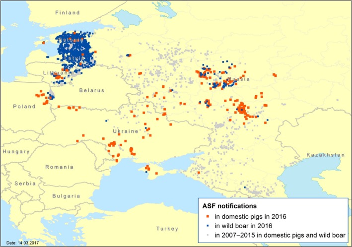
Notifications of ASF in the Eastern Europe region in 2007–2016

• Sources: ADNS, WAHIS, Official web site of the Federal Service for Veterinary and Phytosanitary Surveillance of Russia; period covered 1 January 2007–31 August 2016.

The situation on ASF in Belarus remains unclear. There were no official notifications since 2013. In 2016, the epizooty of ASF in the Russian Federation, Ukraine was characterised by an increased number of outbreaks in domestic pigs. In the Russian Federation and in Ukraine, a large number of outbreaks were notified in the domestic pig sector: 215 and 62 outbreaks, respectively. About 80% of these outbreaks have been registered in small non‐commercial pig farms where biosecurity is considered to be low. In August 2016, two outbreaks have been registered in regions of Ukraine, a further two outbreaks were registered in October 2016 in the Republic of Moldova bordering with Romania (WAHIS, 2016; not shown in Figure 1). As can be seen in Figure 1, ASF outbreaks in domestic pigs and in wild boar subpopulations can be linked or occur independently in time and space, pointing at existence of two parallel processes.

1.1. Background and Terms of Reference as provided by the requestor

1.1.1. Background

ASF is a contagious infectious disease of domestic pigs and of the wild boar, usually fatal. No vaccine exists to combat this virus. It does not affect humans nor does it affect any animal species other than members of the Suidae family.

From the beginning of 2014 up to 1/2/2016, Genotype II of ASF has been notified in Estonia, Latvia, Lithuania and Poland causing very serious concerns. The disease has also been reported in Russia, Belarus and Ukraine, which creates a constant risk for all the Member States (MS) bordering with these third countries.

There is knowledge, legislation, technical and financial tools in the European Union (EU) to properly face ASF. The EU legislation primarily targets domestic pig and addresses, when needed, lays down specific aspects related to wild boar. The main pieces of the EU legislation relevant for ASF are:

1. Council Directive 2002/60/EC3 of 27 June 2002 laying down specific provisions for the control of African swine fever and amending Directive 92/119/EEC as regards Teschen disease and African swine fever: it mainly covers prevention and control measures to be applied where ASF is suspected or confirmed either in holdings or in wild boars to control and eradicate the disease.

2. Commission Implementing Decision 2014/709/EU4 of 9 October 2014 concerning animal health control measures relating to African swine fever in certain Member States and repealing Implementing Decision 2014/178/EU: it provides the animal health control measures relating to ASF in certain Member States by setting up a regionalisation mechanism in the EU. These measures involve mainly pigs, pig products and wild boar products. A map summarising the current regionalisation applied is available online.5

3. Council Directive No 82/894/EEC6 of 21 December 1982 on the notification of animal diseases within the Community which has the obligation for Member States to notify the Commission of the confirmation of any outbreak or infection of ASF in pigs or wild boar.

The Commission is in need of an updated epidemiological analysis based on the data collected from the MS affected by ASF at the Eastern border of the EU. The use of the European Food Safety Authority (EFSA) Data Collection Framework (DCF) is encouraged given it promotes the harmonisation of data collection.

Any data that is available from neighbouring third countries should be used as well.

1.1.2. Terms of Reference

1. Analyse the epidemiological data on ASF from Estonia, Latvia, Lithuania, Poland and any other MS at the Eastern border of the EU that might be affected by ASF. Include an analysis of the temporal and spatial patterns of ASF in wild boar and domestic pigs. Include an analysis of the risk factors involved in the occurrence, spread and persistence of the ASF virus in the wild boar population and in the domestic/wildlife interface.

2. Based on the findings from the point above, review the management options for wild boar identified in the EFSA scientific opinion of June 2015 and indicate whether the conclusions of the latest EFSA scientific opinion are still pertinent.

2. Data and methodologies

This report analyses the temporal and spatial patterns of ASF in wild boar and domestic pigs, and analyses the risk factors involved in the occurrence of the ASF virus (ASFV) in the wild boar population, including the domestic/wildlife interface, based on the epidemiological data on ASF collected by Estonia, Latvia, Lithuania and Poland (Term of Reference 1). The currently available data does not allow estimating risk factors influencing the spread and persistence of ASFV. A review of the management options for wild boar identified in the EFSA scientific opinion of 2015 (Term of Reference 2) will be provided in a second scientific report in 2017.

In order to allow for comprehensive epidemiological analysis and risk assessment, data provided by the MS in accordance with Directive 82/894/EEC to the ADNS was complemented with data from MS's laboratory testing for ASF, since both positive and negative findings are of interest for epidemiological explorations.

To collect epidemiological data in a harmonised way EFSA, the Baltic States and Poland agreed on a common data model (database structure) which has been used for collecting laboratory data from the beginning of 2016.7 Details about the data model are provided in Appendix A. In June 2016, EFSA, in collaboration with its Latvian Focal Point, the Institute of Food Safety, Animal Health and Environment BIOR, organised a two‐day workshop in Riga, Latvia, with 15 participants representing veterinary services, national laboratories and research institutions, to demonstrate what kind of epidemiological analyses can be carried out using the combined data collected by the MS. The needs for collecting additional data for more comprehensive analysis were also discussed.

A specific EFSA DCF application is used to collect and validate data from laboratory testing for ASF from MS's LIMS. A summary of the data collected in the DCF is presented in Appendix B. Participants of the collaboration project (data providers and EFSA) share and use the data collated on the DCF on the basis of Data Sharing Agreements which lay down conditions of confidentiality and copyrights.

2.1. Data

2.1.1. Data for the spatio‐temporal analysis

2.1.1.1. ASF notifications

Data on ASFV detections in wild boar and domestic pigs reported between 24 January 2014 and 16 September 2016 were extracted from the ADNS. The number of outbreaks and cases are presented in Table 1.

Table 1.

Number of outbreaks in domestic pigs and cases in wild boar notified to the Animal Disease Notification System from 24 January 2014 until 16 September 2016

Country	Outbreaks in domestic pigsa	Cases in wild boar b
Estonia	24	2,249
Latvia	44	2,068
Lithuania	37	534
Poland	20	188

^aAn outbreak of African swine fever in domestic pigs refers to one or more cases of ASF detected in a pig holding.

^bA case of African swine fever in wild boar refers to any wild boar or wild boar carcass in which clinical symptoms or post‐mortem lesions attributed to ASF have been officially confirmed, or in which the presence of the disease has been officially confirmed as the result of a laboratory examination carried out in accordance with the diagnostic manual.

The ADNS database contains the exact geographical location (longitude and latitude) and the number of cases for each outbreak.

2.1.1.2. Sample‐based data

The data on ASF tests from the LIMS of the national laboratories of the Baltic States and Poland have been collected in the DCF. The data model collects individual sample data using controlled terminology and coding systems, and includes such variables as the location of sampling (longitude and latitude or lowest available level of administrative unit), the description of animal sampled (hunted or found dead), its age and sex, including the rate of decomposition of carcass if the animal was found dead, the matrices sampled, and the method of analysis (virus or antibody detection). To maintain the quality of data, EFSA is providing summary statistics for each data set submitted, focusing on data that need corrections.

The data reported to the DCF contains the information on samples tested for ASF in the period from January 2014 to June–August 2016. The LIMS data for 2016 has been collected using the agreed harmonised data model, while the data that were generated during the previous period (2014–2015), before the agreement of the harmonised data model, have been recoded as much as possible to fit the data model and allow for a joint analysis of the entire data set.

As of December 2016, information on 232,722 tests for ASF, including 85,697 tests of domestic pigs samples and 147,025 tests of wild boar samples has been collated in the DCF (Figure 2).

Figure 2.

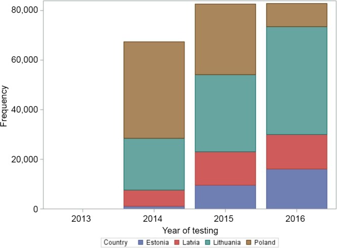
Number of tests for ASF, from January 2014 to August 2016, submitted by the Member States to the DCF

Samples were tested for ASF using polymerase chain reaction (PCR), enzyme‐linked immunosorbent assay (ELISA), immunoblotting (IB) and immunoperoxidase test (IPT) methods. The geographical distribution of the samples sampled from wild boar and notifications, based on the data for the period of January 2014–August 2016 in Estonia, Latvia and Lithuania and for the period of January 2014–June 2016 in Poland collected in the DCF and on the notifications to the ADNS during this period, is shown in Figure 3.

Figure 3.

Number of wild boar tested per 100 square km in 2014–2016 at NUTS 3 level. (A) hunted wild boar, (B) wild boar found dead

• Source: DCF.

2.1.2. Additional data used for the risk factor analysis

In this report, available data on the following risk factors potentially involved in the occurrence of the ASF virus in the wild boar population and at the domestic/wildlife interface were used for the analyses.

2.1.2.1. Environmental and demographic data

Land cover

Data on the land cover of the Baltic states and Poland were obtained from the Corine Land Cover (CLC) map 2006 (version CLC2006; European Environment Agency, Copenhagen, Denmark) with a spatial resolution of 100 × 100 m, (EEA, 1984) and converted from the raster into a percentage of wetlands, water bodies, forests, permanent crops of the total area of the administrative units, using the ArcGIS software (Spatial analyst module, Zonal statistic tool).

The data on the human population for 2015 at district (LAU 1) level have been extracted from official national statistics institutions' web sites: the Central Statistical Office of Poland (available on: http://stat.gov.pl, http://www.coloss.org/beebook, last accessed 1 August 2016), Statistics Lithuania (available on: http://www.stat.gov.lt, last accessed 1 August 2016), the Central Statistical Bureau of Latvia (available on: http://www.csb.gov.lv, last accessed 1 August 2016) and Statistics Estonia (http://www.stat.ee, last accessed 1 August 2016).

Density of settlements, national and regional roads

The locations of settlements and national and regional roads were obtained from the website of the GIS‐LAB Project (available on: http://gis-lab.info/qa/osmshp.html, last accessed 1 August 2016) for Estonia, Latvia and Lithuania and from The National Veterinary Research Institute of Poland, as shape files. They were combined with the shape files of administrative units using ArcGIS. For the analyses, the number of settlements and number of roads within each administrative unit's polygon were used.

2.1.2.2. Susceptible population data

Domestic pig population distribution

Data on the domestic pig population and distribution were provided by the MS. Table 2 provides a summary of the type of data made available to EFSA for the assessment. Data on the domestic pig population with appropriate spatial resolution and details were not available for Poland. The number of small pig farms (< 10 heads) have been used as a covariate which could characterise farms with a low level of biosecurity.

Table 2.

Data provided by the relevant member states on pig population and distribution

MS	DATA	Admin resolution	YEARS
Estonia	Pigs population size at herd level	Exact location of holdings	2014–2016
Latvia	Pigs population size Number of holdings Number of small holdings Number of sows	LAU2	2014–2016
Lithuania	Pigs population size	LAU 1	2014–2016
	Number of holdings	LAU 1	2016
Poland	Number of pigs	NUTS 3	2015

Wild boar population distribution

The size of wild boar populations (based on national hunters organisations' estimates of population size in the spring of 2014, 2015 and 2016) and the wild boar density (individuals per 1,000 ha or 10 km²) were provided by national wildlife institutions of Estonia, Latvia and Poland at ‘hunting ground’ level (Appendix D), and at NUTS3 level for Lithuania. The data provided by Estonia include also yearly numbers of hunted wild boar, wild boar road kills and wild boar found dead. All data were recoded to administrative unit level using generation of random points and spatial aggregation using ArcGIS.

2.1.2.3. Aggregation of data

For each administrative unit, the areal percentage of the different types of land cover, human population, wild boar and domestic pig population were considered as potential influencing covariates in the risk factor analysis. All covariates were aggregated spatially on the basis of the shape file of the administrative units at three different levels: NUTS 3, LAU 1 and LAU 2.

2.1.3. Summary of data used in the risk factor analysis

Information regarding available potential risk factors were transformed in order to use them in the risk factor analysis considering a common scale. The list of available risk factors provided by MS involved in the assessment is summarised in Table 3.

Table 3.

Available risk factors provided by Member States involved in the assessment

Potential risk factor	Abbreviation	Latvia	Estonia	Lithuania	Poland
Human population proportion	HPPrp	X	X	X	O
Proportion of the number of roads	RdsPrp	X	X	X	X
Proportion of number of settlements	StlmPrp	X	X	X	X
Forest area proportion	FrstPrp	X	X	X	X
Water bodies area proportion	WtrbdsPrp	X	X	X	X
Percentage of area of wetlands	PrcnWtlnd	X	X	X	X
Percentage of are of inland wetlands	PrcInWtln	X	X	X	X
Wild boar density (ind./10 km2)	WBDens	X	X	X	X
Proportion of number of pig farms	PrpNmPgFrms	X	X	O	O
Proportion of number of pigs	PrpNmPg	X	X	X	O
Proportion of small pig farms (less than 10 animals)	PrpPgFms1_10	X	X	O	O
Proportion of number of pigs in small pig farms (less than 10 animals)	PrpNmPgs_1_10	O	X	O	O

X: available; O: not available.

The information provided were transformed to relative proportions considering the spatial resolutions used in the risk factor analysis for each MS, using the maximum value reported for all years as the reference point, and considering the ratio of each region value with respect to the maximum value reported.

Relative proportions in a given region were calculated for:

• Geographical Factors

  • –Number of roads (number of asphalted roads)
  • –Forest area (area of broad‐leaved forest, coniferous and mixed forest)
  • –Number of settlements (number of settlements (dots) within administrative unit)
  • –Water bodies (area of water courses, water bodies, coastal lagoons and estuaries)

• Population Characteristics

  • –Human Population (total number of people)
  • –Number of pigs (total number of pigs)
  • –Number of pig farms (total number of pig holdings)
  • –Number of small pig farms (number farms with less than 10 animals)
  • –Number of pigs in small farms (total number of pigs kept in small pig farms).

Also, the proportion of area of maritime wetlands (salt marshes, salines and intertidal flats) and inland wetlands (inland marshes and peat bogs) were calculated, considering the area of the region as the denominator and later convert it to percentages.

Wild boar density was calculated using the number of animals divided by the area of the region divided by 10, to express it as a function of 10 km² (or 10,000 ha).

2.2. Methodologies

Data from the DCF were extracted and collated using analytics software SAS Enterprise Guide 5.1 (http://www.sas.com/) before carrying out the analyses described in detail below.

2.2.1. Spatio‐temporal analysis

Data processing and visualisation of spatio‐temporal spread of the disease in the wild boar populations were performed using geographic information system software ArcGIS 10.2 (http://www.esri.com/). An analysis of clusters was carried out to visualise local spread of the virus. A cluster is defined as a group of ASF notifications in wild boar which are temporally and spatially linked. For the explicit spatial clusters established in the previous period (January 2014–April 2015), that have been described in the EFSA scientific opinion on ASF (EFSA AHAW Panel, 2015), as well as in the clusters formed in the subsequent period (up to September 2016), the mean centre and standard distance were defined by corresponding tools of the Spatial analyst module of Arc Map 10.2.

The mean centre identifies the geographic centre (or the centre of concentration) for a set of features (longitude and latitude values). The standard distance measures the degree to which features are concentrated or dispersed around the geographic mean centre (1 standard deviation). These two parameters were defined by corresponding tolls of the Spatial Analyst module of Arc Map 10.2.

Statistical models that deal with data that is collected across space (i.e. different regions) and possibly over time (i.e. different years) have been used. The analysis of such data types takes into account the spatial and/or temporal dependence of the observations. The linear component of the spatio‐temporal model for the binary data for the presence of ASF (ASF status, time and location) can be written including a random effect accommodating temporal dependence, and another one to account for spatial dependence, as well as the possibility to include potential interactions between space and time. Therefore, the Besag, York and Mollie's (BYM) model was fitted to the spatial effect. The BYM model takes into account not only the spatial autocorrelation present in the data, but it also assumes that the estimates obtained between areas are independent of each other. The spatial effect of the BYM model assumes that the expected value of each area depends on the values of the neighbouring areas (in this case areas sharing boundaries). Thus, areas close together are considered to be more similar than areas that are far apart. In this application, it was assumed that the structured and unstructured effects are not independent of each other (Riebler et al., 2016). Thus, the model was written considering a mixture formulation in which it reduces to pure overdispersion (spatially unstructured), if the mixture parameter is estimated to be 0, or to the intrinsic conditionally autoregressive (ICAR)/Besag model when the mixture parameter is equal to 1. Thus, the proportion of the marginal variance explained by the spatial effect is given by the mixture parameter. The spatio‐temporal interaction term addresses the relationship between the temporal and spatial trend, and different types of interaction were explored. This model was used considering regions to be positive if at least one ASF case was notified, and the spatio‐temporal model was built to model the relationship between potential risk factors and case notification in a region as well as the time evolution of case notification.

Epidemic curves were constructed using Microsoft Excel.

The spatial distribution of ASF cases in wild boar and outbreaks in domestic pigs was analysed by cluster, on the basis of data extracted from the ADNS database for the period of January 2014–September 2016, containing the exact geographic location (longitude and latitude) and other attributes, including the number of cases. This was based on the date of laboratory confirmation (the date of initial detection is not available for wild boar cases in ADNS). Data were collated in MS Excel and displayed in Arc Map 10.2.

The temporal distribution of ASF cases in wild boar was analysed by country on the basis of data extracted from the DCF based on the date of sampling.

The apparent prevalence is the number of animals testing positive by a diagnostic test divided by the total number of animals (samples) tested.

To evaluate if potential variations in the apparent viral prevalence in hunted and found dead wild boar, and in the apparent antibody prevalence in hunted wild boar exist, data obtained from PCR and ELISA tests carried out on samples from wild boar during the period of January 2014–August 2016 were analysed statistically using a 95% confidence interval (CI). In order to obtain more precise results, a statistical model with a smooth‐time component developed in R software environment for statistical computing and graphics (version 3.3.1, https://www.r-project.org) was used.

2.2.2. Risk factor analysis

In order to estimate the probability of ASFV presence in wild boar populations and the potential relationship between environmental and biological factors with its presence, logistic/classification tree models were used. For classification trees, variable importance based on the pruned tree as proposed by Breiman et al. (1984) was used. Details on the methodology used can be found in Appendix E.

All variables related to host availability (number of small pig holdings and wild boar population distribution and density (i.e. individuals/10 km²), human population (density of settlements, national and regional roads) and landscape (percentage of wetlands, water bodies, forests, permanent crops of the total area of the administrative units), were considered as potential explanatory variables when constructing the logistic/classification tree models. Multicollinearity between predictor variables was not studied in detail.

Anthropogenic risk factors linked to human activities (e.g. control measures, number of hunted or disposed carcasses, etc.), and biological risk factors related to the virus (e.g. contagiousness or virulence of the virus) were not assessed in this report.

The model was used to assess if the available geographical and population variables are potentially associated with the occurrence of ASFV in a wild boar population in a given region, in order to generate hypothesis of potential factors that could be influencing the spread of the disease.

When building regression models, collinearity between covariates/predictors/risk factors is a common phenomenon, which hampers the interpretation of the coefficients in the regression models, given the relation that might exist between two or more covariates included in the model. However, for prediction purposes, the collinearity issue does not play a major role. The focus of this report was the investigation of all potential factors that could be related to the outcome of interest (i.e. the presence of ASF cases in a region), but not on estimating the specific effect of any covariate in particular. The expected effect of multicollinearity in this context is that redundant factors might be included as potential modifiers. Yet, they are acting only through other factors already included. As the main purpose here is to have an exhaustive list of all potential risk factors, the presence of redundant predictors is considered acceptable for this report. Before conducting further experiments and modelling in the next scientific report, an investigation of the potential risk factors to be included needs to be carried out.

All models were fitted on a yearly basis to study the effect of geographical factors on the probability of observing ASF‐positive cases in a given region, and how they might change over time.

For Estonia, Latvia and Lithuania, the models were identifying potential risk factors that could be associated with the occurrence of ASF (i.e. at least one positive PCR test) in a region. The modelling results are shown in Section 3.1.3. In the case of Poland, given the limited information available, no clear indications of any association between the risk factors studied and the virus presence were found. In order to explore this further, several models were applied to the data, i.e. machine learning methods (random forest (Breiman, 2001), support vector machine (Scholkopf and Smola, 2002), ROSE (Lunardon et al., 2014)) as well as generalised linear models. None of the models used produced an acceptable fit, therefore no conclusions could be drawn at this stage.

3. Results

3.1. Descriptive epidemiology

3.1.1. Spatio‐temporal patterns of spread of ASF in the Baltic countries and Poland

By August 2016, the total number of notifications in the ADNS in wild boar was 5,039 (97.6%), and 125 in domestic pigs (2.4%). The evolution of ASFV spread in the regions of ASF‐affected EU MS is shown in Figure 4.

Figure 4.

Evolution of ASF in wild boar in the Baltic states and Poland from July 2014 to September 2016 (note that map E covers the period 1 July–16 September 2016)

• Source: ADNS.

3.1.1.1. Temporal distribution

The temporal distribution of ASF‐positive results of laboratory tests (PCR) carried out on wild boar (hunted and found dead) by the national laboratories of the Baltic States and Poland and reported to the DCF is shown in Figure 5.

Figure 5.

Number of positive samples (PCR) identified in wild boar (hunted and found dead) between December 2013 and August 2016 in the Baltic countries and Poland submitted to the DCF

• Start of active selective hunting of female wild boars and removal of dead animals in Latvia;
  Start of active selective hunting of female wild boars and removal of dead animals in Estonia;
  Start of active selective hunting of female wild boars and removal of dead animals in Lithuania;
  Start of active selective hunting of female wild boars and removal of dead animals in Poland (Appendix D).

The numbers of ASFV‐positive samples of wild boar in the EU MS were not randomly distributed throughout the year (Figure 5). Although quite variable, the number of positive samples showed generally a consistent pattern between countries, with more positive samples in summer and winter.

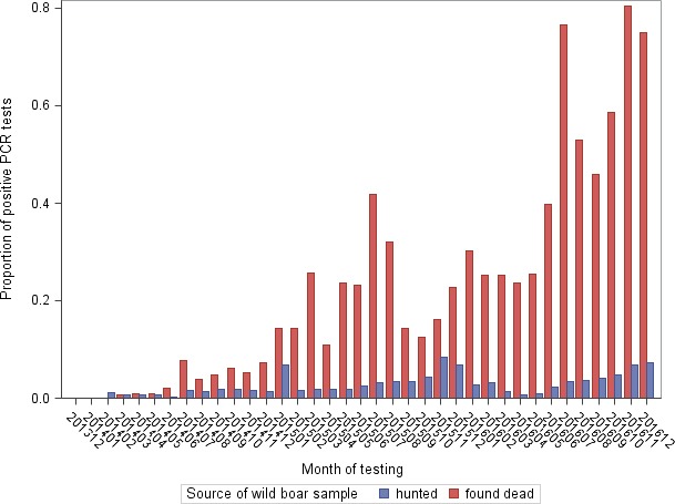
Figure 6 differentiates the number of tested and positive samples in hunted wild boar and wild boar found dead in the Baltic States and Poland. The figure illustrates that there is a clear peak in the number of positive samples in winter in the hunted animals, which is not explicit in the wild boar that are found dead. This indicates that the winter increase is potentially driven by human activity patterns (significant hunting activity over winter). In animals found dead, a peak of positive cases is seen in summer. This could be related to the epidemiology of the disease in wild boar and/or the biology of wild boar; however, this needs further investigation.

Figure 6.

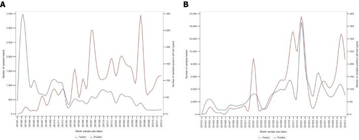
Temporal distribution of tested and positive samples in wild boar found dead (A) and in hunted wild boar (B) in the Baltic States and Poland (January 2014–September 2016)

• Note that the scales of the tested and the positive hunted wild boar in Figure B are different from the corresponding scales in Figure A.
  Source: DCF.

3.1.1.2. Spatial distribution

The spatial distribution of ASF in the Baltic countries and Poland is characterised by a concentrated distribution of notifications rather than an equal distribution of notifications. Hot‐spots of wild boar cases which are linked in space and time can be described as a cluster. Characteristics of the main clusters which were observed until May 2015 in the affected EU countries were given in the last Scientific Opinion on ASF of EFSA (EFSA AHAW Panel, 2015).

Several new clusters formed over the past year (May 2015–September 2016) (Figure 7). There are four new clusters of ASF notifications in wildlife in Estonia, including the cluster of two cases in wild boar on Saaremaa Island. Given the fact that there is no continuous wild boar population and no wild boar migration between the island and the mainland of Estonia, a non‐anthropogenic nature of the introduction of the virus on the island can be excluded.

Figure 7.

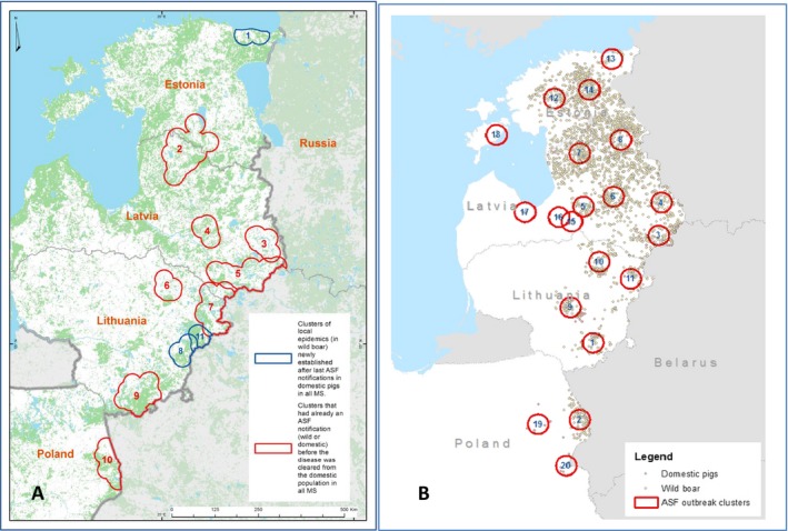
Temporality of clusters of notifications in the four affected EU Member States in the period from July 2014 to May 2015 (A) and in the period from June 2015 to September 2016

• Red clusters: ASF clusters involving wild boar or domestic pigs which were preceded by an outbreak in the domestic pig sector and had a notification before the domestic pig outbreak had been resolved; Blue clusters: ASF clusters which are not preceded by outbreaks in the domestic pig sector and had no notification before the domestic pig outbreak had been resolved.

Figure 8 demonstrates the distribution in time of notifications in wild boar (blue dots) and domestic pigs (orange dots) in each cluster.

Figure 8.

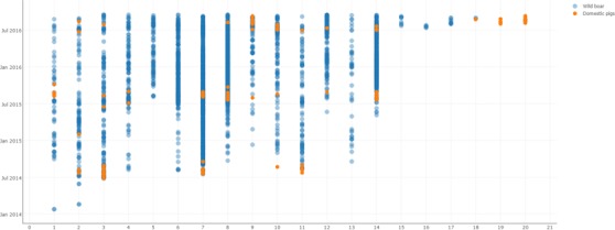
Temporal distribution of ASF notifications in wild boar (blue) and domestic pigs (orange) on spatial clusters in the four affected EU Member States from January 2014 to September 2016

• Source: ADNS.

The interaction between wild boar and domestic pig subpopulations in the context of ASFV spread might be characterised by the notification of the outbreak in the domestic pig sector on Saaremaa Island in Estonia, which was followed by a nearby case in wild boar (Figure 8, cluster 18). It is considered that the virus was introduced to the domestic pig farm indirectly, most likely by humans disregarding the biosecurity rules and procedures in place. Based on epidemiological investigations, the source of the infection for this farm is considered to be infected dead wild boar found in a radius of 10 km from the farm which had not yet been detected by the time the outbreak occurred (Arvo Viltrop, personal communication).

Detailed spatial characteristics of some of the main existing clusters are given below (Figure 9).

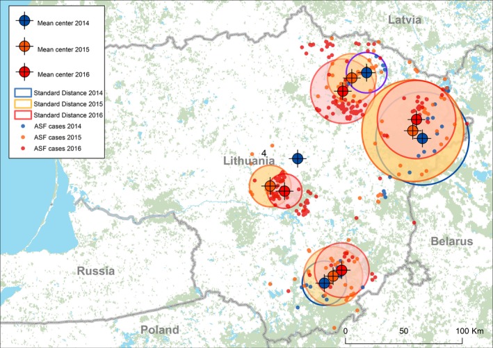
Figure 9.

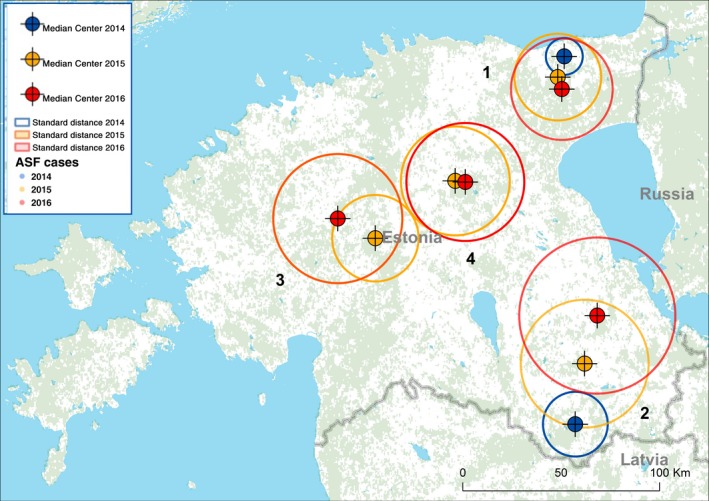
Mean centres and standard distances (1 standard deviation of distances between individual notifications and the centre of a cluster) of the notifications of ASF in wild boar in Estonia, January 2014–August 2016

• Source: ADNS.

3.1.1.3. Spatio‐temporal characteristics of ASF spread in Estonia

The distance between the mean centres of the distribution of the ASF notifications of the southern cluster in Estonia (number 2, Figure 9) bordering with the Russian Federation and Latvia are shown in Table 4 for the years 2014, 2015 and 2016 in Estonia, as well as the standard distances of the distribution of ASF notifications towards the centres in the same years.

Table 4.

Yearly distance between mean centres and the standard distances of the distribution of ASF notifications in wild boar towards the centres of the clusters in the years 2014, 2015 and 2016 in Estonia

Cluster (Figure 9)	Distance between mean centres, km		Standard distance, km (1 SD)
	2014–2015	2015–2016	2014	2015	2016
1	11.0	6.5	9.0	22.2	25.8
2	31.0	25.0	16.5	32.5	39.5
3	–	21.7	–	22.2	32.9
4	–	5	–	27.7	30.0

Another parameter that characterises a cluster from the perspective of its longevity and size is the average distance between the notification of the index case and the following cases (Table 5).

Table 5.

Average distances between notification of index and following cases of clusters in wild boar in Estonia

Cluster (Figure 9)	Average distance (km)			Start
	2014	2015	2016
1	5.4	17.5	26.5	09/2014
2	3.6	40.5	57.4	10/2014
3	–	16.6	38.5	05/2015
4	–	23.5	33.7	07/2015

Based on these observed average distance values, the average speed of propagation of ASF in Estonia is estimated to be about 2 km/month. A detailed analysis of possible factors influencing ASFV propagation requires additional data.

The BYM model was used to evaluate the influence of potential risk factors on the spatio‐temporal pattern observed. The model used considers regions to be positive if at least one ASF case was notified, and the spatio‐temporal model was built to model the relationship between potential risk factors and case notification in a region as well as the time evolution of case notification. Among the 12 potential risk factors, the model identified wild boar density as the only factor having a significant effect, when considering the spatio‐temporal characteristics of the data. The model results are shown in Figure 10.

Figure 10.

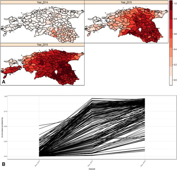
Modelling outputs, fitted values for each region and timepoint. Mean estimated probability for the temporal profiles for each LAU2 region (time evolution of the estimated probability of observing ASF cases for each LAU2 region, B) and their estimated spatial pattern for each year (yearly map of the estimated probability of observing ASF cases in each region, A)

The model results indicate that in Estonia wild boar density is proportional to the likelihood of observing ASF cases in a region, i.e. the larger the wild boar density, the larger is the likelihood to observe ASF cases in a region. The estimated value of the mixture parameter was 0.934 (credible interval of 0.763–0.997), indicating a strong spatial effect, as also shown in the maps in Figure 10A. The estimated spatial variability was 1.54, with a credible interval of 0.74 and 2.81, corroborating the strong spatial effect. The temporal effect shows in general a significant increase in probability of observing ASF cases in a region (likelihood of notification in a region), considering a model that allows each region to have a different time profile for the likelihood of observing ASF cases (Figure 10B). This is expected in general in a spatially expanding phenomenon.

3.1.1.4. Spatio‐temporal characteristics of ASF spread in Latvia

A similar analysis of the data on ASF notifications has been performed for Latvia. It should be noted that Estonia and Latvia have one common cluster (cluster 2, Figure 11) and it has been considered with the other clusters on the territory of Latvia (Figure 11).

Figure 11.

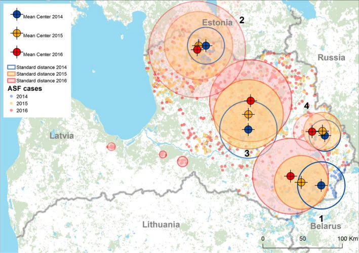
Mean centres and standard distances (1 standard deviation from the centre of a cluster) between notifications of ASF in wild boar in Latvia during the period of January 2014–August 2016

• Source: ADNS.

In 2015, spread of ASFV in the wild boar population was observed in the same territories of Latvia infected in 2014. During the summer of 2016, further spread of ASFV in the wild boar population occurred, covering about 70% of the country (Figure 11). By the end of August 2016, 765 cases in wild boar and two outbreaks in small pig farms had been registered.

Clusters on the territory of Latvia in 2016 are characterised by large standard distances and a relatively limited movement of the geographic mean centres of the clusters. A more detailed description of these parameters is presented in Table 6.

Table 6.

Distance between the yearly mean centres and the standard distances of the distribution of ASF notifications towards the centres of the clusters in wild boar in the years 2014, 2015 and 2016 in Latvia

Cluster (Figure 11)	Distance between mean centres, km		Standard distance, km (1 SD)
	2014–2015	2015–2016	2014	2015	2016
1	25.5	15.5	29.8	33.9	47.8
2	10.7	5.2	22.7	42.6	60.1
3	19.3	17.6	36.0	43.8	52.0
4	6.7	12.9	19.6	23.6	23.6

Cluster 3 is the most ‘mobile’ with an average distance of the periphery from the starting point of 67.8 km and an average of 2.8 km/month of propagation (Table 7). The density of wild boar in the regions affected by this cluster was estimated to be relatively high in 2015 and 2016, which might explain the larger average distances between index and consecutive cases observed in this particular area of Latvia.

Table 7.

Average distances between index and following cases of clusters in wild boar in the years 2014, 2015 and 2016 in Latvia

Cluster (Figure 11)	Average distance (km)	Average distance (km)	Average distance (km)	Start, month
	2014	2015	2016
1	15.9	40.3	54.8	06/2014
2	6.0	29.3	41.1	07/2014
3	29.8	53.9	67.8	08/2014
4	17.7	25.2	23.8	08/2014

The spatio‐temporal model (BYM) does not provide insights on potential risk factors that could be linked to the presence of ASF cases in a given region of Latvia; therefore, the results of the model are not shown. Additional models (see Section 2.2.2) were used to identify potential risk factors. Results are presented in Section 3.1.3.

3.1.1.5. Spatio‐temporal characteristics of ASF spread in Lithuania

Spatial distribution of clusters, yearly mean centres and standard distances (1 standard deviation from the centre of cluster) between notifications of ASF in wild boar in Lithuania are presented in Figure 12.

Figure 12.

Mean centres and standard distances (1 standard deviation from the centre of cluster) between notifications of ASF in wild boar in Lithuania in the period of 2014–2016

Analysis of these parameters demonstrates that the pattern of spatial distribution and propagation of the virus in Lithuania partly differs from the previously discussed countries. Yearly movements of the mean centres of these clusters and standard distance are limited, with the exception of the cluster which is located on the borders with Latvia and Belarus.

Table 8.

Yearly distance between median centres and standard distances of distribution of ASF notifications in wild boar towards centres of clusters in Lithuania in 2014–2016

Cluster (Figure 12)	Distance between mean centres, km		Standard distance, km (1 SD)
	2014–2015	2015‐2016	2014	2015	2016
1	9.5	18.9	18.9	25.3	23.2
2	11.3	15.5	39.7	43.7	33.3
3	13.5	13.6	17.2	20.7	27.8
4	33.3	13.5	–	18.0	14.6

Table 9.

Average distances between index and following cases of clusters in Lithuania

Cluster (Figure 12)	Average distance (km)	Average distance (km)	Average distance (km)	Start, month
	2014	2015	2016
1	18.4	31.1	34.9	01/2014
2	–	36.9	32.2	07/2014
3	20.0	19.0	28.3	11/2014
4		17.3	18.4	12/2014

The distance from the starting point up to the periphery of the clusters suggests that the estimated speed of spread of ASF in Lithuania of approximately 1 km/month is lower than in the other Baltic countries.

Given the limited information provided, the spatio‐temporal model (BYM) considering potential risk factors that could be linked to the presence of ASF cases in a given region was not feasible. Results of the models are not shown, other modelling techniques described in Section 2.2.2 were used instead. Results of these analyses are presented in Section 3.1.3.

3.1.1.6. Spatio‐temporal characteristics of ASF spread in Poland

Poland registered ASF in the wild boar population close to the border with Belarus in late winter 2014. Since then the epizooty showed limited spread in the wild boar population, mainly in the area adjacent to the Belarus border (Figure 13).

Figure 13.

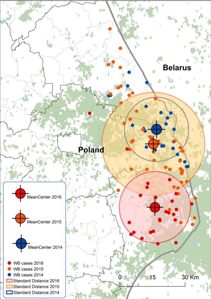
Mean centres and standard distances (1 standard deviation from the centre of cluster) between notifications of ASF in wild boar in Poland during the period 2014–2016

The average distance between the index case notification and following cases in wild boar in Poland were 24.5, 33.6 and 58.7 km, respectively, and the distances between yearly mean centres (2014–2015 and 2015–2016) were 7.2 and 28.9 km, respectively.

In summary, the ASF outbreaks in wild boar in Estonia, Latvia, Lithuania and Poland show the spatio‐temporal pattern of a small‐scale epidemic.

Given the limited number of cases reported, the spatio‐temporal model (BYM) considering potential risk factors that could be linked to the presence of ASF cases in a given region was not appropriate. Other modelling techniques described in Section 2.2.2 were used instead, results are presented in section 3.1.3.

3.1.2. Virus (PCR) and ASFV‐antibody prevalence time trends

The virus (PCR) prevalence in hunted wild boar (A) and wild boar found dead (B) at country level in the period from January 2014 to August 2016 are presented in Table 10.

Table 10.

Apparent Virus (PCR) prevalence in wild boar in the Baltic countries and Poland, January 2014 to August 2016 (percentage; source: DCF)

	2014		2015		2016
Country	Wild boar found dead	Wild boar hunted	Wild boar found dead	Wild boar hunted	Wild boar found dead	Wild boar hunted
Estonia	29.8a	1.01a	71.41	3.8	85.7	3.0
Latvia	53.2	0.68	73.08	1.8	78.2	2.1
Lithuania	23.8	0.11	27.3	0.97	59.9	0.13
Poland	1.4c	0.04b	1.42c	0.1b	0.5c	0.0b

n/a: data are not available.

^aSamples from a period the infection was not detected in a country are included.

^bMost of the samples tested originate from affected administrative units (see Figure 3A).

^cA large proportion of samples tested originate from unaffected administrative units (see Figure 3B).

The highest virus (PCR) prevalences in wild boar found dead was observed in Estonia (85.7% of all tested carcasses) and Latvia (78.2%), a lower prevalence was found in Lithuania (59.9%), while in Poland the virus (PCR) prevalence in wild boar that were found dead was very low with 0.5% at country level, and varied from 4.6 to 31.3 in affected NUTS3 regions. However, it should be noted that most of the samples from hunted wild boar tested by Poland originate from affected administrative units, and a large proportion of samples tested from wild boar found dead by Poland originate from unaffected administrative units, which may cause an artificial lowering of the apparent prevalence as compared to the other countries (see also Figure 3A and B). In contrast, the virus (PCR) prevalence in hunted wild boar remained very low in all countries and did not exceed 3.8%.

As the wild boar populations of the Baltic countries and Poland constitute overlapping metapopulations, rather than separate entities, the territory inhabited by these metapopulations can be considered as a single ASF‐affected region of about 500,000 km². Therefore, the overall monthly prevalence has also been calculated for the affected countries as a whole (Figure 14). The average monthly prevalence (proportion of positive samples to all tested samples in wild boar hunted and wild boar found dead) in this region shows an increasing trend over time (Figure 14).

Figure 14.

Average monthly apparent virus (PCR) prevalence in the Baltic countries and Poland in hunted wild boar and wild boar found dead, January 2014–December 2016

• Source: DCF.

3.1.2.1. Time Trends by country

Estonia

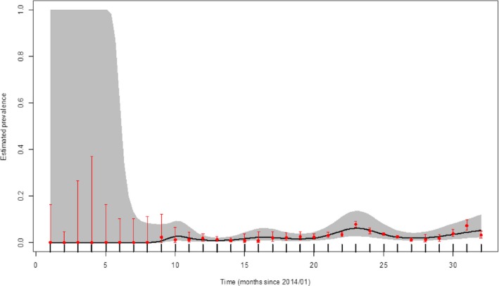
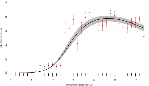
The monthly dynamic of the apparent virus (PCR) prevalence in wild boar found dead in Estonia from the period from January 2014 to August 2016 is presented in grey colour – 95% confidence interval (CI‐95%) (Figure 15).

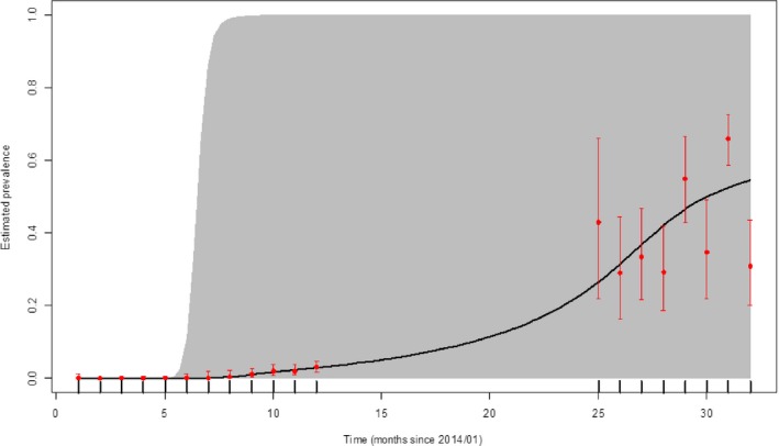
Figure 15.

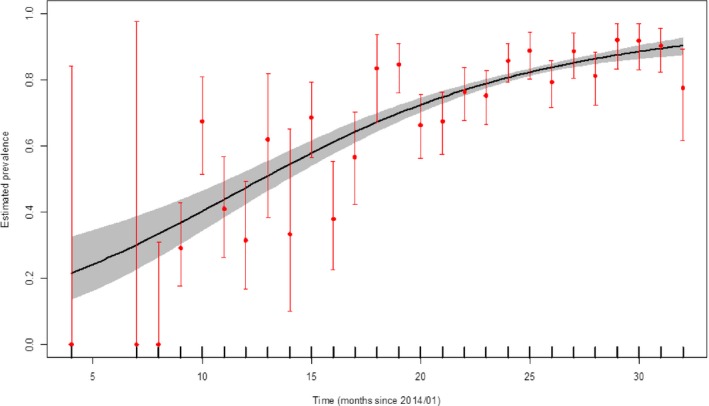
Apparent virus (PCR) prevalence in wild boar that were found dead during the period from January 2014 to August 2016 in Estonia

• Grey colour: 95% confidence interval (CI‐95%).

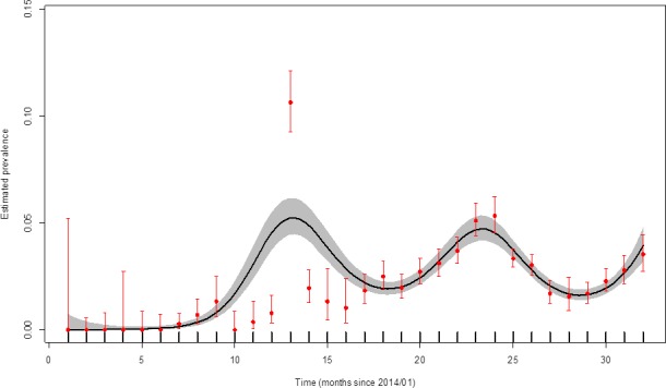
During this period, the apparent virus (PCR) prevalence in hunted wild boar is low in Estonia and shows no distinguished temporal trend (Figure 16). The confidence intervals were constructed based on the number of observations reported in each month for the whole reporting period. Their width reflects the number of observations reported. When confidence intervals are wide, such as seen in Figures 15, 20 and 24, the total number of observations reported for that month is rather low, indicating the uncertainty on the inference that could be made for that specific period.

Figure 16.

Apparent virus (PCR) prevalence in hunted wild boar in Estonia (2014–2016)

• Grey colour: 95% confidence interval (CI‐95%).

Figure 20.

Apparent ASFV‐antibody prevalence in hunted wild boar in Latvia (January 2014–August 2016)

• Grey colour: 95% confidence interval (CI‐95%).

Figure 24.

Apparent virus (PCR) prevalence in wild boar found dead in Poland (January 2014–August 2016)

• Grey colour: 95% confidence interval (CI‐95%).

A statistical analysis of the apparent antibody prevalence in Estonia from September 2014 to August 2016 is shown in Table 11.

Table 11.

ASFV‐antibody prevalence in affected regions of Estonia (2014–2016)

Region	Ab prevalence,%	LBa	UBa
Põhja‐Eesti	0.0049	0.0016	0.0115
Lääne‐Eesti	0.0094	0.0059	0.0142
Kesk‐Eesti	0.0138	0.0112	0.0169
Kirde‐Eesti	0.0362	0.026	0.049
Lõuna‐Eesti	0.0291	0.0256	0.033

^aLB: lower bound of 95% confidence interval, UB: Upper bound of 95% confidence interval.

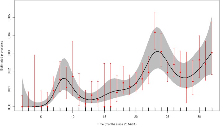
Figure 17 demonstrates the time trend of apparent antibody prevalence in hunted wild boar in affected regions in Estonia.

Figure 17.

Apparent ASFV‐antibody prevalence in hunted wild boar in Estonia (January 2014–August 2016)

• Grey colour: 95% confidence interval (CI‐95%).

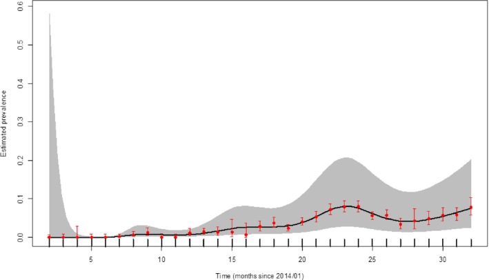
Latvia

Figures 18 and 19 demonstrate the time trend of the apparent virus (PCR) prevalence in wild boar in affected regions in Latvia, either found dead or hunted, respectively.

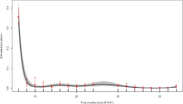
Figure 18.

Apparent virus (PCR) prevalence in found dead wild boar in Latvia (January 2014–August 2016)

• Grey colour: 95% confidence interval (CI‐95%).

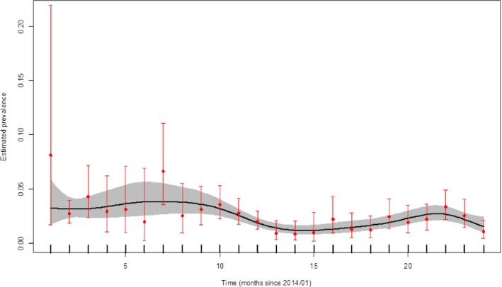
Figure 19.

Apparent virus (PCR) prevalence in hunted wild boar in Latvia (January 2014–August 2016)

• Grey colour: 95% confidence interval (CI‐95%).

The statistical analysis of the apparent ASFV‐antibody prevalence in Latvia from September 2014 to August 2016 is shown in Table 12.

Table 12.

Apparent antibody prevalence in hunted wild boar (serum) in Latvia (2014–2016, CI‐95%)

Region	Ab prevalence	LBa	UBa
Kurzeme	0	0	0.0066
Latgale	0.0374	0.0335	0.0417
Pierīga	0.051	0.0424	0.0609
Vidzeme	0.0444	0.0408	0.0483
Zemgale	0.0296	0.0237	0.0364

^aLB, UB: lower and upper bound of 95% confidence interval.

Figure 20 demonstrates the time trend of the apparent ASFV‐antibody prevalence in hunted wild boar in affected regions in Latvia.

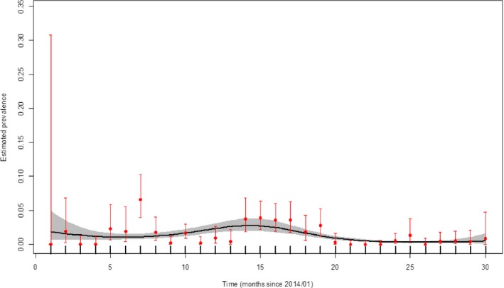
Lithuania

The apparent virus (PCR) prevalence in wild boar which were found dead or which were hunted in Lithuania from the period from January 2014 to August 2016 are presented in Figures 21 and 22, respectively.

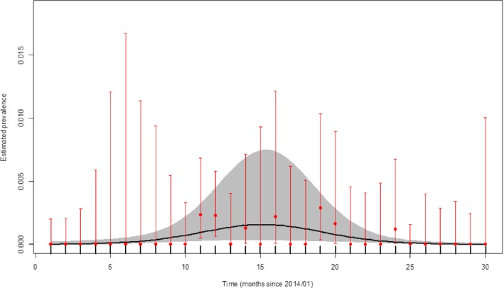
Figure 21.

Apparent virus (PCR) prevalence in wild boar found dead in Lithuania (January 2014–August 2016)

• Grey colour: 95% confidence interval (CI‐95%).

Figure 22.

Apparent virus (PCR) prevalence in hunted wild boar in Lithuania (January 2014–August 2016)

• Grey colour: 95% confidence interval (CI‐95%).

The exploratory analysis of the apparent ASFV‐antibody prevalence in Lithuania from September 2014 to August 2016 is shown in Table 13.

Table 13.

Apparent ASFV‐antibody prevalence in hunted wild boar in 2014–2016 in Lithuania

Region	ELISAPrev	LBa	UBa
Alytaus apskritis	0.0617	0.0478	0.0781
Kauno apskritis	0.0092	0.0065	0.0125
Klaip≐dos apskritis	0	0	0.0131
Marijampol≐s apskritis	0.0027	1.00E‐04	0.015
Panev≐žio apskritis	0.0427	0.0334	0.0536
Šiaulių apskritis	0.0022	1.00E‐04	0.0122
Taurag≐s apskritis	0	0	0.0125
Telšių apskritis	0	0	0.0115
Utenos apskritis	0.0264	0.021	0.0326
Vilniaus apskritis	0.0149	0.0106	0.0204

^aLB, UB: lower and upper bound of 95% confidence interval.

Figure 23 demonstrates the time trend of the apparent ASFV‐antibody prevalence in hunted wild boar in affected regions in Lithuania.

Figure 23.

Apparent ASFV‐antibody prevalence in hunted wild boar in Lithuania, 2014–2016

• Grey colour: 95% confidence interval (CI‐95%).
  Source: DCF.

Poland

The apparent virus (PCR) prevalence in wild boars which were found dead or which were hunted in Poland from the period from January 2014 to August 2016 is presented in Figures 24 and 25, respectively.

Figure 25.

Apparent virus (PCR) prevalence in hunted wild boar in Poland (2014–2016, DCF)

• Grey colour: 95% confidence interval (CI‐95%).

The statistical analysis of the apparent ASFV‐antibody prevalence in Poland from September 2014 to August 2016 is shown in Table 14.

Table 14.

Apparent ASFV‐antibody prevalence in hunted wild boar in Poland (January 2014–August 2016)

Region	Seroprevalence	LBa	UBa
PL116	0	0	0.975
PL127	0	0	0.8419
PL12A	0	0	0.8419
PL12E	0.0342	0.0112	0.0781
PL311	0.0071	0.0015	0.0205
PL312	0.0489	0.0276	0.0793
PL314	0.037	0.0077	0.1044
PL315	0	0	0.8419
PL323	0	0	0.1951
PL324	0.0523	0.0228	0.1004
PL325	0	0	0.6024
PL326	0	0	0.8419
PL331	0	0	0.975
PL343	0.0225	0.0186	0.027
PL344	0.0206	0.0169	0.025
PL345	0.0317	0.0223	0.0436
PL524	1	0.025	1
PL616	0	0	0.975
PL617	0	0	0.975
PL621	0	0	0.8419
PL622	0	0	0.6024
PL623	0	0	0.8419
PL638	0	0	0.975

^aLB, UB: lower and upper bound of 95% confidence interval.

Figure 26 demonstrates the time trend of the apparent ASFV‐antibody prevalence in hunted wild boar in affected regions in Poland.

Figure 26.

Apparent ASFV‐antibody prevalence in hunted wild boar in Poland (January 2014–August 2016)

• Grey colour: 95% confidence interval (CI‐95%).

In summary, there is no clear time trend in ASFV‐antibody prevalence in hunted wild boar.

Virus prevalence in hunted wild boar is very low with apparent prevalence values ranging between 0.5% and 3%, without any apparent trend over time. Apparent virus prevalence in wild boar found dead in Estonia, Latvia and Lithuania ranges from 50% to 90%, with the exception of Poland, where values between 1% and 4% were observed.

Since the beginning of the epidemic, the apparent antibody prevalence in hunted wild boar has always been lower than the apparent virus prevalence in hunted wild boar, indicating an unchanged epidemiological/immunological situation.

The apparent virus (PCR) prevalence in wild boars which were found dead and which were hunted in three Baltic countries (Estonia, Latvia and Lithuania) from the period from January 2014 to August 2016 is presented in Figures 27 and 28, respectively.

Figure 27.

Apparent virus (PCR) prevalence in wild boar found dead in the Baltic countries (January 2014–August 2016)

Figure 28.

Apparent virus (PCR) prevalence in hunted wild boar in the Baltic countries (2014–2016, DCF)

3.1.3. Evaluation of the risk factors contributing to the African swine fever occurrence

In order to understand the effect of geographical and population factors on the probability of observing at least one ASF‐positive case in a given region, all analyses were performed for each country for each year separately, except for Lithuania, for which the analysis was carried out for the 3‐year period 2014–2016.

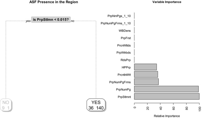
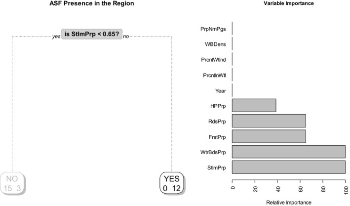
The results of the different models have been presented graphically (see Figures 28, 29, 30, 31, 32). The bar plot (right side) shows the relative importance of the covariates considered in the analysis, and the longer the bar, the higher the importance (i.e. the stronger the association with the presence of ASF in the area of interest). Being a relative importance, the bar at the bottom always reaches the 100% value, and all other values relate to this reference.

Figure 29.

Apparent ASFV‐antibody prevalence in hunted wild boar in the Baltic countries (January 2014–August 2016)

Figure 30.

Probability tree and relative importance of variables for detection of ASF in wild boar in Estonia (for 2015)

Figure 31.

Probability tree and relative importance of variables for detection of ASF in wild boar in Estonia (for 2016)

Figure 32.

Probability tree and relative importance of variables for detection of ASF in wild boar in Latvia (for 2014)

3.1.3.1. Estonia

Year 2014

The model did not find any of the risk factors to be able to explain the likelihood to observe ASF‐positive cases within a region.

Year 2015

The model result indicates that all potential risk factors contribute to the presence of ASF cases. The main factors influencing the notification of ASF cases within a region are the relative proportion of pigs (PrpNumPg), forest (PrpFrst), human settlements (PrpStlm) and pig farms (PrpNumPgFrms) (Figure 30).

The sensitivity achieved by the model is around 84%, and the overall error is below 12% when cross‐validation is used. Cross‐validation is used to have an honest evaluation of model performances, in which the data is subdivided randomly in k subsets and k − 1 subsets are used to fit the model while the left out subset is used to evaluated the model, and the process is repeated until all subsets has been used to evaluate the model.

Year 2016

The model result indicates that the relative proportion of number of settlements (PrpStlmnt) and the relative proportion of number of pigs (PrpNumPg) are the most influential factors for the year 2016, although the relative proportion of pig farms (PrpNumPgRfms), human population (HPPrp) and percentage of inland wetlands (PrcntInWtlnd) are also associated with the presence of ASF notifications (Figure 31).

The sensitivity achieved by the model is around 99%, and the overall error is around 26% when cross‐validation is used.

3.1.3.2. Latvia

Year 2014

The results of the modelling indicate that the relative proportion of water bodies (WtrBdsPrp), the relative proportion of number of domestic pig farms (PrpNumPgFrms), of human settlements (StlmntPrp) in the region as well as the relative proportion of the number of small pig farms (PrpPgFms1_10), wild boar density (WBDns) and percentage of wetlands in a region were the factors influencing the likelihood of observing ASF notifications within a region (Figure 32).

The sensitivity achieved by the model is around 57%, and the overall error is below 6% when cross‐validation is used.

Year 2015

The model results indicate that the relative proportion of the number of pig farms (PrpNmPgFrms), the relative proportion of the number of small pig farms (PrpPgRms1_10), the percentage of inland wetlands (PrcnInWtln), the wild boar density (WBDns) in the region, the relative proportion of the number of pigs (PrpNmPigs), the relative forest cover proportion (FrstPrp), the relative proportion of the number of settlements (StlmPrp) and the relative proportion of the number of roads are associated with the presence of ASF cases within a region (Figure 33).

Figure 33.

Probability tree and relative importance of variables for detection of ASF in wild boar in Latvia (for 2015)

The sensitivity achieved by the model is around 71%, and the overall error is below 18% when cross‐validation is used.

Year 2016

The model results indicate that wild boar density (WBDns), the relative proportion of the number of domestic pigs (PrpNumPigs) in the region, the forest cover percentage (FrstPrp), the percentage of inland wetlands (PrcnInlWtln), the number of relative proportion of settlements (StlmPrp), the relative proportion of the number of domestic pig farms (PrpNumPgFrms) and the relative proportion of the number of roads (RdsPrp) are potential factors associated with the presence of ASF cases within a region for the year 2016 (Figure 34).

Figure 34.

Probability tree and relative importance of variables for detection of ASF in wild boar in Latvia (for 2016)

The sensitivity achieved by the model is around 89%, and the overall error is around 21% when cross‐validation is used.

3.1.3.3. Lithuania

Information provided on the sample level results for years 2015 and 2016 were submitted at NUTS3 level only (10 NUTS3 regions). Given the limited information collected, the model was fitted considering all years. Results indicate that the relative proportion of settlements (StlmntPrp), water bodies (WtrBdsPrp), forest (FrstPrp), number of roads (RdsPrp) and human population (HPPrp) might be associated with the presence of ASF cases in a region. The model also suggests no differences between years when considering this spatial resolution (see Figure 35).

Figure 35.

Probability tree and relative importance of variables for detection of ASF in wild boar in Lithuania (for 2014‐2016)

The sensitivity achieved by the model is around 80%, and the overall error is around 10% when cross‐validation is used.

3.1.3.4. Poland

Given the limited number of cases found in Poland, the models fitted did not identify any association between risk factors assessed and the likelihood of observing cases in a region (for the full set of models that were used, see the methods description Section 2.2.2).

A summary of the results from the risk factors analysis is provided in Table 15.

Table 15.

Summary of the results from the risk factors analysis

	Year
Country	2014	2015	2016
Estonia	Not identified	Relative proportions of: number of domestic pigs forest cover percentage human population number of settlements number of pig farms	Relative proportions of: number of settlements, number of domestic pigs number of pig farms human population Percentage of inland wetlands
Latvia	Relative proportions of: percentage of water bodies number of pig farms number of settlements number of small pig farms Wild boar density Percentage of wetlands	Relative proportions of: number of pig farms number of small pig farms Percentage of inland wetlands Wild boar density Number of domestic pigs forest cover percentage number of settlements number of roads	Relative proportions of: number of domestic pigs forest cover percentage Percentage of inland wetlands number of settlements number of pig farms number of roads
Lithuania		Relative proportion of: number of settlements, percentage of water bodies forest cover percentage number of roads human population

4. Discussion

4.1. Spatio‐temporal analysis

The temporal pattern of the disease remains the same as described in the previous Scientific Opinion, (EFSA AHAW Panel, 2015) with two peaks in winter and summer.

The peak in winter is due to an increased number of hunted animals found positive and can be explained by the hunting activities that take place during this season, which generate hunted animals for testing. Further, if hunted animals are infected and viremic, hunting could lead to a contamination of the environment with infectious blood which could cause new infections. The observed peaks in winter and summer of wild boar testing positive can also be related to the ecology and biology of wild boar. The population size is at its maximum in the early summer, and wild boar increase their activity in winter (FAO, 2013), both of which can lead to an increased number of contacts between infectious animals/carcasses and susceptible animals. It should also be noted that low temperatures in winter favour the survival of the virus in the environment. The observed peak of positive wild boar found dead in summer coincides with piglet weaning, resulting in an increase of dispersal of subadult animals. The observed peak in winter coincides with the oestrus period in which increased blood‐contact interactions among mature wild boar occur. However, the causality of these hypotheses needs to be proven.

The spatial analysis of ASF spread in wild boar in the EU affected countries reveals that the disease is spreading relatively slowly (between 1 and 2 km/month). This observed slow spatial spread of ASF is in line with the social behaviour of wild boar in Poland (Białowieża Primeval Forest), which display a strong site fidelity, with most animals (≈ 70%) staying within 1–2 km of the centre of their natal home ranges. Only a relatively small percentage (5–10%) of the matrilineal groups disperse from their natal range, but not farther than 20–30 km (Śmietanka et al., 2016; Podgórski et al., 2014). In Poland and in most clusters in Lithuania, the spatial characteristics of ASF spread, such as the standard distance and the yearly movement of the clusters' mean centre, were lower than in Estonia and Latvia. The different spatial spread in wild boar in Poland might be explained by the different type of land cover present in the Polish areas affected by ASF. This landscape, which is offering little protection to wild boar, results in lower population densities and also facilitates carcass removal, therefore contributing to the slow spread of the disease. Timely carcass removal has been shown to be a major mitigation measure to reduce spread of ASFV from wild boar (EFSA AHAW Panel, 2015).

While the ASF epidemic in wild boar in Lithuania did not expand geographically, the areas in which infected wild boar have been identified in Latvia and Estonia has significantly extended over the past 2 years.

Oļševskis et al. (2016) suggest that the persistence of the infection in the wild boar population in Latvia within an area was most probably linked to the long‐term survival of the virus in the environment, including carcasses which may remain in the fields for weeks. However, the role of carcasses, the contaminated environment and the role of the habitat in maintenance and spread of the virus needs to be better understood (Lange and Thulke, 2017).

Up to 2016, ASF occurrence in Poland was limited to 11 municipalities (smallest administrative units) in the eastern part of the region Podlaskie, which borders Belarus. ASF concerned mostly wild boar with isolated outbreaks in domestic pigs. In 2016, Poland has reported 17 outbreaks of ASF in domestic pigs to ADNS. The majority of these are linked with illegal trade and uncontrolled movements of infected pigs, and were detected in the framework of passive clinical surveillance. Another important source of infection was pigswill contaminated with ASFV. Nevertheless, there are two new clusters which are not epidemiologically linked with each other and have different sources of the virus. Two of the outbreaks are considered to be the results of indirect transmission of the virus from wild boar, the other outbreaks in domestic pigs are considered to have been caused by low level of biosecurity (i.e. swill feeding) (SCPAFF, 2016a,b).

4.2. Risk factor analysis

A relationship between wild boar density population size and the notification of ASF in wild boar in a region has been identified for Estonia, Lithuania and Latvia for 2015. Due to limitations of the data available to EFSA, it was not possible to provide further insights on the potential risk factors for Poland.

In Poland, most of ASF cases in wild boar have been registered in the territory where the wild boar density was higher than 0.4–0.5 individuals/km², which is higher than in the neighbouring territories. However, the correlation between the number of ASFV‐positive wild boar and wild boar density in Polish forestry units was statistically significant only in February 2015 (Śmietanka et al., 2016).

5. Conclusions

Harmonisation of data collection

• The harmonised data model with controlled terminology and coding system enabled stakeholders to collect data on laboratory testing for ASF in a harmonised way; this allows using the EFSA web‐based applications8 for epidemiological analyses.

Spatial and temporal patterns of ASF

• Currently, the ASF cases in wild boar in Estonia, Latvia, Lithuania and Poland show the spatio‐temporal pattern of a small‐scale epidemic.

• The apparent ASFV prevalence in wild boar showed generally a consistent pattern between countries, with more positive samples found in summer and winter.

• The apparent ASF prevalence in hunted wild boar peaks in winter. This winter increase is probably driven by human activity patterns (significant hunting activity over winter).

• The apparent ASF prevalence in wild boar found dead peaks in summer. This could be related to the epidemiology of the disease and/or the biology of wild boar; however, this needs further investigation.

• The average spatial spread of the disease in wild boar subpopulations in Latvia and Estonia is approximately 2 km/month, while in Lithuania and Poland the average spatial spread of the disease is approximately 1 km/month, which indicates a slow spread in the region;

• No clear time trend in ASFV‐antibody prevalence has been observed in hunted wild boar;

• Virus prevalence in hunted wild boar is very low with apparent prevalence values ranging between 0.04% and 3%, without any apparent trend over time.

• Apparent virus prevalence in wild boar found dead in Estonia, Latvia and Lithuania ranges from 60% to 86%, with the exception of Poland, where values between 0.5% and 1.42% were observed.

• Since the beginning of the epidemic, the apparent antibody prevalence in hunted wild boar has always been lower than the apparent virus prevalence in hunted wild boar, indicating an unchanged epidemiological/immunological situation.

Risk factors for occurrence of ASF in wild boar

• For Estonia, Latvia and Lithuania, the risk factor analysis shows an association between the number of settlements and pig farms, forest coverage, number of roads and the notification of ASF in wild boar in 2016.

• According to the risk factor analysis, the number of human settlements is associated with ASF notification in wild boar in Estonia, Latvia and Lithuania in 2015 and 2016.

• The model results indicate that in Estonia wild boar density is proportionally related to the likelihood of notifying ASF cases in a region.

6. Recommendations

• In order to improve data on wild boar populations, hunting harvest and census assessment methods should be clearly defined, harmonised and comparable.

• The spatial resolutions of epidemiological data should at least be at LAU1 level.

• Given existing trends in apparent virus prevalence and seroprevalence, there is a need to maintain high biosecurity standards on pig farms and adjust control measures in the backyard sector and at hunting grounds level.

• The completeness of the information/data on implemented measures (e.g. total number of hunted wild boars (age/sex groups), number of found dead) should be improved.

• The cooperation on ASF, particularly regarding data sharing and analysis of wild boar population size and density, should be extended to MS at risk in order to increase preparedness.

Abbreviations

ADNS

Animal Disease Notification System

ASF

African swine fever

ASFV

African swine fever virus

BYM

Besag, York and Mollie

CLC

Corine Land Cover

DCF

EFSA Data Collection Framework

ELISA

enzyme‐linked immunosorbent assay

IB

immunoblotting

ICAR

intrinsic conditionally autoregressive

IPT

immunoperoxidase test

LIMS

Laboratory Information Management System

MS

Member State

PCR

polymerase chain reaction

WAHIS

World Animal Health Information System

Appendix A – Data model

Table A.1.

Sample description

Element name	Controlled terminology	Description
localOrgId		Organisation reporting the data
progLegalRef		Reference to the legislation for the programme defined by programme code. Reference to the legislation on what to sample, how to evaluate the sample, etc.
sampStrategy (mandatory)	ST10A = Objective sampling ST20A = Selective sampling ST30A = Suspect sampling ST40A = Convenient sampling ST50A = Census ST90A = Other STXXA = Not specified	Typology of sampling strategy performed in the programme or project identified by programme code
progType	K028A = Survey ‐ national survey K029A = Unspecified K030A = Surveillance active K031A = Surveillance passive K023A = Monitoring –active K024A = Monitoring – passive K021A = Control and eradication programmes K032A = Outbreak investigation	Indicate the type of programme for which the samples have been collected (National, EU programme, Total diet study, Control and eradication programme)
sampMethod	N001A = Individual/single N002A = Pooled/batch N003A = Animal N004A = Flock N005A = Holding N006A = Herd N007A = Slaughter batch N008A = Unknown N009A = According to Dir. 2002/63/EC N010A = According to 97/747/EC	Reference to the method for sampling (e.g. EU legislation)
sampPoint (mandatory)	E101A = Farm E180A = Hunting E311A = Slaughterhouse E012A = Zoo E980A = Unknown E310A = Meat processing plant E350A = Animal feeds manufacturer E191A = Natural habitat	Specify the type of location the sample was obtained from
progInfo		Additional info about programme
sampHoldingId		Holding ID for multiple samples from domestic pigs from the same farm
animalID		Unique identifier for the animal
sampId (mandatory)		Unique identifier for the sample, this must be maintained when reporting all laboratory results linked to the sample
sampCountry (mandatory)	EE LV LT PL	Country where the sample was taken for laboratory testing (ISO 3166‐1‐alpha‐2)
sampArea (mandatory)	NUTS 3 level	Area where the sample was collected (Nomenclature of territorial units for statistics – NUTS)
sampLAU1	From EFSA Catalogue	Area at the first local administrative level where the sample was collected
sampLAU2	From EFSA Catalogue	Area at the second local administrative level where the sample was collected at the lowest administrative unit available
longitude		Longitude of the representative sampling point in WGS84 decimal format
latitude		Latitude of the representative sampling point in WGS84 decimal format
sampY (mandatory)		Year of sampling
sampM (mandatory)		Month of sampling
sampD		Day of sampling
sampInfo		Additional information on the sampling taken depending on specific requirements of the different data collection domains (e.g. day of arrival in the lab)
sampMatType (mandatory)	S000A = Animal sample S019A = Food sample S026A = Feed sample S027A = Environmental sample S030A = Unknown	Type of sample taken
sampMatCode	A056Y = Wild boar A16AB = Wild boar‐domestic pig hybrids A0C9X = Breeding pigs A0C9Y = Fattening pigs A0C9Z = Mixed pig herds A0CAA = Breeding piglets A0CAE = Fattening piglets	Type of animal tested
sampMatText	Hunted Clinical suspicion Found dead Alive Premovement testing Depopulation	Additional info about how the sample was obtained ‘Clinical susp’ includes ‘euthanasia’ and ‘sick’ ‘Found dead’ includes ‘traffic accident’ Depopulation ‐ for wild boar, hunted in the framework of control measures
Decomposition (mandatory)	1 = Fresh 2 = Decomposed 3 = Bones	Degree of decomposition of carcasses
age (mandatory)	Adult Young Unknown	ADULT = Greater 1 year YOUNG = Up to 1 year Unknown
sex (mandatory)	M = Male F = Female U = Unknown
sampMatInfo		Additional specific information and comments on the matrix sampled
sampAnId		Identification code of sample analysed
analysisY		Year when the analysis was completed
analysisM		Month when the analysis was completed
analysisD		Day when the analysis was completed
anMatCode	A01XD = Animal liver A01YG = Animal kidney A01ZK = Animal other organs A020P = Animal other slaughtering products A0F1T = Animal blood A021E = Animal bone marrow A0CEY = Blood serum A0F5E = Gelatine A0CJN = Lymph nodes A04MQ = Mixed organs A01RG = Pig muscle A16AA = Salivary glands A06AK = Skin A069Q = Spleen A0EYE = Whole animal A04CN = Wild boar carcase	Description of matrix analysed. It allows specifying the characteristics of the matrix analysed
anMatText		Description of the matrix analysed characteristics using free text
labId		Identification code of the laboratory (National laboratory code if available). This code should be nationally unique and consistent through all data domain transmissions
labCountry (mandatory)	COUNTRY	Country where the laboratory is located (ISO 3166‐1‐alpha‐2)
paramCode (mandatory)	RF‐00002657‐MCG = African swine fever virus	Encoding of the parameter/analyte according to the PARAM catalogue
paramText		Description of the parameter/analyte using free text
anMethCode	F086A = Polymerase chain reaction (PCR) F087A = Quantitative polymerase chain reaction (QPCR) F080A = Enzyme‐linked immunosorbent assay (ELISA) F151A = Immunoblotting (IB) F590A = Immunoperoxidase test (IPT) F089A = Genotyping F563A = Virus isolation	Encoding of the method or instrument used from the ANLYMD catalogue PCR – virus QPCR – virus Genotyping – virus Virus isolation – virus ELISA – antibodies Immunoblotting (IB) – antibodies Immunoperoxidase test (IPT) – antibodies
anMethText		Additional description of the method or instrument using free text, particularly if ‘other’ was reported for ‘Analytical method code’
resId (mandatory)		Unique identification of an analytical result
specificity		Analytical method specificity if available
sensitivity		Analytical method sensitivity if available
resUnit		Unit of measurement the result value when reporting quantitative values
resVal		The quantitative result of the analytical measure expressed in the unit specified in resUnit (e.g. CT or OD values)
resQualValue (mandatory)	POS = Positive NEG = Negative EQU = Questionable	Qualitative result value Positive or negative
resType	BIN = Qualitative Value (Binary)	Indicate the type of result, whether it could be quantified/determined or not
resInfo		Free text to provide additional comments on lab result Additional specific information and comments on the result section depending on specific requirements of the different data collection domains
ADNSId		Number of the outbreak notified to the ADNS system

Appendix B – Data submitted by the Member States to the DCF (up to 20/10/2016)

Table B.1.

Summary of samples by species, tissue type, status of sample and analytical method

Species	Status of animal	Tissue type	Laboratory analysis	Number of samples	Maximum number of tests per sample	Positive samples	Negative samples
		Feed	PCR	33	1	0	33
		Food	PCR	21	1	0	21
	Hunted	Feed	PCR	28	1	0	28
	Premovement testing	Animal offal and other slaughtering products	PCR	31	1	0	31
Breeding pigs	Clinical suspicion	Animal blood	Immunoperoxidase test (IPT)	2	1	0	2
		Animal offal and other slaughtering products	PCR	60	1	1	59
		Blood serum	Enzyme‐linked immunosorbent assay (ELISA)	328	1	0	328
	Found dead	Animal blood	Immunoperoxidase test (IPT)	1	1	0	1
		Animal offal and other slaughtering products	PCR	1	1	0	1
Fattening pigs	Clinical suspicion	Animal blood	Immunoperoxidase test (IPT)	6	1	0	6
		Animal offal and other slaughtering products	PCR	12	1	0	12
		Blood serum	Enzyme‐linked immunosorbent assay (ELISA)	1,025	1	0	1,025
	Hunted	Animal offal and other slaughtering products	PCR	1	1	0	1
		Blood serum	Enzyme‐linked immunosorbent assay (ELISA)	1	1	0	1
Mixed pig herds‐deprecated		Animal blood	Enzyme‐linked immunosorbent assay (ELISA)	8,499	1	49	8,450
			PCR	1,885	1	7	1,878
		Animal blood, animal blood	Enzyme‐linked immunosorbent assay (ELISA), PCR	11,004	2	0	11,004
		Animal offal and other slaughtering products	PCR	725	1	21	704
		Animal offal and other slaughtering products, animal offal and other slaughtering products	Enzyme‐linked immunosorbent assay (ELISA), immunoperoxidase test (IPT)	6	6	0	6
			Enzyme‐linked immunosorbent assay (ELISA), PCR	21	2	0	21
		Blood serum, blood serum	Enzyme‐linked immunosorbent assay (ELISA), PCR	2	2	0	2
		Pig marrowbone	PCR	13	1	0	13
	Alive	Animal blood	PCR	54	1	0	54
		Animal blood, animal blood	Enzyme‐linked immunosorbent assay (ELISA), PCR	14	2	0	14
	Clinical Suspicion	Animal blood	Immunoperoxidase test (IPT)	240	1	3	237
		Animal offal and other slaughtering products	PCR	2,374	1	49	2,325
		Animal offal and other slaughtering products, animal offal and other slaughtering products	PCR, PCR	1	2	0	1
		Blood serum	Enzyme‐linked immunosorbent assay (ELISA)	6,113	1	6	6,107
		Blood serum, blood serum	Enzyme‐linked immunosorbent assay (ELISA), enzyme‐linked immunosorbent assay (ELISA)	10	2	0	10
	Depopulation	Animal blood	PCR	17	1	0	17
		Animal offal and other slaughtering products	PCR	4	1	0	4
		Animal offal and other slaughtering products, animal offal and other slaughtering products	Enzyme‐linked immunosorbent assay (ELISA), PCR	4	2	0	4
		Pig marrowbone	PCR	1	1	0	1
	Found Dead	Animal blood	PCR	6	1	0	6
		Animal blood, animal blood	Enzyme‐linked immunosorbent assay (ELISA), immunoperoxidase test (IPT)	8	3	0	8
			Enzyme‐linked immunosorbent assay (ELISA), PCR	33	2	0	33
		Animal offal and other slaughtering products	PCR	49	1	0	49
		Animal offal and other slaughtering products, animal offal and other slaughtering products	Enzyme‐linked immunosorbent assay (ELISA), PCR	6	2	0	6
		Blood serum	Enzyme‐linked immunosorbent assay (ELISA)	1	1	0	1
		Lymph node	PCR	2	1	0	2
		Pig marrowbone	PCR	20	1	0	20
		Spleen	PCR	3	1	0	3
	Premovement testing	Animal blood	Enzyme‐linked immunosorbent assay (ELISA)	1,224	1	0	1,224
			PCR,	32,960	1	0	32,960
		Animal blood, animal blood	Enzyme‐linked immunosorbent assay (ELISA), immunoperoxidase test (IPT)	8	6	0	8
			Enzyme‐linked immunosorbent assay (ELISA), PCR	2,865	2	2	2,863
		Animal carcase	PCR	92	1	3	89
		Animal carcase, animal carcase	Enzyme‐linked immunosorbent assay (ELISA), PCR	3	2	2	1
		Animal liver	PCR	6	1	0	6
		Animal offal and other slaughtering products	PCR	4,179	1	4	4,175
		Animal offal and other slaughtering products, animal offal and other slaughtering products	Enzyme‐linked immunosorbent assay (ELISA), enzyme‐linked immunosorbent assay (ELISA)	1	4	0	1
			Enzyme‐linked immunosorbent assay (ELISA), PCR	5,691	2	0	5,691
		Blood serum	Enzyme‐linked immunosorbent assay (ELISA)	48	1	0	48
			PCR	15	1	0	15
		Blood serum, blood serum	Enzyme‐linked immunosorbent assay (ELISA),PCR	292	2	0	292
		Food	PCR	2	1	0	2
		Lymph node	PCR	2	1	0	2
		Pig fresh meat	PCR	430	1	0	430
		Pig marrowbone	PCR	2	1	0	2
Wild boar	Alive	Animal blood	PCR	18	1	0	18
		Animal blood, animal blood	Enzyme‐linked immunosorbent assay (ELISA), PCR	1	2	0	1
		Blood serum	PCR	18	1	0	18
	Clinical suspicion	Animal blood	Immunoperoxidase test (IPT)	1	1	0	1
		Animal offal and other slaughtering products	PCR	4	1	0	4
		Blood serum	Enzyme‐linked immunosorbent assay (ELISA)	4	1	1	3
	Depopulation	Animal blood	PCR	22	1	0	22
		Animal blood, animal blood	Enzyme‐linked immunosorbent assay (ELISA), immunoperoxidase test (IPT)	50	6	0	50
			Enzyme‐linked immunosorbent assay (ELISA), PCR	364	2	0	364
		Animal offal and other slaughtering products	PCR	317	1	3	314
		Animal offal and other slaughtering products, animal offal and other slaughtering products	Enzyme‐linked immunosorbent assay (ELISA), immunoperoxidase test (IPT)	19	6	0	19
			Enzyme‐linked immunosorbent assay (ELISA), PCR	68	2	0	68
			Immunoperoxidase test (IPT), molecular characterisation/genotyping method	1	5	1	0
		Animal other organs (edible offal non‐muscle)	PCR	27	1	0	27
		Blood serum	PCR	1	1	1	0
		Blood serum, blood serum	Enzyme‐linked immunosorbent assay (ELISA), immunoperoxidase test (IPT)	1	6	1	0
			Enzyme‐linked immunosorbent assay (ELISA), PCR	18	2	0	18
			Immunoblotting (IB), PCR	1	2	1	0
		Lymph node	PCR	30	1	0	30
		Pig marrowbone	PCR	2	1	1	1
		Salivary glands	PCR	7	1	0	7
		Spleen	PCR	1	1	0	1
	Found dead	Animal blood	Enzyme‐linked immunosorbent assay (ELISA)	1,135	1	0	1,135
			Immunoperoxidase test (IPT)	38	1	2	36
			PCR	963	1	3	960
		Animal blood, animal blood	Enzyme‐linked immunosorbent assay (ELISA), immunoblotting (IB)	9	3	0	9
			Enzyme‐linked immunosorbent assay (ELISA), immunoperoxidase test (IPT)	22	6	4	18
			Enzyme‐linked immunosorbent assay (ELISA), PCR	248	2	0	248
			PCR, PCR	1	2	0	1
		Animal blood, animal offal and other slaughtering products	Enzyme‐linked immunosorbent assay (ELISA), PCR	5	2	0	5
			PCR, PCR	1	2	1	0
		Animal blood, pig marrowbone	Enzyme‐linked immunosorbent assay (ELISA), PCR	2	2	0	2
		Animal carcase	PCR	167	1	22	145
		Animal kidney	PCR	47	1	6	41
		Animal liver	PCR	2	1	0	2
		Animal offal and other slaughtering products	PCR	9,556	1	504	9,052
		Animal offal and other slaughtering products, animal offal and other slaughtering products	Enzyme‐linked immunosorbent assay (ELISA), enzyme‐linked immunosorbent assay (ELISA)	1	6	0	1
			Enzyme‐linked immunosorbent assay (ELISA), immunoblotting (IB)	43	3	2	41
			Enzyme‐linked immunosorbent assay (ELISA), immunoperoxidase test (IPT)	36	6	1	35
			Enzyme‐linked immunosorbent assay (ELISA), PCR	4,350	3	19	4,331
			Immunoperoxidase test (IPT), molecular characterisation/genotyping method	4	5	4	0
			PCR, PCR	3	2	1	2
		Animal offal and other slaughtering products, pig marrowbone	PCR, PCR	1	2	1	0
		Animal other organs (edible offal non‐muscle)	PCR	574	1	3	571
		Blood serum	Enzyme‐linked immunosorbent assay (ELISA)	184	1	4	180
			PCR	22	1	5	17
		Blood serum, blood serum	Enzyme‐linked immunosorbent assay (ELISA), immunoblotting (IB)	18	3	1	17
			Enzyme‐linked immunosorbent assay (ELISA), PCR	133	2	3	130
			Immunoblotting (IB), PCR	1	2	1	0
			Immunoperoxidase test (IPT), molecular characterisation/genotyping method	1	3	1	0
		Lymph node	PCR	45	1	3	42
		Pig fresh meat	PCR	4	1	0	4
		Pig marrowbone	PCR	6,639	1	1,464	5,175
		Pig marrowbone, animal offal and other slaughtering products	Immunoperoxidase test (IPT), PCR	1	2	0	1
		Pig marrowbone, pig marrowbone	Immunoperoxidase test (IPT), molecular characterisation/genotyping method	1	5	0	1
			Immunoperoxidase test (IPT), PCR	16	2	4	12
			Molecular characterisation/genotyping method, PCR	6	4	2	4
		Skin	PCR	3	1	0	3
		Spleen	PCR	93	1	11	82
		Wild boar carcase, Wild boar carcase	Enzyme‐linked immunosorbent assay (ELISA), PCR	2	2	0	2
	Hunted	Animal blood	Enzyme‐linked immunosorbent assay (ELISA)	154	1	1	153
			Immunoperoxidase test (IPT)	2,492	1	27	2,465
			PCR	14,279	1	11	14,268
		Animal blood, animal blood	Enzyme‐linked immunosorbent assay (ELISA), enzyme‐linked immunosorbent assay (ELISA)	1	3	0	1
Enzyme‐linked immunosorbent assay (ELISA), immunoblotting (IB)			95	8	0	95
Enzyme‐linked immunosorbent assay (ELISA), immunoperoxidase test (IPT)			974	6	44	929
Enzyme‐linked immunosorbent assay (ELISA), PCR			21,488	2	8	21,480
Immunoperoxidase test (IPT), immunoperoxidase test (IPT)			6	2	0	6
Animal blood, animal offal and other slaughtering products		Enzyme‐linked immunosorbent assay (ELISA), PCR	2,354	2	0	2,354
Animal kidney		PCR	14	1	0	14
Animal liver		PCR	3	1	0	3
Animal offal and other slaughtering products		PCR	14,909	1	89	14,820
Animal offal and other slaughtering products, animal offal and other slaughtering products		Enzyme‐linked immunosorbent assay (ELISA), enzyme‐linked immunosorbent assay (ELISA)	1	4	0	1
		Enzyme‐linked immunosorbent assay (ELISA), immunoblotting (IB)	5	8	1	4
		Enzyme‐linked immunosorbent assay (ELISA), immunoperoxidase test (IPT)	42	6	0	42
		Enzyme‐linked immunosorbent assay (ELISA), PCR	6,516	2	15	6,501
		PCR, PCR	22	3	0	22
Animal other organs (edible offal non‐muscle)		PCR	271	1	0	271
Blood serum		Enzyme‐linked immunosorbent assay (ELISA)	8,902	1	44	8,858
		Immunoblotting (IB),	1	1	1	0
		PCR	172	1	24	148
Blood serum, blood serum		Enzyme‐linked immunosorbent assay (ELISA), enzyme‐linked immunosorbent assay (ELISA)	11	2	0	11
		Enzyme‐linked immunosorbent assay (ELISA), immunoblotting (IB)	55	3	11	44
		Enzyme‐linked immunosorbent assay (ELISA), PCR	19,209	2	148	19,061
		Immunoblotting (IB), PCR	2	2	2	0
		Immunoperoxidase test (IPT), PCR	1	2	0	1
Lymph node		PCR	104	1	0	104
Pig marrowbone		PCR	39	1	5	34
Pig marrowbone, pig marrowbone		Immunoperoxidase test (IPT), PCR	1	2	0	1
Salivary glands		PCR	6	1	0	6
Spleen		PCR	20	1	0	20
Premovement testing	Animal blood	PCR	104	1	0	104
	Animal other organs (edible offal non‐muscle)	PCR	1	1	0	1
Wild boar ‐ domestic pig hybrids	Found dead	Animal offal and other slaughtering products, Animal offal and other slaughtering products	Enzyme‐linked immunosorbent assay (ELISA), PCR	1	3	0	1
		Pig marrowbone	PCR	5	1	0	5
	Hunted	Animal blood	PCR	1	1	0	1
		Animal offal and other slaughtering products	PCR	1	1	0	1
Total				198,099	8	2,659	195,439

Table B.2.

Temporal and spatial distribution of samples

		Month of sample
		1	2	3	4	5	6	7	8	9	10	11	12	Total
		N	N	N	N	N	N	N	N	N	N	N	N	N
Year of sampling	NUTS region sampled
2013	Kirde‐Eesti	–	–	–	–	–	–	–	–	–	–	–	2	2
2014	Alytaus apskritis	60	315	1,420	150	167	160	113	79	152	298	355	522	3,791
	Bialski	612	618	194	51	27	22	27	38	55	48	69	35	1,796
	Białostocki	139	871	49	2,096	2,275	1,452	1,972	1,847	1,685	2,241	2,056	1,959	18,642
	Bielski	–	1	5	5	–	5	3	5	9	11	6	10	60
	Bydgosko‐Toruński	–	1	13	15	2	16	2	6	6	7	8	11	87
	Bytomski	–	1	11	5	2	5	4	4	2	8	5	2	49
	Chełmsko‐zamojski	206	234	86	24	6	3	3	16	27	20	16	6	647
	Chojnicki	–	–	13	17	18	24	42	19	32	19	45	27	256
	Ciechanowski	–	4	17	6	1	1	279	2	8	3	4	5	330
	Częstochowski	–	–	5	1	1	1	–	1	–	1	–	–	10
	Elbląski	–	6	54	33	4	7	69	6	13	43	10	40	285
	Ełcki	–	14	47	21	5	–	7	17	16	22	24	9	182
	Gdański	–	–	45	12	–	2	5	9	8	11	10	3	105
	Gliwicki	–	–	8	–	–	–	1	–	2	1	–	–	12
	Gorzowski	–	4	71	7	6	2	42	4	11	20	13	8	188
	Grudziądzki (NUTS 2013)	–	2	10	11	–	6	120	65	3	38	5	19	279
	Inowrocławski	–	5	7	7	–	6	23	3	1	4	11	14	81
	Jeleniogórski	1	3	13	8	–	–	7	3	6	9	1	21	72
	Kaliski	20	2	14	10	–	3	–	–	2	1	1	27	80
	Katowicki	–	–	12	7	3	2	30	28	83	52	31	26	274
	Kauno apskritis	97	633	482	145	147	118	66	31	33	70	124	221	2,167
	Kesk‐Eesti	22	11	1	–	–	–	3	2	11	5	2	3	60
	Kielecki	–	3	3	10	11	1	4	7	9	21	25	–	94
	Kirde‐Eesti	6	6	–	–	–	–	–	–	6	9	23	44	94
	Klaip≐dos apskritis	13	287	213	51	59	54	27	31	31	31	32	15	844
	Koniński	–	3	21	10	–	–	7	–	1	5	5	47	99
	Koszaliński (NUTS 2013)	–	–	1	8	3	3	15	12	11	22	33	17	125
	Krakowski	–	–	14	7	–	1	7	6	13	16	8	5	77
	Krośnieński	10	16	20	10	6	3	1	1	1	2	1	1	72
	Kurzeme	–	141	104	35	111	89	90	13	8	–	3	4	598
	Latgale	–	157	84	19	90	159	590	373	270	226	238	341	2,547
	Legnicko‐Głogowski	–	1	12	1	–	–	8	15	5	14	2	11	69
	Leszczyński	33	16	8	34	3	–	2	27	33	50	24	36	266
	Lubelski	103	65	26	11	–	3	4	3	7	6	6	2	236
	Lääne‐Eesti	19	22	10	–	12	6	2	7	11	4	17	7	117
	Lõuna‐Eesti	22	39	1	9	11	30	31	27	82	120	175	286	833
	Marijampol≐s apskritis	32	239	98	47	78	68	63	33	42	221	250	258	1,429
	Miasto Kraków	–	6	7	5	4	14	4	7	17	1	11	8	84
	Miasto Szczecin	–	–	1	–	1	–	27	7	14	22	22	7	101
	Miasto Warszawa	–	–	2	–	–	–	–	–	14	12	21	10	59
	Miasto Wrocław	–	1	10	3	4	26	2	1	5	5	6	6	69
	Miasto Łódź	–	4	7	1	1	1	1	3	2	2	4	19	45
	Nowosądecki (NUTS 2013)	1	–	8	–	1	–	–	–	–	–	–	1	11
	Nowotarski	–	–	6	–	–	1	1	2	1	2	–	–	13
	Nyski (NUTS 2013)	–	–	6	4	2	–	2	2	9	2	16	4	47
	Olsztyński	–	26	62	13	2	–	31	3	6	17	20	3	183
	Opolski (NUTS 2013)	–	6	15	9	1	4	1	3	8	16	12	11	86
	Ostrołęcki	3	3	7	3	2	4	–	13	9	15	8	20	87
	Oświęcimski (NUTS 2013)	–	5	10	5	7	4	2	2	11	12	2	1	61
	Panev≐žio apskritis	10	127	169	44	40	16	11	99	99	118	169	649	1,551
	Pierīga	–	44	72	29	71	70	93	82	33	9	2	3	508
	Pilski	3	17	27	21	11	3	9	6	11	15	17	32	172
	Piotrkowski	–	6	25	11	1	16	7	51	118	81	75	74	465
	Poznański	–	11	3	22	3	–	1	–	5	12	5	9	71
	Przemyski	24	62	58	61	6	3	–	25	26	25	16	16	322
	Puławski	11	4	19	5	16	8	5	42	67	62	34	21	294
	Põhja‐Eesti	–	–	–	–	–	–	–	5	5	–	–	–	10
	Płocki	–	2	9	10	1	3	53	2	14	14	1	5	114
	Radomski	–	4	13	13	4	4	2	–	4	1	5	1	51
	Rybnicki	–	–	4	1	–	1	1	3	1	1	–	–	12
	Rzeszowski	17	–	35	27	3	2	1	3	3	5	5	6	107
	Sandomiersko‐jędrzejowski	–	2	12	13	10	6	2	–	2	1	–	1	49
	Siedlecki	187	76	44	74	9	14	5	14	19	12	35	8	497
	Sieradzki	–	4	21	6	2	–	1	19	40	67	42	4	206
Skierniewicki	–	2	13	4	7	4	30	120	215	50	29	41	515
Sosnowiecki	–	1	3	4	8	4	1	2	9	2	1	5	40
Starogardzki (NUTS 2013)	–	1	13	6	3	–	75	1	–	5	1	1	106
Suwalski	250	183	51	242	690	680	516	495	527	954	854	713	6,155
Szczecinecko‐pyrzycki	–	1	3	4	2	5	7	10	16	21	15	21	105
Szczeciński (NUTS 2013)	–	1	8	4	2	5	11	10	23	41	12	27	144
Słupski (NUTS 2013)	–	–	97	23	–	2	8	10	8	13	1	5	167
Tarnobrzeski	10	2	23	14	2	–	1	1	1	8	7	3	72
Tarnowski	–	3	19	2	5	–	2	1	3	2	11	–	48
Taurag≐s apskritis	31	275	185	105	61	9	3	19	17	28	26	5	764
Telšių apskritis	12	254	236	65	124	73	61	32	45	103	38	12	1,055
Trójmiejski	–	3	10	8	3	10	5	5	12	22	18	13	109
Tyski	–	2	4	8	–	–	–	1	2	1	–	–	18
Utenos apskritis	66	344	284	160	141	39	89	370	268	540	543	1,230	4,074
Vidzeme	–	199	137	32	110	127	284	453	349	147	176	262	2,276
Vilniaus apskritis	218	919	777	314	221	166	193	120	154	209	251	432	3,974
Warszawski‐wschodni	4	9	19	8	4	13	3	9	20	20	17	4	130
Warszawski‐zachodni	1	6	21	15	12	11	6	24	31	52	36	21	236
Wałbrzyski	–	7	19	14	2	3	5	7	13	6	11	10	97
Wrocławski	1	1	17	3	2	1	1	2	1	3	1	4	37
Włocławski (NUTS 2013)	–	2	11	6	2	1	2	1	–	15	1	13	54
Zemgale	–	53	61	11	28	41	89	105	53	9	1	38	489
Zielonogórski	–	7	35	3	4	4	7	7	16	6	5	9	103
Łomżyński	228	219	59	70	79	59	129	189	307	451	512	689	2,991
Łódzki	–	5	7	5	2	15	–	1	28	3	–	2	68
Świecki	–	8	25	7	–	–	11	4	55	9	13	12	144
Šiaulių apskritis	21	385	305	84	130	47	53	34	59	26	68	42	1,254
2015	Alytaus apskritis	362	358	438	552	448	193	164	370	271	445	–	–	3,601
	Bialski	10	15	9	10	13	4	7	5	10	12	16	7	118
	Białostocki	1,806	1,481	1,406	1,226	883	1,244	1,854	796	1,000	901	1,037	642	14,276
	Bielski	1	3	5	2	4	1	7	2	4	7	2	–	38
	Bydgosko‐Toruński	5	2	4	6	4	5	1	3	6	14	22	9	81
	Bytomski	–	1	4	2	3	3	2	4	4	16	5	6	50
	Chełmsko‐zamojski	3	4	4	4	4	5	1	–	15	6	9	10	65
	Chojnicki	25	13	25	6	7	7	17	11	23	46	26	22	228
	Ciechanowski	6	2	6	5	4	3	1	3	9	7	5	2	53
	Częstochowski	1	1	1	–	–	4	1	3	2	5	–	3	21
	Elbląski	1	8	10	4	5	2	3	41	5	8	19	8	114
	Ełcki	9	15	4	1	3	3	6	9	9	13	5	3	80
	Gdański	6	12	14	13	4	10	15	15	33	29	12	15	178
	Gliwicki	–	2	–	2	3	3	2	2	6	3	3	7	33
	Gorzowski	7	2	16	12	3	8	3	6	17	9	19	11	113
	Grudziądzki (NUTS 2013)	41	1	1	6	2	1	2	4	3	9	7	8	85
	Inowrocławski	4	4	14	15	5	9	8	7	5	5	15	12	103
	Jeleniogórski	2	4	4	3	3	–	1	1	3	6	5	9	41
	Kaliski	–	10	1	–	1	3	6	–	3	5	1	2	32
	Katowicki	25	6	5	9	8	4	11	5	22	13	10	8	126
	Kauno apskritis	198	588	420	426	326	642	362	1,237	1,271	937	–	2	6,409
	Kesk‐Eesti	2	34	5	1	9	52	100	233	387	630	699	647	2,799
	Kielecki	11	2	1	–	4	2	–	5	1	–	–	–	26
	Kirde‐Eesti	66	82	24	6	6	14	36	54	37	54	48	80	507
	Klaip≐dos apskritis	50	40	20	51	53	102	24	8	37	74	–	–	459
	Koniński	5	2	6	4	1	2	2	2	4	3	4	6	41
	Koszaliński (NUTS 2013)	20	14	19	8	13	10	19	19	46	15	10	16	209
	Krakowski	10	2	7	7	10	4	8	3	9	14	15	17	106
	Krośnieński	–	1	–	1	2	2	–	–	1	1	–	1	9
	Latgale	–	–	–	–	–	–	–	–	–	–	–	51	51
	Legnicko‐Głogowski	7	7	3	4	2	1	6	3	12	20	17	12	94
	Leszczyński	28	30	5	1	–	2	35	3	2	9	66	12	193
	Lubelski	9	7	7	9	5	4	11	3	16	14	16	9	110
	Lääne‐Eesti	6	27	7	5	13	27	44	91	162	194	190	124	890
	Lõuna‐Eesti	428	465	181	146	253	324	329	431	467	799	825	594	5,242
	Marijampol≐s apskritis	266	329	285	338	162	47	189	144	284	439	–	–	2,483
	Miasto Kraków	–	–	3	1	2	–	–	–	3	6	6	1	22
	Miasto Poznań	2	3	8	8	7	1	5	–	10	8	2	4	58
	Miasto Szczecin	5	1	2	5	3	6	9	7	11	9	11	15	84
	Miasto Warszawa	19	1	–	1	–	1	–	–	1	1	1	–	25
	Miasto Wrocław	2	2	3	3	5	7	2	1	6	5	–	2	38
	Miasto Łódź	3	6	6	6	5	2	3	5	8	5	8	6	63
	Nowosądecki (NUTS 2013)	–	–	–	–	–	2	–	–	–	–	–	1	3
	Nowotarski	–	–	–	–	–	–	–	–	–	4	6	–	10
	Nyski (NUTS 2013)	2	5	7	5	1	1	1	1	9	9	5	3	49
	Olsztyński	2	2	5	6	1	–	2	6	15	30	14	17	100
	Opolski (NUTS 2013)	10	1	4	9	3	11	5	10	13	18	11	6	101
	Ostrołęcki	10	4	1	1	6	5	2	3	4	3	8	–	47
	Oświęcimski (NUTS 2013)	1	1	2	3	3	1	1	–	4	5	2	5	28
	Panev≐žio apskritis	674	605	879	472	411	248	310	617	291	673	–	–	5,180
	Pierīga	–	–	–	–	–	–	–	–	–	–	–	14	14
	Pilski	5	3	9	6	6	5	7	6	12	13	17	23	112
	Piotrkowski	34	4	6	2	3	6	4	6	10	15	17	5	112
	Poznański	7	6	12	9	4	9	7	7	9	9	6	12	97
	Przemyski	19	8	5	3	2	3	2	1	1	4	11	1	60
	Puławski	34	24	45	2	1	1	3	1	5	9	6	7	138
	Põhja‐Eesti	–	–	–	–	–	–	2	11	9	47	46	50	165
	Płocki	4	2	2	2	2	3	9	8	7	8	5	4	56
	Radomski	–	1	3	–	2	3	–	1	7	1	2	2	22
	Rybnicki	–	–	2	6	3	1	3	–	2	–	1	4	22
	Rzeszowski	1	2	–	3	3	5	–	1	2	2	2	4	25
	Sandomiersko‐jędrzejowski	–	2	2	–	–	–	1	–	–	2	1	–	8
	Siedlecki	5	8	6	7	4	3	1	3	6	12	10	2	67
	Sieradzki	3	16	8	1	2	1	4	–	–	5	2	3	45
Skierniewicki	46	22	22	1	17	1	–	31	2	13	13	15	183
Sosnowiecki	–	3	2	3	6	2	3	7	6	16	9	10	67
Starogardzki (NUTS 2013)	1	2	4	2	2	–	3	3	2	7	4	3	33
Suwalski	821	813	594	407	593	515	397	318	294	266	324	221	5,563
Szczecinecko‐pyrzycki	12	7	13	15	4	5	10	16	21	26	27	16	172
Szczeciński (NUTS 2013)	11	6	17	10	13	10	12	5	27	21	27	27	186
Słupski (NUTS 2013)	1	6	8	3	4	3	1	1	9	9	5	6	56
Tarnobrzeski	2	4	4	1	2	–	–	–	5	–	1	4	23
Tarnowski	–	–	–	2	1	–	1	–	–	1	–	4	9
Taurag≐s apskritis	2	31	48	81	152	23	15	57	81	109	–	–	599
Telšių apskritis	12	39	49	55	54	20	22	10	128	72	–	–	461
Trójmiejski	–	3	3	–	1	2	1	2	11	1	1	5	30
Tyski	5	1	–	2	1	1	1	2	1	2	2	4	22
Utenos apskritis	743	674	478	406	320	353	342	319	467	558	–	–	4,660
Vidzeme	–	–	–	–	–	–	–	–	–	–	–	73	73
Vilniaus apskritis	597	563	419	326	367	334	403	1,107	998	821	–	–	5,935
Warszawski‐wschodni	7	12	3	10	8	14	9	13	19	12	19	17	143
Warszawski‐zachodni	10	28	28	30	12	12	14	4	33	30	22	24	247
Wałbrzyski	4	9	3	9	3	6	6	10	15	5	10	13	93
Wrocławski	6	6	12	10	6	8	5	7	11	22	25	19	137
Włocławski (NUTS 2013)	–	1	–	1	2	1	1	–	3	9	2	5	25
Zemgale	–	–	–	–	–	–	–	–	–	–	–	26	26
Zielonogórski	3	5	9	12	9	9	8	7	8	21	16	16	123
Łomżyński	328	250	186	123	214	243	270	282	308	400	319	414	3,337
Łódzki	2	4	2	2	4	1	3	6	3	7	2	–	36
Świecki	4	2	2	6	4	3	1	4	1	3	11	4	45
Šiaulių apskritis	37	142	145	139	167	100	126	171	146	163	–	–	1,336
2016	Alytaus apskritis	646	241	131	101	301	262	148	133	–	–	–	–	1,963
	Bialski	6	13	16	13	7	1	–	–	–	–	–	–	56
	Białostocki	1,334	574	912	736	926	242	–	–	–	–	–	–	4,724
	Bielski	–	2	2	2	5	1	–	–	–	–	–	–	12
	Bydgosko‐Toruński	9	2	5	5	4	4	–	–	–	–	–	–	29
	Bytomski	3	2	1	5	4	–	–	–	–	–	–	–	15
	Chełmsko‐zamojski	3	6	7	8	4	–	–	–	–	–	–	–	28
	Chojnicki	1	2	9	6	1	2	–	–	–	–	–	–	21
	Ciechanowski	–	5	3	1	2	–	–	–	–	–	–	–	11
	Częstochowski	–	–	–	–	3	7	–	–	–	–	–	–	10
	Elbląski	11	8	7	2	4	–	–	–	–	–	–	–	32
	Ełcki	1	10	5	6	4	–	–	–	–	–	–	–	26
	Gdański	26	31	17	19	3	4	–	–	–	–	–	–	100
	Gliwicki	3	–	2	1	–	3	–	–	–	–	–	–	9
	Gorzowski	8	22	3	5	11	1	–	–	–	–	–	–	50
	Grudziądzki (NUTS 2013)	1	5	4	3	–	–	–	–	–	–	–	–	13
	Inowrocławski	1	4	5	5	2	4	–	–	–	–	–	–	21
	Jeleniogórski	–	1	3	5	4	2	–	–	–	–	–	–	15
	Kaliski	2	–	–	1	–	–	–	–	–	–	–	–	3
	Katowicki	4	19	18	18	10	3	–	–	–	–	–	–	72
	Kauno apskritis	1,973	759	829	702	1,438	1,244	918	1,300	–	–	–	–	9,163
	Kesk‐Eesti	1,294	1,234	712	147	175	288	290	179	–	–	–	–	4,319
	Kielecki	–	3	–	3	–	2	–	–	–	–	–	–	8
	Kirde‐Eesti	166	186	105	10	17	36	38	26	–	–	–	–	584
	Klaip≐dos apskritis	87	87	45	60	83	84	55	25	–	–	–	–	526
	Koniński	4	4	–	6	4	–	–	–	–	–	–	–	18
	Koszaliński (NUTS 2013)	12	18	15	20	7	3	–	–	–	–	–	–	75
	Krakowski	4	6	7	16	3	–	–	–	–	–	–	–	36
	Krośnieński	–	–	–	6	3	–	–	–	–	–	–	–	9
	Kurzeme	–	4	3	3	1	3	3	–	–	–	–	–	17
	Latgale	945	440	222	62	166	274	283	–	–	–	–	–	2,392
	Legnicko‐Głogowski	4	8	8	6	12	2	–	–	–	–	–	–	40
	Leszczyński	3	1	2	–	2	–	–	–	–	–	–	–	8
	Lubelski	3	2	9	5	2	3	–	–	–	–	–	–	24
	Lääne‐Eesti	390	327	132	48	71	115	169	272	–	–	–	–	1,524
	Lõuna‐Eesti	1,468	1,062	335	127	135	167	119	32	–	–	–	–	3,445
	Marijampol≐s apskritis	135	101	173	121	200	128	102	95	–	–	–	–	1,055
	Miasto Kraków	1	1	1	2	–	–	–	–	–	–	–	–	5
	Miasto Poznań	1	11	6	3	3	–	–	–	–	–	–	–	24
	Miasto Szczecin	–	3	4	2	7	1	–	–	–	–	–	–	17
	Miasto Warszawa	–	–	2	–	–	–	–	–	–	–	–	–	2
	Miasto Wrocław	–	2	3	1	–	–	–	–	–	–	–	–	6
	Miasto Łódź	5	8	5	1	6	–	–	–	–	–	–	–	25
	Nowosądecki (NUTS 2013)	–	2	–	–	1	–	–	–	–	–	–	–	3
	Nowotarski	–	–	–	–	–	1	–	–	–	–	–	–	1
	Nyski (NUTS 2013)	–	7	5	5	2	3	–	–	–	–	–	–	22
	Olsztyński	10	6	13	9	5	2	–	–	–	–	–	–	45
	Opolski (NUTS 2013)	3	6	6	7	4	4	–	–	–	–	–	–	30
	Ostrołęcki	–	3	–	2	3	–	–	–	–	–	–	–	8
	Oświęcimski (NUTS 2013)	–	3	6	22	2	–	–	–	–	–	–	–	33
	Panev≐žio apskritis	1,039	444	407	349	739	685	509	411	–	–	–	–	4,583
	Pierīga	226	151	95	48	60	66	75	–	–	–	–	–	721
	Pilski	4	4	12	9	7	2	–	–	–	–	–	–	38
	Piotrkowski	2	2	4	2	3	3	–	–	–	–	–	–	16
	Poznański	–	8	5	12	5	1	–	–	–	–	–	–	31
	Przemyski	–	11	2	7	3	2	–	–	–	–	–	–	25
	Puławski	5	1	4	2	2	2	–	–	–	–	–	–	16
	Põhja‐Eesti	258	209	142	10	28	62	43	101	–	–	–	–	853
	Płocki	2	2	3	2	2	3	–	–	–	–	–	–	14
	Radomski	–	3	–	3	4	1	–	–	–	–	–	–	11
	Rybnicki	–	3	2	2	–	4	–	–	–	–	–	–	11
	Rzeszowski	–	–	7	8	5	3	–	–	–	–	–	–	23
	Sandomiersko‐jędrzejowski	–	–	–	–	2	1	–	–	–	–	–	–	3
	Siedlecki	3	7	3	5	–	–	–	–	–	–	–	–	18
Sieradzki	–	–	3	2	2	–	–	–	–	–	–	–	7
Skierniewicki	2	12	1	1	4	–	–	–	–	–	–	–	20
Sosnowiecki	4	1	8	7	6	3	–	–	–	–	–	–	29
Starogardzki (NUTS 2013)	4	5	3	3	2	–	–	–	–	–	–	–	17
Suwalski	446	124	115	133	167	59	–	–	–	–	–	–	1,044
Szczecinecko‐pyrzycki	18	12	26	10	8	2	–	–	–	–	–	–	76
Szczeciński (NUTS 2013)	8	12	13	11	13	8	–	–	–	–	–	–	65
Słupski (NUTS 2013)	12	8	16	2	1	3	–	–	–	–	–	–	42
Tarnobrzeski	1	2	1	6	7	3	–	–	–	–	–	–	20
Tarnowski	–	–	2	5	–	–	–	–	–	–	–	–	7
Taurag≐s apskritis	162	75	98	81	37	190	44	30	–	–	–	–	717
Telšių apskritis	137	58	62	51	101	142	81	47	–	–	–	–	679
Trójmiejski	–	7	24	11	12	8	–	–	–	–	–	–	62
Tyski	1	3	3	5	1	–	–	–	–	–	–	–	13
Utenos apskritis	1,681	818	966	456	859	707	1,099	1,013	–	–	–	–	7,599
Vidzeme	1,157	867	437	169	404	372	395	–	–	–	–	–	3,801
Vilniaus apskritis	1,305	630	343	341	828	885	865	521	–	–	–	–	5,718
Warszawski‐wschodni	9	37	16	16	9	2	–	–	–	–	–	–	89
Warszawski‐zachodni	2	16	10	6	8	3	–	–	–	–	–	–	45
Wałbrzyski	3	3	11	3	–	1	–	–	–	–	–	–	21
Wrocławski	7	8	4	2	3	3	–	–	–	–	–	–	27
Włocławski (NUTS 2013)	2	–	1	1	2	1	–	–	–	–	–	–	7
Zemgale	252	143	136	53	106	116	76	–	–	–	–	–	882
Zielonogórski	5	6	15	5	7	1	–	–	–	–	–	–	39
Łomżyński	552	252	320	250	427	65	–	–	–	–	–	–	1,866
Łódzki	30	2	1	3	6	–	–	–	–	–	–	–	42
Świecki	–	5	5	4	2	3	–	–	–	–	–	–	19
Šiaulių apskritis	256	187	102	164	168	145	89	108	–	–	–	–	1,219

Table B.3.

Demographics of sampled animals

				Year of sample								Total
				2013		2014		2015		2016
				N_Tested	N_Positive	N_Tested	N_Positive	N_Tested	N_Positive	N_Tested	N_Positive	N_Tested	N_Positive
				Sum	Sum	Sum	Sum	Sum	Sum	Sum	Sum	Sum	Sum
Host	Age	Sex	Decomptext
	Unknown	U	Not applicable	–	–	31	0	54	0	28	0	113	0
Breeding pigs	Adult	F	Not applicable
		M	Not applicable	–	–	–	–	–	–	3	0	3	0
		U	Not applicable	–	–	–	–	–	–	17	0	17	0
	Unknown	F	Not applicable	–	–	–	–	–	–	9	0	9	0
		U	Not applicable	–	–	–	–	–	–	10	0	10	0
	Young	F	Not applicable	–	–	–	–	–	–	40	0	40	0
		U	Not applicable	–	–	–	–	–	–	1	0	1	0
Fattening pigs	Adult	F	Not applicable	–	–	–	–	–	–	11	0	11	0
		M	Not applicable	–	–	–	–	–	–	4	0	4	0
		U	Not applicable	–	–	–	–	–	–	6	0	6	0
	Unknown	U	Not applicable	–	–	–	–	–	–	1	0	1	0
	Young	F	Not applicable	–	–	–	–	–	–	343	0	343	0
		M	Not applicable	–	–	–	–	–	–	132	0	132	0
		U	Not applicable	–	–	–	–	–	–	548	0	548	0
Mixed pig herds‐deprecated	Adult	F	Not applicable	–	–	–	–	–	–	852	6	852	6
		M	Not applicable	–	–	–	–	–	–	660	5	660	5
		U	Not applicable	–	–	–	–	–	–	188	3	188	3
	Unknown	F	Not applicable	–	–	–	–	–	–	36	0	36	0
		M	Not applicable	–	–	–	–	–	–	44	0	44	0
		U	Not applicable	–	–	33,132	13	15,092	0	200	0	48,424	13
			Unknown	–	–	–	–	21,972	75	–	–	21,972	75
	Young	F	Not applicable	–	–	–	–	–	–	2,860	14	2,860	14
		M	Not applicable	–	–	–	–	–	–	1,837	23	1,837	23
		U	Not applicable	–	–	–	–	–	–	2,062	7	2,062	7
Wild boar	Adult	F	Bones	–	–	–	–	–	–	80	59	80	59
			Decomposed	–	–	47	15	216	146	145	130	408	291
			Fresh	–	–	187	0	2,706	19	4,901	24	7,794	43
			Not applicable	–	–	1,291	6	6	0	9,828	86	11,125	92
		M	Bones	–	–	–	–	1	1	69	50	70	51
			Decomposed	–	–	52	8	158	85	86	67	296	160
			Fresh	–	–	190	0	2,679	11	5,013	25	7,882	36
			Not applicable	–	–	1,951	4	9	0	11,008	61	12,968	65
		U	Bones	–	–	–	–	–	–	91	76	91	76
			Decomposed	–	–	71	31	151	106	104	89	326	226
			Fresh	–	–	57	0	248	3	141	2	446	5
			Not applicable	–	–	113	22	9	0	774	31	896	53
	Unknown	F	Decomposed	–	–	1	0	7	4	7	5	15	9
			Fresh	2	0	174	1	34	0	122	0	332	1
			Not applicable	–	–	24	2	–	–	140	0	164	2
		M	Bones	–	–	–	–	–	–	2	2	2	2
			Decomposed	–	–	2	0	4	2	3	3	9	5
			Fresh	–	–	56	0	23	0	122	0	201	0
			Not applicable	–	–	30	0	1	0	145	3	176	3
		U	Bones	–	–	–	–	1	1	28	23	29	24
			Decomposed	–	–	19	5	73	50	46	36	138	91
			Fresh	–	–	86	0	154	0	64	1	304	1
			Not applicable	–	–	27,668	103	13,367	59	5,267	38	46,302	200
			Unknown	–	–	–	–	9,149	72	–	–	9,149	72
	Young	F	Bones	–	–	–	–	–	–	11	9	11	9
			Decomposed	–	–	8	2	124	83	105	79	237	164
			Fresh	–	–	53	2	1,408	27	3,499	45	4,960	74
			Not applicable	–	–	865	11	1	0	2,249	31	3,115	42
		M	Bones	–	–	–	–	–	–	15	13	15	13
			Decomposed	–	–	12	2	81	54	57	46	150	102
			Fresh	–	–	76	1	1,299	30	3,374	44	4,749	75
			Not applicable	–	–	1,090	12	2	0	2,709	39	3,801	51
		U	Bones	–	–	–	–	–	–	18	17	18	17
			Decomposed	–	–	10	3	144	102	166	145	320	250
			Fresh	–	–	13	0	256	6	269	5	538	11
			Not applicable	–	–	142	54	–	–	347	83	489	137
Wild boar ‐ domestic pig hybrids	Unknown	U	Not applicable	–	–	2	0	6	0	–	–	8	0
Total				2	0	67,453	297	69,435	936	61,209	1,426	198,099	2,659

Appendix C – Wild boar population density maps

Maps of wild boar density by region and year have been prepared based on shape files provided by the MS.

Figure C.1.

Wild boar population density in Estonia in 2014–2016, ind./10 km²

• Source: Ministry of the environment (Estonia)

Figure C.2.

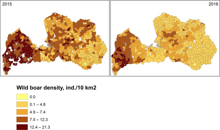
Wild boar population density in Latvia in 2015–2016, ind./10 km²

• Source: State Forest Service of Latvia

Figure C.3.

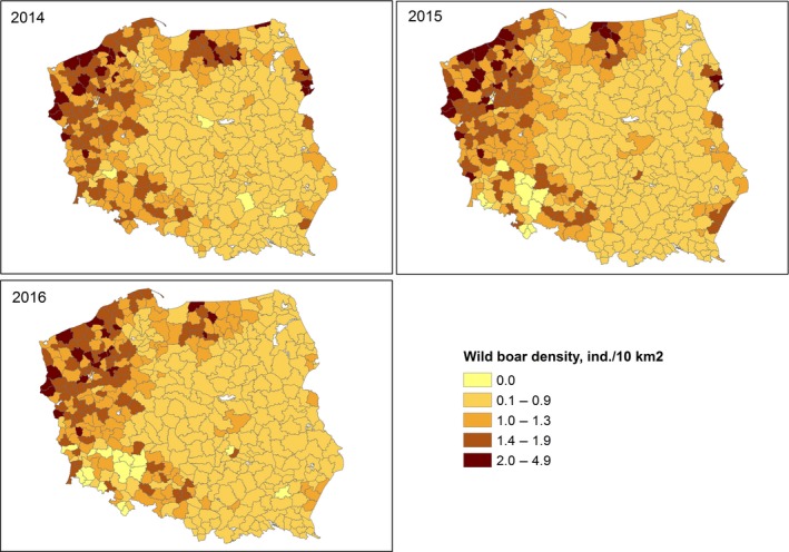
Estimated wild boar density in hunting rounds of Poland (2014–2016)

• Source: General Directorate of the State Forests (Poland)

Appendix D – Selective hunting of female wild boars and removal of dead animals

Table D.1.

Measures taking by the MS for wild boar management

	Selective hunting of female wild boars	Removal of dead animals	Additional feeding	Baiting	Driven hunts
Estonia	January 2016 From subadults and adults, 50% of wild boars shot must be females Decree of Environmental Board from 31.8.2016 Contracts with 124 hunting clubs/society	September 2014	Forbidden all year around September 2015	Max 100 kg in feeding machine, on ground max 5 kg of feed per feeding slot/place September 2015	Prohibited October 2014 Allowed September 2015
Latvia	November 2015	From June 2014	Banned since December 2014	Max 400 L per 1,000 ha only in containers ensuring dosage supply (dosimeter)	Allowed (except 20 km wide buffer zone in territories of Part 2 bordering Part 1)
Lithuania	November 2015	February 2016	Forbidden all year around	Max 100 kg in the specially designed content per baiting place. Forbidden to put the feed on the ground	Allowed from 15 October until 1 February
Poland	Included in the programme approved by the EU (implemented since 1 September 2016), concerns shooting of an adult female of a wild boar (adult meaning a wild boar, which carcass weighs at least 30 kg after removing the entrails). It covers all female wild boar (i.e. shot as a part of hunting plans and shot as a sanitary shooting) This measure is implemented on the area of WAMTA (see attached map) and within the areas defined in annex to the Commission Implementing Decision 2014/709/UE	Included in the programme approved by the EU (implemented since 1 September 2016). This measure is implemented on the area of WAMTA (see attached map) and within the areas defined in annex to the Commission Implementing Decision 2014/709/UE	Forbidden all year round within the areas defined in part II and III of the annex to the Commission Implementing Decision 2014/709/UE	Allowed in accordance with ASF Strategy for Eastern Part of the EU (the amount of feed is supposed not to exceed 10 kg/km2 per month)	Forbidden within the areas defined in part I, II and III of the annex to the Commission Implementing Decision 2014/709/UE

Appendix E – Classification of ASFV cases in wild boar populations depending on environmental and biological factors

Here, the focus is on discrimination techniques to classify regions with ASF cases from those that don't based on Classification and Regression Trees (Breiman et al., 1984). Classification and regression trees has been used for this purpose, following specific splitting rules, disjoint subsets of the data are constructed. These subsets are called nodes. Further splitting is repeated several times within these nodes. This partitioning process results in a saturated tree. The saturated binary tree (each node is splitted in two) is then pruned to an optimal size tree. This is the so‐called pruning process. The final step is the selection process, which determines the final tree.

The Partitioning Process

The partitioning process is based on splitting rules, which involve conditioning on predictor variables. The best possible variable to split the root node is the one that results in the most homogeneous and purest child nodes. A measure for the goodness of split is defined as the reduction in impurity. This partitioning process results in a saturated tree with the characteristic that if no limit is placed on the number of splits, eventually ‘pure’ classification will be achieved. In that case, the saturated tree is usually too large to be useful. Therefore, it is typically to set a minimum size of a node a priori or a maximum number of levels for the tree to reach (Breiman et al., 1984).

The Pruning Process

The point is to find the subtree of the saturated tree that is most predictive of the outcome and least vulnerable to noise in the data. Breiman et al. (1984) proposed to let the partitioning continue until the tree is saturated or nearly so, and this generally large tree is pruned from the bottom up using cost‐complexity method. Cost‐complexity pruning is defined as the cost (a measure for total impurity in the final nodes) for the tree plus a complexity parameter times the tree size.

The Selection Process

For the original data set, the cost decreases monotonically with increasing number of nodes. For the test data, the cost decreases with increasing number of nodes, but reaches a minimum and then increases as complexity increases. The optimal tree is that in which we obtain a minimum cost for the new data. Often, there are several trees with costs close to the minimum, then the smallest sized tree whose cost does not exceed the minimum cost plus the standard error of the cost will be chosen. The same procedure can be followed using k‐fold cross‐validation, in which k random subsamples, as equal in size as possible are formed from the learning sample. The classification tree of the specified size is computed k times, each time leaving out one of the subsamples from the computations, and using that subsample as a test sample for cross‐validation. The CV costs computed for each of the k test samples are then averaged to give the k‐fold estimate of the CV costs.

Handling Missing Data

One attractive feature of tree‐based methods is the ease with which missing values can be handled. There are several methods to deal with missing values. In this particular case, the used methods, uses the approach of surrogate splits, which attempt to utilise information in the other predictors to assist in making the decision to send an observation to the left or to the right daughter node. They look for the predictor that is most similar to the original predictor in classifying the observations. Similarity is measured by a measure of association. It is not unlikely that the predictor that yields the best surrogate split may also be missing. Then there will be looked for the second best, and so on. In this way, all available information is used.

Variable Importance Measure

The variable importance measure used was based on Breiman et al. (1984) proposal using the prune tree; the measure is computed as follow:

$$J_l^2(t)=\sum _{t=1}^{J-1}{\widehat{l}}_t^2·I(v(t)=l),$$

measuring the relevance for each predictor variable X _l. The sum is over the J − 1 internal nodes of the prune tree. At each such node t, five of the best input variables X _v(t) that could be used for partitioning the region associated with that node into two subregions; within each a separate constant is fit to the response values. The particular variables chosen are the ones that give maximal estimated improvement ${\widehat{l}}_t^2$ in squared error risk over that for a constant fit over the entire region. The squared relative importance of variable X _l is the sum of such squared improvements over all internal nodes for which it was chosen as the splitting variable.

Suggested citation: EFSA (European Food Safety Authority) , Cortiñas Abrahantes J, Gogin A, Richardson J and Gervelmeyer A, 2017. Scientific report on epidemiological analyses on African swine fever in the Baltic countries and Poland. EFSA Journal 2017;15(3):4732, 73 pp. doi: 10.2903/j.efsa.2017.4732

References

- Breiman L, 2001. Random forests. Machine Learning, 45, 5–32. [Google Scholar]
- Breiman L, Friedman JH, Olshen RA and Stone CJ, 1984. Classification and regression trees. Chapman and Hall, New York: 368 pp. [Google Scholar]
- EEA (European Environment Agency), 2007. CLC2006 technical guidelines. Technical report No 17/2007. ISSN 1725‐4012 2237, 66 pp.
- EFSA AHAW Panel (EFSA Panel on Animal Health and Welfare), 2015. Scientific opinion on African swine fever. EFSA Journal 2015;13(7):4163, 92 pp. doi: 10.2903/j.efsa.2015.4163 [DOI] [Google Scholar]
- FAO , 2013. African swine fever in the Russian Federation: risk factors for Europe and beyond. EMPRES WATCH, Vol. 28, May 2013. Rome.
- Lange M and Thulke HH, 2017. Elucidating transmission parameters of African swine fever through wild boar carcasses by combining spatio‐temporal notification data and agent‐based modelling. Stochastic Environmental Research and Risk Assessment, 31(2), 379–391. doi: 10.1007/s00477-016-1358-8 [DOI] [Google Scholar]
- Lunardon N, Menardi G and Torelli N. 2014. ROSE: A Package for Binary Imbalanced Learning. The R Journal (6/1). Available online: https://journal.r-project.org/archive/2014-1/menardi-lunardon-torelli.pdf
- Oļševskis E, Guberti V, Seržants M, Westergaard J, Gallardo C, Rodze I and Depner K, 2016. African swine fever virus introduction into the EU in 2014: experience of Latvia. Research in Veterinary Science, 105, 28–30. [DOI] [PubMed] [Google Scholar]
- Podgórski T, Lusseau D, Scandura M, Sönnichsen L and Jędrzejewska B, 2014. Long‐lasting, kin‐directed female interactions in a spatially structured wild boar social network. PLoS ONE, 11, e99875. doi: 10.1371/journal.pone.0099875 [DOI] [PMC free article] [PubMed] [Google Scholar]
- Riebler A, Sørbye SH, Simpson D and Rue H, 2016. An intuitive Bayesian spatial model for disease mapping that accounts for scaling. Statistical Methods in Medical Research 25, 1145–65. doi: 10.1177/0962280216660421 [DOI] [PubMed] [Google Scholar]
- Scholkopf B and Smola A, 2002. Learning with Kernels. MIT Press, Cambridge, MA, USA. [Google Scholar]
- SCPAFF (Standing Committee on Plants A, Food and Feed) 2016a. Presentation: ASF epidemiological situation in Latvia – 2016.
- SCPAFF (Standing Committee on Plants, Animals, Food and Feed), 2016b. SCPAFF, Brussels, 13.09.2016. Presentation: “Epidemiology of African swine fever in wild boar in Poland”. Available online: http://ec.europa.eu/food/committees/regulatory/scfcah/animal_health/docs/20140821_asf_lithuania_en.pdf
- Śmietanka K, Woźniakowski G, Kozak E, Niemczuk K, Frączyk M, Bocian Ł, Kowalczyk A and Pejsak Z, 2016. African swine fever epidemic, Poland, 2014–2015. Emerging Infectious Diseases, 22, 1201–1207. Available online: 10.3201/eid2207.151708 [DOI] [PMC free article] [PubMed] [Google Scholar]
- WAHIS (World Animal Health Information System), 2016. World Animal Health Information Database (WAHID) Interface from 1 July 2015 until 1 September 2016. Available online: http://www.oie.int/wahis_2/public/wahid.php/Wahidhome/Home