Adaptive Weighted Log Subtraction based on Neural Networks for Markerless Tumor Tracking using Dual-Energy Fluoroscopy

Abstract

Purpose:

To present a novel method, based on convolution neural networks (CNN), to automate weighted log subtraction (WLS) for dual-energy (DE) fluoroscopy to be used in conjunction with markerless tumor tracking (MTT).

Methods:

A CNN was developed to automate WLS (aWLS) of DE fluoroscopy to enhance soft tissue visibility. Briefly, this algorithm consists of two phases: training a CNN architecture to predict pixel-wise weighting factors followed by application of WLS subtraction to reduce anatomical noise. To train the CNN, a custom phantom was built consisting of aluminum (Al) and acrylic (PMMA) step wedges. Per-pixel ground truth weighting factors were calculated by minimizing the contrast of Al in the step wedge phantom to train the CNN. The pre-trained model was then utilized to predict pixel-wise weighting factors for use in WLS. For comparison, the weighting factor was manually determined in each projection (mWLS). The CIRS thorax phantom with five simulated spherical targets (5–25 mm) embedded in a lung-cavity, was utilized to assess aWLS performance. The phantom was imaged with fast-kV dual-energy (120 and 60 kVp) fluoroscopy using the on-board imager of a commercial linear accelerator. DE images were processed offline to produce soft-tissue images using both WLS methods. MTT was compared using soft-tissue images produced with both mWLS and aWLS techniques.

Results:

Qualitative evaluation demonstrated both methods achieved soft-tissue images with similar quality. The use of aWLS increased the number of tracked frames by 1–5% compared to mWLS, with the largest increase observed for the smallest simulated tumors. The tracking errors for both methods agreed within 0.1 mm.

Conclusions:

A novel method to perform automated WLS for DE fluoroscopy was developed. Having similar soft-tissue quality as well as bone suppression capability as mWLS, this method allows for real-time processing of DE images for MTT.

1. Introduction

Dual energy (DE) fluoroscopy involves obtaining continuous radiographic images at high (e.g. 120 kVp) and low (e.g. 60 kVp) x-ray tube energies^{1, 2}. By performing weighted logarithm subtraction (WLS) of the low energy from the logarithm of the high energy image, a third image is created that enhances soft-tissue visibility by reducing anatomical noise^{3, 4}. Using this technique, the weighting factor is optimized to selectively remove bone from the combined images^{1, 2, 4, 5}. Conventionally, the weighting factor is determined iteratively by minimizing the contrast between bone and neighboring soft-tissue regions^5–7. Although this approach works well for fixed-angle fluoroscopy, the weighting factor may require adjustments in radiotherapy applications where the gantry is rotating during image acquisition, such as for markerless tumor tracking (MTT)⁸ during treatments utilizing volumetric modulated arc therapy (VMAT) delivery. In these cases, the fraction of overlapping bone vs. soft tissue can change significantly from frame-to-frame⁸. Manual adjustment of the weighting factor limits the real time clinical applications of DE fluoroscopy for rotational acquisitions. Hence, a methodology that optimizes the weighting factors automatically for varying degrees of bone overlap and addresses the shortcomings of manual-WLS (mWLS) is required.

In this study, we describe an automated method, using neural networks, for optimizing the weighting factor on a pixel-by-pixel basis that addresses the previous limitations. The presented method consists of a calibration and inference phase. During the calibration phase a convolutional neural network (CNN) architecture is trained to identify the mapping between high/low energy fluoroscopy to the pixel-wise weighting factors. A phantom consisting of aluminum (Al) and acrylic (PMMA) step wedges is utilized for calibration where the corresponding pixel-wise weighting factors are determined by minimizing Al contrast. During the inference phase, the predicted weighting factors from the CNN are used to perform automated-WLS (aWLS). We validate this method using an anthropomorphic phantom and compare the results against the mWLS technique.

2. Material and Methods

2.1. Theory

DE imaging requires acquisition of two radiographic images at different x-ray tube potentials e.g., 120 kVp and 60 kVp⁹. At diagnostic x-ray energies, the Compton and photoelectric absorption dominate as photons interact with tissues in the body¹⁰. The Compton scattering cross-section is directly proportional to electron density and inversely proportional to incident photon energy (E_γ), while the photoelectric effect is proportional to atomic number (Z) and E_γ via Z³/E³_γ (up to 200 keV)¹⁰. Given these differences, Brody et al (1981) showed the possibility of combining two radiographic images so that one material (high or low Z) is subtracted¹. As an example of this technique, consider high (h) and low (l) mono-energetic photon beams irradiating a phantom composed of two homogeneous materials such as bone and soft tissue. The transmission intensity of each beam, as it strikes the imaging detector, is given by¹:

$$I_l= I_l^0\cdot e^{- {\mu }_l^{\mathit{\text{Soft}}} \cdot t_{\mathit{\text{Soft}}}- {\mu }_l^{\mathit{\text{Bone}}} \cdot t_{\mathit{\text{Bone}}}}$$ (1)

$$I_h= I_h^0\cdot e^{- {\mu }_h^{\mathit{\text{Soft}}} \cdot t_{\mathit{\text{Soft}}}- {\mu }_h^{\mathit{\text{Bone}}} \cdot t_{\mathit{\text{Bone}}}}$$ (2)

where μ and t represent the attenuation coefficient and thickness of each material, respectively. The intensities of individual pixels produced from the high and low energy images are given by I_h and I_l, respectively. In order to suppress bone, a weighted logarithmic subtraction of the two images can be performed, using following equation, which highlights soft tissue^{1, 9}:

$$DE=\text{ln}{I}_h-w_S\text{ln}{I}_l.$$ (3)

In the above equation ln and w_s are the natural logarithm and optimal weighting factor, respectively, required to produce the soft tissue image. Theoretically, in the limit when w_s approaches the ratio of linear attenuation coefficients of bone at high and low x-ray photons $\left(\frac{ {\mu }_h^{\mathit{\text{Bone}}}}{ {\mu }_l^{\mathit{\text{Bone}}}}\right)$, an optimal image is created that replaces the thickness of bone with tissue. However, clinical x-ray sources are polychromatic and varying thickness of the patient will affect beam hardening, resulting in different w_s values as the x-ray tube is rotated around the patient. Therefore, a computational method, described in Section 2.3, is required to select the optimal weighting factor.

2.2. Manual Weighting Factor Optimization (mWLS)

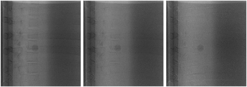
Conventionally, the weighting factor is optimized iteratively by reducing the contrast between regions of bone and neighboring soft-tissue^{5, 6}. Briefly, a 25×25 pixel region of interest (ROI) is placed in the bone and neighboring lung region of the phantom. The weighting factor w_s (in Equation 3) is then increased from 0 to 1 in increments of 0.01 to create DE images. For each weighting factor, the relative contrast between the bone and adjacent region is calculated in the resulting DE image. The optimal value of w_s is selected when the relative contrast is a minimum. Figure 1 shows DE images as the weighting factor is varied from 0.5 to 0.7 in 0.05 increments as well as the optimal weighting factor of 0.55 (top row last column). Of note, small variations in the weighting factor can result in less than complete subtraction of bone, and impact tumor visibility.

Figure 1.

Visualization of a 15 mm target overlapping with vertebrae as a function of the weighting factor. Starting at the top left, the weighting factors are 0.45, 0.5, 0.55, 0.6, 0.65 and 0.7 respectively. An optimal weighting factor is 0.55 shown on top row third column

In rotational acquisitions, the amount of bone in the pre-determined ROI may change significantly. This requires re-adjustment of the ROIs as well as optimization of weighting factors for each projection which can be laborious and time consuming process in clinical applications.

2.3. Automated Weighting Factor Optimization (aWLS)

To address the limitations of mWLS, an automated weight optimization methodology is developed that enables real-time removal of the bone with no further interaction. This novel technique is composed of three phases: determination of pixel-by-pixel true weighting factors, training a CNN architecture to map fluoroscopic projections into corresponding weighting factors and finally performing pixel-by-pixel WLS using predicted weights.

2.3.1. Calibration

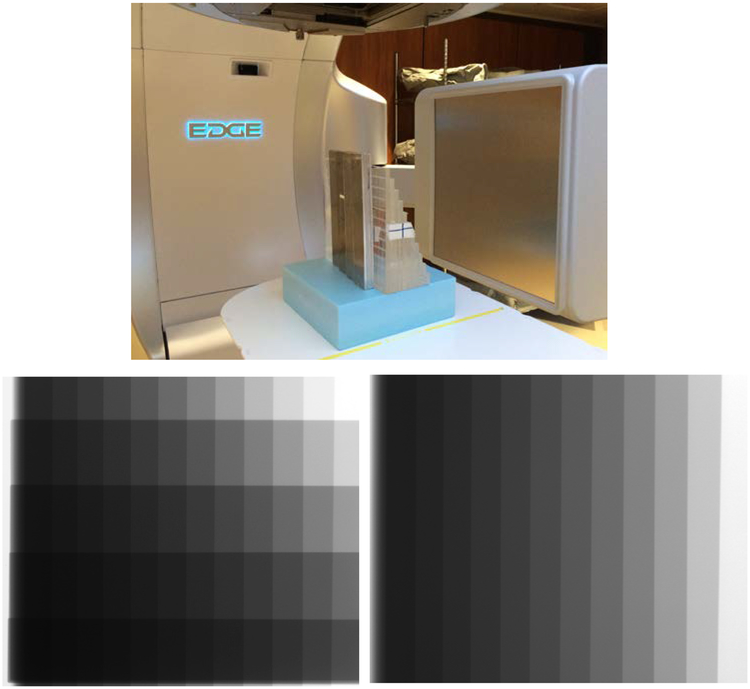
The soft tissue weighting factor is defined as the parameter that eliminates bone in the combined images and is determined by minimizing the relative contrast of the bone. To calibrate the weighting factors, a custom built wedge phantom consisting of various thicknesses of Al and PMMA was utilized. We use Al and PMMA as surrogates for bone and soft tissue due to their physical similarity and straightforward fabrication. The phantom consists 0.48 mm thick Al and 0.87 mm thick PMMA slabs that are stacked together to form step wedges with thicknesses varying between 0.48 to 1.92 cm and 0.87 to 9.57 cm, respectively (Figure 2, left). Two materials are then placed orthogonal to the direction of the x-ray beam to produce 60 different Al+PMMA thickness combinations (Figure 2, bottom left) using high (120 kVp, 15 mA, 20 ms) and low (60 kVp, 60 mA, 20 ms) x-ray tube settings.

Figure 2.

Demonstration of the calibration setup. The top image shows the wedge phantom on the treatment table in front of the OBI detector of the linac. A projection image of the of Al+PMMA phantom is shown in the lower left, while an image of the PMMA wedge alone is shown in the lower right.

To calculate the weighting factor for each pixel, the difference between the transmitted intensities of Al+PMMA and PMMA (background region) of DE image is minimized to yield an optimization problem stated as follows:

$${\text{min}}_{w_S\left(x.y\right)}\left|D{E}_{Al+\mathit{\text{PMMA}}}\left(w_S\right)- D{E}_{\mathit{\text{PMMA}}}\left(w_S\right)\right|.$$ (4)

Inserting Equation 3 as the minimization constraint and rearranging terms results in an equation that is described by raw measurements (the pixel dependency index is dropped in the subsequent discussion to avoid confusion of brackets):

$$\underset{w_S}{\text{min}}\left|\left(\text{ln}{I}_h^{Al+\mathit{\text{PMMA}}}- \text{ln}{I}_h^{\mathit{\text{PMMA}}}\right)- w_S* \left(\text{ln}{I}_l^{Al+\mathit{\text{PMMA}}}-\text{ln}{I}_l^{\mathit{\text{PMMA}}}\right)\right|.$$ (5)

In the mono-energetic approximation, Equation 5 can be further decomposed to the corresponding effective linear attenuation coefficients of the Al and PMMA:

$$\underset{ w_S}{\text{min}}\left|\left(-{\mu }_h^{Al}+ w_S* {\mu }_l^{Al}\right)*t_{Al}+ \left(-{\mu }_h^{\mathit{\text{PMMA}}}+ w_S* {\mu }_l^{\mathit{\text{PMMA}}}\right)*t_{\mathit{\text{PMMA}}}\right|.$$ (6)

Here, t_(Al,PMMA) and ${\mu }_{\left(h,l\right)}^{\left(Al,\mathit{\text{PMMA}}\right)}$ are thicknesses of Al or PMMA and effective linear attenuations of Al or PMMA at high/low energies, respectively. To produce the desired soft-tissue image, the first term in the parenthesis must vanish for all values of Al thickness (t_Al). Minimization of this equation is not trivial since there are ~10⁶ weighting factors that need to be optimized simultaneously within a typical image. However, instead of trying to minimize Equation 6, an alternative equation could be minimized to yield the same solution for the weighting factors:

$$\underset{ w_S}{\text{min}}\left|\left(-{\mu }_h^{Al}+ w_S* {\mu }_l^{Al}\right)*t_{Al}\right| = \underset{w_S}{\text{min}}\left|\left(\text{ln}{I}_h^{Al}- w_S*\text{ln}{I}_l^{Al}\right)\right|$$ (7)

It is important to emphasize that the solution for both Equation 6 and 7 are satisfied when the weighting factors (w_s) approach the ratio of the linear attenuation coefficients of Al at high and low energies ($\frac{{\mu }_h^{Al}}{{\mu }_l^{Al}}$). Equation 7 simplifies the minimization problem and can be solved

$$w_S=\frac{\text{ln}{I}_h^{Al} - \text{ln}{I}_h^0}{\text{ln}{I}_l^{Al} -\text{ ln}{I}_l^0} .$$ (8)

analytically using raw transmitted intensities by setting the minimum value to zero:

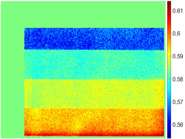
Here, $\text{ln}{I}_h^0$ and $\text{ln}{I}_l^0$ are the natural logarithm of air measurements at high and low energies, respectively, which are required for normalization. To suppress noise in the resulting weighting factors, a simple median smoothing filter with a kernel size of 11×11 is applied to the raw intensities before division. The weighting factor is undefined in air and soft-tissue only regions and was estimated using the average weighting factors of the remaining pixels. This last step is essential to train neural networks since patient images contain pixels without bone. Figure 3 depicts the weighting factors of the calibration phantom calculated as described above.

Figure 3.

Soft tissue weighting factor obtained using the wedge calibration phantom for each pixel. The edges of the phantom corresponding to air or PMMA are assigned average values. Each horizontal strip represents a different thickness of Al.

2.3.2. Training Phase

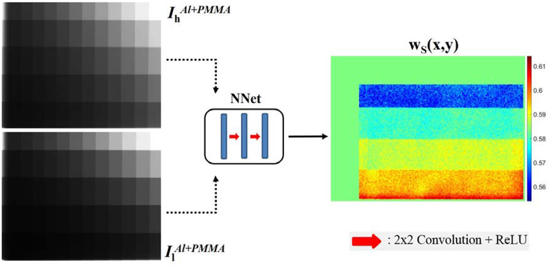
In the second step, the calibration phantom is utilized to train the neural network architecture that learns the mapping function between high/low Al+PMMA images to corresponding soft tissue weights using the full image resolution of 768×1024, as shown in Figure 4. The CNN architecture consists of three convolutional layers, each followed with linear rectifier (ReLU) activation. An intermediate 2×2 kernel size was selected to avoid any blurring effect. The number of filters in the first convolutional layer is 8 which was doubled in the following layers, totaling in 2746 trainable parameters. A shallow network was preferred without any down-sampling operation to emphasize mapping of the transmitted intensities to pixel weights rather than feature learning. The CNN architecture was implemented and trained using Keras neural networks API (v2.2.4)¹¹ with TensorFlow (v1.17)¹² engine on the backend.

Figure 4.

Flowchart of the training phase. Transmission intensity images (left), normalized to air, are passed into CNN architecture (middle) to predict corresponding weighting factors (right).

Prior to training, fluoroscopic images were normalized with the corresponding air intensities that were also acquired using same kVp settings, with the phantom and couch removed from the view. Next, the normalized images were linearized using the natural-logarithmic operation. This process is fundamental in training neural networks to eliminate scale variability of inputs (transmission intensities). The Stochastic Gradient Descent (SGD) algorithm with mini-batch size of 4, resulting in a 4×768×1024 tensor, was utilized to minimize the mean-squared error between the predicted and calculated weighting factors. Parameter optimization of CNN was performed using the Adam Optimizer¹³ with a learning rate of 0.001. In total 60 calibration phantom projections were utilized for training which were acquired using the high (120 kVp) and low (60 kVp) energy imaging protocol. To improve generalizability of the model, images were randomly shifted and rotated. Additionally, the CNN parameters were regularized using the L2 norm of 0.015 to reduce overfitting. Due to the relatively small learning rate, a total of 2000 training epochs was used. Performance of the CNN model was monitored on validation data and training terminated if no improvement was observed for 50 consecutive epochs. The training procedure was performed offline once and the trained model parameters were stored for future use.

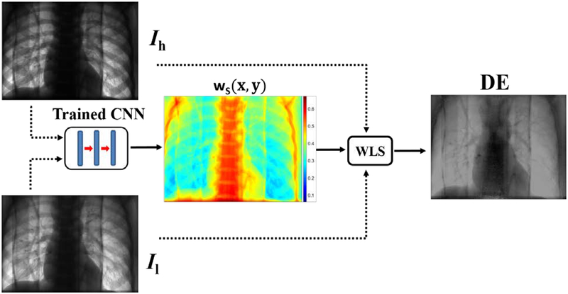
During inference, high-low images were used to predict weighting factors as a function of pixel location and were consequently used in WLS. This step occurs in real-time and eliminates the need for manual region selection and weight optimization. Figure 5 shows a flowchart of the aWLS method.

Figure 5.

Flowchart of the automated WLS method. I_h and I_l represents measured transmitted intensities of high and low kVp settings, respectively (left images). A mapping of the soft tissue weighting factors predicted using the pre-trained network is shown in the middle. The image on the right represents the DE image created by combining high and low energy images with the weighing factors using Equation 3.

2.4. Image Acquisition Using Fast-kVp Switching Dual-Energy Imager

DE images were acquired using fast-kV switching fluoroscopy implemented in Developer Mode of the TrueBeam linear accelerator ver 2.7MR3 (Varian Medical Systems, Palo Alto, CA). This approach enables rapid switching of the x-ray tube energy between programmed values. In this study, alternating 60 and 120 kVp x-rays were used based on a previous study by Haytmyradov et al.⁶ This study demonstrated that energy combinations of 140–60 kVp, 130–60 kVp and 120–60 kVp produced the highest (and statistically equivalent) signal-difference-to-noise ratios (SNDR) per unit dose. The mA setting for each pulse was adjusted to balance the air dose between the low (60 mA) and high (15 mA) kVp tube settings. The image acquisition rate was set to a maximum of 15 frames per second (fps). This rate results in DE images with an effective frame rate of 7.5 Hz. The source-to-axis distance (SAD) and source-to-image distance (SID) were 100 cm and 150 cm, respectively, and were fixed for all experiments. Acquired x-ray images were encoded in a 16 bit unsigned-integer having dimensions of 1024 × 768 and a pixel size of 0.388 mm (2×2 binned). These images were subsequently saved in the Varian proprietary XIM format. Following image acquisition, XIM files were processed with in-house software written in MATLAB (MathWorks, Natick, MA, USA) to create bone suppressed images using methods discussed in Section 2.2 and 2.3.

To evaluate aWLS, the CIRS dynamic thorax motion phantom (CIRS Inc. Norfolk, VA) was utilized. This phantom consists of tissue and lung-equivalent epoxy materials with a 3D anthropomorphic spine and ribs constructed from material that simulates cortical and trabecular bone. A motion controller is connected to the lung insert, and is capable of producing complex 3D motions by utilizing simultaneous translational and rotational movements with pre-programmed periodic waveforms. In this study, the cos⁴ waveform with peak-to-peak amplitude 15 mm and period of 2.5 sec was used to simulate respiratory motion in the inferior-superior direction. A soft tissue target insert was placed in a lung-equivalent compartment of the phantom to simulate tumor. Five different spherical target inserts with diameters of 5, 10, 15, 20 and 25 mm were used in this study. Separately, an anthropomorphic thorax phantom (Radiology Support Devices, Lung Chest Phantom, RS-315) was also utilized to perform qualitative assessment of images after WLS. Both the motion and the anthropomorphic phantoms were imaged in full 360 degree rotational acquisitions to validate robustness of WLS methods to varying degrees of bone-soft tissue overlap.

2.5. Motion Tracking

A non-commercial off-line research software (RapidTrack v3.0, Varian Medical Systems, Palo Alto, CA) was used for MTT¹⁴ in conjunction with the motion phantom. The MTT software is based on a template matching algorithm that localizes the position of the tumor in the radiographic image using templates derived from the computed tomography (CT) scan (Somatom Open AS, Siemens Healthineers, Germany). Templates were generated from a CT scan of the motion phantom and reconstructed with a 0.75 mm slice thickness. Contours of the individual targets were generated using Eclipse (ver 15.5, Varian). Subsequently, CT images and target contours were imported in the RapidTrack Planning v1.12 (Varian Medical Systems, Palo Alto, CA) to produce the individual templates.

Phantom DE fluoroscopy images were further processed using mWLS or aWLS methods to create soft-tissue images that were subsequently used with the templates to evaluate MTT. For each image, tracking was performed within a search window that was a 20 mm expansion of the template for each target. The template was scanned within the search window and at each location the normalized cross-correlation (NCC) was calculated producing a match score surface. The tracked location of the target was determined by the peak of the match score surface and the confidence in the match was obtained from the peak-to-side lobe ratio (PSR) of the surface¹⁵.

The method for obtaining ground truth (GT) locations of the target was described by Haytmyradov et al¹⁵. Subsequently, the distance between the tracked location and GT was determined for each tracking point. Values less than or equal to a defined threshold were tagged as true tracking events, while those values greater than the threshold were identified as false events. The threshold values were determined by computing the autocorrelation of each template with itself along with the width of the autocorrelation peak. The resultant thresholds were 1.3, 2.1, 2.5, 3.3, and 3.5 mm for the 5, 10, 15, 20 and 25 mm targets, respectively. In this analysis, PSR was used as a discriminator. Tracking accuracy was calculated as the difference between tracked locations and the ground truth of simulated tumors.

3. Results

4.1. Weighting factors

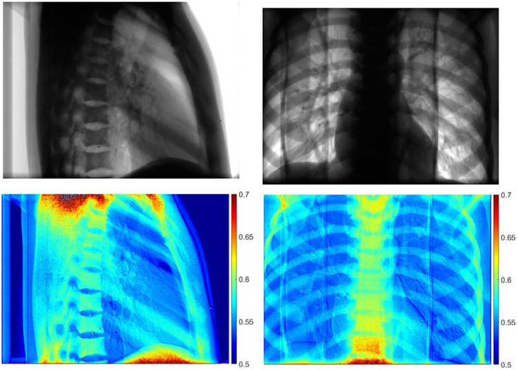
Due to the large number of frames, mWLS was applied every 20 frames and then forward projected for the next frames⁸. Depending on the gantry angle, the weighting factors varied from 0.54 to 0.61 using mWLS method, where a single weighting factor is used per projection. The aWLS method, however, is granular and the weights are determined for each pixel in every projection. Two examples of the aWLS weighting factors are shown in Figure 6 with the corresponding 60 kVp image (shown on top row). Predicted weighting factors change with the amount of bone overlap and larger values are observed in regions containing thicker amounts of bone such as the spine.

Figure 6.

Demonstration of weighting factors obtained using neural networks. Projections of the anthropomorphic phantom at 60 kVp (top) and corresponding pixel-wise weighting factors for two different views. Higher values of the weighting factor are observed for bone pixels. The shoulder and abdominal region has higher values due to photon starvation.

Qualitative Evaluation

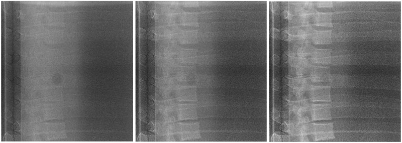
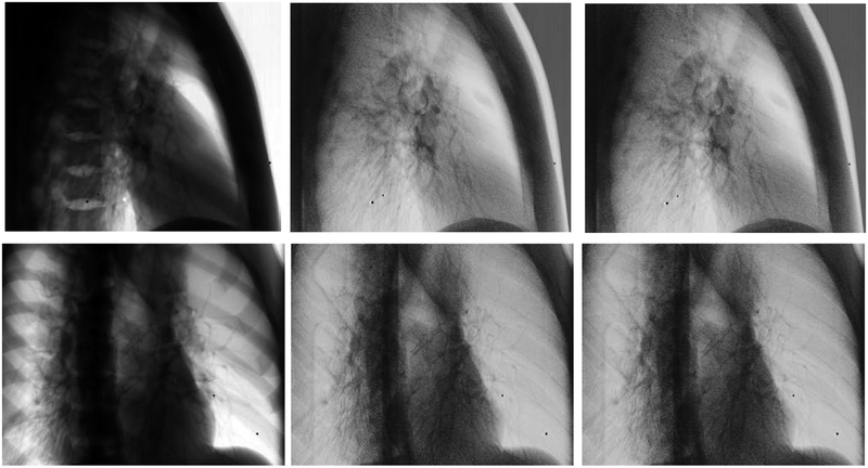
To qualitatively assess bone suppression capability of the WLS methods, several projections consisting of various amounts of bone and soft-tissue overlaps were compared side-by-side. For the CIRS phantom, a 25 mm tumor inserted in the lung cavity of the phantom was compared against single (120 kVp) and DE images obtained with both WLS methods. Results of this comparison are shown in Figure 7. Similarly, the anthropomorphic thorax phantom was imaged at two different gantry angles corresponding to the largest amount of bone and soft-tissue overlap (Figure 8). Both DE images reduced anatomical noise and improved visibility of soft-tissue. Moreover, no apparent visual differences were observed in the resulting DE images with aWLS vs. mWLS.

Figure 7.

Projections of the CIRS phantom using 120kVp (left column), mWLS (middle column) and aWLS (right column) at 270 gantry angle. No expressive differences are observed between mWLS and aWLS techniques.

Figure 8.

Projections of the anthropomorphic thorax phantom using 120 kVp (left column), mWLS (middle column) and aWLS (right column) imaging at 270 and 315 gantry angles. No visual differences are observed between the both WLS techniques. Note: this phantom does not have an embeded tumor in the lung.

4.3. Tracking Evaluation

The MTT results are summarized in Table 1. The PSR threshold is shown for both methods as a function of target size. This value represents the PSR value required to maintain a false tracking event rate of < 0.05. In general, the PSR thresholds were slightly lower for aWLS vs. mWLS across nearly all target sizes. As such, aWLS resulted in a higher percentage of frames for which tracking was accurately performed. The average PSR values as a function of target size were slightly less with aWLS vs. mWLS due to the lower PSR threshold with the maximum difference in average PSR of 0.18 observed for the 25 mm target. The effect of these two methods on local accuracy showed differences of < 0.1 mm across all tumor sizes, which were not statistically significant. In sum, both aWLS and mWLS produced nearly equivalent tracking results with a slight advantage to the aWLS method as it increased number of successfully tracked frames, particularly for smaller targets.

Table 1.

MTT comparison between aWLS and mWLS methods. Each column represents simulated tumor diameter. Tracking local accuracy is similar using both methods, while tracking success rate is slightly improved with the aWLS method.

	PSR Threshold
Target Size	5 mm	10 mm	15 mm	20 mm	25 mm
aWLS	3.08	3.67	3.80	3.68	3.28
mWLS	3.15	3.72	3.84	3.68	3.78
	Tracked Frames
Target Size	5 mm	10 mm	15 mm	20 mm	25 mm
aWLS	239/438 (54.5%)	367/446 (82.3%)	386/446 (86.5%)	428/448 (95.5%)	444/447 (99.3%)
mWLS	216/438 (49.3%)	350/446 (78.5%)	377/446 (84.5%)	411/448 (91.7%)	441/447 (98.7%)
p-value	<0.01	<0.01	<0.01	<0.01	<0.01
	Mean PSR (Std. Dev) Values
Target Size	5 mm	10 mm	15 mm	20 mm	25 mm
aWLS	3.42+/−0.22	4.76+/−0.52	5.64+/−0.91	6.08+/−1.22	6.67+/−1.29
mWLS	3.47+/−0.22	4.85+/−0.50	5.71+/−0.92	6.22+/−1.26	6.85+/−1.25
p-value	0.02	0.02	0.29	0.10	0.04
	Tracking Accuracy (mm)
Target Size	5 mm	10 mm	15 mm	20 mm	25 mm
aWLS	2.74 ± 4.82	0.89 ± 2.37	0.51 ± 1.61	0.38 ± 0.69	0.31 ± 0.28
mWLS	2.83 ± 4.99	0.85 ± 2.38	0.59 ± 2.12	0.38 ± 0.50	0.30 ± 0.51
p-value	0.79	0.8	0.53	1.0	0.72

4. Discussion

The WLS technique used in conjunction with DE imaging has been shown to improve tumor localization^{5, 16–18} and enhance performance of MTT methods^{4, 8, 19–21} by suppressing bony anatomy. Conventionally, soft-tissue images are created by reducing the contrast of the bone and neighboring soft-tissue region followed by assigning a global weighting factor across the image. Although, this method shows promising results, its application is limited to static projections. Moreover, a global weighting factor may not be ideal to completely eliminate bones due to variations of densities and thicknesses of materials within the body.

Darvish-Molla et al. (2019) proposed an algorithm to calculate pixel-based weighting factors using prior CT data²². Their algorithm consists of pre-calculating weighting factors using a calibration phantom. Next, a CT image of the phantom is used to create digitally reconstructed thicknesses (DRTs) of bone and soft-tissue. To determine pixel-wise weighting factors, the weighting values for different pixel locations are determined by interpolating (or extrapolating) the values of the pre-calculated weighting factors. Comparisons of measured and simulated weighting factors demonstrated 3% agreement for all bone overlap regions. One disadvantage of this method is that the calculated pixel-wise weights may be misaligned with real-time projections and hence accurate image registration is necessary to produce high quality subtraction.

In our study, a novel method was developed to automate WLS of DE imaging based on neural networks. As described previously, the algorithm consists of creating per-pixel weighting factors using a calibration phantom and training a neural network that maps projections of the calibration phantom at high/low photon energies to corresponding weighting factors. During the inference, the pre-trained model is used to predict weighting factors for a given phantom and perform WLS to remove bones. In this study, a step wedge phantom was used for calibration purposes. However, the methodology described herein is not limited to a particular calibration phantom. In particular, utilization of ramp phantom would provide larger dynamic range for Al+PMMA thickness combinations. Additionally, our method uses raw projections for both the weighting factor calculation and subsequently WLS, thus eliminating misregistration issues. In this study, the CNN architecture was preferred to map transmission intensities to weighting factors, however, other machine learning strategies such as polynomial regression can also be employed²³. One limitation of this study is that Al and PMMA were used as a surrogate for bone and soft tissues. However, the impact of this approximation on the resultant images and MTT is minimal.

Deployment of the presented methodology follows the natural workflow of clinical image acquisition. To create soft-tissue images from DE images, the pre-trained model can be stored and used to perform WLS in real-time. The model can be verified and/or re-calibrated during routine quality assurance following the methodology described above.

5. Conclusion

A novel method to automate WLS of DE imaging was developed to adaptively determine per-pixel weighting factors and create soft-tissue images. The presented method was validated both qualitatively and quantitatively by comparing to aWLS to mWLS. Results of this study showed that visually aWLS is similar to mWLS, while in terms of tumor MTT, aWLS had a slight advantage over mWLS. The developed aWLS method is fully automated allowing for real-time processing of DE images in clinical applications. By providing real-time visualization of lung tumors, DE imaging using the OBI on a linac can enhance MTT and image-guided radiotherapy.

References

- 1.Brody WR, Butt G, Hall A, and Macovski A, A method for selective tissue and bone visualization using dual energy scanned projection radiography, Med. Phys 8(3), 353–357 (1981). [DOI] [PubMed] [Google Scholar]
- 2.Shkumat NA, Siewerdsen JH, Richard S, Paul NS, Yorkston J, and Van Metter R, Dual-energy imaging of the chest: Optimization of image acquisition techniques for the “bone-only” image, Med. Phys 35(2), 629–632 (2008). [DOI] [PubMed] [Google Scholar]
- 3.Block AM, Patel R, Panfil J, et al. , Evaluation of a Template-Based Algorithm for Markerless Lung Tumor Tracking on Single Energy and Dual Energy kV Images, Int. J. Radiat. Oncol 90(1), S142–S143 (2014). [Google Scholar]
- 4.Patel R, Panfil J, Campana M, et al. , Markerless motion tracking of lung tumors using dual-energy fluoroscopy, Med. Phys 42(1), 254–262 (2015). [DOI] [PubMed] [Google Scholar]
- 5.Hoggarth MA, Luce J, Syeda F, et al. , Dual energy imaging using a clinical on-board imaging system, Phys. Med. Biol 58(12), 4331–4340 (2013). [DOI] [PubMed] [Google Scholar]
- 6.Haytmyradov M, Patel R, Mostafavi H, et al. , A novel phantom for characterization of dual energy imaging using an on-board imaging system, Phys. Med. Biol 64(3), 03NT01 (2019). [DOI] [PMC free article] [PubMed] [Google Scholar]
- 7.Yang Y, Zhong Z, Guo X, et al. , A Novel Markerless Technique to Evaluate Daily Lung Tumor Motion Based on Conventional Cone-Beam CT Projection Data, Int. J. Radiat. Oncol 82(5), e749–e756 (2012). [DOI] [PubMed] [Google Scholar]
- 8.Haytmyradov M, Mostafavi H, Wang A, et al. , Markerless Tumor Tracking using Fast‐ kV Switching Dual Energy Fluoroscopy on a Benchtop System, Med. Phys. mp 13573 (2019). [DOI] [PMC free article] [PubMed] [Google Scholar]
- 9.Bushberg JT, Seibert AJ, Leidholdt EM, and Boone JM, The Essential Physics of Medical Imaging, Third Edit (Lippincott Williams & Wilkins, Philadelphia, 2011). [Google Scholar]
- 10.Hubbell J and Seltzer S, Tables of X-Ray Mass Attenuation Coefficients and Mass Energy-Absorption Coefficients (version 1.4), (2004).
- 11.Chollet F, Keras API, (2015).
- 12.Martín Abadi EB, Agarwal Ashish, Barham Paul, Chen A.D. Zhifeng, Citro Craig, Corrado Greg S., Dean I.G. Jeffrey, Devin Matthieu, Ghemawat Sanjay, et al. , TensorFlow: Large-Scale Machine Learning on Heterogeneous Systems, (2015).
- 13.Kingma DP and Ba J, Adam: A Method for Stochastic Optimization, (2014).
- 14.Mostafavi H, Sloutsky A, and Jeung A, Detection and localization of radiotherapy targets by template matching, in 2012 Annu. Int. Conf. IEEE Eng. Med. Biol. Soc(IEEE, 2012), pp. 6023–6027. [DOI] [PubMed] [Google Scholar]
- 15.Haytmyradov M, Mostafavi H, Wang A, et al. , Markerless tumor tracking using fast-kV dual energy fluoroscopy of a benchtop system, Med. Phys In Press (n.d.). [DOI] [PMC free article] [PubMed] [Google Scholar]
- 16.Sherertz T, Hoggarth M, Luce J, et al. , Prospective evaluation of dual-energy imaging in patients undergoing image guided radiation therapy for lung cancer: Initial clinical results, Int. J. Radiat. Oncol. Biol. Phys 89(3), 525–531 (2014). [DOI] [PubMed] [Google Scholar]
- 17.Szucs-Farkas Z, Patak MA, Yuksel-Hatz S, Ruder T, and Vock P, Single-exposure dual-energy subtraction chest radiography: Detection of pulmonary nodules and masses in clinical practice, Eur. Radiol 18(1), 24–31 (2008). [DOI] [PubMed] [Google Scholar]
- 18.Fischbach F, Freund T, Röttgen R, Engert U, Felix R, and Ricke J, Dual-Energy Chest Radiography with a Flat-Panel Digital Detector: Revealing Calcified Chest Abnormalities, Am. J. Roentgenol 181(6), 1519–1524 (2003). [DOI] [PubMed] [Google Scholar]
- 19.Block AM, Patel R, Surucu M, Harkenrider MM, and Roeske JC, Evaluation of a template-based algorithm for markerless lung tumour localization on single- and dual-energy kilovoltage images, Br. J. Radiol 89(1068), 20160648 (2016). [DOI] [PMC free article] [PubMed] [Google Scholar]
- 20.Menten MJ, Fast MF, Nill S, and Oelfke U, Using dual-energy x-ray imaging to enhance automated lung tumor tracking during real-time adaptive radiotherapy, Med. Phys 42(12), 6987–6998 (2015). [DOI] [PubMed] [Google Scholar]
- 21.Dhont J, Verellen D, Poels K, et al. , Feasibility of markerless tumor tracking by sequential dual-energy fluoroscopy on a clinical tumor tracking system, Radiother. Oncol 117(3), 487–490 (2015). [DOI] [PubMed] [Google Scholar]
- 22.Darvish-Molla S, Reno MC, and Sattarivand M, Patient-specific pixel-based weighting factor dual-energy x-ray imaging system using a priori CT data, Med. Phys 46(2), 528–543 (2019). [DOI] [PubMed] [Google Scholar]
- 23.Gergonne J, The application of the method of least squares to the interpolation of sequences, Hist. Math 1(4), 439–447 (1974). [Google Scholar]