A geometric diffuse-interface method for droplet spreading

Abstract

This paper exploits the theory of geometric gradient flows to introduce an alternative regularization of the thin-film equation valid in the case of large-scale droplet spreading—the geometric diffuse-interface method. The method possesses some advantages when compared with the existing models of droplet spreading, namely the slip model, the precursor-film method and the diffuse-interface model. These advantages are discussed and a case is made for using the geometric diffuse-interface method for the purpose of numerical simulations. The mathematical solutions of the geometric diffuse interface method are explored via such numerical simulations for the simple and well-studied case of large-scale droplet spreading for a perfectly wetting fluid—we demonstrate that the new method reproduces Tanner’s Law of droplet spreading via a simple and robust computational method, at a low computational cost. We discuss potential avenues for extending the method beyond the simple case of perfectly wetting fluids.

1. Introduction

This work is concerned with the thin-film equation

$$\frac{\mathrm{\partial }h}{\mathrm{\partial }t}=-\frac{\mathrm{\partial }}{\mathrm{\partial }x}\left(h^n\frac{{\mathrm{\partial }}^{3}h}{\mathrm{\partial }{x}^3}\right),t>0,\hspace{0.17em}x\in (-\mathrm{\infty },\mathrm{\infty }),$$ 1.1a

and

$$h(x,t=0)=h_0(x),h_0(x)\ge 0,\hspace{0.17em}x\in (-\mathrm{\infty },\mathrm{\infty }),$$ 1.1b

and its modifications. Boundary conditions are chosen as |x| → ∞, so that equation (1.1) conserves mass:

$$\frac{\mathrm{d}M}{\mathrm{d}t}=0,M={\int }_{-\mathrm{\infty }}^{\mathrm{\infty }}h(x,t)\hspace{0.17em}\mathrm{d}x.$$ 1.2

The particular value n = 3 is physically relevant, as then equation (1.1) is a model for the free surface of a viscous thin-film flow. Indeed, equation (1.1) with n = 3 amounts to the Navier–Stokes equations for a thin-film flow, in the limit of lubrication theory. The derivation can be found in [1,2]. A sketch of the physical scenario is given in figure 1. The case n = 3 is the subject of the present article. In particular, we revisit the problem of droplet spreading, that is, we seek to model the time evolution of an initial profile h₀(x) with compact support.

Figure 1.

Schematic description of the fluid mechanical problem of droplet spreading, as derived from the Navier–Stokes equations in the lubrication limit. (Online version in colour.)

For a general value of n, the spreading of droplets governed by equation (1.1) admits the similarity solution [3]

$$h(x,t)=t^{-a}f\left(\frac{x}{t^a}\right),a=\frac{1}{n+4}.$$ 1.3

Substituting this trial solution into equation (1.1) yields the ordinary differential equation

$$f^n{f}^{‴}=\frac{\eta f}{n+4}.$$ 1.4

For n < 3, equation (1.4) possesses smooth solutions with compact support. In this case, equation (1.4) with initial conditions f(0) = 1, f′(0) = 0 and f″(0) = −μ < 0 can be solved by adjusting μ until f = f′ = 0 at some η = η₀ > 0, corresponding to the outermost extent of the droplet. Thus, the position x₀ of the microscopic contact line where the free surface h(x, t) touches down to zero is described by x₀ = η₀ t^1/(n+4). Unfortunately, this description breaks down precisely for the physically relevant value of n = 3, at which f(η) degenerates into a Dirac delta function centred at η = 0, and the droplet does not spread [4].

Physically, the breakdown of equation (1.1) as a model of droplet spreading for n = 3 is due to a small but not ignorable effect which occurs in the vicinity of the microscopic contact line. Namely, the modelling assumptions that enable the passage from the Navier–Stokes equations for a thin film to the simplified free-surface evolution equation (1.1) assume there is no relative motion between the film and the underlying substrate. (This is the no-slip condition.) However, the no-slip condition is not consistent with a moving contact line. Many different approaches have been proposed in the literature to restore the missing physics. Three of these approaches will be summarized below. These approaches all exhibit the same qualitative behaviour. However, they each have certain drawbacks. The short summaries of the three main approaches given below will provide the context in which our own proposal for healing the contact-line singularity will be introduced.

(a). Slip-length modelling

A common approach in the modelling literature to resolving the paradox of the moving contact-line is to modify equation (1.1) (with n = 3) as follows,

$$\frac{\mathrm{\partial }h}{\mathrm{\partial }t}=-\frac{\mathrm{\partial }}{\mathrm{\partial }x}[(h^3+\mathrm{\lambda }{h}^2)\frac{{\mathrm{\partial }}^{3}h}{\mathrm{\partial }{x}^3}],t>0,x\in (-\mathrm{\infty },\mathrm{\infty }),$$ 1.5

where λ is a positive (dimensionless) constant related to the slip length. Equation (1.5) can be derived using lubrication theory, starting from the Navier–Stokes equations. Instead of imposing the no-slip condition on the velocity component u(x, y = 0, t) tangent to the substrate, one instead imposes the condition

$$u(x,y=0,t)={\mathrm{\lambda }}_{\ast }{\left(\frac{\mathrm{\partial }u}{\mathrm{\partial }y}\right)}_{y=0},$$ 1.6

where ${\mathrm{\lambda }}_{\ast }$ is the dimensional slip length. Working in the limit of lubrication theory, and using appropriate non-dimensionalization, one obtains equation (1.5) in this manner.

Typically, one works with λ ≪ 1, as the effect of slip is a small but not ignorable. Then, equation (1.5) can be solved via the method of matched asymptotic expansions [5]. In this approach, one distinguishes between inner and outer solutions, separated by a lengthscale x_m(t), which demarcates the regions of validity of the different solutions. The geometry of this set-up is shown in figure 2. In the outer region, with |x| ≪ x_m(t), the effect of slip is ignorable, and one can work with λ = 0 in equation (1.5). The free-surface profile in this outer region can therefore be well approximated by the similarity solution (1.4) with n = 3. By not continuing this solution past |x| = x_m, the singularity that occurs in the similarity solution is avoided.

Figure 2.

Schematic description of the fluid mechanical problem of droplet spreading, showing the inner and outer regions of the problem. (Online version in colour.)

In the inner region, we identify the microscopic contact line x = x₀(t) where the free-surface height touches down to zero in a smooth fashion, h(x₀, t) = 0 and h_x(x₀, t) = 0. As such, the inner region corresponds to |x − x₀| ≪ λ. In this region, one therefore solves equation (1.5) without the h³ term. It is the disappearance of the h³ term in this limit which enables the smooth touchdown of the solution at x = x₀(t). Finally, the inner and outer solutions are matched at the scale x_m. As such, the position x_m is interpreted as the macroscopic contact line, and tanθ_m = h_x(x_m, t) has the interpretation of the macroscopic contact angle. Correspondingly, the position x₀ has the interpretation of the microscopic contact line, meaning that the microscopic contact angle tanθ₀ = h_x(x₀, t) is zero. It can be noted that this description deals with perfect wetting, such that the droplet spreads indefinitely, and the macroscopic contact angle tends to zero as t → ∞. For simplicity, we restrict our attention in the present article to this particular case (perfect wetting, zero equilibrium macroscopic contact angle), although extensions to partial wetting and finite equilibrium macroscopic contact angle are anticipated in future works.

The working-out of the matched asymptotic expansion procedure requires many intermediate steps before the final answer is obtained. These steps are summarized in [6], while the authors in [7–10] provide additional insights into the importance of the ordering of the capillary number and the slip length for the perturbation expansions and the resulting matching of the inner and outer solutions. The result of this procedure can be summarized in the following relation for the macroscopic contact angle (up to prefactors):

$${\left(\frac{\mathrm{\partial }h}{\mathrm{\partial }x}\right)}_{x=x_{\text{m}}}^3\sim \left(\frac{\mathrm{d}{x}_{\text{m}}}{\mathrm{d}t}\right)\ln \left[\frac{x_{\text{m}}}{\mathrm{\lambda }b}{\left(\frac{\mathrm{d}{x}_{\text{m}}}{\mathrm{d}t}\right)}^{1/3}\right],$$ 1.7

where b is a constant [6]. Equation (1.7) was also discovered via a different approach in Voinov [11]. Upon identifying the outer solution on the left-hand side of equation (1.7) with the similarity solution (1.3) h = t^−ah(x/t^a) with a = 1/7, equation (1.7) reduces to

$$\left(\frac{\mathrm{d}{x}_{\text{m}}}{\mathrm{d}t}\right)t^{6/7}=\text{const.}+\text{Logarithmic corrections},$$

hence, the leading-order behaviour of equation (1.7) is given by x_m ∼ t^1/7, which is the experimentally validated Tanner’s Law [1,12], valid for a droplet spreading of a perfectly wetting fluid. As such, the leading-order behaviour of the Navier slip model is consistent with experimental findings.

Although the Navier slip model (1.6) alleviates the singularity in the free-surface height h(x, t) at the microscopic contact line, the higher spatial derivatives of h(x, t) remain singular there. This means the capillary pressure P = −h_xx is singular at the microscopic contact line. Although the resulting singularity is rather mild, it does correspond to infinite pressure, which is undesirable in a physical model (although the integral of the pressure, or the force, does remain finite). Also, the prescription of the slip model (1.6), while convenient from the modelling point of view, does not have an a priori theoretical basis, beyond the obvious connection to atomic-scale fluid–substrate interactions. These two drawbacks have motivated the development of other models of droplet spreading.

(b). Precursor-film modelling

Here, a potential function Φ(h) is introduced which governs the molecular interactions between the fluid particles and the substrate. The choice of Φ(h) is dictated by the physics of the fluid–substrate interaction [13,14]. In the lubrication limit, the result of this modelling step is again a single equation for the droplet profile h(x, t); instead of h_t = −∂_x(h³∂_x P) with P = −h_xx one has

$$\frac{\mathrm{\partial }h}{\mathrm{\partial }t}=-\frac{\mathrm{\partial }}{\mathrm{\partial }x}\left(h^3\frac{\mathrm{\partial }P}{\mathrm{\partial }x}\right),P=-\frac{{\mathrm{\partial }}^{2}h}{\mathrm{\partial }{x}^2}+\mathit{\Phi }(h),$$ 1.8

where Φ is fluid–substrate interaction potential. This description gives a solution for h(x, t) which allows for droplet spreading.

The model (1.8) can be used to describe droplet spreading with zero macroscopic equilibrium contact angle, as well as finite macroscopic equilibrium contact angle. For the case of zero macroscopic equilibrium contact angle, de Gennes [13] has shown that droplet solutions of equation (1.8) possesses a precursor film—an ultra-thin film that persists beyond the droplet core. The structure of the precursor film can be quite complicated and depends in detail on the interaction potential Φ(h). For suitable functional forms of the interaction potential Φ(h), equation (1.8) also admits solutions corresponding to a finite macroscopic equilibrium contact angle. A further advantage of the model is the droplet-spreading solution maintains a finite stress at the contact line—and yet the leading-order behaviour of the precursor-film and Navier-slip models agrees, in a theory of matched asymptotic expansions [15].

In numerical simulations, the detailed structure of the precursor film is often neglected, it is simply set to be a uniform film that extends indefinitely beyond the droplet core. This modelling approach may be undesirable in multiphase flow applications—for instance, in drop deposition on a substrate, where the substrate should properly be assumed to be initially free from contamination by the fluid phase. The development of the present geometric diffuse-interface method is an attempt to address this problem.

(c). Diffuse-interface modelling

We summarize the diffuse-interface model in the context of the full Navier–Stokes equations, from which the thin-film equation (1.1) emerges as a limit. In the full Navier–Stokes equations, the motion of a droplet over a wall can be modelled using such a method. In addition to the velocity and pressure fields, an auxiliary order-parameter variable C (the ‘phase field’) is introduced, which tracks the phases, such that C = 1 inside the droplet and C = 0 outside, in the surrounding phase. There is a smooth transition between these two extreme values across a finite width—hence, a diffuse interface. The phase field evolves according to its own evolution equation, which is typically taken as the Cahn–Hilliard equation [16], thereby resulting in a mathematically consistent framework. By introducing the diffuse interface in this manner (rather than having a sharp interface at the contact line), the model effectively produces slip, through the diffusive fluxes. Hence, the stress singularity at the moving contact line is removed even when a no-slip velocity boundary condition is imposed [17,18].

In this work, we propose a regularization of equation (1.1) in the spirit of the diffuse–interface method. As such, we propose a modified version of equation (1.1) which depends not only on the free-surface height h(x, t) but also on a diffuse free-surface height,

$$\overline{h}(x,t)={\int }_{-\mathrm{\infty }}^{\mathrm{\infty }}K(x-y;\alpha )h(y,t)\hspace{0.17em}\mathrm{d}y:=K\ast h,$$ 1.9

where K(s;α) is a smoothing kernel which smooths out small-scale features on a lengthscale α or less. The regularization is not ad-hoc, instead, it is introduced in the context of a rigorous gradient-energy theory in §2. The proposed regularization method has some advantages over the other methods considered herein, in particular:

• —In contrast to the slip model, the proposed regularization produces a continuous pressure profile everywhere. We demonstrate below that our new theoretical model amounts to imposing the usual fluid-mechanical interfacial conditions on the filtered free-surface height $\overline{h}$, rather than on h. In a context where the free surface h comes into contact with a substrate which has some atomic level of roughness, this makes physical sense, and the use of $\overline{h}$ reflects our uncertain knowledge of the precise location where the droplet, the surrounding medium, and the substrate all come into contact. The parameter α can therefore be viewed as expressing this uncertainty.
• —In contrast to the precursor-film method, we do not require a precursor film of small-but-finite thickness to extend to infinity. Our model effectively has a precursor film whose thickness falls off to zero at large distances from the droplet core, the falloff scale is exactly α.
• —Although motivated by the diffuse-interface concept, our model does not dispense with the classical description of a sharp interface separating the fluid phases. As such, the sharp interface is still contained in our model; although it is no longer a dynamic variable, and it is recovered from what is effectively a diffuse interface via a deconvolution operation (cf. equation (1.9)).

By now one may have recognized that each of the above canonical methods involves a small length scale, as summarized in table 1. Therefore, it can be seen that each of the methods is concerned effectively with parametrization missing the small-scale physics, to produce the same large-scale droplet-spreading dynamics in each case. Our model also fits into this framework, as shown in table 1. We will further illustrate this and other features of our model by using numerical simulations in §3.

Table 1.

Summary of the various small length scales used in the different regularization methods.

method	lengthscale
Navier slip model	slip length
attractive/repulsive potential	precursor-film thickness
diffuse-interface method	diffuse-interface thickness
the present method	length scale of smoothing kernel

We conclude this Introduction by noticing that the standard thin-film equation (1.1), the thin-film equation with the precursor film (1.8), and the thin-film equation in the geometric diffuse-interface formulation (§2) all possess a gradient-flow structure, which means they can be associated with a certain energy functional E[h], such that the corresponding evolution equation can be written as h_t = −∂_x[Q∂_x (δE/δh)], where Q is a mobility function. This more general formulation brings the various thin-film equations into a generic class of models (for conserved fields) which include the Cahn–Hilliard equation [19,20], models for molecular beam epitaxy [21], models of phase-field crystals [20], other models for contact-line motion [22], as well as thin-film models wherein the free-surface height is coupled to scalar order parameters [23,24]. Therefore, insights gained by studying the equations arising from geometric diffuse interface method equations may apply more broadly. This observation places the proposed methodology into a wider context of physical applications.

(2). Theoretical analysis

The starting-point of the theoretical analysis is to notice that under the dynamics of equation (1.1), the following free-energy functional decays with time:

$$E=\frac{1}{2}{\int }_{-\mathrm{\infty }}^{\mathrm{\infty }}|{\mathrm{\partial }}_{x}h{|}^2\hspace{0.17em}\mathrm{d}x.$$ 2.1

Indeed, since δE/δh = −∂_xxh, equation (1.1) can be re-written as

$$\frac{\mathrm{\partial }h}{\mathrm{\partial }t}=\frac{\mathrm{\partial }}{\mathrm{\partial }x}[h\mu (h)\frac{\mathrm{\partial }}{\mathrm{\partial }x}\frac{\delta E}{\delta h}],\mu (h)=h^2.$$ 2.2

By multiplying both sides of equation (2.2) by δE/δh and integrating from x = −∞ to x = ∞, one obtains

$$\frac{\mathrm{d}E}{\mathrm{d}t}=-{\int }_{-\mathrm{\infty }}^{\mathrm{\infty }}h\mu (h)|{\mathrm{\partial }}_{xx}h{|}^2\hspace{0.17em}\mathrm{d}x\le 0.$$ 2.3

The proposal for the regularized version of equation (2.1) is

$$\overline{E}=\frac{1}{2}{\int }_{-\mathrm{\infty }}^{\mathrm{\infty }}|{\mathrm{\partial }}_x\overline{h}{|}^2\hspace{0.17em}\mathrm{d}x,$$ 2.4

where $\overline{h}$ is the filtered free-surface height given by equation (1.9). Then,

$$\frac{\delta \overline{E}}{\delta h}=K\ast \frac{\delta E}{\delta \overline{h}}=-K\ast {\mathrm{\partial }}_{xx}\overline{h},$$

so that equation (2.2) becomes

$${\mathrm{\partial }}_{t}h=-{\mathrm{\partial }}_x[h\overline{\mu }(h,\overline{h}){\mathrm{\partial }}_{x}K\ast {\mathrm{\partial }}_{xx}\overline{h}],$$ 2.5

where we have defined $\overline{\mu }(h,\overline{h})$ so that the mobility may depend in general on both h and $\overline{h}$.

In §3, we will demonstrate that the choice of gradient-energy in equation (2.5) leads to a robust numerical description of droplet spreading. We emphasize that although the theory describes the phenomena well, it has not been systematically derived and validated in terms of fundamental thermodynamic principles. In fact, a general variational principle which would produce a thermodynamically consistent theory by minimizing functionals which can be systematically identified for an underlying physical problem seems still not to be available at this time, to the best of our knowledge, and its pursuit represents an interesting open problem. See, e.g.[25–28] for reviews and discussion of the intense modern research in this pursuit. Consequently, one may regard the theory in equations (2.2)–(2.5) as being a phenomenological step towards a potentially much broader scientific development, which is beyond the scope of the present paper.

(a). Mathematical modelling of the mobility

The mobility $\overline{\mu }$ in equation (2.5) is not determined a priori from the energy-minimization arguments in equations (2.1)–(2.5). Certainly, a requirement is that $\overline{\mu }\ge 0$, but otherwise, no information about the functional form of $\overline{\mu }$ is available without additional physical modelling. Therefore, in this sub-section, we demonstrate how the mobility function may be obtained from the Navier–Stokes equations and lubrication theory by imposing standard interfacial conditions on the smoothened free surface $y=\overline{h}(x,t)$, rather than on the sharp free surface y = h(x, t).

We refer the reader to Oron et al. [1] for the elucidation of standard concepts in free-surface flows in the lubrication limit. The starting-point is the kinematic condition valid on the free surface y = h(x, t):

$$\frac{\mathrm{\partial }h}{\mathrm{\partial }t}+u(x,y=h,t)\frac{\mathrm{\partial }h}{\mathrm{\partial }x}=v(x,y=h,t).$$ 2.6

We also recall the incompressibility condition u_x + v_y = 0. This can be integrated once to give

$$v(x,y=h,t)=-{\int }_0^h\frac{\mathrm{\partial }u}{\mathrm{\partial }x}\mathrm{d}y,v(x,y=0,t)=0.$$ 2.7

Equations (2.6) and (2.7) can be combined to give

$$\frac{\mathrm{\partial }h}{\mathrm{\partial }t}+\frac{\mathrm{\partial }q}{\mathrm{\partial }x}=0,q={\int }_0^{h}u(x,y,t)\hspace{0.17em}\mathrm{d}y.$$ 2.8

In the lubrication limit, the velocity u(x, y, t) satisfies the equations of Stokes flow, hence

$$-3\frac{\mathrm{\partial }P}{\mathrm{\partial }x}+\frac{{\mathrm{\partial }}^{2}u}{\mathrm{\partial }{y}^2}=0,\frac{\mathrm{\partial }P}{\mathrm{\partial }y}=0,$$ 2.9

where P is an appropriate non-dimensional pressure field; the factor of 3 in front of ∂P/∂x in equation (2.9) comes from the non-dimensionalization. We integrate the first equation of the pair in (2.9) once with respect to y to obtain

$$\frac{\mathrm{\partial }u}{\mathrm{\partial }y}|{\hspace{0.17em}}_y^{\overline{h}}=3\frac{\mathrm{\partial }P}{\mathrm{\partial }x}(\overline{h}-y).$$ 2.10

A standard interfacial condition is that the viscous stress ∂u/∂y should vanish on the free surface y = h(x, t). If instead we apply this condition to the smoothened free surface $y=\overline{h}(x,t)$, equation (2.10) becomes $\mathrm{\partial }u/\mathrm{\partial }y=(\mathrm{\partial }p/\mathrm{\partial }x)(y-\overline{h})$. Applying the no-slip boundary condition u(x, y = 0, t) = 0, the u-velocity profile becomes $u(x,y,t)=(\mathrm{\partial }P/\mathrm{\partial }x)(0.5y^2-\overline{h}y)$, hence

$$q=-h(\frac{3}{2}h\overline{h}-\frac{1}{2}{h}^2)\frac{\mathrm{\partial }P}{\mathrm{\partial }x}.$$ 2.11

Therefore, by identifying $P=\delta \overline{E}/\delta h=-K\ast {\mathrm{\partial }}_{xx}\overline{h}$, and

$$\overline{\mu }(h,\overline{h})=\frac{3}{2}h\overline{h}-\frac{1}{2}{h}^2,$$ 2.12

equation (2.5) is recovered, with the specific functional form $\overline{\mu }(h,\overline{h})=1.5h\overline{h}-0.5h^2$ for the mobility.

(b). Geometric gradient-flow structure

In this subsection, we place the derivations (2.1)–(2.5) in the context of geometric gradient-flow theory [29–31]. This theory was first inspired by Darcy’s Law for highly viscous flows, which establishes a proportionality relationship between the velocity and the force experienced by the fluid. The motivation for doing this is that it introduces the concept of singular solutions, which may be useful in future work for the purposes of developing robust and computationally inexpensive numerical methods.

The construction required for the geometric gradient-flow theory [29–31] generally applies to arbitrary tensor fields on the configuration manifold M and it involves concepts of geometric mechanics, such as Lie derivatives and momentum maps. More specifically, if V denotes the space of tensor fields and $V^{\ast }$ its dual, one usually considers the duality pairing $⟨\cdot ,\cdot ⟩:V^{\ast }\times V\to \mathbb{R}$ given by the standard L²-pairing. This pairing can be used to define a momentum map $\diamond :V^{\ast }\times V\to \mathfrak{X}{(M)}^{\ast }$ whose target space $\mathfrak{X}{(M)}^{\ast }$ is identified with the space of one form-densities on M, that is $\mathfrak{X}{(M)}^{\ast }={\mathit{\Lambda }}^1(M)\otimes \mathrm{Den}(M)$. In practice, upon defining by $\mathfrak{X}(M)$, the space of vector fields on M, this momentum map is defined as

$$⟨\zeta \diamond \nu ,u⟩:=⟨\zeta ,-{\text{£}}_u\nu ⟩,$$ 2.13

for any $u\in \mathfrak{X}(M)$ and any couple $(\nu ,\zeta )\in V\times V^{\ast }$. Here, ${\text{£}}_u$ denotes the Lie derivative with respect to u and we use the L²-pairing on both sides of the equality. Further, we assume that M is a Riemanniann manifold so that one can define the musical isomorphism ${(\hspace{0.17em}\cdot \hspace{0.17em})}^{\mathrm{♭}}:\mathfrak{X}\to {\mathfrak{X}}^{\ast }$ (flat) and its inverse ${(\hspace{0.17em}\cdot \hspace{0.17em})}^{\mathrm{♯}}:{\mathfrak{X}}^{\ast }\to \mathfrak{X}$ (sharp). In terms of these operations, a geometric gradient flow on V is given by an equation of motion of the type

$$a_t=-{\text{£}}_{{(\mu (a)\diamond (\delta E/\delta a))}^{\mathrm{♯}}}a,$$ 2.14

where $\mu :V\to V^{\ast }$ is a generalized mobility and E = E(a) is the energy functional, whose functional derivative is denoted by δE/δa. The geometric equation (2.14) has the following variational formulation [30,31], which unfolds its gradient-flow nature: for an arbitrary $\zeta \in V^{\ast }$, one writes

$$⟨\zeta ,a_t⟩=⟨\frac{\delta E}{\delta a},\delta a⟩,\text{with }\delta a=-{\text{£}}_{{(a\diamond \zeta )}^{\mathrm{♯}}\hspace{0.17em}}\mu (a).$$

It is easy to see that equation (2.14) follows from the above by integrating by parts and using definition (2.13).

Equation (2.2) belongs to the class of geometric gradient-flow equations (2.14). This may be shown as follows. Let $V=\mathrm{Den}(\mathbb{R})$, so that ${\text{£}}_{u}a={\mathrm{\partial }}_x(ua)$ and $\zeta \diamond a=a{\mathrm{\partial }}_x\zeta$. Then, the sharp operator becomes trivial and equation (2.14) reduces to (2.2) for a = hdx. Notice that in the case of equation (2.5), we have extended the notion of generalized mobility such that $\mu :V\times V\to V^{\ast }$. In this case, equation (2.5) is associated with the regularized version (2.4) of the energy functional (2.1). Interestingly enough, the latter belongs to the Burbea-Rao class [32,33] of information norms on probability densities. More specifically, the energy functional (2.1) identifies the norm associated with a second-order entropy metric in the Burbea-Rao class. We shall leave this connection to information geometry as a direction for future studies.

(c). Singular solutions

An important property of geometric-gradient flows of the type (2.14) is that, when the generalized mobility and the functional derivative δE/δa are sufficiently smooth, equation (2.14) admits singular solutions of the type [30,31]

$$a(x,t)=\sum _{i=1}^N{\alpha }_i(t)\delta (x-q_i(t)),\text{with }{\dot{q}}_i=\left(\mu (a)\diamond \frac{\delta E}{\delta a}\right){|}_{x=q_i}.$$

The dynamics of the weights α_i(t) can be found on a case-by-case basis by direct substitution. In the case of equation (2.5), the existence of these solutions depends on the specific expression of $\overline{\mu }(h,\overline{h})$. If this is smooth enough after replacing the singular solution ansatz, then one easily verifies that the weights α_i are all constant and

$${\dot{q}}_i(t)={\left(\overline{\mu }\frac{\mathrm{\partial }\overline{\kappa }}{\mathrm{\partial }x}\right)}_{x=q_i},$$ 2.15

where we have introduced the curvature $\overline{\kappa }=K\ast {\mathrm{\partial }}_{xx}\overline{h}$. We make three remarks about equation (2.15):

• (i)$\overline{\mu }(h,\overline{h})$ is a function(al) of both $h(x,t)=\sum _j{\alpha }_j\delta (x-q_j(t))$ and $\overline{h}(x,t)=\sum _k{\alpha }_{k}K(x-q_k(t))$;
• (ii)$\overline{\kappa }$ is a function of (x − q_j(t)) and constant weights α_j, summed over indices j;
• (iii)After the functional dependence of the mobility $\overline{\mu }$ has been specified, the x-dependence of $\overline{\kappa }(x-q_j(t))$ and $\overline{\mu }(h,\overline{h})$ is evaluated at x = q_i(t) to produce a closed dynamical system for the positions q_i(t) for each i = 1, 2, …, N.

The singular solutions (2.15) exist, provided δE/δh is a smooth functional derivative, which holds for our previous energy functional (2.4). However, the singular solutions also require a smooth generalized mobility. Indeed, the above notation $\overline{\mu }(h,\overline{h})$ is suggestive of an extra smoothing possibly occurring in the mobility function(al). For example, given a mobility function $\mu (h,\overline{h})$, a smooth mobility may be introduced by writing $\overline{\mu }=K\ast \mu (h,\overline{h})$. In certain cases, previous work has shown [29,30,34] that the singular solutions of geometric gradient-flow equations emerge spontaneously from arbitrary smooth initial conditions and this behaviour was exploited to model self-aggregation and alignment of particles with anisotropic interactions [30,35–37].

In the present work, we focus our attention on the physically motivated choice of mobility (2.12), which rules out the possibility of singular solutions for the time being. However, singular solutions may be highly fruitful in future work: a pragmatic choice of mobility such as $\overline{\mu }={\overline{h}}^2$ provides for singular solutions, which can then be used as the basis for a highly accurate and computationally inexpensive discretization of the partial differential equation (2.5). Such an approach has already been used for the heat equation and the porous medium equation [27]. This approach is pertinent in the present context, as according to equation (2.15), the centres q_i of the singular solutions move to regions of high curvature $\overline{\kappa }$. This intrinsic dynamical behaviour replicates adaptive mesh refinement, but with none of the computational overhead associated with that numerical methodology. This qualitative depiction of singular dynamics provides motivation for exploring singular solutions in more depth in future work.

3. Numerical simulations

In this section, we explore the solutions of equation (2.5) using numerical simulations. For definiteness, we take the filter K to be the inverse of the Helmholtz operator,

$$K\ast f={(1-{\alpha }^2{\mathrm{\partial }}_{xx})}^{-1}f=\frac{1}{2\alpha }{\int }_{-\mathrm{\infty }}^{\mathrm{\infty }}{\text{e}}^{-|x-y|/\alpha }f(y)\hspace{0.17em}\mathrm{d}y,$$ 3.1

for all continuous, integrable functions on the real line. We emphasize here that there is some mathematical freedom associated with the choice of kernel function. In order to have a regularizing effect on the solutions of the thin-film equation (1.1), it should be a smooth function. In order for the integral (3.1) to exist it should be a rapidly decreasing function; otherwise, it can be arbitrary, although preferably it should also be symmetric under reflection and translation-invariant. The main justification for working with the kernel (3.1) here is its computational simplicity; the robustness of the numerical solutions to this choice will be addressed in what follows. A particular advantage of working with the Helmholtz kernel is that it confers on $\overline{h}(x,t)$ the following property:

Theorem 3.1. —

Under suitable boundary conditions, the integral of the diffuse free-surface height $\overline{h}$ is conserved

$$\frac{\mathrm{d}}{\mathrm{d}t}{\int }_{-\mathrm{\infty }}^{\mathrm{\infty }}\overline{h}(x,t)\hspace{0.17em}\mathrm{d}x=0.$$

Proof. —

Starting with equation (2.5), it can be seen that the integral of the bare free-surface height h(x, t) is conserved (subject to appropriate boundary conditions as |x| → ∞), since the equation for h_t is written in conservative form. However, for the Helmholtz kernel, we have $\overline{h}={(1-{\alpha }^2{\mathrm{\partial }}_{xx})}^{-1}h$, hence

$$h=\overline{h}-{\alpha }^2{\mathrm{\partial }}_{xx}\overline{h}.$$ 3.2

We integrate equation (3.2) over the whole real line. We assume that ∂_x h → ∞ as |x| → ∞; this is characteristic of a droplet solution. With the kernel as given in equation (3.1) it follows that ${\mathrm{\partial }}_x\overline{h}\to 0$ in the same limit. Hence,

$${\int }_{-\mathrm{\infty }}^{\mathrm{\infty }}h(x,t)\hspace{0.17em}\mathrm{d}x={\int }_{-\mathrm{\infty }}^{\mathrm{\infty }}\overline{h}(x,t)\hspace{0.17em}\mathrm{d}x.$$

Hence, since the integral of h(x, t) is conserved, it follows that the integral of $\overline{h}$ is conserved also, and the result follows. ▪

For the purpose of numerical simulations, we further solve equation (2.5) on a truncated domain x ∈ ( − L, L) with periodic boundary conditions; this mimics an infinite domain for sufficiently large L. The meaning of the Helmholtz kernel (3.1) in the context of periodic boundary conditions is explained below.

(a). Methodology

Rather than solving equation (2.5) directly with the Helmholtz kernel (3.1), we solve the evolution for the smoothened free-surface height $\overline{h}(x,t)$:

$${\mathrm{\partial }}_t\overline{h}=-K\ast {\mathrm{\partial }}_x\{[(1-{\alpha }^2{\mathrm{\partial }}_{xx})\overline{h}]\overline{\mu }(h,\overline{h}){\mathrm{\partial }}_x(K\ast {\mathrm{\partial }}_{xx}\overline{h})\}.$$ 3.3

Therefore, we view $\overline{h}$ as the dynamical variable to be evolved in time. This is more appropriate than working with h as the dynamical variable, as $\overline{h}$ is smoother; hence the numerical method is more stable than might otherwise be the case.

The numerical method used herein is a semi-implicit finite-difference scheme, based on the already-validated method developed elsewhere in a different context by Ó Náraigh & Thiffeault [23]. We provide a brief description of this method (and accompanying validations) in what follows. A more detailed development of the numerical methodology (and a comparison with alternative approaches, for instance, the particle method [27]) will be the subject of future work.

We discretize $\overline{h}(x,t)$ on a uniform grid in space and time, where i ∈ {0, 1, …, N} labels the discrete spatial grid points and n labels the discrete temporal grid points. The spatial grid has a grid spacing Δx; so, the spatial grid points are located at x_i = iΔx − L, with Δx = 2L/N. Each partial derivative is discretized using centred finite differences. Hence, ${\overline{\mathit{h}}}^n={(\overline{h}(x_0,t^n),\dots ,\overline{h}(x_N,t^n))}^{\text{T}}$ is a column vector, and the corresponding centred difference operators (with periodic boundary conditions) are N × N square matrices, denoted here (in an obvious notation) as ${\mathcal{D}}_1$ and ${\mathcal{D}}_2$. Hence, the discretized convolution operator K is itself a matrix, $K={({\mathbb{I}}_{N\times N}-{\alpha }^2{\mathcal{D}}_2)}^{-1}$. In this way, we discretize equation (3.3) in the temporal domain as follows:

$$\frac{{\overline{\mathit{h}}}^{n+1}-{\overline{\mathit{h}}}^n}{\mathrm{\Delta }t}=-K{\mathcal{D}}_1\{[(1-{\alpha }^2{\mathcal{D}}_2){\overline{\mathit{h}}}^n]\bullet {\overline{\mathit{\mu }}}^n\bullet ({\mathcal{D}}_{1}K{\mathcal{D}}_2{\overline{\mathit{h}}}^{n+1})\},$$ 3.4

where the • denotes pointwise multiplication of vectors, and $K{\mathcal{D}}_1$ etc. denote standard matrix products. Also, ${\overline{\mathit{\mu }}}^n$ denotes the discretized form of the mobility $\overline{\mu }$ (equation (2.12)), evaluated at the nth timestep. Equation (3.4) can be re-arranged as $M{\overline{\mathit{h}}}^{n+1}={\overline{\mathit{h}}}^n$, where M is an N × N (invertible) square matrix. Thus, the numerical method is semi-implicit, and ${\overline{\mathit{h}}}^{n+1}$ is extracted from ${\overline{\mathit{h}}}^n$ by a matrix inversion at each timestep. The semi-implicit treatment stabilizes the numerical method and allows for a larger timestep than would otherwise be the case [23]. (The corresponding explicit method involves a fourth-order diffusion operator, which places severe constraints on the timestep for numerical stability.) The present implementation of the numerical method is included herewith as electronic supplementary material.

(b). Validation of the numerical method

In this section, we validate the implementation of the numerical method (3.4). We emphasize that the focus here is on the validation of the correctness of the implementation of the numerical method, rather than model validation. Model validation is carried out in the Results section, where we demonstrate that the present geometric diffuse-interface method reproduces Tanner’s Law of droplet spreading. As the present implementation of the geometric diffuse-interface method is concerned with lubrication theory only, a direct comparison with the standard diffuse-interface method is not possible. However, the extension of the geometric diffuse-interface method beyond the lubrication limit is envisaged. This extension would open up the possibility of a direct comparison between the geometric diffuse-interface method and the standard diffuse-interface method.

Motivated in this way, we use the model initial condition

$$h_0(x)=1+ϵ\cos (kx),k=n\left(\frac{2\pi }{L}\right),\hspace{0.17em}n\in \{1,2,\dots \}$$ 3.5

to validate the numerical method. Here, ϵ ≪ 1 is a small positive parameter. Physically, this corresponds to a flat interface which is perturbed by a sinusoidal disturbance. This is realistic in the context of either equation (1.1) or (3.3); as, in such a scenario, the initial condition (3.5) corresponds to damped capillary waves [1]. As such, we substitute equation (3.5) into equation (3.3) and expand the solution $\overline{h}(x,t)=1+ϵ{\overline{h}}_1(x,t)+\cdots$ in powers of ϵ, keeping only leading-order terms in ϵ. The result is

$$\frac{\mathrm{\partial }{\overline{h}}_1}{\mathrm{\partial }t}=-K\ast {\mathrm{\partial }}_x({\mathrm{\partial }}_{x}K\ast {\mathrm{\partial }}_{xx}{\overline{h}}_1)=-{\mathrm{\partial }}_{xxxx}(K\ast (K\ast {\overline{h}}_1)),$$ 3.6

which is a linear partial differential equation. We substitute the normal-mode solution ${\overline{h}}_1(x,t)={\text{e}}^{\text{i}kx+\sigma t}$ into equation (3.6) to produce the dispersion relation

$$\sigma (k)=-\frac{k^4}{{(1+{\alpha }^2{k}^2)}^2}.$$ 3.7

Motivated by the exact solution encoded in equation (3.7), we substitute the initial condition (3.5) into the full nonlinear numerical partial differential equation (3.4) and examine the resulting time evolution from the numerical simulation, for a range of values of the wavenumber k. For each considered value of k, we monitor the disturbance $\mathrm{\Delta }(t)=||\overline{h}(x,t)-1|{|}_{\mathrm{\infty }}$. The result of the numerical simulations is fitted to an exponential decay law $\mathrm{\Delta }(t)\propto {\text{e}}^{-s_{k}t}$, where s_k is a fitting parameter, different for each wavenumber k. The values of s_k are tabulated, and the results are shown in figure 3. It can be seen that the dispersion relation thus generated for the numerical results agrees exactly with the analytical dispersion relation in equation (3.7), which indicates the correctness of our numerical methods.

Figure 3.

Validation of the numerical method (3.4). Model parameters: α = 0.2, L = 2π, ϵ = 10⁻³. Simulation parameters: Δt = 10⁻³, N = 300. (Online version in colour.)

(c). Results

We solve equation (3.4) with the initial condition

$$\overline{h}(x,t=0)=\frac{1}{2\alpha }{h}_0{\int }_{-y_0}^{y_0}{\text{e}}^{-|x-y|/\alpha }(y_0^2-y^2)\hspace{0.17em}\mathrm{d}y,$$ 3.8

with y₀ = 0.5 and h₀ = 3. The effect of different initial conditions has been investigated. Specifically, we have also looked at Gaussian initial conditions and a piecewise-defined initial condition, with $\overline{h}(x,t=0)=(1/2)h_0(y_0^2-x^2)$ inside |x| < y₀ and $\overline{h}(x,t=0)=0$ outside. We thereby confirm that the following results are robust with respect to the choice of initial conditions. We have also carefully tested the results for numerical convergence. A convergence study is provided in appendix A. Also, in appendix B, we present a sensitivity analysis which shows that the large-scale dynamics of the droplet spreading is insensitive to the choice of kernel and to the choice of the (small) parameter α.

Sample numerical results are shown in figure 4. In figure 4a, we show a space-time plot of the diffuse free surface height $\overline{h}(x,t)$ as it evolves in space and time. The lateral extent of the region where $\overline{h}$ is significantly different from zero (i.e. the droplet spreads over time). Figure 4b shows a snapshot of the free-surface profile at t = 50. For the purposes of investigation of the numerical results, the macroscopic contact line x_m(t) is defined operationally. As such, x_m(t) is taken to be the realization of the maximum

$$\underset{x\in [-L,L]}{max}[-{\mathrm{\partial }}_x\overline{h}(x,t)].$$ 3.9

The corresponding tangent line is also shown in the figure. The time evolution of the contact line x_m(t) is shown in figure 5. It can be seen that x_m(t) behaves as a power law at late times, with x_m(t) ∼ t^p and p ≈ 0.135, which is obtained by least-squares fitting. This is very close to the theoretical value p = 1/7 given by Tanner’s Law.

Figure 4.

(a) Space–time diagram showing the evolution of the diffuse surface height $\overline{h}(x,t)$. (b) Snapshot of the free-surface height $\overline{h}(x,t)$ at t = 50. The snapshot also shows the location of the macroscopic contract line x_m. Model parameter: α = 0.05. Numerical parameters: L = 2π, N = 500 gridpoints, Δt = 10⁻². (Online version in colour.)

Figure 5.

Contact-line evolution based on the numerical simulation, showing a power-law behaviour at late times x_m(t) ∼ t^p, with p = 0.135. (Online version in colour.)

We next examine the structure of the numerical solution. Figure 6 shows a space–time plot of the solution, this time in similarity variables, with $t^{-1/7}\overline{h}$ plotted on the z-axis, using the scaled spatial variable η = x/t^1/7. (The third dimension along the z-axis is shown via a contour plot.) After transient effects have died away, when viewed on the scale of the computational domain, the solution of the regularized model (3.3) relaxes to a self-similar functional form.

Figure 6.

Space–time diagram in similarity variables showing the evolution of the diffuse surface height $t^{-1/7}\overline{h}$. (Online version in colour.)

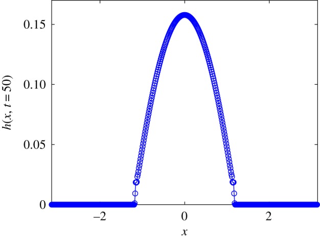
To understand the results in figure 6, a plot of $f_{\alpha }(\eta ,t):=t^{-1/7}\overline{h}(\eta t^{1/7},t)$, with ηt^1/7 = x is shown in figure 7, for t = 50. The numerical solution is compared with a solution of the ordinary differential equation f² f″′ = ηf/7, which is the (singular) similarity equation for the un-regularized dynamics (1.1). The ordinary differential equation is seeded with the initial condition f′(0) = 0; the additional required initial conditions on f(0) and f″(0) are fed in from the numerical solution of the partial differential equation; specifically, $f(0)=f_{\alpha }(0,t=50)$, and $f^{″}(0)=f_{\alpha }(0,t=50)$. It can be seen that the profiles of $f_{\alpha }(\eta ,t)$ and f(η) agree for |η| ≪ 1. Once the macroscopic contact line at η ≈ 1 is reached, the singular nature of the solution of the un-regularized problem becomes apparent, and f(η) diverges. One may take this as an equivalent definition of the macroscopic contact line, i.e. equivalent to the operational definition (3.9). By contrast, it is precisely in this region where the smooth nature of the solution of the regularized problem begins to appear, and $f_{\alpha }(\eta ,t)$ tends to zero as |η| → ∞.

Figure 7.

Comparison of the solution of the regularized problem (3.3) in similarity variables at t = 50 with the numerical solution of the unregularized problem f²f″′ = ηf/7. Unadorned solid line: regularized problem. Line with circles: unregularized problem. (Online version in colour.)

To understand the far-field structure of the diffuse free-surface height, we plot in figure 8 the numerical value of $\overline{h}(x,t=50)$, on a semilogarithmic scale. The tail of the profile shows a clear exponential decay $\overline{h}(x,t)\sim {\text{e}}^{-|x-x_{\text{m}}|/\alpha }$. Indeed, it is clear from figures 7 and 8 that the late-time solution of the regularized model (3.3) with the smoothing kernel (3.1) is a patchwork of two distinct types of space–time behaviour:

$$\overline{h}(x,t)\sim \{\begin{array}{ll}{t}^{-1/7}f(\frac{x}{t^{1/7}}),& x\ll x_{\text{m}}(t),\\ A(t){\text{e}}^{-|x-x_{\text{m}}(t)|/\alpha },& |x|\gg x_{\text{m}}(t),\end{array}$$ 3.10

in which the solution judiciously matches between the two extremes such that x_m(t) ∼ t^1/7, in agreement with Tanner’s Law.

Figure 8.

Plot of $\overline{h}(x,t=50)$ showing the spatial structure of the solution in the tail, for |x| ≫ x_m. (Online version in colour.)

(d). Discussion

In the light of the numerical results in figures 4–8, it is possible to ascribe a physical meaning to the filter width α. In the droplet core, the shape of the numerically simulated droplet is the same as that described by the standard thin-film equation (1.1), meaning the geometric diffuse-interface method properly describes the physics of droplet spreading in that region. In the droplet tail, the numerically simulated droplet inherits the exponential decay of the applied filter function. In fact, it is thought that real droplets exhibit a precursor film in this region, which extends beyond the droplet core, but which nevertheless decays algebraically to zero [13]. The precursor film has a characteristic thickness ℓ given by the surface tension and the parameters of a potential function (cf. equation (1.8); see also [6,13]). Therefore, in this small region, the geometric diffuse-interface method exhibits model uncertainty. Thus, the use of a filtered free-surface height is an expression of uncertainty in the model’s prediction for the free-surface height in the droplet tail—the lengthscale on which this uncertainty appears is α, and α may in turn be physically associated with ℓ in the theory in [13].

The numerical solutions use $\overline{h}$ as a dynamical variable. Therefore, the variable $h=(1-{\alpha }^2{\mathrm{\partial }}_x^2)\overline{h}$ plays a diagnostic role. A snapshot of h for the above numerical parameters is shown in figure 9. From the figure, it is apparent that h = 0 for |x| ≫ x_m(t), this is consistent with $\overline{h}(x,t)\sim A(t){\text{e}}^{-|x-x_{\text{m}}(t)|/\alpha }$ for |x| ≫ x_m(t), where A(t) is a time-dependent prefactor. We have deliberately retained the numerical gridpoints in figure 9. These gridpoints show an apparent jump discontinuity in h(x, t) near the position of the macroscopic contact line. In the sharp-interface description of contact-line motion, the moving contact line is associated with a logarithmic singularity in ∂_x h (cf. equation (1.7)). In the present geometric diffuse-interface method, however, the moving contact line expressed in the solution for $\overline{h}(x,t)$ is associated with a jump discontinuity manifested in h(x, t). This is demonstrated by the following theorem:

Figure 9.

Snapshot of the sharp free-surface height h(x, t) at t = 50. Numerical parameters as before. (Online version in colour.)

Theorem 3.2. —

Consider the solution h(x, t) to equation (2.5). Regarding the spatial variable x, if h(x, t) is in the function class C⁰( − ∞, ∞) and piecewise differentiable on ( − ∞, ∞), then there is no moving-contact-line solution to equation (2.5).

Proof. —

We suppose that there is a moving contact-line solution h(x, t) = ϕ(x, x₀) H(x − x₀)H(x + x₀) to equation (2.5), where x₀(t) is the microscopic contact line, i.e. the minimum positive value of x for which h(x₀, t) = 0. Here also, H(s) denotes the Heaviside function, and ϕ(x, x₀) is a differentiable function on the interval ( − x₀, x₀), which by the assumption of the moving-contact-line solution satisfies

$$\mathit{\Phi }(x_0):={\frac{\mathrm{\partial }\varphi }{\mathrm{\partial }{x}_0}|}_{x=x_0}\text{and}\mathit{\Phi }(x_0)\ne 0.$$

We apply this solution to equation (2.5) and integrate from x = −∞ to x = ∞, to obtain

$$\mathit{\Phi }(x_0)\left(\frac{\mathrm{d}{x}_0}{\mathrm{d}t}\right)={\int }_{-\mathrm{\infty }}^{\mathrm{\infty }}\frac{\mathrm{\partial }}{\mathrm{\partial }x}[h\mu (h,\overline{h})K\ast {\mathrm{\partial }}_{xx}(K\ast h)]\mathrm{d}x.$$

If h ∈ C⁰( − ∞, ∞) in the spatial variable and if h is piecewise differentiable also in the spatial variable, then the integral on the right-hand side can be broken up into different parts and evaluated to give zero, giving Φ(x₀)(dx₀/dt) = 0, hence dx₀/dt = 0, i.e. no moving contact line. ▪

Therefore, we conclude that the moving contact line in the numerical simulations corresponds to a sharp free-surface height h(x, t) which is piecewise differentiable, with jump discontinuities. As such, the sharp free-surface height h(x, t) satisfies equation (2.5) in a weak sense, with h ∈ C⁻¹( − ∞, ∞). (That is, h possesses a finite number of jump discontinuities). Using the convolution (3.1), we can conclude that $\overline{h}\in C^1(-\mathrm{\infty },\mathrm{\infty })$. We furthermore look at the convolution of equation (2.5), (i.e. equation (3.3)). This is the equation satisfied by $\overline{h}$. By counting derivatives on both sides of equation (3.3), one finds consistency with $\overline{h}\in C^1(-\mathrm{\infty },\mathrm{\infty })$. This result indicates that $\overline{h}$ satisfies equation (3.3) in a strong sense. We emphasize that although this discussion is consistent with the very precise numerical simulations carried out herein, a rigorous proof that $\overline{h}\in C^1(-\mathrm{\infty },\mathrm{\infty })$ has not yet been established. This question will be the subject of future work.

4. Conclusion

In summary, we have introduced a regularized thin-film equation which describes contact-line motion. The method does not rely on either a slip length or a precursor film. The method is inspired by the diffuse-interface concept, and it involves a smoothened or diffuse free-surface profile $\overline{h}(x,t)$. However, the method still contains a sharp interface, which can be obtained via deconvolution. The method reproduces Tanner’s Law for droplet spreading. Based on the numerical results and on counting the derivatives in the regularized thin-film equation, the diffuse profile $\overline{h}$ gives rise to a strong solution of the thin-film equation. These numerical results still need to be checked rigorously using theoretical methods (e.g. along the lines of [38]). The main advantages of the present model are its computational simplicity and robustness, as well as the future scope for using singular solutions as an additional simple but highly accurate computational solution method. Because of the model’s inherent computational simplicity, the model in its present guise can also be used as a description for spreading over heterogeneous surfaces, by introducing a spatial dependence into the lengthscale α, e.g. letting K*f = {1 − ∂_x(α²(x)∂_x]}⁻¹f in equation (3.1).

The model as formulated currently allows only for indefinite droplet spreading, corresponding to perfectly wetting fluids, and hence, a zero equilibrium macroscopic contact angle. To allow for non-zero equilibrium macroscopic contact angles, the model will require the introduction of additional physics, for instance, by adding a body-force potential of the Van der Waals type to equation (2.5). Equally, the model may be extended beyond the limit of lubrication theory, by combining the theoretical arguments in §2 with the general level-set formulation of two-phase flow. In this way, it is hoped that the present relatively simple model can serve as a template for geometric diffuse-interface methods for general two-phase flows.

Appendix A. Convergence analysis

In this appendix, we look at the convergence of the numerical method for the base case considered in §3 with α = 0.05, L = 2π, N = 500 and Δt = 10⁻². We show the effect of varying the number of grid points N and the timestep Δt. In this way, we demonstrate that the numerical results shown in §3 are converged. As such, the structure of $\overline{h}(x,t)$ is shown in figure 10a for Δt = 10⁻², t = 100 and various values of N. There is no visible change in the structure of $\overline{h}(x,t)$ when N is varied between 250 and 1000. Similarly, the position of the macroscopic contact line x_m(t) is plotted in figure 10b for the various values of N between 250 and 1000. There is little or no difference between the different plots of x_m(t) versus t for the various values of N. In figure 11, we further show the time evolution of x_m(t) for fixed N = 500 and various values of Δt. Again, there is little or no difference between the different plots of x_m(t) showing that the numerical results presented in the main paper are converged.

Figure 10.

Convergence study: effect of varying N at fixed Δt = 10⁻². The snapshots in (a) are taken at t = 100. (Online version in colour.)

Figure 11.

Convergence study: effect of varying Δt on the plot of the macroscopic contact line position x_m(t). (Online version in colour.)

Finally, it can be noted that the convergence of the numerical method is rather sensitive to the choice of mobility. For instance, using $\overline{\mu }=h^2$ rather than equation (2.12) leads to non-convergent results. The choice $\overline{\mu }=h^2$ corresponds to the Navier–Stokes equations in the lubrication limit with a regularized pressure p = −K*∂_xx(K*h) but the application of the no-stress boundary condition ∂u/∂y = 0 on y = h rather than on $y=\overline{h}$. The non-convergence of the numerical results in this instance underlines the importance of using the diffuse-interface $\overline{h}$ consistently in the formulation of the interfacial stress conditions.

Appendix B. Sensitivity analysis

In this appendix, we look at the sensitivity of the numerical results for the base case considered in §3 with α = 0.05, L = 2π, N = 500 and Δt = 10⁻². Specifically, we look at the sensitivity of the results with respect to variations in α and the kernel K. We keep N = 500 and Δt = 10⁻² fixed, as the results in appendix A have demonstrated that these values are sufficient for the numerical results to have converged. In figure 12a, we show the effect on the macroscopic contact line of varying α—these effects are small. In figure 12b, we show the effect on the macroscopic contact line of choosing a kernel $K={(1-{\alpha }^2{\mathrm{\partial }}_x^2+(1/2){\alpha }^4{\mathrm{\partial }}_x^4)}^{-1}$ instead of $K={(1-{\alpha }^2{\mathrm{\partial }}_x^2)}^{-1}$—the effect is negligible for regarding the motion of the macroscopic contact line.

Figure 12.

Sensitivity analysis. (a) Effect on results of varying α, with $K={(1-{\alpha }^2{\mathrm{\partial }}_x^2)}^{-1}$ (b) Effect on results of varying the kernel function, at fixed α = 0.05. In each case, L = 2π, N = 500 and Δt = 10⁻². (Online version in colour.)

Data accessibility

This article has no additional data.

Authors' contributions

All authors contributed equally to this research.

Competing interests

We declare we have no competing interests.

Funding

This work has been produced as part of ongoing work within the ThermaSMART network. The ThermaSMART network has received funding from the European Union’s Horizon 2020 research and innovation programme under the Marie Sklodowska–Curie grant agreement No. 778104. D.H. was partially supported by EPSRC Standard (grant no. EP/N023781/1]), entitled, ‘Variational principles for stochastic parametrizations in geophysical fluid dynamics’. C.T. acknowledges support from the Alexander von Humboldt Foundation (Humboldt Research Fellowship for Experienced Researchers) as well as from the German Federal Ministry for Education and Research