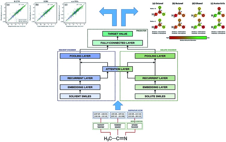
 We introduce Delfos, a novel, machine-learning-based QSPR method which predicts solvation free energies for generic organic solutions.
Abstract
Prediction of aqueous solubilities or hydration free energies is an extensively studied area in machine learning applications in chemistry since water is the sole solvent in the living system. However, for non-aqueous solutions, few machine learning studies have been undertaken so far despite the fact that the solvation mechanism plays an important role in various chemical reactions. Here, we introduce Delfos (deep learning model for solvation free energies in generic organic solvents), which is a novel, machine-learning-based QSPR method which predicts solvation free energies for various organic solute and solvent systems. A novelty of Delfos involves two separate solvent and solute encoder networks that can quantify structural features of given compounds via word embedding and recurrent layers, augmented with the attention mechanism which extracts important substructures from outputs of recurrent neural networks. As a result, the predictor network calculates the solvation free energy of a given solvent–solute pair using features from encoders. With the results obtained from extensive calculations using 2495 solute–solvent pairs, we demonstrate that Delfos not only has great potential in showing accuracy comparable to that of the state-of-the-art computational chemistry methods, but also offers information about which substructures play a dominant role in the solvation process.
1. Introduction
The most common strategies to predict biological or physicochemical properties of chemical compounds are ab initio quantum mechanical approaches1–9 like Hartree–Fock (HF) or density functional theory (DFT) and the molecular dynamics (MD) simulation method based on classical Newtonian and statistical mechanics.10–13 These methods with precisely defined theoretical backgrounds have been successfully used in calculating various features of chemical compounds. However, such methods have limitations in computational resources and time costs since they require an enormous amount of numerical calculations. As an alternative, recent successes in the machine learning (ML) technique and its implementation in cheminformatics are promoting broad applications of ML in chemical studies. Quantitative structure–activity relationship (QSAR) or quantitative structure–property relationship (QSPR) analysis is one of such techniques which predict various properties of a given compound from its empirical or structural features.14,15 The underlying architecture of QSAR/QSPR consists of two elementary mathematical functions.15 One is the encoding function, which encodes the chemical structure of the given compound into a molecular descriptor. The other, the mapping function, predicts the target property (or activity) that we intend to find out using the encoded descriptor.
There have been various molecular descriptors proposed to represent structural features of compounds efficiently. For example, we can feature a given molecule with simple enumerations of empirical properties like molecular weights, rotatable bonds, the number of hydrogen bond donors and acceptors, or some pre-experimental or pre-calculated properties.16 On the other hand, molecular fingerprints, which are another option, are commonly used in cheminformatics to estimate the chemical ‘difference’ between more than two compounds.17 They usually have a fixed size of a binary sequence and are easily obtainable from SMILES with pre-defined criteria. Graphical representation of molecules based on graph theory is another major encoding method in QSAR/QSPR which has received great attention in recent days.18,19 It has exhibited outstanding prediction performances in diverse chemical or biophysical properties.20
The mapping function extracts properties which we want to know about from encoded molecular features of the given compound via a classification or regression method. We can use any suitable machine learning method for mapping functions15,20 such as random forests (RF), support vector machines (SVM), neural networks (NNs), and so on. Among these diverse technical options, NN seems to be the method which has shown the most rapid advances in recent years,16,21–25 on the strength of the theoretical advances26 and evolution of computational power. Many studies have already been performed to show that various chemical or biophysical properties of compounds are obtainable from the QSAR/QSPR combined with machine learning techniques.16,20–25,27,28
Solvation is one of the most fundamental processes occurring in chemistry, and many theoretical and computational studies have been performed to calculate solubilities or solvation free energies using a variety of methodologies.29,30 For example, we can roughly guess solubilities using solvation parameters, but solvation parameters only provide the relative order, not the quantitative value.31 The general solubility equation (GSE) enables us to calculate solubilities from some empirical parameters, but it only provides solubilities for aqueous solutions.32Ab initio1–7 or MD simulations10–13 provide us with more concrete, accurate results and more in-depth knowledge about the solvation mechanism, but they have practical limitations due to high usage of computational resources as mentioned before.
Recent studies demonstrated that QSPR with ML successfully predicts aqueous solubilities or hydration free energies of diverse solutes.16,20,21,25,33,34 They also proved that ML guarantees faster calculations than computer simulations and more precise estimations than GSE estimation; a decent number of models showed accuracies comparable to ab initio solvation models.20 However, the majority of QSPR predictions for solubilities have been limited to cases of aqueous solutions. For non-aqueous solutions, few studies have been undertaken to predict the solubility despite the fact that predicting solubilities plays an important role in the development of varied fields of chemistry, e.g., organic synthesis,35 electrochemical reactions in batteries,36 and so on.
In the present work, we introduce Delfos (deep learning model for solvation free energies in generic organic solvents), which is a QSPR model combined with a recurrent neural network (RNN) model. Delfos is specialized in predicting solvation free energies of organic compounds in various solvents, and the model has three primary sub-neural networks: the solvent and solute encoder networks and the predictor network. For basic featurization of a given molecule, we use the word embedding technique.34,37 We calculate solvation energies of 2495 pairs of 418 solutes and 91 solvents38 and demonstrate that our model shows a performance as good as that of the best available quantum chemical methods2,6,8,11 when the neural network is trained with a sufficient chemical database.
The rest of the present paper is outlined as follows: Section 2 describes the embedding method for the molecular structure and overall architecture of the neural network. In Section 3, we mainly compare the performance of Delfos with both MD and ab initio simulation strategies3,6,8,11 and discuss database sensitivity using the cluster cross-validation method. We also visualize important substructures in solvation via the attention mechanism. In the last section, we conclude our work.
2. Methods
2.1. Word embedding
Natural language processing (NLP) is one of most cutting-edge subfields of computer science in varied applications of machine learning and neural networks.37,39–42 To process human languages using computers, we need to encode words and sentences and extract their linguistic properties. The process is commonly implemented via the word embedding method.37,39 To perform this task, unsupervised learning schemes such as skip-gram and continuous bag of words (CBOW) algorithms generate a vector representation of the given word in an arbitrary vector space.37,39 If the corresponding vector space is well-defined, one can deduce the semantic or syntactic features of the given word from the position of the embedded vector, and the inner product of two vectors that correspond to two different words provides information about their linguistic relations.
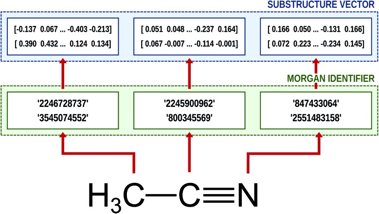
It is worthwhile to note that we can employ the embedding technique for chemical or biophysical processes if we consider an atom or a substructure to be a word and a compound to be a sentence.33,34,43 In this case, positions of molecular substructures in the embedded vector space represent their chemical and physical properties, instead of linguistic information. There are already bio-vector models43 that have been developed which encode sequences of proteins or DNAs, and atomic-vector embedding models have been introduced recently to encode structural features of chemical compounds.33,34 Mol2Vec is one of such embedding techniques, and it generates vector representations of a given molecule from the molecular sentence.34 To make molecular sentences, Mol2Vec uses the Morgan algorithm44 that classifies identical atoms in the molecule. The algorithm is commonly used to generate ECFPs,45 which are the de facto standard in cheminformatics,17 and it creates identifiers of the given atom from the chemical environment in which the atom is positioned. An atom may have multiple identifiers depending on the pre-set maximum value of the radius rmax, which denotes the maximum topological distance between the given atom and its neighboring atoms. The atom itself is identified by r = 0, and additional substructure identifiers for adjacent atoms are denoted by r = 1 (nearest neighbor), r = 2 (next nearest neighbor), and so on. Since Mol2Vec has demonstrated promising performances in several applications of QSAR/QSPR,34 Delfos uses Mol2Vec as the primary encoding means. The schematic illustration of the embedding procedure for acetonitrile is shown in Fig. 1.
Fig. 1. Schematic illustration of the molecular embedding process for acetonitrile (SMILES: CC#N) and rmax = 1. The Morgan algorithm discriminates identifiers between two substructures: one is for itself (r = 0) and the other considers its nearest neighbor atoms (r = 1). Then the embedding layer calculates the vector representation from the given identifier.
2.2. Encoder-predictor network
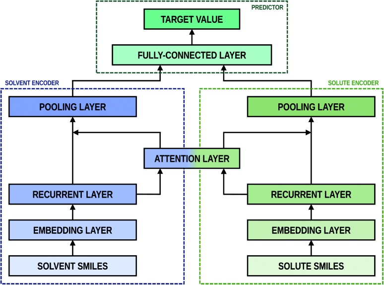
As shown in Fig. 2, the fundamental architecture of Delfos involves three sub-neural networks: the solvent and the solute encoders extract dominant structural features of the given compound from SMILES strings, while the predictor calculates the solvation energy of the given solvent–solute pair from their encoded features.
Fig. 2. The fundamental architecture of Delfos. Each encoder network has one embedding and one recurrent layer, while the predictor has a fully connected MLP layer. Two encoders share an attention layer, which weights outputs from recurrent layers. Black arrows indicate the flow of input data.
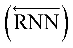
The primary architecture of the encoder is based on two bidirectional recurrent neural networks (BiRNNs).46 The network is designed for handling sequential data and we consider the molecular sentence [x1, …, xN] to be a sequence of embedded substructures, xi. RNNs may have a failure when input sequences are lengthy; gradients of the loss function can be diluted or amplified because of accumulated precision error from the backpropagation process.47 The excessive or restrained gradient may cause a decline in learning performance, and we call these two problems vanishing or exploding gradients. To overcome these limits which stem from lengthy input sequences, (copy) one may consider using both the forward-directional RNN 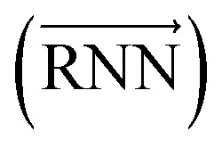 and backward-directional RNN
  within a single layer:
 |
1a |
 |
1b |
 |
1c |
In eqn (1), xi is the embedded atomic vector of a given molecule, 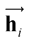 and
and 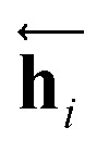 are the hidden state outputs of each recurrent unit, and
 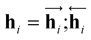 represents the concatenation of two hidden states, respectively. More advanced versions of RNN, like the long short-term memory48 (LSTM) or gated recurrent unit49 (GRU) networks, are widely used to handle lengthy input sequences. They introduce gates in each RNN cell state to memorize important information of the previous cell state and minimize vanishing and exploding gradient problems.
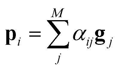
After the RNN layers, the molecular sentences of both the solvent X = [x1, …, xN] and the solute Y = [y1, …, yM] are converted to hidden states, H = [h1, …, hN] and G = [g1, …, gM], respectively. Each hidden state is then inputted into the shared attention layer and weighted. The attention mechanism, which was originally proposed to enhance performances of a machine translator,40 is an essential technique in diverse NLP applications nowadays.41,42 Principles of the attention start from the definition of the score function of hidden states and its normalization with the softmax function:
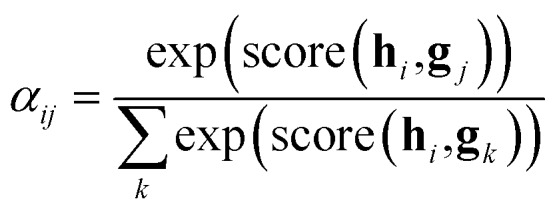 |
2a |
 |
2b |
| score(hi,gj) = hi·gj | 2c |
There are various score functions that have been introduced to achieve efficient predictions,40–42 and among them we use Luong's dot-product attention42 in eqn (2c) as a score function since it is computationally efficient. The solvent context, P = αG denotes an emphasized hidden state H with the attention alignment, α. We also obtain the solute context Q using the same procedure. The context weighted from the attention layer is an L × 2D matrix, where L is the sequence length and D is the dimensions of two RNN hidden layers since we use a bidirectional RNN (BiRNN). Two max-pooling layers, which are the last part of each encoder, reduce contexts H, G, P, and Q to 2D-dimensional feature vectors u and v:42
| u = MaxPooling([h1;p1,…,hN;pN]) | 3a |
| v = MaxPooling([g1;q1,…,gM;qM]) | 3b |
The predictor has a single fully connected perceptron layer with a rectifier unit (ReLU) and an output layer. It uses the concatenated feature of the solvent and solute [u;v] as an input. The overall architecture of our model is shown in Fig. 2. We also consider encoders without RNNs and attention layers in order to quantify the impact of these layers on prediction performances of the network; each encoding network contains only the embedding layer and is directly connected to the MLP layer. The solvent and solute features are simple summations of atomic vectors, 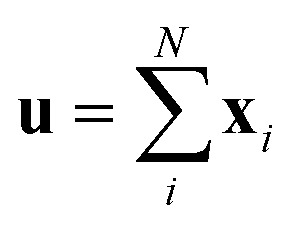 and
and  , respectively. This model was initially used for gradient boosting (GBM) regression analysis for aqueous solubilities and toxicities.34
3. Results and discussion
3.1. Computational setup and results
We use the Minnesota solvation database38 (MNSOL) as the dataset over which we train and test, and it provides 3037 experimental measures of free energies of solvation and transfer energies for 790 unique solutes in 92 solvents. Because the MNSOL only contains common names of compounds, we perform an automated search process using the PubChemPy50 script and obtain SMILES strings of compounds from the PubChem database. There are 363 results for charged solutes and 144 results for transfer free energies in the MNSOL which are excluded from the machine learning dataset, and 35 results of solvent–solute combinations are not valid in PubChem. We finally prepare SMILES specifications of 2495 solutions for 418 solutes and 91 solvents for the machine learning input.
For implementation of the neural networks, we use the Keras 2.2.4 framework51 with TensorFlow 1.12 backend.52 At the very first stage, the Morgan algorithm for r = 0 and r = 1 generates molecular sentences of the solvent and solute from their SMILES strings. Then the given molecular sentence is embedded into a sequence of 300-dimensional substructure vectors using the pre-trained Word2Vec model available at ; https://github.com/samoturk/mol2vec, which contains information on ∼20 000 000 compounds and ∼20 000 substructures from ZINC and ChEMBL databases.34 We consider BiLSTM and BiGRU layers in both solvent and solute encoders to compare their performances. Since our model is a regression problem, we use mean squared error (MSE) as the loss function.
We employ 10-fold cross-validation (CV) for secure representation of the test data because the dataset we use has a limited number of experimental measures; the total dataset is uniformly and randomly split into 10 subsets, and we iteratively choose one of the subsets as a test set and the training run uses the remaining 9 subsets. Consequentially, a 10-fold CV task performs 10 independent training and test runs, and relative sizes of the training and test sets are 9 to 1. We use Scikit-Learn library53 to implement the CV task and perform an extensive grid search for tuning hyperparameters: learning algorithms, learning rates, and dimensions of hidden layers. We select the stochastic gradient descent (SGD) algorithm with Nesterov momentum, whose learning rate is 0.0002 and momentum is 0.9. Optimized hidden dimensions are 150 for recurrent layers and 2000 for the fully connected layer. To minimize the variance of the test run, we take averages for all results over 9 independent random CVs, split from different random states.
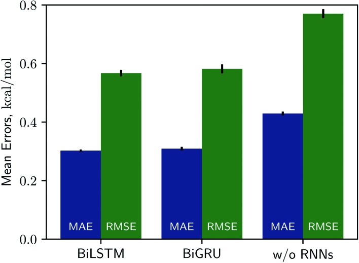
Solvation free energies calculated from the MNSOL using attentive BiRNN encoders are exhibited in Fig. 3 and 4. Prediction errors for the BiLSTM model are ±0.57 kcal mol–1 in RMSE and ±0.30 kcal mol–1 in MAE, and the Pearson correlation coefficient R2 = 0.96, while results from the BiGRU model indicate that there is no meaningful difference between the two recurrent models. The encoder without BiRNN and attention layers produces much more inaccurate results, whose error metrics are ±0.77 kcal mol–1 in RMSE and ±0.43 kcal mol–1 in MAE, and the R2 value is 0.92, respectively.
Fig. 3. Benchmark chart for three kinds of encoder networks, for two metrics (MAE and RMSE). The BiLSTM and the BiGRU models show no significant differences, while they make relatively inaccurate predictions without recurrent networks. All results are averaged over 9 independent test runs and black lines on top of boxes denote variances.
Fig. 4. Scatter plot for true (x-axis) and ML predicted (y-axis) values of solvation energies in three different models: (a) BiLSTM, (b) BiGRU, and (c) without recurrent layers. All results are averaged over 9 independent 10-fold CV runs.
We cannot directly compare our results with those of other ML models because Delfos is the first ML-based study using the MNSOL database. Nonetheless, several studies on aqueous systems have previously calculated solubilities or hydration free energies using various ML techniques and molecular descriptors.16,20,21,25,33,34 For comparison, we have tested our neural network model for the hydration free energy. A benchmark study from Wu et al.20 provides hydration energies of 642 small molecules in a group of QSPR/ML models. Their RMSEs were up to 1.15 kcal mol–1 while our prediction from the BiLSTM encoder attains 1.19 kcal mol–1 for the same dataset and split method (see the ESI†). This result suggests that our neural network model guarantees considerably good performances even in a specific solvent of water.
Meanwhile, for studies which are not ML-based, there are several results from both classical and quantum-mechanical simulation studies that use the MNSOL as the reference database.3–6,8,11,13 In Table 1, we choose two DFT studies which employ several widely used QM solvation models3,8 for comparison with our proposed ML model: solvation model 8/12 (SM8/SM12), the solvation model based on density (SMD), and the full/direct conductor-like screening model for realistic solvation (COSMO-RS/D-COSMO-RS). While all of these QM methods exhibited excellent performances when considering a chemical accuracy of 1.0 kcal mol–1, full COSMO-RS is a noteworthy solvation model since it is believed to be a state-of-the-art method which shows the best accuracy.9 This is realized by statistical thermodynamics treatment on the polarization charge densities, which helps COSMO-RS with making successful predictions even in polar solvents where the key idea of the dielectric continuum solvation collapses.1,7,9 Resultingly, COSMO-RS calculations with the BP86 functional and TZVP basis set achieved 0.52 kcal mol–1 for 274 aqueous solvents, 0.41 kcal mol–1 for 2072 organic solvents, and 0.43 kcal mol–1 for the full dataset in mean absolute error.8
Table 1. Comparison between encoder-predictor networks and various quantum-mechanical solvation models for aqueous and non-aqueous solutions. The error metric is MAE and kcal mol–1. Data in bold are our results, while QM results are taken from the work of Marenich et al.3 and Klamt and Diedenhofen8.
| Solvent | Method | N data | MAE | Ref. |
| Aqueous | SM12CM5/B3LYP/MG3S | 374 | 0.77 | Marenich et al.3 |
| SM8/M06-2X/6-31G(d) | 366 | 0.89 | Marenich et al.3 | |
| SMD/M05-2X/6-31G(d) | 366 | 0.88 | Marenich et al.3 | |
| COSMO-RS/BP86/TZVP | 274 | 0.52 | Klamt and Diedenhofen8 | |
| D-COSMO-RS/BP86/TZVP | 274 | 0.94 | Klamt and Diedenhofen8 | |
| Delfos/BiLSTM | 374 | 0.64 | ||
| Delfos/BiGRU | 374 | 0.68 | ||
| Delfos w/o RNNs | 374 | 0.90 | ||
| Non-aqueous | SM12CM5/B3LYP/MG3S | 2129 | 0.54 | Marenich et al.3 |
| SM8/M06-2X/6-31G(d) | 2129 | 0.61 | Marenich et al.3 | |
| SMD/M05-2X/6-31G(d) | 2129 | 0.67 | Marenich et al.3 | |
| COSMO-RS/BP86/TZVP | 2072 | 0.41 | Klamt and Diedenhofen8 | |
| D-COSMO-RS/BP86/TZVP | 2072 | 0.62 | Klamt and Diedenhofen8 | |
| Delfos/BiLSTM | 2121 | 0.24 | ||
| Delfos/BiGRU | 2121 | 0.24 | ||
| Delfos w/o RNNs | 2121 | 0.36 |
For the proposed ML models, Delfos with BiLSTM shows a comparable accuracy in the water solvent, for which MAE is 0.64 kcal mol–1. Delfos makes much better predictions in non-aqueous organic solvents; machine learning for 2121 non-aqueous systems results in 0.24 kcal mol–1, which is 44% that of SM12CM5 and 59% that of COSMO-RS. However, one may argue that K-fold CV from random split does not produce the real prediction accuracy of the model. That is, the random-CV results only indicate the accuracy for trained or practiced chemical structures. Accordingly, one may ask the following questions. For example, will the ML model ensure comparable prediction accuracy in “structurally” new compounds? What happens if the ML model cannot learn sufficiently varied chemical structures? We will discuss these questions in the next section.
3.2. Transferability of the model for new compounds
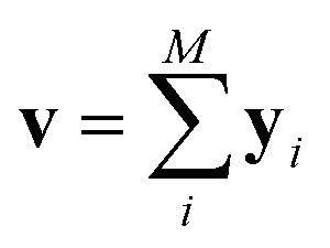
Since our study uses techniques of machine learning with empirical data from experimental measures, there is a likelihood that Delfos would not guarantee prediction accuracy for structurally new solvents or solutes which are not present in the dataset, although the MNSOL contains a considerable number of commonly used solvents and solutes.38 In order to investigate this potential issue, we perform another training and test run with cluster cross-validation,54,55 instead of using the random-split CV. As a start, we individually obtain 10 clusters for solvents and solutes using the K-mean clustering algorithm and the molecular vector. The molecular vector is a simple summation of substructure vectors used for the simple MLP model without RNN encoders:34 for solvents and
  for solutes, respectively. Then, we iteratively perform the cross-validation process over each cluster. The size of each cluster is [422, 482, 186, 231, 443, 243, 143, 251, 15, 79] for solvents and [401, 672, 514, 75, 64, 6, 512, 54, 42, 155] for solutes, respectively.
Results from the solvent and the solute cluster CV tasks shown in Table 2 exhibit generalized expectation error ranges for new solvents or solutes which are not in the dataset. Winter et al.55 reported that the split method based on the clustering exhibits an apparent degradation of prediction performances in various properties; we find that our proposed model exhibits a similar tendency as well. For the BiLSTM encoder model, increments of MAE are 0.52 kcal mol–1 for the solvent clustering and 0.69 kcal mol–1 for the solute clustering. The reason why the random K-fold CV exhibits superior performances is obvious; if we have a pair 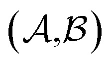 of solvents
  and solutes
  in the test set and the training set has
 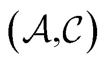 and
and  pairs, then both
  and
and 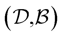 could enhance the prediction accuracy of
  . However, the clustering limits the location of a specific compound, and pairs of specific solvents or solutes should be either in the test set or the training set.
Table 2. Prediction accuracy of the random-split CV, the solvent and solute cluster CV using the K-mean algorithm, and several theoretical solvation models for four different organic solvents: toluene (C6H5CH3), chloroform (CHCl3), acetonitrile (CH3CN), and dimethyl sulfoxide ((CH3)2SO), respectively. Units of MAE and RMSE are kcal mol–1.
| Solvent | Method | N data | MAE | RMSE | Ref. |
| All | COSMO/BP86/TZVP | 2346 | 2.15 | 2.57 | Klamt and Diedenhofen8 |
| COSMO-RS/BP86/TZVP | 2346 | 0.42 | 0.75 | Klamt and Diedenhofen8 | |
| SMD/PM3 | 2500 | — | 4.8 | Kromann et al.6 | |
| SMD/PM6 | 2500 | — | 3.6 | Kromann et al.6 | |
| Delfos/random CV | 2495 | 0.30 | 0.57 | ||
| Delfos/solvent clustering | 2495 | 0.82 | 1.45 | ||
| Delfos/solute clustering | 2495 | 0.99 | 1.61 | ||
| Toluene | MD/GAFF | 21 | 0.48 | 0.63 | Mohamed et al.11 |
| MD/AMOEBA | 21 | 0.92 | 1.18 | Mohamed et al.11 | |
| COSMO/BP86/TZVP | 21 | 2.17 | 2.71 | Klamt and Diedenhofen8 | |
| COSMO-RS/BP86/TZVP | 21 | 0.27 | 0.34 | Klamt and Diedenhofen8 | |
| Delfos/random CV | 21 | 0.16 | 0.37 | ||
| Delfos/solvent clustering | 21 | 0.66 | 1.10 | ||
| Delfos/solute clustering | 21 | 0.93 | 1.46 | ||
| Chloroform | MD/GAFF | 21 | 0.92 | 1.11 | Mohamed et al.11 |
| MD/AMOEBA | 21 | 1.68 | 1.97 | Mohamed et al.11 | |
| COSMO/BP86/TZVP | 21 | 1.76 | 2.12 | Klamt and Diedenhofen8 | |
| COSMO-RS/BP86/TZVP | 21 | 0.50 | 0.66 | Klamt and Diedenhofen8 | |
| Delfos/random CV | 21 | 0.35 | 0.56 | ||
| Delfos/solvent clustering | 21 | 0.78 | 0.87 | ||
| Delfos/solute clustering | 21 | 1.14 | 1.62 | ||
| Acetonitrile | MD/GAFF | 6 | 0.43 | 0.52 | Mohamed et al.11 |
| MD/AMOEBA | 6 | 0.73 | 0.77 | Mohamed et al.11 | |
| COSMO/BP86/TZVP | 6 | 1.42 | 1.58 | Klamt and Diedenhofen8 | |
| COSMO-RS/BP86/TZVP | 6 | 0.33 | 0.38 | Klamt and Diedenhofen8 | |
| Delfos/random CV | 6 | 0.29 | 0.39 | ||
| Delfos/solvent clustering | 6 | 0.74 | 0.82 | ||
| Delfos/solute clustering | 6 | 0.80 | 0.94 | ||
| DMSO | MD/GAFF | 6 | 0.61 | 0.75 | Mohamed et al.11 |
| MD/AMOEBA | 6 | 1.12 | 1.21 | Mohamed et al.11 | |
| COSMO/BP86/TZVP | 6 | 1.31 | 1.42 | Klamt and Diedenhofen8 | |
| COSMO-RS/BP86/TZVP | 6 | 0.56 | 0.73 | Klamt and Diedenhofen8 | |
| Delfos/random CV | 6 | 0.41 | 0.44 | ||
| Delfos/solvent clustering | 6 | 0.93 | 1.19 | ||
| Delfos/solute clustering | 6 | 0.91 | 1.11 |
For an additional comparison, Table 2 also contains results taken from SMD with semi-empirical methods,6 pure COSMO, COSMO-RS,8 and classical molecular dynamics11 for four organic solvents: toluene (C6H5CH3), chloroform (CHCl3), acetonitrile (CH3CN), and dimethyl sulfoxide ((CH3)2SO), respectively. Although the MD is based on classical dynamics, the results of the generalized amber force field (GAFF) tell us that an explicit solvation model with a suitable force field could make considerably good predictions. The bottom line of cluster CV is if the dataset for training contains at least one side of the solvent–solvent pair we want to estimate its solvation free energy, the expectation error of Delfos lies within a chemical accuracy of 1.0 kcal mol–1, which is the general error of the computer simulation scheme. Also, results for four organic solvents demonstrate that predictions from the cluster CV have an accuracy that is comparable with that of MD simulations using an AMOEBA polarizable force field.11
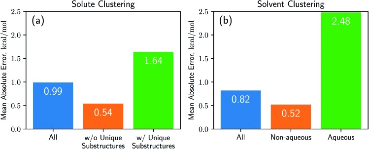
Results from the cluster CV highlight the necessity for discussion on the importance of database preparation. As described earlier, the cluster CV causes a considerable increase in prediction error, and we suspect that the degradation mainly comes from the decline in the diversity of the training set. Namely, the number of substructures that the neural network learns in the training process is not as many as the random CV if we use the cluster CV. To prove this speculation, we define unique substructures, which are substructures that only exists in the test cluster. As shown in Fig. 5, in the solute cluster CV, the MAE for 1226 pairs which don't have any unique substructures in solutes is 0.54 kcal mol–1, while the prediction error for the remaining 1269 solutions is 1.64 kcal mol–1. The solvent cluster CV shows more extreme results: the MAE for 374 aqueous solvents is 2.48 kcal mol–1, while non-aqueous solvents exhibit 0.52 kcal mol–1 in contrast. We believe that the outlying behavior of water is due to its distinctive nature. Water has only one unique substructure since the oxygen atom does not have any neighbors. So the solvent clustering makes the network unable to learn the structure of water in indirect ways, resulting in prediction failure. This logic tells us that the most critical thing is securing of the training dataset which contains as many kinds of solvents and solutes as possible. We believe that computational approaches would be as helpful as experimental measures for enriching structural diversity of the training data, given recent advances on QM solvation models2,3,8 such as COSMO-RS. Furthermore, since there are 418 solutes and 91 solvents in the dataset used,38 which make up 38 038 possible pairs, we expect Delfos and MNSOL to guarantee similar precision levels with the random CV for numerous systems.
Fig. 5. Results of cross-validation tasks using the K-mean clustering algorithm for (a) solutes and (b) solvents. We conclude that unique substructures in the given compounds are the main cause for the decline in prediction accuracy. Each encoder network includes a BiLSTM layer and we use the same hyperparameters which are optimized in the random CV task.
3.3. Visualization of the attention mechanism
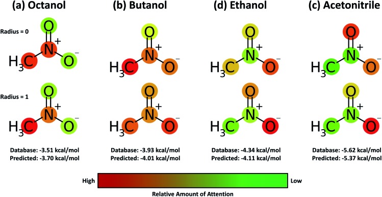
A useful aspect of the attention mechanism is that the model provides not only the prediction value of solvation energy of a given input but also a clue to why the neural network makes such a prediction based on the correlations between recurrent hidden states.25,33,41 In this section, we visualize how the attention layer operates, and verify how such correlations correspond well to chemical intuitions for inter-molecular interactions. The matrix of attention alignments, α, from eqn (2a) indicates which substructures in the given solvent and solute are strongly correlated with each other so that they play dominant roles in determining their solvation energy. In Fig. 6, we demonstrate attention alignments of a nitromethane (CH3NO2) solute in four different solvents: 1-octanol (C8H17OH, 3.51 kcal mol–1), 1-butanol (C4H9OH, 3.93 kcal mol–1), ethanol (C2H5OH, 4.34 kcal mol–1), and acetonitrile (CH3CN, 5.62 kcal mol–1). The scheme for visualizing attention alignments is as follows: (i) first, we calculate the average alignment ). The scheme for visualizing attention alignments is as follows: (i) first, we calculate the average alignment 〈α〉j of each substructure j of the solute over the entire solvent structure {i}, 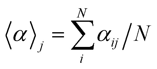 . (ii) Then, we get relative amounts of averaged alignments [α̃1, …, α̃M] by dividing by the maximum value, α̃j = = 〈α〉j/max(/max(〈α〉1, …, , …, 〈α〉M). (iii) Also, since the embedding algorithm used generates two substructure vectors per atom, we individually visualize two alignment maps, [α̃1, α̃3, …, α̃M–1] (for r = 0) and [α̃2, α̃4, …, α̃M] (for r = 1) for more simple and intuitive illustration. (iv) Finally, the color representation of each atom in Fig. 6 denotes the amount of α̃j; the neural network judges that red-colored substructures (higher α̃j) in the solute are more “similar” to the solvent and the model puts more weight on them during the prediction task. In contrast, green-colored substructures have a lower α̃j, which means they do not share similarities with the solvent molecule as much as the red-colored ones.
Fig. 6. Relative and mean attention alignment map for nitromethane in four different solvents: (a) octanol, (b) butanol, (c) ethanol, and (d) acetonitrile, respectively. Color representations denote that the neural network invests more weight on red, while green substructures have relatively low contributions towards the solvation energy.
Overall the results in Fig. 6 imply that the chemical similarity taken from the attention layer has a significant connection to a fundamental knowledge of chemistry like polarity or hydrophilicity. Each alcoholic solvent has one hydrophilic –OH group, and this results in increasing contributions of the nitro group in the solute as hydrocarbon chains of alcohols shorten. For the acetonitrile–nitromethane solution, the attention mechanism reflects the highest contributions of –NO2 groups due to the strong polarity and aprotic nature of the solvent. Although the attention mechanism seems to reproduce molecular interactions in a faithful way, we find that there is a defective prediction which does not agree with chemical knowledge. Two oxygen atoms O and –O– in the nitro group are indistinguishable due to the resonance structure; thus they must have equivalent contributions in any solvent, but we find that they show different attention scores in our model. We believe that these problems occur because the SMILES string of nitromethane (C[N+]( O)[O–]) does not encode the resonance effect in the nitro group. Indeed, the Morgan algorithm generates different identifiers for two oxygen atoms in the nitro group, [864 942 730, 2 378 779 377] for O and [864 942 795, 2 378 775 366] for –O–. The absence of resonance might be a problem worth considering when one intends to use word embedding models with SMILES strings,33,34,55 although estimated solvation energies for nitromethane from the BiLSTM model are within a moderate error range as shown in Fig. 6.
4. Conclusions
In the present study, we introduced a QSPR regression neural network for solvation energy estimation that is inspired by NLP. The proposed model has two separate encoder neural networks for solvents and solutes and a predictor neural network. Each encoder neural network is designed to encode the chemical structure of an input compound into the feature vector of a specific size. The encoding procedure is accomplished using the Mol2Vec embedding model34 and recurrent neural networks with the attention mechanism.40–42 The predictor neural network with fully connected MLP calculates the solvation free energy of a given solvent–solute pair using the feature vectors from encoders.
We performed extensive calculations on 2495 experimental values of solvation energies taken from the MNSOL database.38 From the random-CV task, we obtained mean averaged errors in solvation free energy of Delfos using BiLSTM as 0.64 kcal mol–1 for aqueous systems and 0.24 kcal mol–1 for non-aqueous systems. Our results demonstrate that the proposed model exhibits excellent prediction accuracy which is comparable with that of several well-known QM solvation models3,8 when the neural network is trained with sufficiently varied chemical structures, while the MLP model which does not contain recurrent or attention layers showed relatively deficient performances. A decline in performances of about 0.5 to 0.7 kcal mol–1 at the cluster CV tasks represents the accuracy for a structurally new compound, suggesting the importance of preparation of ML databases even though Delfos still demonstrates comparable predictions with some theoretical approaches such as MD using the AMOEBA force field11 or DFT with pure COSMO.8 The score matrix taken from the attention mechanism gives us an interaction map between the atoms and substructure; our model not only provides a simple estimation of target property but also offers important pieces of information about which substructures play a dominant role in solvation processes.
One of the most useful advantages of ML is flexibility; a single model can be used to learn and predict various databases.20 Also, our model may be applied to predict various chemical, physical, or biological properties especially focused on interactions between more than two different chemical species. One of the possible applications that we can consider is the prediction of chemical affinity and the possibility of various chemical reactions.56 Room-temperature ionic liquids might be another potential research topic became the interplay between cations and anions dominates their various properties, e.g., toxicity57 or electrochemical properties in supercapacitors.58,59 Thus, we expect that Delfos will be helpful in many further studies, and not only localized to the prediction of solvation energies.
Conflicts of interest
There are no conflicts to declare.
Supplementary Material
Acknowledgments
This research was supported by the Creative Materials Discovery Program through the National Research Foundation of Korea (NRF) funded by the Ministry of Science, ICT and Future Planning (NRF-2017M3D1A1039553).
Footnotes
†Electronic supplementary information (ESI) available. See DOI: 10.1039/c9sc02452b
References
- Klamt A. J. Phys. Chem. 1995;99:2224–2235. [Google Scholar]
- Cramer C. J., Truhlar D. G., Marenich A. V., Kelly C. P., Olson R. M. J. Chem. Theory Comput. 2007;3:2011–2033. doi: 10.1021/ct7001418. [DOI] [PubMed] [Google Scholar]
- Marenich A. V., Cramer C. J., Truhlar D. G. J. Chem. Theory Comput. 2013;9:609–620. doi: 10.1021/ct300900e. [DOI] [PubMed] [Google Scholar]
- Dupont C., Andreussi O., Marzari N. J. Chem. Phys. 2013;139:214110. doi: 10.1063/1.4832475. [DOI] [PubMed] [Google Scholar]
- Sundararaman R., Goddard W. A. J. Chem. Phys. 2015;142:064107. doi: 10.1063/1.4907731. [DOI] [PubMed] [Google Scholar]
- Kromann J. C., Steinmann C., Jensen J. H. J. Chem. Phys. 2018;149:104102. doi: 10.1063/1.5047273. [DOI] [PubMed] [Google Scholar]
- Klamt A., Eckert F., Arlt W. Annu. Rev. Chem. Biomol. Eng. 2010;1:101–122. doi: 10.1146/annurev-chembioeng-073009-100903. [DOI] [PubMed] [Google Scholar]
- Klamt A., Diedenhofen M. J. Phys. Chem. A. 2015;119:5439–5445. doi: 10.1021/jp511158y. [DOI] [PubMed] [Google Scholar]
- Klamt A. Wiley Interdiscip. Rev.: Comput. Mol. Sci. 2018;8:e1338. [Google Scholar]
- Shivakumar D., Williams J., Wu Y., Damm W., Shelley J., Sherman W. J. Chem. Theory Comput. 2010;6:1509–1519. doi: 10.1021/ct900587b. [DOI] [PubMed] [Google Scholar]
- Mohamed N. A., Bradshaw R. T., Essex J. W. J. Comput. Chem. 2016;37:2749–2758. doi: 10.1002/jcc.24500. [DOI] [PMC free article] [PubMed] [Google Scholar]
- Misin M., Fedorov M. V., Palmer D. S. J. Phys. Chem. B. 2016;120:975–983. doi: 10.1021/acs.jpcb.5b10809. [DOI] [PubMed] [Google Scholar]
- Genheden S. J. Comput.-Aided Mol. Des. 2017;31:867–876. doi: 10.1007/s10822-017-0059-9. [DOI] [PMC free article] [PubMed] [Google Scholar]
- Cherkasov A., Muratov E. N., Fourches D., Varnek A., Baskin I. I., Cronin M., Dearden J., Gramatica P., Martin Y. C., Todeschini R., Consonni V., Kuz’min V. E., Cramer R., Benigni R., Yang C., Rathman J., Terfloth L., Gasteiger J., Richard A., Tropsha A. J. Med. Chem. 2014;57:4977–5010. doi: 10.1021/jm4004285. [DOI] [PMC free article] [PubMed] [Google Scholar]
- Mitchell J. B. O. Wiley Interdiscip. Rev.: Comput. Mol. Sci. 2014;4:468–481. doi: 10.1002/wcms.1183. [DOI] [PMC free article] [PubMed] [Google Scholar]
- Delaney J. S. J. Chem. Inf. Comput. Sci. 2004;44:1000–1005. doi: 10.1021/ci034243x. [DOI] [PubMed] [Google Scholar]
- Cereto-Massagué A., Ojeda M. J., Valls C., Mulero M., Garcia-Vallvé S., Pujadas G. Methods. 2015;71:58–63. doi: 10.1016/j.ymeth.2014.08.005. [DOI] [PubMed] [Google Scholar]
- Kearnes S., Riley P. J. Comput.-Aided Mol. Des. 2016;30:595–608. doi: 10.1007/s10822-016-9938-8. [DOI] [PMC free article] [PubMed] [Google Scholar]
- Coley C. W., Barzilay R., Green W. H., Jaakkola T. S., Jensen K. F. J. Chem. Inf. Model. 2017;57:1757–1772. doi: 10.1021/acs.jcim.6b00601. [DOI] [PubMed] [Google Scholar]
- Wu Z., Ramsundar B., Feinberg E. N., Gomes J., Geniesse C., Pappu A. S., Leswing K., Pande V. Chem. Sci. 2018;9:513–530. doi: 10.1039/c7sc02664a. [DOI] [PMC free article] [PubMed] [Google Scholar]
- Lusci A., Pollastri G., Baldi P. J. Chem. Inf. Model. 2013;53:1563–1575. doi: 10.1021/ci400187y. [DOI] [PMC free article] [PubMed] [Google Scholar]
- Schütt K. T., Arbabzadah F., Chmiela S., Müller K. R., Tkatchenko A. Nat. Commun. 2017;8:13890. doi: 10.1038/ncomms13890. [DOI] [PMC free article] [PubMed] [Google Scholar]
- Gómez-Bombarelli R., Wei J. N., Duvenaud D., Hernández-Lobato J. M., Sánchez-Lengeling B., Sheberla D., Aguilera-Iparraguirre J., Hirzel T. D., Adams R. P., Aspuru-Guzik A. ACS Cent. Sci. 2018;4:268–276. doi: 10.1021/acscentsci.7b00572. [DOI] [PMC free article] [PubMed] [Google Scholar]
- Chen H., Engkvist O., Wang Y., Olivecrona M., Blaschke T. Drug Discovery Today. 2018;23:1241–1250. doi: 10.1016/j.drudis.2018.01.039. [DOI] [PubMed] [Google Scholar]
- Zheng S., Yan X., Yang Y., Xu J. J. Chem. Inf. Model. 2019;59:914–923. doi: 10.1021/acs.jcim.8b00803. [DOI] [PubMed] [Google Scholar]
- Schmidhuber J. Neural Networks. 2015;61:85–117. doi: 10.1016/j.neunet.2014.09.003. [DOI] [PubMed] [Google Scholar]
- Okamoto Y., Kubo Y. ACS Omega. 2018;3:7868–7874. doi: 10.1021/acsomega.8b00576. [DOI] [PMC free article] [PubMed] [Google Scholar]
- Faber F., Lindmaa A., von Lilienfeld O. A., Armiento R. Int. J. Quantum Chem. 2015;115:1094–1101. [Google Scholar]
- Sato H. Phys. Chem. Chem. Phys. 2013;15:7450. doi: 10.1039/c3cp50247c. [DOI] [PubMed] [Google Scholar]
- Skyner R. E., McDonagh J. L., Groom C. R., van Mourik T., Mitchell J. B. O. Phys. Chem. Chem. Phys. 2015;17:6174–6191. doi: 10.1039/c5cp00288e. [DOI] [PubMed] [Google Scholar]
- Barton A. F. M. Chem. Rev. 1975;75:731–753. [Google Scholar]
- Ran Y., Yalkowsky S. H. J. Chem. Inf. Comput. Sci. 2001;41:354–357. doi: 10.1021/ci000338c. [DOI] [PubMed] [Google Scholar]
- Goh G. B., Hodas N. O., Siegel C. and Vishnu A., arXiv preprint,2017, arXiv:1712.02034.
- Jaeger S., Fulle S., Turk S. J. Chem. Inf. Model. 2018;58:27–35. doi: 10.1021/acs.jcim.7b00616. [DOI] [PubMed] [Google Scholar]
- Reichardt C. and Welton T., Solvents and Solvent Effects in Organic Chemistry, Wiley-VCH Verlag GmbH & Co. KGaA, Weinheim, Germany, 2010. [Google Scholar]
- Marenich A. V., Ho J., Coote M. L., Cramer C. J., Truhlar D. G. Phys. Chem. Chem. Phys. 2014;16:15068–15106. doi: 10.1039/c4cp01572j. [DOI] [PubMed] [Google Scholar]
- Mikolov T., Sutskever I., Chen K., Corrado G. and Dean J., Advances in Neural Information Processing Systems 26, NIPS, 2013, pp. 3111–3119, arXiv:1310.4546.
- Marenich A. V., Kelly C. P., Thompson J. D., Hawkins G. D., Chambers C. C., Giesen D. J., Winget P., Cramer C. J. and Truhlar D. G., Minnesota Solvation Database version 2012, University of Minnesota, Minneapolis, 2012.
- Pennington J., Socher R. and Manning C., Proceedings of the 2014 Conference on Empirical Methods in Natural Language Processing, EMNLP, 2014, pp. 1532–1543. [Google Scholar]
- Bahdanau D., Cho K. and Bengio Y., International Conference on Learning Representations, ICLR, 2015, arXiv:1409.0473.
- Xu K., Ba J., Kiros R., Cho K., Courville A., Salakhutdinov R., Zemel R. and Bengio Y., Proceedings of the 32nd International Conference on Machine Learning, 2015, PMLR 37, pp. 2048–2057, arXiv:1502.03044.
- Luong M.-T., Pham H. and Manning C. D., Proceedings of the 2015 Conference on Empirical Methods in Natural Language Processing, EMNLP, 2015, pp. 1412–1421, arXiv:1508.04025.
- Asgari E., Mofrad M. R. K. PLoS One. 2015;10:e0141287. doi: 10.1371/journal.pone.0141287. [DOI] [PMC free article] [PubMed] [Google Scholar]
- Morgan H. L. J. Chem. Doc. 1965;5:107–113. [Google Scholar]
- Rogers D., Hahn M. J. Chem. Inf. Model. 2010;50:742–754. doi: 10.1021/ci100050t. [DOI] [PubMed] [Google Scholar]
- Schuster M., Paliwal K. IEEE Trans. Signal Process. 1997;45:2673–2681. [Google Scholar]
- Bengio Y., Simard P., Frasconi P. IEEE Trans. Neural Networks. 1994;5:157–166. doi: 10.1109/72.279181. [DOI] [PubMed] [Google Scholar]
- Hochreiter S., Schmidhuber J. Neural Comput. 1997;9:1735–1780. doi: 10.1162/neco.1997.9.8.1735. [DOI] [PubMed] [Google Scholar]
- Chung J., Gulcehre C., Cho K. and Bengio Y., arXiv preprint, 2014, arXiv:1412.3555.
- Swain M., Kurniawan E., Powers Z., Yi H., Lazzaro L., Dahlgren B. and Sjorgen R., PubChemPy, https://github.com/mcs07/PubChemPy, 2014.
- Others, et al., Keras, https://keras.io, 2015.
- Abadi M., Agarwal A., Barham P., Brevdo E., Chen Z., Citro C., Corrado G. S., Davis A., Dean J., Devin M., Ghemawat S., Goodfellow I., Harp A., Irving G., Isard M., Jia Y., Jozefowicz R., Kaiser L., Kudlur M., Levenberg J., Mané D., Monga R., Moore S., Murray D., Olah C., Schuster M., Shlens J., Steiner B., Sutskever I., Talwar K., Tucker P., Vanhoucke V., Vasudevan V., Viégas F., Vinyals O., Warden P., Wattenberg M., Wicke M., Yu Y. and Zheng X., TensorFlow: Large-Scale Machine Learning on Heterogeneous Systems, 2015, http://tensorflow.org/, software available from tensorflow.org.
- Pedregosa F., Varoquaux G., Gramfort A., Michel V., Thirion B., Grisel O., Blondel M., Prettenhofer P., Weiss R., Dubourg V., Vanderplas J., Passos A., Cournapeau D., Brucher M., Perrot M., Duchesnay E. J. Mach. Learn. Res. 2011;12:2825–2830. [Google Scholar]
- Mayr A., Klambauer G., Unterthiner T., Steijaert M., Wegner J. K., Ceulemans H., Clevert D.-A., Hochreiter S. Chem. Sci. 2018;9:5441–5451. doi: 10.1039/c8sc00148k. [DOI] [PMC free article] [PubMed] [Google Scholar]
- Winter R., Montanari F., Noé F., Clevert D.-A. Chem. Sci. 2019;10:1692–1701. doi: 10.1039/c8sc04175j. [DOI] [PMC free article] [PubMed] [Google Scholar]
- Engkvist O., Norrby P.-O., Selmi N., Hong Lam Y., Peng Z., Sherer E. C., Amberg W., Erhard T., Smyth L. A. Drug Discovery Today. 2018;23:1203–1218. doi: 10.1016/j.drudis.2018.02.014. [DOI] [PubMed] [Google Scholar]
- Pham T. P. T., Cho C.-W., Yun Y.-S. Water Res. 2010;44:352–372. doi: 10.1016/j.watres.2009.09.030. [DOI] [PubMed] [Google Scholar]
- Jo S., Park S.-W., Shim Y., Jung Y. Electrochim. Acta. 2017;247:634–645. [Google Scholar]
- Noh C., Jung Y. Phys. Chem. Chem. Phys. 2019;21:6790–6800. doi: 10.1039/c8cp07200k. [DOI] [PubMed] [Google Scholar]
Associated Data
This section collects any data citations, data availability statements, or supplementary materials included in this article.


