A comprehensive study of supercapacitor Peukert constant dependence on voltage

Abstract

This paper presents a comprehensive study of the supercapacitor Peukert constant dependence on its terminal voltage. Recent studies show that the charge delivered by a supercapacitor during a constant current discharge process increases when the discharge current decreases if the discharge current is above a certain threshold, i.e., Peukert’s law applies. This paper investigates the supercapacitor Peukert constant dependence on the initial voltage, cutoff voltage, and voltage difference of the constant current discharge process. Experimental results show that the Peukert constant is lower when the cutoff voltage is lower (the initial voltage is fixed) or the initial voltage is higher (the cutoff voltage or voltage difference is fixed). The physical mechanisms accounting for these observations are analyzed. When the voltage difference is larger (the initial voltage or cutoff voltage is fixed), more charge is released. For the same voltage difference, more charge is delivered when the initial voltage is higher due to the voltage dependence of the supercapacitor capacitance. In these scenarios, the discharge time is longer, the branch capacitors are more deeply discharged and their depths of discharge are higher, which makes them more responsive to the discharge current and ultimately leads to a smaller Peukert constant.

1. Introduction

Energy storage is becoming an increasingly critical asset in many systems especially in power grids and electric vehicles. Among various energy storage technologies, supercapacitors are advantageous in several aspects such as high power density and long cycle life. In fact, supercapacitor-based energy storage systems have been employed by different types of microgrids to implement a wide range of control and management functionalities to enhance the efficiency, reliability, and resiliency of microgrids [1].

To exploit the supercapacitor technology, a comprehensive and in-depth understanding of its characteristics at the device level is crucial. Therefore, modeling and characterization of supercapacitors have been of great interest. Supercapacitors are usually constructed using porous carbon electrodes [2]. The porous electrode theory [3] suggests that an electrode can be modeled as an RC transmission line [4]. A ladder circuit composed of multiple RC branches with different time constants can be used to capture the distributed nature of the supercapacitor capacitance and resistance [5]. Various equivalent circuit models [6–11] have been proposed to reduce the complexity of the generic ladder circuit model. On the other hand, accurate estimation of the supercapacitor state of charge (SOC) is important at both the device and system levels. Although the supercapacitor terminal voltage is a natural indicator of its state, accurate SOC estimation is still challenging because the supercapacitor capacitance and equivalent series resistance (ESR) are affected by multiple factors [12] such as the terminal voltage, operating temperature, and aging condition in a complex manner. Numerous frameworks [13–16] have been developed to identify supercapacitor parameters and estimate supercapacitor states.

Among various aspects of the supercapacitor physics, charge redistribution is a process of particular interest. Charge redistribution is a relaxation process originated from the porous structure of the electrodes [3,4]. Because of this process, the supercapacitor terminal voltage may decay or recover after a charge or discharge process [17]. The physical mechanisms leading to this process have been revealed: the electrode pore sizes are nonuniform. Therefore, the ions in the electrolyte need extra time to penetrate the middle-size mesopores and small-size micropores compared to the large-size macropores [18–22]. The effects of charge redistribution on power management strategies in wireless sensor nodes employing supercapacitor-based energy storage systems [23], supercapacitor terminal voltage behavior [24,25], supercapacitor energy delivery capability [26–28], supercapacitor capacitance characterization methods [29], and supercapacitor cell balancing circuits [30] have been extensively studied.

Recent studies [31,32] reveal that during a constant current discharge process, the charge delivered by a supercapacitor increases when the discharge current decreases if the discharge current is above a certain threshold, which is consistent with Peukert’s law originally developed for lead-acid batteries [33]. In fact, as a critical relationship, Peukert’s law has been extended to various energy storage technologies such as lithium-based batteries [34,35], supercapacitors [36,37], and hybrid asymmetric capacitors (HACs) [38]. Based on the applicability study, the application of Peukert’s law in predicting the supercapacitor discharge time during a constant current discharge process is demonstrated in [39–41]. Furthermore, the dependence of the supercapacitor Peukert constant on its terminal voltage, aging condition, and operating temperature is investigated in [42].

This paper develops [42] and presents a comprehensive study of the supercapacitor Peukert constant dependence on three voltage parameters of the constant current discharge process: initial voltage, cutoff voltage, and voltage difference. First, while the Peukert constant dependence on the initial voltage is examined for a particular cutoff voltage in [42], this paper considers other cutoff voltages. Second, the study in [42] only examines the Peukert constant dependence on the initial voltage. This paper also investigates the dependence on the cutoff voltage and voltage difference. These extensions lead to three observations on the supercapacitor Peukert constant dependence on its terminal voltage. The physical mechanisms accounting for these observations are explained by analyzing two RC ladder circuit models.

The remainder of this paper is organized as follows. Section 2 demonstrates the applicability of Peukert’s law to supercapacitors. Section 3 illustrates the methodology for estimating the supercapacitor Peukert constant. Section 4 shows the experimental results for the Peukert constant dependence on the initial voltage, cutoff voltage, and voltage difference of the constant current discharge process. Section 5 analyzes two RC ladder circuit models and reveals the physical mechanisms accounting for the Peukert constant dependence. Section 6 concludes this paper.

2. Applicability of Peukert’s law to supercapacitors

The applicability of Peukert’s law to supercapacitors is examined in [32] and the results are summarized in this section. Originally developed for lead-acid batteries, Peukert’s law [33] relates the delivered charge to the discharge current as follows:

$$I^{k}t=Q_0,$$ (1)

where Q₀ is the nominal charge capacity rated at a particular discharge current, I is the actual discharge current, t is the actual discharge time, and k is the Peukert constant. This empirical law states that the delivered charge of a battery depends on the discharge current: the larger the discharge current, the less the delivered charge because k > 1. It should be noted that the term “delivered charge” refers to the amount of charge released during a single discharge process. Due to the presence of relaxation processes, the total available charge stored in the battery cannot be completely released during one discharge process. Consequently, multiple discharge processes are needed to estimate the amount of the total available charge stored in the battery. Therefore, the applicability of Peukert’s law is limited to one discharge process and this relationship characterizes the dependence of the delivered charge on the discharge current. On the other hand, the total charge estimated using multiple discharge processes is approximately equal when the discharge current varies [33].

For supercapacitors, Peukert’s law is also associated with the charge delivered during a single discharge process. As reported in [32], the applicability study of Peukert’s law is conducted using the three supercapacitor samples listed in Table 1. They are tested using an automated Maccor Model 4304 tester at room temperature. For each sample, a set of constant current discharge experiments is performed when the initial voltage of the discharge process is fixed at a particular value and the termination voltage is fixed at 0.01 V. The rated voltage is the same for the three samples and the initial voltage is approximately linearly swept: 2.7, 2, 1.35, and 0.7 V. The experiments and results are summarized as follows. Specifically, this section and Section 3 use sample 1 to demonstrate the applicability of Peukert’s law to supercapacitors. Section 4 presents the experimental results for all the three samples.

Table 1.

Supercapacitor Samples.

Sample	1	2	3
Manufacturer	Eaton	AVX	Maxwell
Model	HV1030–2R7106-R	SCCV60B107MRB	BCAP0350
Capacitance (F)	10	100	350
Voltage (V)	2.7	2.7	2.7

To illustrate the experiment design, Fig. 1 shows the measured supercapacitor terminal voltage during a 1 A constant current discharge experiment for sample 1 when the initial voltage of the discharge process is 2.7 V. As shown in Fig. 1(a), the supercapacitor is first conditioned by ten charging-redistribution-discharging cycles to minimize the effect of residual charge. Immediately following this conditioning phase, the supercapacitor is charged by a constant voltage source of 2.7 V for 3 h, which is designed to fully charge the supercapacitor. After that, a 1 A constant discharge current is applied and the supercapacitor is discharged to 0.01 V. The discharge termination voltage is set as 0.01 V instead of 0 V for safety considerations. This part of experiment is highlighted in the red rectangle in Fig. 1(a) and the zoom-in image is shown in Fig. 1(b). Specifically, the constant current discharge process begins at 19273.53 s. After 26.18 s, the supercapacitor is discharged to 0.0096 V at 19299.71 s and the discharge process terminates. Taking 2.7 V as the initial voltage and 0.01 V as the cutoff voltage, the charge delivered during this constant current discharge process is calculated as

$$Q=It,$$ (2)

where I is the discharge current and t is the discharge time. For this experiment, the delivered charge is 26.18 C. The experiment continues to estimate the total available charge stored in the supercapacitor (i.e., the supercapacitor experiences charge redistribution since 19299.71 s, as shown in Fig. 1(b)), which is beyond the scope of this paper and not considered.

Fig. 1.

Illustration of experiment design using supercapacitor sample 1 when initial voltage of discharge process is 2.7 V and discharge current is 1 A. (a) Overview. (b) Constant current discharge process.

Depending on the supercapacitor sample specifications [43–45] and the supercapacitor tester capabilities, a set of constant discharge currents is swept for each sample. For sample 1, seven discharge currents are selected: 1, 0.5, 0.1, 0.05, 0.01, 0.005, and 0.001 A. When the initial voltage of the discharge process is 2.7 V, the relationship between the delivered charge and the discharge current is plotted in Fig. 2, which is partitioned into two pieces: Peukert’s law applies when the discharge current is above a certain threshold and does not apply anymore when the discharge current is below the threshold. In fact, Fig. 2 has been reported in [32]. Specifically, when the discharge current decreases from 1 to 0.01 A, the delivered charge increases from 26.18 to 30.38 C and Peukert’s law applies. On the other hand, the delivered charge decreases from 30.38 to 28.14 C when the discharge current decreases from 0.01 to 0.001 A and Peukert’s law does not apply anymore. This pattern is due to the combined effects of three aspects of the supercapacitor physics: porous electrode structure, charge redistribution, and self-discharge, as elaborated in [32]. Specifically, because of the porous electrode structure, or equivalently, the distributed nature of the supercapacitor capacitance and resistance, slow branch capacitors with large time constants are accessed during the extended discharge process when a lower discharge current is applied, which results in an increase in the delivered charge. In the meantime, the unidirectional charge redistribution from slow branches to fast branches decelerates the voltage drop in the main branch with the smallest time constant and prolongs the discharge time, which also contributes to the increase in the delivered charge. The impact of self-discharge on the delivered charge is negligible when the discharge current is relatively large. If the discharge current is sufficiently low, the energy loss due to self-discharge is significant, which results in a drop in the delivered charge.

Fig. 2.

Experimental results for supercapacitor sample 1: relationship between delivered charge and discharge current when initial voltage is 2.7 V and cutoff voltage is 0.01 V.

3. Methodology for estimating supercapacitor Peukert constant

The methodology for estimating the supercapacitor Peukert constant is elaborated in [42], which is illustrated in this section using the data shown in Fig. 2. First, the discharge current range between which Peukert’s law applies is identified, which is 1–0.01 A in this case. Next, a preliminary estimate of the Peukert constant is determined using the following curve fitting function:

$$t=\frac{Q_0}{I^k}.$$ (3)

The discharge current and the corresponding discharge time are used to fit the Peukert constant. The charge delivered during the 1 A experiment is used as the nominal charge for mathematical consistency: Q₀ = 26.18 C. Specifically, when 1 A is used as the nominal discharge current (i.e. I₀ = 1 A), the charge delivered during this experiment is calculated as Q₀ = I₀t₀ using (2). On the other hand, Peukert’s law (i.e., (1)) applies to this nominal discharge current: $Q_0=I_0^k{t}_0$. Considering k > 1, equating the right-hand sides of these two expressions gives I₀ =1 A. The fitted Peukert constant value is k = 1.032. Finally, the Peukert constant is fine tuned and the value leading to the minimum discharge time prediction error is determined, which is referred to as the optimal value and used as the estimate of the real Peukert constant. The prediction error for each individual experiment is evaluated as follows:

$$\delta =\frac{|t_p-t_m|}{t_m}\times 100\%,$$ (4)

where t_p is the prediction and t_m is the measurement. The average of the errors for the five experiments within the discharge current range of 1–0.01 A is denoted as $\overline{\delta }$, which is used as the metric to identify the optimal Peukert constant value. For the experiments shown in Fig. 2, the minimum average error is obtained when the optimal value takes the fitted value of k = 1.032. By default, the Peukert constant mentioned in the remainder of this paper refers to the optimal value.

4. Experimental results: dependence of supercapacitor Peukert constant on voltage

4.1. Problem statement and experimental setup

Based on the methodology illustrated in Section 3, this section studies the dependence of the supercapacitor Peukert constant on its terminal voltage, which develops [42] and reuses the delivered charge results reported in [32]. Specifically, the dependence of the supercapacitor Peukert constant on the initial voltage from which the supercapacitor is discharged is examined in [42]. The results are summarized as follows. The rated voltage is the same for the three supercapacitor samples and the initial voltage of the constant current discharge process is approximately linearly swept (i.e., 2.7, 2, 1.35, and 0.7 V) while the discharge termination voltage is fixed at 0.01 V. For example, Fig. 3 plots the delivered charge results for sample 1. The initial voltage of the discharge process is denoted as V_I and the cutoff voltage is fixed at 0.01 V for all the experiments. It is clear that for a given discharge current, the delivered charge decreases when the initial voltage of the discharge process decreases, which is mainly due to the charge-voltage relationship of capacitors: the charge stored in a capacitor is proportional to the voltage (i.e., Q = CV).

Fig. 3.

Experimental results for supercapacitor sample 1: relationship between delivered charge and discharge current when cutoff voltage is 0.01 V and initial voltage (V_I) varies.

It is also shown in Fig. 3 that for sample 1, Peukert’s law applies for the current range of 1–0.01 A when the initial voltage is 2.7 and 2 V. The current range is 1–0.005 A for 1.35 and 0.7 V. For consistency, the narrower range of 1–0.01 A is considered for all the four initial voltages and the corresponding Peukert constants are estimated. Fig. 4 plots the Peukert constant results: it increases from 1.032 to 1.049 when the initial voltage of the discharge process drops from 2.7 to 0.7 V. Similar observations hold for samples 2 and 3.

Fig. 4.

Experimental results for supercapacitor sample 1: dependence of Peukert constant on initial voltage when cutoff voltage is 0.01 V.

While the study in [42] shows that the supercapacitor Peukert constant increases when the initial voltage of the discharge process decreases for a fixed cutoff voltage, the experiments in [32] can be exploited to reveal more observations on the Peukert constant dependence on its terminal voltage. This paper develops [42] and investigates the dependence of the Peukert constant on the initial voltage, cutoff voltage, and voltage difference of the constant current discharge process. The initial and cutoff voltages are denoted as V_I and V_C, respectively. Consequently, the voltage difference is calculated as

$$\mathrm{\Delta }V=V_I-V_C.$$ (5)

Note that these three parameters (i.e., V_I, V_C, and ΔV) are all associated with the supercapacitor terminal voltage.

For all the three supercapacitor samples, Table 2 shows the experimental setup for studying the Peukert constant dependence on its terminal voltage, which lists the cutoff voltages with respect to the initial voltages and voltage differences. The ten cutoff voltages are determined as follows. First, select the voltage differences to be analyzed. Since the initial voltage is swept (i.e., 0.7, 1.35, 2, and 2.7 V listed in the top row) and the termination voltage is fixed at 0.01 V, four voltage differences can be analyzed: 0.69, 1.34, 1.99, and 2.69 V, as listed in the leftmost column. Second, for a given voltage difference, calculate the corresponding cutoff voltage when the initial voltage varies. For example, for the voltage difference of ΔV = 0.69 V, the cutoff voltage is V_C = 2.01 V when the initial voltage is V_I = 2.7 V.

Table 2.

Experimental Setup: Cutoff Voltage (V_C) with Respect to Initial Voltage (V_I) and Voltage Difference (ΔV).

ΔV (V)/VI (V)	0.7	1.35	2	2.7
0.69	0.01	0.66	1.31	2.01
1.34		0.01	0.66	1.36
1.99			0.01	0.71
2.69				0.01

To study the dependence of the supercapacitor Peukert constant on the three voltage parameters, Table 2 needs to be interpreted in three directions. Vertically, for a given initial voltage, the cutoff voltage decreases from top to bottom (e.g., for the column with V_I = 2.7 V, the cutoff voltage decreases from 2.01 to 0.01 V). Horizontally, for a specific voltage difference, the initial voltage (and the cutoff voltage) increases from left to right (e.g., for the row with ΔV = 0.69 V, the initial voltage increases from 0.7 to 2.7 V). While the initial voltage and voltage difference are fixed in the vertical and horizontal directions, respectively, the cutoff voltage in the diagonal direction is approximately equal in general. Specifically, for the main diagonal with V_C = 0.01 V, the cutoff voltages are exactly the same when the initial voltage changes from 0.7 to 2.7 V. For the other two diagonals, the cutoff voltages are approximately equal: (0.66, 0.66, and 0.71 V) and (1.31 and 1.36 V). Although the cutoff voltages are not exactly the same in these two diagonals, the Peukert constant dependence on this parameter can still be examined, as elaborated in Section 4.2.

4.2. Supercapacitor Peukert constant dependence on voltage: three observations

The dependence of the supercapacitor Peukert constant on the three voltage parameters is investigated using the experimental setup shown in Table 2. Three observations are made on the experimental results. First, for the same initial voltage, the Peukert constant decreases when the cutoff voltage decreases (the voltage difference increases in the meantime). For example, Fig. 5 shows the delivered charge results for sample 1 when the initial voltage is 2.7 V and the cutoff voltage varies from 0.01 to 2.01 V. As in Fig. 3, for a particular discharge current, the delivered charge increases when the cutoff voltage decreases because a larger voltage difference is resulted. The Peukert constant decreases from 1.042 to 1.032 when the cutoff voltage decreases from 2.01 to 0.01 V (or equivalently, the voltage difference increases from 0.69 to 2.69 V), as listed in Table 3. Similar observations hold when the initial voltage is 2 and 1.35 V, respectively. The Peukert constants for samples 2 and 3 are listed in Tables 4 and 5, respectively. Note that while all the Peukert constants in Table 3 include four significant figures, some of the results in Tables 4 and 5 include five significant figures to more clearly show the Peukert constant pattern. The main diagonal Peukert constants in Tables 4 and 5 still include four significant figures, which actually reuse the results reported in [42]. With this rounding strategy, the Peukert constant dependence on the cutoff voltage is the same for all the three samples. In summary, when examined vertically, Tables 3–5 show that for the same initial voltage, the Peukert constant decreases when the cutoff voltage decreases.

Fig. 5.

Experimental results for supercapacitor sample 1: relationship between delivered charge and discharge current when initial voltage is 2.7 V and cutoff voltage (V_C) varies.

Table 3.

Experimental Results: Peukert Constants for Supercapacitor Sample 1.

ΔV (V)/VI (V)	0.7	1.35	2	2.7
0.69	1.049	1.048	1.047	1.042
1.34		1.042	1.041	1.036
1.99			1.038	1.033
2.69				1.032

Table 4.

Experimental Results: Peukert Constants for Supercapacitor Sample 2.

ΔV (V)/VI (V)	0.7	1.35	2	2.7
0.69	1.036	1.0312	1.0282	1.0248
1.34		1.030	1.0274	1.0238
1.99			1.027	1.0232
2.69				1.023

Table 5.

Experimental Results: Peukert Constants for Supercapacitor Sample 3.

ΔV (V)/VI (V)	0.7	1.35	2	2.7
0.69	1.014	1.0132	1.0124	1.0118
1.34		1.010	1.0094	1.0090
1.99			1.008	1.0078
2.69				1.007

Second, for the same cutoff voltage, the Peukert constant decreases when the initial voltage increases (the voltage difference increases in the meantime). For the main diagonals in Tables 3–5, the cutoff voltages are exactly the same when the initial voltage varies: V_C = 0.01 V. For sample 1, the Peukert constants corresponding to V_C = 0.01 V are also plotted in Fig. 4. Again, for this sample, the Peukert constant decreases from 1.049 to 1.032 when the initial voltage increases from 0.7 to 2.7 V and the cutoff voltage is fixed at 0.01 V. In addition to the main diagonal, Tables 3–5 demonstrate this dependence using another two diagonals. For instance, consider the diagonal with (1.048, 1.041, and 1.033) in Table 3, which corresponds to the cutoff voltage diagonal with (0.66, 0.66, and 0.71 V) in Table 2. While the first two cutoff voltages are both 0.66 V, the third is 0.71 V. As revealed in the first observation, for the same initial voltage, the Peukert constant is smaller when the cutoff voltage is lower. Therefore, when the initial voltage is 2.7 V, the actual Peukert constant corresponding to 0.66 V is smaller than 1.033 associated with 0.71 V. This analysis shows that for the cutoff voltage of 0.66 V, the Peukert constant also decreases when the initial voltage increases from 1.35 to 2.7 V. Similarly, for the cutoff voltage of 1.31 V, this dependence also holds when the initial voltage increases from 2 to 2.7 V. The results for samples 2 and 3 can be interpreted in the same manner. In summary, when examined diagonally, Tables 3–5 show that for a fixed cutoff voltage, the Peukert constant decreases when the initial voltage increases.

Third, for the same voltage difference, the Peukert constant decreases when the initial voltage increases (the cutoff voltage increases in the meantime). For sample 1, Fig. 6 shows the delivered charge results when the initial voltage varies from 2.7 to 0.7 V and the voltage difference is fixed at 0.69 V. Although the voltage difference is the same, the delivered charge associated with a particular discharge current decreases when the initial voltage decreases. For instance, when the discharge current is 0.01 A, the delivered charge decreases from 7.94 to 6.29 C when the initial voltage decreases from 2.7 to 0.7 V. This is due to the voltage dependence of the supercapacitor capacitance. For this voltage difference, Table 3 shows that the Peukert constant decreases from 1.049 to 1.042 when the initial voltage increases from 0.7 to 2.7 V. Similar patterns can be observed for the voltage differences of 1.34 and 1.99 V. Tables 4 and 5 show the same trend for samples 2 and 3. In summary, when examined horizontally, Tables 3–5 show that for a given voltage difference, the Peukert constant decreases when the initial voltage increases.

Fig. 6.

Experimental results for supercapacitor sample 1: relationship between delivered charge and discharge current when voltage difference is 0.69 V and initial voltage (V_I) varies.

Moreover, Tables 3–5 show that the Peukert constant seems to be dependent on the supercapacitor capacitance: the lower the rated capacitance, the larger the Peukert constant, i.e., the Peukert constant for sample 1 (10 F) is the largest and sample 3 (350 F) is associated with the smallest Peukert constant. In fact, this observation has been reported in [42] for the cutoff voltage of 0.01 V when the initial voltage varies. In the meantime, the dependence of the Peukert constant on the three voltage parameters seems to be the strongest when the supercapacitor capacitance is the smallest, as shown in Table 3 for sample 1 (10 F). One possible reason is that for a larger supercapacitor, the discharge time is longer, which means that the supercapacitor is more responsive to the discharge current and therefore a smaller Peukert constant is resulted, as elaborated in Section 5. For a rigorous study, extensive experiments with a much wider range of supercapacitor samples and a systematic investigation of the supercapacitor electrochemical processes are needed.

5. Simulation results: physical explanations for supercapacitor Peukert constant dependence on voltage

5.1. Simulation setup and results

To investigate the physical mechanisms accounting for the three observations on the supercapacitor Peukert constant dependence on voltage, two RC ladder circuit models for 100 F supercapacitors are analyzed, as shown in Fig. 7. These two models are the same expect the first branch capacitor C₁: Fig. 7(a) uses a constant capacitance while Fig. 7(b) uses a voltage-dependent variable capacitance. The model shown in Fig. 7(a) is originally conceived in [31,32] to examine the impact of the supercapacitor physics on its charge capacity. This model includes five RC branches (R₁ through C₅) to capture the distributed nature of the supercapacitor capacitance and resistance, which is a result of the porous electrode structure and also the origin of the charge redistribution process. The parallel leakage resistor R₆ is used to represent the self-discharge process. The supercapacitor terminal voltage is denoted as V_T, which is a measurable parameter. In fact, V_T equals the voltage across the first RC branch composed of R₁ and C₁. When a source or load is applied to the supercapacitor terminals, the capacitor of each RC branch is accessed through a series connection of all the resistors from the supercapacitor terminals to the branch in question. The time constant of each RC branch can be written as

$${\tau }_i=C_i\sum _{k=1}^i{R}_k,$$ (6)

and the porous electrode theory gives that

$${\tau }_1<{\tau }_2<\cdots <{\tau }_n.$$ (7)

Fig. 7.

Two RC ladder circuit models for 100 F supercapacitors. (a) Model with constant C₁. (b) Model with variable C₁.

For the model shown in Fig. 7(a), the component values of the five RC branches are tuned to generate time constants that can be used to characterize the supercapacitor behavior on various time scales: τ₁ = 1.05, τ₂ = 10, τ₃ = 100, τ₄ = 1000, and τ₅ = 0000 s. The total capacitance of the five branch capacitors is 100 F. The C₁ capacitance is 70% of the total capacitance because the first branch is the main branch. The capacitances are 16, 8, 4, and 2 F for the remaining four branches with a scale factor of 0.5 based on the fact that a slower branch makes a smaller contribution to the total capacitance. As for the resistors, the first branch resistance R₁ uses the typical ESR value specified in the sample 2 datasheet [44]. The other four branch resistances are calculated using (6) based on the conrresponding time constants and capacitances. The value of the parallel leakage resistor R₆ is estimated based on the rated voltage and the leakage current specified in the sample 2 datasheet [44].

It should be noted that the model shown in Fig. 7(a) is constructed to characterize the supercapacitor behavior over a wide time span (on the order of 1 to 10000 s) because a wide range of discharge current (10–0.0025 A) is swept in [31,32] for two considerations. First, from the theoretical analysis perspective, the effects of supercapacitor physics such as charge redistribution and self-discharge on the delivered charge pattern may vary depending on the discharge current magnitude. As a matter of fact, the effects of self-discharge are negligible when the discharge current is relatively high. For sufficiently low discharge currents, self-discharge results in a significant energy loss, as elaborated in [32]. Second, from the practical application perspective, understanding the supercapacitor behavior over a wide range of discharge current is critical to improve the system energy efficiency. In fact, supercapacitors have been used in both high power applications (e.g., power grids and electric vehicles) and low power applications (e.g., wireless sensor networks and biomedical devices). Even for the same application, multiple power levels may exist. For instance, the current consumptions of transceivers, microcontroller units, and sensors vary significantly in wireless sensor networks. Therefore, the model shown in Fig. 7(a) is conceived to include multiple RC branches with extended time constants. Physically, the four slow branches (R₂ through C₅) represent the middle-size mesopores and small-size micropores in the porous electrode structure, which are harder to be accessed during a discharge process compared to the main branch (R₁ and C₁) representing the large-size macropores [18–22]. This is the origin of the relaxation process that makes the supercapacitor behavior deviate from the ideal case in which the supercapacitor can be completely discharged regardless of the discharge current magnitude.

While all the component values are constant in Fig. 7(a), Fig. 7(b) uses a variable C₁ to take into account the voltage dependence of the supercapacitor capacitance, which is defined as follows in LTspice:

$$Q=43*x+10*x*x,$$ (8)

where Q is the charge stored in this capacitor and x is the voltage across it: x = V₁. The equivalent capacitance of this voltage-dependent capacitor [6] is then determined as

$$C_{1eq}=43+10V_1,$$ (9)

which gives C_1eq = 70 F at V₁ = 2.7 V. Therefore, the variable C_1eq holds the same amount of charge as the constant C₁ at V₁ = 2.7 V. When V₁ < 2.7 V, C_1eq < 70 F and the variable C_1eq holds less charge than the constant C₁.

The dependence of the supercapacitor Peukert constant on voltage can be explained by analyzing these two models, which are implemented and simulated in LTspice. The simulation setup is listed in Table 6. Specifically, four initial voltages are swept: 0.7, 1.4, 2.1, and 2.8 V, which are listed in the top row. As shown in the diagonals, four cutoff voltages are considered: 0, 0.7, 1.4, and 2.1 V. Correspondingly, four voltage differences are generated: 0.7, 1.4, 2.1, and 2.8 V, which are listed in the leftmost column. Compared to the experimental setup shown in Table 2, the simulation setup incorporates the following modifications. First, the initial voltage is linearly swept with a step of 0.7 V while the sweep in Table 2 is not precisely linear: 2.7, 2, 1.35, and 0.7 V. Second, the cutoff voltages in a specific diagonal are exactly the same in the simulation setup while they are not in the experimental setup expect in the main diagonal. For instance, all the three cutoff voltages are 0.7 V in the diagonal next to the main diagonal in Table 6 while they are 0.66, 0.66, and 0.71 V in Table 2. As a result, the voltage differences are also linearly swept from 0.7 to 2.8 V in the simulation setup. Third, the highest initial voltage and the lowest cutoff voltage are tuned to be 2.8 and 0 V, respectively. While the experimental setup is constrained to use 2.7 and 0.01 V for safety considerations, the simulation setup selects 2.8 and 0 V to linearly sweep the three parameters: initial voltage, cutoff voltage, and voltage difference. In fact, although not recommended, the highest voltage of 2.8 V is allowed for a short period of time in practice, which is below the surge voltage of 3 V for sample 1 [43] or the absolute maximum voltage of 2.85 V for sample 3 [45]. Therefore, this simulation setup is physically valid.

Table 6.

Simulation Setup: Cutoff Voltage (V_C) with Respect to Initial Voltage (V_I) and Voltage Difference (ΔV).

ΔV (V)/VI (V)	0.7	1.4	2.1	2.8
0.7	0	0.7	1.4	2.1
1.4		0	0.7	1.4
2.1			0	0.7
2.8				0

For each initial voltage, a set of nine constant current discharge simulations is run. Take the 2.8 V case for instance. The initial voltages of the five branch capacitors are set to be 2.8 V and the discharge current is swept: 10, 5, 1, 0.5, 0.1, 0.05, 0.01, 0.005, and 0.001 A. For each discharge current, the delivered charge associated with a specific cutoff voltage is determined. For example, Fig. 8 plots the delivered charge results simulated using the circuit model shown in Fig. 7(a) when the cutoff voltage is 0 V and the initial voltage varies from 2.8 to 0.7 V. For all the four initial voltages, the delivered charge patterns are similar to the experimental results shown in Fig. 3: Peukert’s law applies when the discharge current is above a certain threshold and does not apply anymore if the discharge current is below the threshold. Moreover, the delivered charge associated with a particular discharge current decreases when the initial voltage decreases. The current range between which Peukert’s law applies is 10–0.01 A for 2.8 and 2.1 V. For 1.4 and 0.7 V, it is wider: 10–0.005 A. For all the four initial voltages, the Peukert constants are estimated for the narrower current range of 10–0.01 A, as listed in the main diagonal in Table 7. Consistent with the experimental results shown in Fig. 4, the Peukert constant decreases from 1.045 to 1.027 when the initial voltage increases from 0.7 to 2.8 V. Table 7 also lists the Peukert constants for the other six combinations of initial voltage and cutoff voltage. Note that the Peukert constants listed in Table 7 are obtained using the circuit model shown in Fig. 7(a) with the constant capacitor C₁. The same simulation setup is applied to the circuit model shown in Fig. 7(b) with the variable capacitor C₁ and the Peukert constants are listed in Table 8.

Fig. 8.

Simulation results using Fig. 7(a) with constant C₁ to explain observation 2: relationship between delivered charge and discharge current when cutoff voltage is 0 V and initial voltage (V_I) varies.

Table 7.

Simulation Results: Peukert Constants for Fig. 7(a) with Constant C₁.

ΔV (V)/VI (V)	0.7	1.4	2.1	2.8
0.7	1.045	1.045	1.045	1.045
1.4		1.035	1.035	1.035
2.1			1.030	1.030
2.8				1.027

Table 8.

Simulation Results: Peukert Constants for Fig. 7(b) with Variable C₁.

ΔV (V)/VI (V)	0.7	1.4	2.1	2.8
0.7	1.060	1.048	1.041	1.036
1.4		1.043	1.035	1.029
2.1			1.034	1.028
2.8				1.028

The simulation results shown in Tables 7 and 8 are consistent with the experimental results listed in Tables 3–5. For the first and second observations, the simulation results using the two circuit models are similar in that the Peukert constant dependence on voltage is clearly demonstrated. Specifically, the first observation states that for the same initial voltage, the Peukert constant decreases when the cutoff voltage decreases. This pattern applies strictly to all the three columns in Table 7 (i.e., V_I is 1.4, 2.1, and 2.8 V, respectively) and two columns in Table 8 (i.e., V_I is 1.4 and 2.1 V, respectively). For the column with V_I = 2.8 V in Table 8, this dependence holds in general although the Peukert constants are both 1.028 for the cutoff voltages of 0.7 and 0 V (i.e., the two entries with ΔV = 2.1 V and ΔV = 2.8 V). The second observation states that for a specific cutoff voltage, the Peukert constant decreases when the initial voltage increases. All the three diagonals in Tables 7 and 8 show this pattern. Finally, the third observation states that for a fixed voltage difference, the Peukert constant decreases when the initial voltage increases. This pattern is clearly shown in Table 8, but not in Table 7. Horizontally, Table 8 shows that this dependence applies to all the three rows corresponding to the cutoff voltages of 0.7, 1.4, and 2.1 V. For instance, the Peukert constant associated with ΔV = 0.7 V decreases from 1.060 to 1.036 when the initial voltage increases from 0.7 to 2.8 V. On the other hand, this dependence is not observed in Table 7. In fact, the Peukert constants in a specific row remain unchanged when the initial voltage varies. For example, the Peukert constant is 1.045 for ΔV = 0.7 V regardless of the initial voltage. For the third observation, the difference between the Peukert constant patterns in Tables 7 and 8 is due to the different assumptions on C₁, as elaborated in Section 5.4.

5.2. Observation 2: for fixed cutoff voltage, Peukert constant decreases when initial voltage increases

This section analyzes the physical mechanisms accounting for the second observation on the supercapacitor Peukert constant dependence on voltage: for a fixed cutoff voltage, it decreases when the initial voltage increases. This observation is first considered to illustrate the analysis methodology reported in [42], which is established by analyzing a case when the cutoff voltage is 0.01 V. As elaborated in Section 5.1, the simulation results using the two circuit models clearly demonstrate this dependence. Therefore, this section utilizes the model shown in Fig. 7(a) with the constant C₁ to explain this observation. When the cutoff voltage is 0 V and the initial voltage varies from 2.8 to 0.7 V, the delivered charge results are plotted in Fig. 8 and the Peukert constants are listed in the main diagonal in Table 7. Clearly, the Peukert constant decreases from 1.045 to 1.027 when the initial voltage increases from 0.7 to 2.8 V.

As analyzed in [42], the Peukert constant measures the responsiveness of the supercapacitor to the discharge current: a smaller Peukert constant means that the supercapacitor is more responsive. For a fixed cutoff voltage, when the initial voltage of the discharge process is higher, the discharge time is longer and the branch capacitors are more deeply discharged. Therefore, they are more responsive to the discharge current, or equivalently, less relaxed during the discharge process, which ultimately results in a smaller Peukert constant and makes the supercapacitor behave more like a single capacitor with k = 1 rather than a distributed capacitor network with k > 1.

To illustrate the impact of the branch capacitor depth of discharge (DOD) on the Peukert constant, Fig. 9(a) plots the simulated supercapacitor terminal and branch capacitor voltages when the initial voltage of the discharge process is 2.8 V and the cutoff voltage is 0 V. The discharge current is 1 A. The branch capacitor DOD is calculated as follows:

$$DOD=\frac{V_{IC}-V_{CC}}{\mathrm{\Delta }{V}_T}\times 100\%,$$ (10)

where V_IC and V_CC are the initial and cutoff voltages of a branch capacitor while ΔV_T is the supercapacitor terminal voltage difference defined in (5): ΔV = V_I − V_C. The subscript _C in V_IC and V_CC means that these two quantities are defined for a specific branch capacitor, which is added to avoid confusions with V_I and V_C representing the initial and cutoff values of the supercapacitor terminal voltage. On the other hand, the subscript _T in ΔV_T is added to explicitly denote the supercapacitor terminal voltage difference. Since the DOD defined in (10) is calculated with respect to the supercapacitor terminal voltage difference, it is actually a normalized DOD. For practical supercapacitors, the branch capacitor DODs vary among different branches and deviate from the nominal DOD calculated using the supercapacitor terminal voltage. To compare the branch capacitor DODs in different scenarios, they are normalized with respect to the nominal DOD.

Fig. 9.

Simulation results using Fig. 7(a) with constant C₁ to explain observation 2 when discharge current is 1 A. (a) Supercapacitor terminal and branch capacitor voltages when initial voltage is 2.8 V and cutoff voltage is 0 V. (b) Effects of initial voltage on branch capacitor DOD.

For the simulation setup associated with Fig. 9(a), the branch capacitor initial voltage is set as V_IC = 2.8 V for C₁ − C₅. At the end of the discharge process (t = 250.7576 s), the branch capacitor cutoff voltage V_CC is 0.0160, 0.1702, 1.1526, 2.6446, and 2.7645 V for C₁ − C₅, respectively. The supercapacitor terminal voltage difference is ΔV_T = 2.8 V. Therefore, the DOD for C₁ − C₅ is 99.4, 93.9, 58.8, 5.6, and 1.3%, respectively. Fig. 9(b) plots the DOD results for this simulation setup as well as the results for the other three initial voltages (the cutoff voltage is also set as 0 V): 2.1, 1.4, and 0.7 V. The discharge current is fixed at 1 A in all the four setups.

As shown in Fig. 9(b), for the cutoff voltage of 0 V, the DOD for a specific branch capacitor decreases when the initial voltage of the discharge process decreases. For instance, the DOD for C₃ decreases from 58.8 to 17.9% when the initial voltage decreases from 2.8 to 0.7 V. This is because the discharge time is shortened when the initial voltage is lower: 57.7657 s for 0.7 V versus 250.7576 s for 2.8 V. While Fig. 9(b) plots the DOD results for the cutoff voltage of 0 V, the results for the other two cutoff voltages (i.e., 0.7 and 1.4 V) are similar. In summary, for a given cutoff voltage, when the initial voltage is higher, the discharge time is longer and the branch capacitor DOD is higher, which means that the branch capacitor is more responsive to the discharge current and ultimately results in a smaller Peukert constant.

5.3. Observation 1: for fixed initial voltage, Peukert constant decreases when cutoff voltage decreases

This section examines the first observation that for a fixed initial voltage, the Peukert constant decreases when the cutoff voltage decreases. Again, the model shown in Fig. 7(a) with the constant C₁ is simulated. For the initial voltage of 2.8 V, Fig. 10(a) plots the delivered charge results when the cutoff voltage varies from 0 to 2.1 V. When the discharge current is 1 A, the DOD results are shown in Fig. 10(b). These results show that for a particular discharge current, the delivered charge decreases when the cutoff voltage increases because the voltage difference is smaller. Consequently, the discharge time is shorter, the branch capacitor DOD is lower, and the Peukert constant is larger. For example, the DOD for C₃ decreases from 58.8 to 17.8% when the cutoff voltage increases from 0 to 2.1 V. As shown in the rightmost column in Table 7, the Peukert constant increases from 1.027 to 1.045 correspondingly. The results for the other two initial voltages (i.e., 1.4 and 2.1 V) are similar.

Fig. 10.

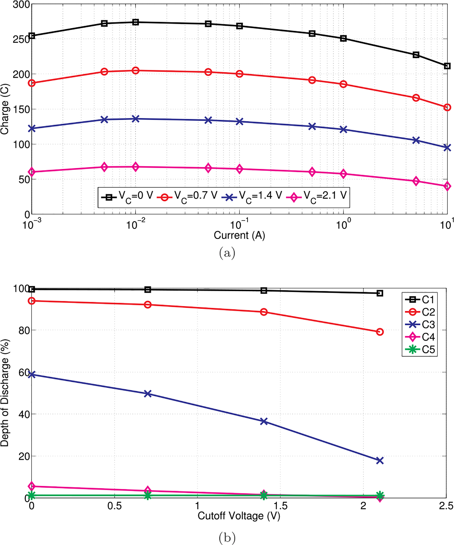
Simulation results using Fig. 7(a) with constant C₁ to explain observation 1. (a) Relationship between delivered charge and discharge current when initial voltage is 2.8 V and cutoff voltage (V_C) varies. (b) Effects of cutoff voltage on branch capacitor DOD when discharge current is 1 A.

5.4. Observation 3: for fixed voltage difference, Peukert constant decreases when initial voltage increases

While the first and second observations are explained by analyzing the model shown in Fig. 7(a) with the constant C₁, this section considers the third observation and utilizes both models because they lead to different Peukert constant patterns, as elaborated in Section 5.1. Specifically, the model shown in Fig. 7(b) with the variable C₁ results in a pattern consistent with the third observation: for a fixed voltage difference, the Peukert constant decreases when the initial voltage increases. On the other hand, the model shown in Fig. 7(a) with the constant C₁ results in an inconsistent pattern: the Peukert constants remain unchanged when the initial voltage varies. The difference between these two patterns is originated from the different assumptions on C₁ in these two models, as elaborated below.

For the voltage difference of 0.7 V, Fig. 11(a) plots the delivered charge results simulated using the model shown in Fig. 7(a). When the initial voltage varies from 2.8 to 0.7 V, the delivered charge associated with a particular discharge current is approximately equal for the current range of 10–0.01 A. When the discharge current is sufficiently low (i.e., 0.01–0.001 A), the delivered charge corresponding to a higher initial voltage is less. For example, when the discharge current is 0.001 A, the delivered charge decreases from 67.7 to 60.3 C when the initial voltage increases from 0.7 to 2.8 V. The physical mechanisms leading to this pattern have been elaborated in [31,32]. Specifically, when the discharge current is relatively high (i.e., 10–0.01 A), the energy loss due to self-discharge is negligible. For a fixed terminal voltage difference, the branch capacitor voltage difference is approximately equal when the initial voltage varies. Since all the five branch capacitors are constant, the delivered charge is also approximately equal. When the discharge current is sufficiently low (i.e., 0.01–0.001 A), the energy loss due to self-discharge is significant. For the same leakage resistor R₆, the leakage current is higher when the initial voltage is higher, which means that the energy loss is more significant and the delivered charge drops faster.

Fig. 11.

Simulation results using Fig. 7(a) with constant C₁ to explain observation 3. (a) Relationship between delivered charge and discharge current when voltage difference is 0.7 V and initial voltage (V_I) varies. (b) Effects of initial voltage on branch capacitor DOD when discharge current is 1 A.

The Peukert constants corresponding to Fig. 11(a) are listed in the row with ΔV = 0.7 V in Table 7: they are all 1.045 when the initial voltage varies from 0.7 to 2.8 V. When the discharge current is 1 A, the DOD results are plotted in Fig. 11(b). For all the five branch capacitors, the DOD remains almost constant when the initial voltage varies, which explains the flat Peukert constant pattern shown in Table 7.

On the other hand, Fig. 12(a) plots the delivered charge results simulated using the model shown in Fig. 7(b) with the variable C₁. The voltage difference is fixed at 0.7 V and the initial voltage varies from 2.8 to 0.7 V. Since C₁ is dependent on the voltage, the delivered charge associated with a particular discharge current increases when the initial voltage increases. The Peukert constants listed in Table 8 show the dependence on the initial voltage: it decreases from 1.060 to 1.036 when the initial voltage increases from 0.7 to 2.8 V. The DOD results are plotted in Fig. 12(b) when the discharge current is 1 A. Different from Fig. 11(b), the DOD for a specific branch capacitor increases when the initial voltage increases because the discharge time is longer. For example, the DOD for C₃ increases from 12.3 to 22.3% when the initial voltage increases form 0.7 to 2.8 V. In summary, consistent with the first and second observations, the branch capacitor DOD impacts the Peukert constant pattern shown in the third observation.

Fig. 12.

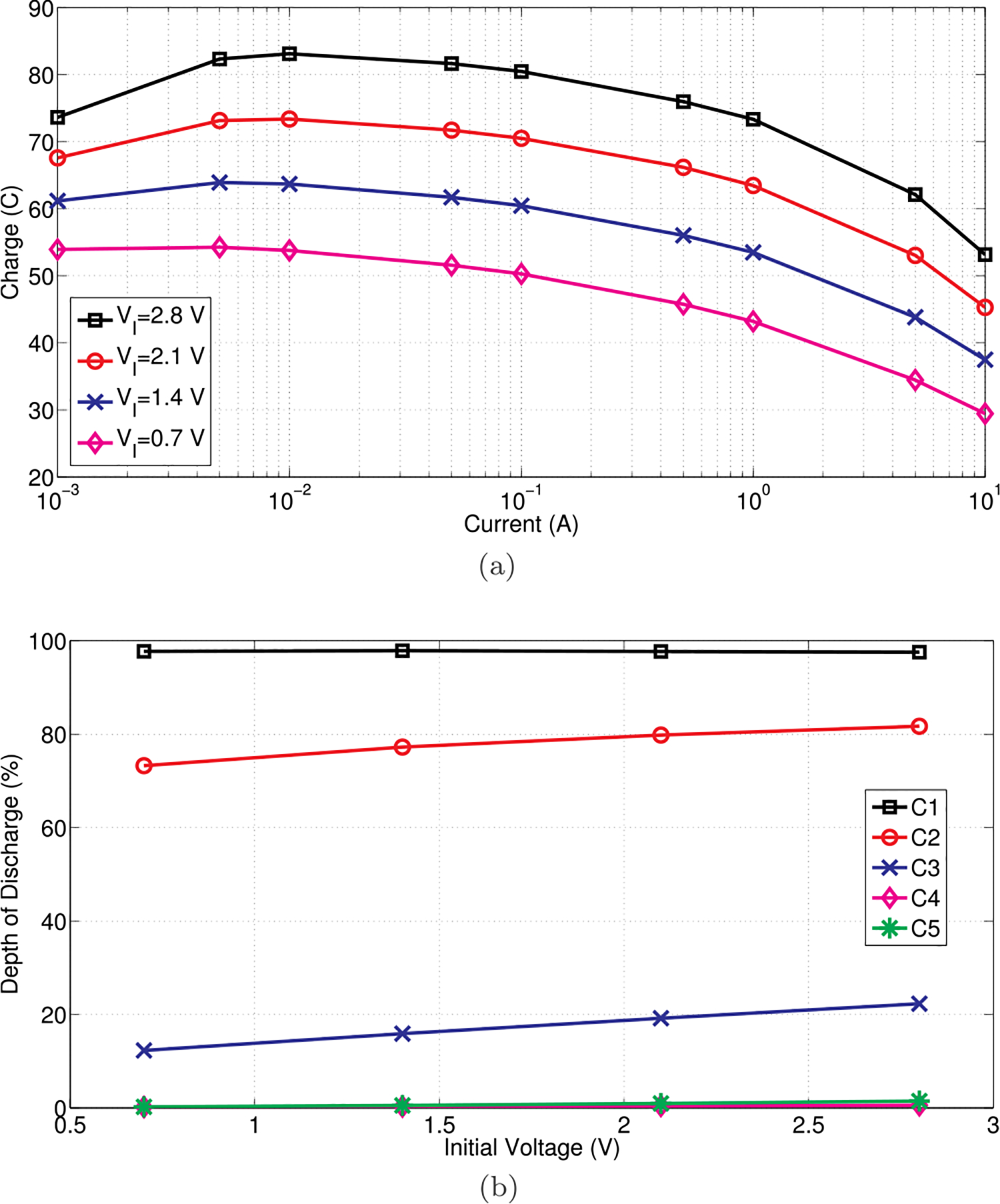
Simulation results using Fig. 7(b) with variable C₁ to explain observation 3. (a) Relationship between delivered charge and discharge current when voltage difference is 0.7 V and initial voltage (V_I) varies. (b) Effects of initial voltage on branch capacitor DOD when discharge current is 1 A.

6. Conclusion

This paper investigates the dependence of the supercapacitor Peukert constant on three voltage parameters of the constant current discharge process: initial voltage, cutoff voltage, and voltage difference. Three observations are made on the experimental results. First, for a fixed initial voltage, the Peukert constant decreases when the cutoff voltage decreases. Second, for a given cutoff voltage, the Peukert constant decreases when the initial voltage increases. Third, for the same voltage difference, the Peukert constant decreases when the initial voltage increases. To reveal the physical mechanisms accounting for these observations, two RC ladder circuit models are analyzed: one with a constant branch capacitor and the other with a voltage-dependent branch capacitor. Simulation results show that for the first and second observations, when the cutoff voltage is lower or the initial voltage is higher, the voltage difference is larger and more charge is released due to the charge-voltage relationship of capacitors. For the third observation, although the voltage difference is the same, more charge is delivered when the initial voltage is higher due to the voltage dependence of the supercapacitor capacitance. In these scenarios, the discharge time is longer, the branch capacitors are more deeply discharged and their DODs are higher, which makes them more responsive to the discharge current and ultimately leads to a smaller Peukert constant.

References

- [1].Yang H, A review of supercapacitor-based energy storage systems for microgrid applications, Proceedings of the 2018 IEEE Power & Energy Society General Meeting (PESGM 2018), (2018), pp. 1–5. [Google Scholar]
- [2].Pandolfo A, Hollenkamp A, Carbon properties and their role in supercapacitors, J. Power Source 157 (1) (2006) 11–27. [Google Scholar]
- [3].de Levie R, On porous electrodes in electrolyte solutions: I. Capacitance effects, Electrochim. Acta 8 (10) (1963) 751–780. [Google Scholar]
- [4].Yaniv M, Soffer A, The transient behavior of an ideally polarized porous carbon electrode at constant charging current, J. Electrochem. Soc 123 (4) (1976) 506–511. [Google Scholar]
- [5].Lai JS, Levy S, Rose MF, High energy density double-layer capacitors for energy storage applications, IEEE Aerosp. Electron. Syst. Mag 7 (4) (1992) 14–19. [Google Scholar]
- [6].Zubieta L, Bonert R, Characterization of double-layer capacitors for power electronics applications, IEEE Trans. Ind. Appl 36 (1) (2000) 199–205. [Google Scholar]
- [7].Ricketts B, Ton-That C, Self-discharge of carbon-based supercapacitors with organic electrolytes, J. Power Source 89 (1) (2000) 64–69. [Google Scholar]
- [8].Buller S, Karden E, Kok D, Doncker RWD, Modeling the dynamic behavior of supercapacitors using impedance spectroscopy, IEEE Trans. Ind. Appl 38 (6) (2002) 1622–1626. [Google Scholar]
- [9].Diab Y, Venet P, Gualous H, Rojat G, Self-discharge characterization and modeling of electrochemical capacitor used for power electronics applications, IEEE Trans. Power Electron 24 (2009) 510–517. [Google Scholar]
- [10].Sedlakova V, Sikula J, Majzner J, Sedlak P, Kuparowitz T, Buergler B, Vasina P, Supercapacitor equivalent electrical circuit model based on charges redistribution by diffusion, J. Power Source 286 (2015) 58–65. [Google Scholar]
- [11].Szewczyk A, Sikula J, Sedlakova V, Majzner J, Sedlak P, Kuparowitz T, Voltage dependence of supercapacitor capacitance, Metrol. Meas. Syst 23 (3) (2016) 403–411. [Google Scholar]
- [12].Rafik F, Gualous H, Gallay R, Crausaz A, Berthon A, Frequency, thermal and voltage supercapacitor characterization and modeling, J. Power Source 165 (2) (2007) 928–934. [Google Scholar]
- [13].Nadeau A, Hassanalieragh M, Sharma G, Soyata T, Energy awareness for supercapacitors using kalman filter state-of-charge tracking, J. Power Source 296 (2015) 383–391. [Google Scholar]
- [14].Zhang L, Wang Z, Sun F, Dorrell DG, Online parameter identification of ultracapacitor models using the extended kalman filter, Energies 7 (5) (2014) 3204–3217. [Google Scholar]
- [15].Reichbach N, Kuperman A, Recursive-least-squares-based real-time estimation of supercapacitor parameters, IEEE Trans. Energy Convers 31 (2) (2016) 810–812. [Google Scholar]
- [16].Chaoui H, Gualous H, Online lifetime estimation of supercapacitors, IEEE Trans. Power Electron 32 (9) (2017) 7199–7206. [Google Scholar]
- [17].Conway BE, Pell W, Liu T-C, Diagnostic analyses for mechanisms of self-discharge of electrochemical capacitors and batteries, J. Power Source 65 (1) (1997) 53–59. [Google Scholar]
- [18].Black J, Andreas HA, Effects of charge redistribution on self-discharge of electrochemical capacitors, Electrochim. Acta 54 (13) (2009) 3568–3574. [Google Scholar]
- [19].Kaus M, Kowal J, Sauer DU, Modelling the effects of charge redistribution during self-discharge of supercapacitors, Electrochim. Acta 55 (25) (2010) 7516–7523. [Google Scholar]
- [20].Kowal J, Avaroglu E, Chamekh F, Senfelds A, Thien T, Wijaya D, Sauer DU, Detailed analysis of the self-discharge of supercapacitors, J. Power Source 196 (1) (2011) 573–579. [Google Scholar]
- [21].Andreas HA, Black JM, Oickle AA, Self-discharge in manganese oxide electrochemical capacitor electrodes in aqueous electrolytes with comparisons to faradaic and charge redistribution models, Electrochim. Acta 140 (2014) 116–124. [Google Scholar]
- [22].Graydon JW, Panjehshahi M, Kirk DW, Charge redistribution and ionic mobility in the micropores of supercapacitors, J. Power Source 245 (2014) 822–829. [Google Scholar]
- [23].Yang H, Zhang Y, Power management in supercapacitor-based wireless sensor nodes, Supercapacitor Design and Applications, InTech, 2016, pp. 165–179. [Google Scholar]
- [24].Yang H, Analysis of supercapacitor charge redistribution through constant power experiments, Proceedings of the 2017 IEEE Power & Energy Society General Meeting (PESGM 2017), (2017), pp. 1–5. [Google Scholar]
- [25].Yang H, Bounds of supercapacitor open-circuit voltage change after constant power experiments, Proceedings of the 10th Electrical Energy Storage Applications and Technologies (EESAT 2017), (2017), pp. 1–5. [Google Scholar]
- [26].Yang H, Impact of charge redistribution on delivered energy of supercapacitors with constant power loads, Proceedings of the 2018 IEEE Applied Power Electronics Conference and Exposition (APEC 2018), (2018), pp. 2686–2690. [Google Scholar]
- [27].Yang H, Supercapacitor energy delivery capability during a constant power discharge process, Proceedings of the 44th Annual Conference of the IEEE Industrial Electronics Society (IECON 2018), (2018), pp. 1958–1963. [Google Scholar]
- [28].Yang H, Peukert’s law for supercapacitors with constant power loads: applicability and application, IEEE Trans. Ind. Appl 55 (4) (2019) 4064–4072. [DOI] [PMC free article] [PubMed] [Google Scholar]
- [29].Yang H, A revisit to supercapacitor capacitance measurement method 1A of IEC 62391–1, Proceedings of the 2018 IEEE Energy Conversion Congress and Exposition (ECCE 2018), (2018), pp. 2478–2482. [Google Scholar]
- [30].Yang H, Evaluation of cell balancing circuits for supercapacitor-based energy storage systems, Proceedings of the 2019 IEEE Transportation Electrification Conference and Exposition (ITEC 2019), (2019), pp. 1–5. [Google Scholar]
- [31].Yang H, Estimation of supercapacitor charge capacity bounds considering charge redistribution, IEEE Trans. Power Electron 33 (8) (2018) 6980–6993. [DOI] [PMC free article] [PubMed] [Google Scholar]
- [32].Yang H, Effects of supercapacitor physics on its charge capacity, IEEE Trans. Power Electron 34 (1) (2019) 646–658. [DOI] [PMC free article] [PubMed] [Google Scholar]
- [33].Doerffel D, Sharkh SA, A critical review of using the peukert equation for determining the remaining capacity of lead-acid and lithium-ion batteries, J. Power Source 155 (2) (2006) 395–400. [Google Scholar]
- [34].Griffith LD, Sleightholme AE, Mansfield JF, Siegel DJ, Monroe CW, Correlating Li/O2 cell capacity and product morphology with discharge current, ACS Appl. Mater. Interf 7 (14) (2015) 7670–7678. [DOI] [PubMed] [Google Scholar]
- [35].Hausmann A, Depcik C, Expanding the Peukert equation for battery capacity modeling through inclusion of a temperature dependency, J, Power Source. 235 (2013) 148–158. [Google Scholar]
- [36].Mills EM, Kim S, Determination of Peukert’s constant using impedance spectroscopy: application to supercapacitors, J. Phys. Chem. Lett 7 (24) (2016) 5101–5104. [DOI] [PubMed] [Google Scholar]
- [37].Zhu J, Xu Y, Enhanced electrochemical performance of polypyrrole depending on morphology and structure optimization by reduced graphene oxide as support frameworks, Electrochim. Acta 265 (2018) 47–55. [Google Scholar]
- [38].Campillo-Robles J, Artetxe X, del Teso Sanchez K, Gutierrez C, Macicior H, Roser S, Wagner R, Winter M, General hybrid asymmetric capacitor model: validation with a commercial lithium ion capacitor, J. Power Source 425 (2019) 110–120. [Google Scholar]
- [39].Yang H, A study of Peukert’s law for supercapacitor discharge time prediction, Proceedings of the 2018 IEEE Power & Energy Society General Meeting (PESGM 2018), (2018), pp. 1–5. [Google Scholar]
- [40].Yang H, Prediction of supercapacitor discharge time using Peukert’s law, Proceedings of the 2019 IEEE Power & Energy Society General Meeting (PESGM 2019), (2019), pp. 1–5. [Google Scholar]
- [41].Yang H, Application of Peukert’s law in supercapacitor discharge time prediction, J. Energy Storage 22 (2019) 98–105. [DOI] [PMC free article] [PubMed] [Google Scholar]
- [42].Yang H, Dependence of supercapacitor Peukert constant on voltage, aging, and temperature, IEEE Trans. Power Electron 34 (10) (2019) 9978–9992. [DOI] [PMC free article] [PubMed] [Google Scholar]
- [43].Eaton, HV series supercapacitors datasheet, http://www.cooperindustries.com/content/dam/public/bussmann/Electronics/Resources/product-datasheets/Bus_Elx_DS_4376_HV_Series.pdf.
- [44].AVX, SCC series supercapacitors datasheet, http://datasheets.avx.com/AVX-SCC.pdf.
- [45].Maxwell, BC series supercapacitors datasheet. http://www.maxwell.com/images/documents/bcseries_ds_1017105-4.pdf.