Automatic segmentation of brain tumor resections in intraoperative ultrasound images using U-Net

Abstract.

To compensate for the intraoperative brain tissue deformation, computer-assisted intervention methods have been used to register preoperative magnetic resonance images with intraoperative images. In order to model the deformation due to tissue resection, the resection cavity needs to be segmented in intraoperative images. We present an automatic method to segment the resection cavity in intraoperative ultrasound (iUS) images. We trained and evaluated two-dimensional (2-D) and three-dimensional (3-D) U-Net networks on two datasets of 37 and 13 cases that contain images acquired from different ultrasound systems. The best overall performing method was the 3-D network, which resulted in a 0.72 mean and 0.88 median Dice score over the whole dataset. The 2-D network also had good results with less computation time, with a median Dice score over 0.8. We also evaluated the sensitivity of network performance to training and testing with images from different ultrasound systems and image field of view. In this application, we found specialized networks to be more accurate for processing similar images than a general network trained with all the data. Overall, promising results were obtained for both datasets using specialized networks. This motivates further studies with additional clinical data, to enable training and validation of a clinically viable deep-learning model for automated delineation of the tumor resection cavity in iUS images.

1. Introduction

1.1. Background

In brain tumor surgery, preoperative magnetic resonance (MR) images provide essential information, such as the location of the tumor. Because of the tissue deformation in the operating room, nonrigid registration of the preoperative MR (pMR) with intraoperative data has been widely studied.^1,2 In particular, several works used intraoperative ultrasound (iUS) to register the pMR.^3–8 A MICCAI 2018 Challenge was also organized on this topic.⁹ However, few methods^10,11 addressed the intraoperative deformation due to tissue resection. In order to model tissue removal accurately, the location of the removed tissue needs to be determined. One approach is to acquire intraoperative images of the resection cavity and segment the removed tissue.

We recently proposed a biomechanical model-based registration framework using iUS acquisitions.⁴ One of the requirements for the method was its usability in a clinical setting. In particular, integration with the clinical workflow, minimal user interaction, and execution time in the operating room were taken into consideration. Currently, our method does not model the resection cavity. To integrate tissue resection in the model, the removed tissue needs to be localized. This information can be obtained from the iUS B-mode images, through manual segmentation. However, manual segmentation is time consuming and error-prone, especially in ultrasound images. Also, user input needs to be minimal in the operating room. Thus, an automatic segmentation method for the resection cavity in iUS images would be highly beneficial. This is a difficult task because of the high variability in the location of the cavity as well as image quality and features.

Automatic segmentation of the resection cavity has several uses in image-guided brain tumor resection surgery. First, the volume and precise delineation of the removed tissue can be used to account for tissue removal in the registration process. After the resection procedure has started, tissue removal is an additional source of deformation that should be taken into account. Also, the resection cavity in the registered pMR can be updated with a realistic signal in the visualization system.

Moreover, the segmentation of the resection cavity can be used along with a segmentation of the tumor to assess whether the resection is complete. The tumor can be delineated manually or automatically in the pMR, and its segmentation can be registered along with the pMR to the iUS volume. Or, although a challenging task, the tumor could be directly segmented in the iUS volume. The resulting tumor segmentation can then be compared with the resection cavity segmentation to evaluate the progression of the procedure.

1.2. Contributions

In this work, we present an evaluation of deep learning-based methods to automatically segment the resection cavity in iUS images. To do this, we created ground truth (GT) segmentations and validated them with a clinical expert. We trained several two- (2-D) and three-dimensional (3-D) segmentation neural networks and compared the corresponding results. Preliminary results have been presented recently at the 2019 SPIE conference.¹² Unlike that study where only 2-D networks were evaluated, herein we also implement a 3-D network and compare it with the 2-D networks. Further, we evaluate the robustness of the networks to different datasets by evaluating our networks on two datasets with different acquisition parameters and using cross-validation on multiple folds.

2. Related Work

2.1. Deep Learning in Ultrasound

Deep learning has become one of the most commonly used methods for image processing tasks, such as classification or segmentation. The use of deep learning for medical image analysis has recently been reviewed by Litjens et al.¹³ Deep learning techniques have been successfully applied to ultrasound images in several applications, such as the diagnosis of medical conditions,^14–19 segmentation,^19,20 image registration,^21,22 and reconstruction.²³

Many applications need to segment ultrasound images.^19,20,24,25 In particular, several works segmented structures in brain iUS images: midbrain,²⁶ falx and sulci,^8,27 and tumor.²⁸ A recent work proposed an automated segmentation method for the resection cavity in postoperative MR.²⁹ However, to the best of our knowledge, no method has been proposed to segment the resection cavity in iUS images. Most deep learning segmentation methods use a network based on U-Net with an encoder and a decoder path.³⁰

For 3-D datasets, there are several options to process the volumes. The volumes can be processed slice by slice by a 2-D network or directly using a 3-D network. The advantages of 2-D networks are that they use less memory and are faster. In particular, entire slices can usually be processed with no or little resizing. Whereas with a 3-D network, smaller input sizes are used due to memory constraints and a sliding window (SW) is used. On the other hand, the advantage of 3-D networks is the use of spatial context in all planes. Spatial 3-D context is important for segmentation tasks and can significantly improve results.³¹

A compromise can be found using several slices with a 2-D network (2.5D). Each group of slices is composed of either adjacent slices^32,33 or slices from different planes.^26,34 Some methods include another network to combine the outputs of two 2-D networks in different planes.^34,35

Some studies circumvented the 3-D network limitations with various workarounds. Pedemonte et al.³⁶ suggested that using wider input sizes (e.g., $256\times 256\times 32$) was more performant than cubic patches with the same size in memory (e.g., $128\times 128\times 128$). This allowed a larger context in two directions while retaining some context in the third plane. Roth et al.³⁷ trained 3-D networks at different scale levels. Segmentations were estimated for each scale level, starting at the lowest resolution. At each level, the input consisted of both the volume to segment and the segmentation estimated at the previous level. With this method, the final segmentations were estimated at the original scale without using an SW. Liu et al.³⁸ transferred weights from a 2-D network to a 3-D network. A 2-D segmentation network is first trained with 2-D slices. Then, the weights in the encoding path of the 2-D network are transferred to the 3-D network. The decoding path of the 3-D network is then trained. This method allowed a better training of the 3-D network.

2.2. Registration of Brain pMR and iUS

In brain surgery, tissue deformation occurs in the operating room due to several causes including the surgeon’s actions and tissue resection. As such, methods to compensate the deformation and register the pMR with intraoperative data have been studied.^1,2 Some methods that establish correspondences between the pMR and iUS are established using similarity metrics^3,5 or feature descriptors.⁶ Other methods use a biomechanical model of the brain,^10,11,39,40 where the deformation is estimated by solving correspondence constraints with the finite element method.

The deformation due to tissue resection is significant. In both intensity-based methods and model-based methods, the location of the resection cavity can be used to improve the results. To localize the resection cavity, some methods used manual or semiautomatic segmentation methods that required user input.^39,40 Bucki et al.¹⁰ used an automatic ellipsoid estimation of the cavity, and Fan et al.¹¹ proposed an automatic estimation method based on stereo cameras. However, the shape of the resection cavity can be complex and may not be estimated correctly with only surface data. On the other hand, iUS provides subsurface information and iUS volumes can be acquired so that the volume contains the whole cavity. An automatic segmentation of the resection cavity in iUS images would enable accurate identification of the resection cavity nodes in registration models.

3. Methods

3.1. Dataset

In this work, we used the volumes from two publicly available databases, RESECT⁴¹ and BITE.⁴² The RESECT dataset contains 23 cases, for which pMR and iUS volumes are available. For each case, one iUS volume was acquired before, during, and after resection. In this study, we used the volumes acquired during and after resection. The iUS volumes were acquired using two types of linear probes (12FLA-L and 12FLA, with a frequency range of 6 to 12 MHz and a footprint of $48\times 13\mathrm{mm}$ and $32\times 11\mathrm{mm}$, respectively). The volume sizes range from 221 to 492 voxels (with a mean of 347). The volumes are isotropic and the mean voxel size is 0.21 mm (range 0.14 to 0.36). Each iUS volume was acquired such as the complete resection cavity is contained in the volume. In the following, we refer to individual cases by their number in the database followed by “a” or “d” for after or during.

In RESECT, the volumes acquired during and after resection are different because they are acquired at different timepoints. Unlike the images after resection, the images during resection contain tumor tissue, and the resection cavity is smaller. A Wilcoxon signed-rank test on the paired during and after volumes showed statistical difference of the volumes of the GT resection cavity ($p$-value of 9.155e-05). Because of this difference, we ensured an equal repartition of the timesteps when splitting the dataset, to keep the folds representative of the whole dataset.

The BITE dataset contains pre- and postresection MR and US volumes for 14 patients. Multiple iUS volumes were acquired for each patient, and each was assigned a letter from $u$ to $z$, appended to the patient number. Postresection iUS was available for 13 of the patients. The ultrasound probe was a P7-4 MHz phased array transducer. The volumes sizes range from 159 to 516 voxels (with a mean of 316). The volumes are isotropic and the voxel size is 0.3 mm for all volumes. Each iUS volume does not cover the complete resection cavity, but several volumes were acquired with different angles to cover as much anatomy as possible.

The acquisition protocols in the two dataset are different, not only in the imaging devices but also in the operative strategy.

3.2. Ground Truth Creation

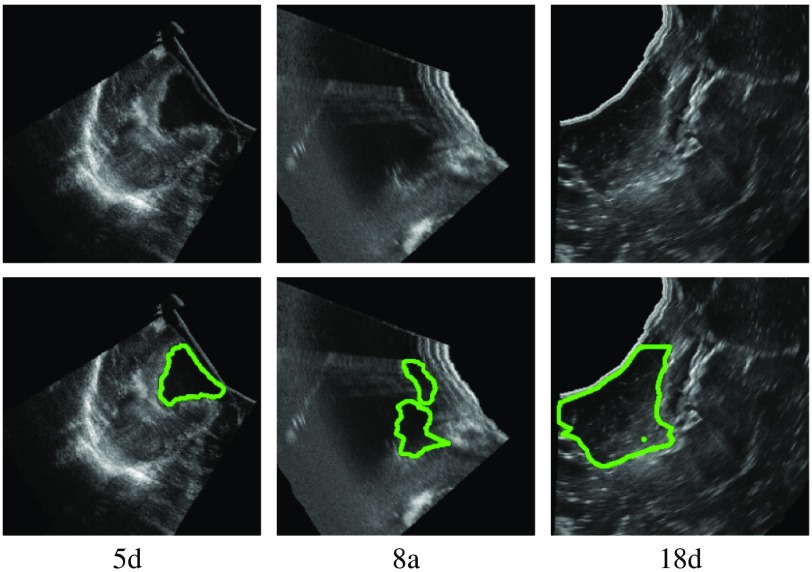
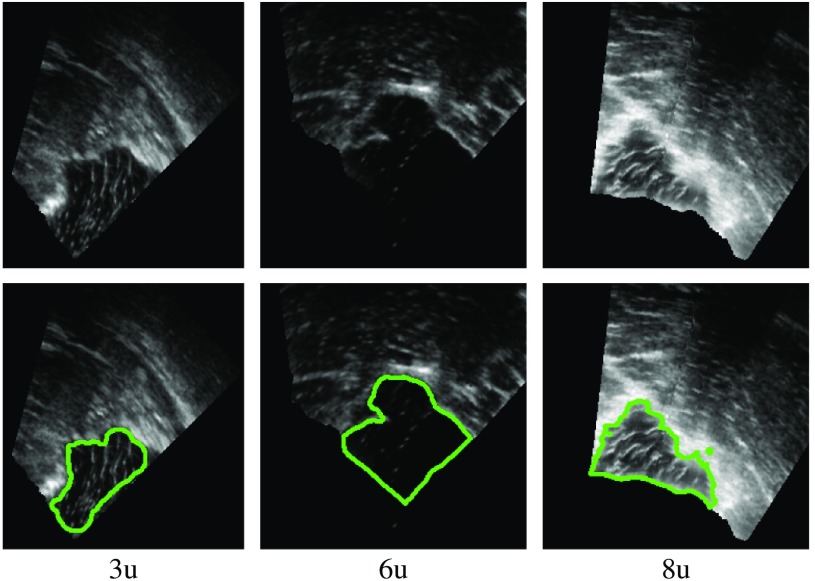
We manually created GT segmentations for the RESECT and BITE datasets. The two first authors of this paper created the segmentations. Since they are not experts in radiology, all segmentations were reviewed and revised by a clinical expert (third author). We segmented 37 RESECT volumes and 13 BITE volumes. Figures 1 and 2 show examples of GT segmentations for both datasets.

Fig. 1.

Example of GT segmentations (RESECT).

Fig. 2.

Example of GT segmentations (BITE).

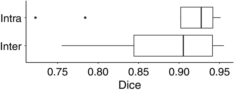
For RESECT volumes, observer 1 segmented 37 volumes (21 after resection, 16 during). These are the volumes in which the resection cavity is visible and possible to segment, which was the case in most of the available volumes. We then evaluated the intrarater and interrater variability on 10 cases, where observer 1 created a second segmentation and observer 2 created one. The overall intra- and interrater variability results are shown in boxplots in Fig. 3. In each boxplot in this and in the remaining figures in this paper, the line inside boxes indicates the median. The box hinges represent the first and third quartiles. The whiskers extend from the hinges to the value no further than 1.5 times the interquartile range from the hinge. Overall, there was a high agreement between the segmentations, with a mean Dice score (DSC) of 0.89 for both interrater and intrarater comparisons. However, several areas in the iUS volumes were difficult to interpret, leading to interrater differences. The segmentations were then reviewed by the two observers as well as a clinical expert (third author). For each case, the original segmentation was edited if needed, according to the expert’s directions. For cases segmented by the two observers, the best segmentation was selected using the expert’s comments. These final segmentations were used for the GT to compare with the segmentations estimated by the trained models.

Fig. 3.

Interrater and intrarater Dice scores.

For the BITE dataset, observer 1 segmented seven cases and observer 2 segmented six cases. The segmentations were reviewed by the two observers and edited if needed to create GT segmentations.

3.3. Network Architecture

We implement 2-D and 3-D versions of the U-Net network proposed by Ronneberger et al.³⁰ We compare three different architectures (Fig. 4):

Fig. 4.

Schematic of the three U-Net models.

• •a 2-D network with one input slice (2D-1),
• •a 2-D network with seven input slices (2D-7),
• •a 3-D network (3D).

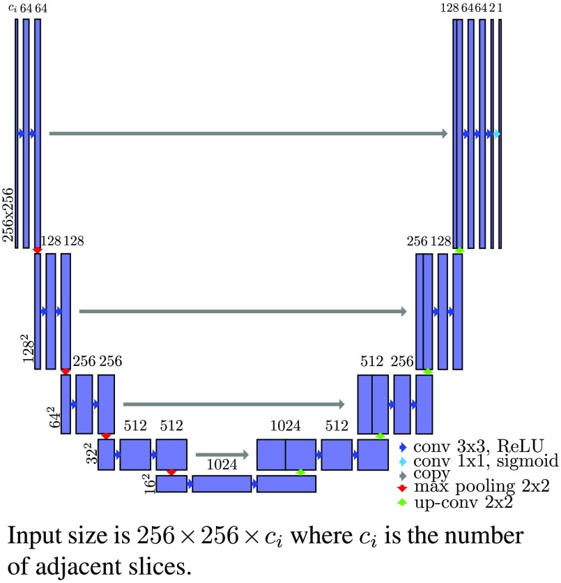
First, we test a 2-D version with an input size of $256\times 256$. The layer architecture is shown in Fig. 5. The differences from the original U-Net are the layer sizes, the use of padded convolutions, and a sigmoid function instead of a soft-max in the last layer.

Fig. 5.

Schema of the 2-D U-Net architecture.

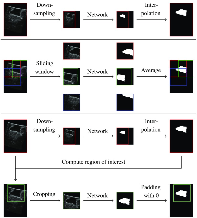
To train the network, the training volumes are cropped to the network’s input size. For testing, we compare three sampling methods:

• •downsampling (DS),
• •using an SW,
• •using the estimated segmentation from the DS method to compute a region of interest (ROI) and crop the volumes to that region.

Figure 6 shows a schematic of the three methods. With the DS method, the original volumes are downsampled using a linear interpolation, and the estimated segmentations are upsampled using the nearest neighbors algorithm. The SW approach consists of evaluating the network on several $256\times 256$ patches extracted from the original volumes, with a stride (distance between patches) of 64 pixels. The resulting segmentation patches are then combined using a per-pixel average over the patches. The ROI method uses the segmentation estimated with the DS method to compute a region of interest (bounding box of the segmentation). The network is then evaluated on the original volume cropped to the bounding box.

Fig. 6.

Schematic of the three sampling methods.

The volumes are processed slice by slice in one direction. To assess the impact of context on the segmentation, we train two networks 2D-1 and 2D-7 with one and seven input slices, respectively. The slices are grouped along the feature axis of the input layer.

We also implement a 3-D version in which the input consists of $128\times 128\times 128$ 3-D patches. For both training and testing, a 3-D SW is used to extract patches. For training, the patches are only extracted with a stride of 32 voxels, from a $256\times 256\times 256$ bounding box containing the resection cavity, to decrease the number of background-only patches. For testing, the SW covers the whole volumes, with a stride of 64 voxels.

3.4. Pre- and Postprocessing

In a preprocessing step, the volumes are normalized by subtracting the mean volume intensity value and then dividing by the standard deviation. This step is run just before volume sampling (and after data augmentation in the training phase).

All cases were postprocessed by converting the output of the networks to binary masks with a threshold of 0.5 and then selecting the largest connected component.

3.5. Training

The models were trained using the Adam optimizer⁴³ with ${\beta }_1=0.9$, ${\beta }_2=0.999$, and a learning rate of ${10}^{-5}$. The 2-D models were trained for 100 epochs and the 3-D models for 20 epochs. We selected the weights of the best epoch for testing, minimizing the loss over the training and validation sets. With the Dice loss, the training process was very stable, with the loss generally decreasing (not increasing substantially) over time. Thus, the epoch selection process was straightforward. Among the training cases, four (RESECT) or one (BITE) were selected randomly as validation cases for monitoring and epoch selection purposes.

We tried three loss functions and eventually used the Dice loss function as suggested in Ref. 44. The other two had issues due to class imbalance, as around 95% of the voxels were background. With the binary cross-entropy loss function [Eq. (1)], training the models was difficult and often resulted in empty (all background) estimations. Of nine training processes with this loss function, three did not converge and produced all background outputs. We then tried to weight the two classes using a lower weight $w_b$ for the background voxels than for the foreground voxels $w_f=1-w_b$ [Eq. (2)]. This solved the convergence issue, however, the lower weight for background voxels tended to increase false positives (FPs). The FP ratio (number of FP voxels over the total number of voxels) mean was 0.6% with equal weights and 1.1% with a lower weight $w_b=0.25$ for the background. This increase of FP voxels was observed with $w_b=0.25$ and $w_b=0.05$. The Dice loss function [Eq. (3)] did not have these issues: the training always converged and the models achieved better results. In particular, the number of FP was lower: the mean FP ratio was 0.06%. Thus, we chose the Dice loss function to train the models presented in this work:

$$l(y_t,y_p)=-\sum _i{y}_t[i]\log y_p[i]+(1-y_t[i])\log (1-y_p[i]),$$ (1)

$$l(y_t,y_p)=-\sum _i{w}_f{y}_t[i]\log y_p[i]+w_b(1-y_t[i])\log (1-y_p[i]),$$ (2)

$$l(y_t,y_p)=1-\frac{2\sum _i{y}_t[i]y_p[i]+ϵ}{\sum _i{y}_t[i]+\sum _i{y}_p[i]+ϵ}.$$ (3)

We augmented the data during the training process using random transformations. At the beginning of each epoch, each original volume was transformed with the following transformations with a probability of 0.5 for each transformation:

• •affine transformation, with a translation in a random direction and a distance up to 16 voxels (around 3.2 mm), and a rotation around a random axis and angle between $-10\mathrm{deg}$ and 10 deg;
• •grid deformation, where a $32\times 32\times 32$ grid is randomly deformed using a normal distribution, and the original volume is interpolated using the nearest neighbors;
• •scale, using a random scale factor between 0.75 and 1.25.

The data augmentation prevented overfitting to the training data: without using data augmentation, the validation loss would start increasing after a few iterations indicating that the model overfitted. With the augmentation process, this was prevented, and the validation loss would not increase substantially over time.

3.6. Training Strategies

The networks were first trained and evaluated on a single dataset. Then, to evaluate robustness of networks trained using one dataset when applied to another, we evaluated on BITE cases the networks trained on the RESECT database without retraining them. We also tested fine tuning strategies by training three additional networks:

• 1.Fine tuning the network trained on RESECT with BITE cases;
• 2.Training a network only with BITE cases (from scratch);
• 3.Fine tuning the network trained on BITE (2) with RESECT cases.

The models were evaluated on four folds with 10 test cases each for RESECT and two folds with four test cases each for BITE. The folds were chosen by randomly assigning test volumes for each fold, at a volume level so that all slices and/or patches from the same volume are in one set. In each fold, the ratio of cases after resection versus during resection was kept.

Finally, we trained a network with cases from both RESECT and BITE. Because there are more RESECT cases than BITE cases, we generated several augmentations for each BITE case in the training set to ensure an equal number of cases from each dataset. This was to prevent the training to favor features from the dataset with more cases. This model was evaluated on one fold with 14 test volumes (10 RESECT volumes and 4 BITE volumes).

3.7. Validation Studies

First, we compare the three sampling methods for the 2-D networks (DS, SW, ROI). The study is based on the results of the 2D-1 and 2D-7 networks on the RESECT volumes (four folds). Then, we evaluate the three network architectures (2D-1, 2D-7, 3D) based on the results on the RESECT volumes. Finally, we analyze the results on RESECT and BITE, with the networks trained from scratch, fine tuned, and trained on both datasets.

The evaluation metrics reported such as Dice scores are computed on the whole volumes. In the following, we define a failed case as a case with a Dice score lower than 0.5, as opposed to a case successfully segmented. To the best of our knowledge, no other method has been proposed for the segmentation of the cavity in iUS images. As such, no comparison with other results is possible.

4. Results and Discussion

4.1. Comparison of Sampling Methods

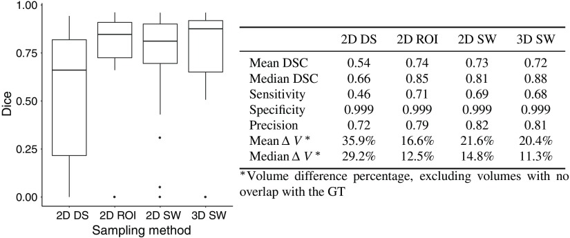
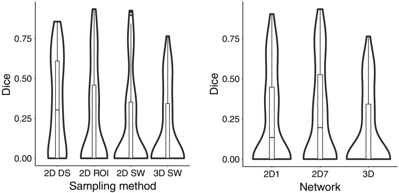
We compared three sampling methods for the 2-D networks. Figure 7 gives an overview of the scores for each sampling methods.

Fig. 7.

Comparison of the sampling methods (RESECT); the results are computed with the test sets of each fold.

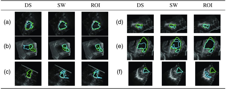
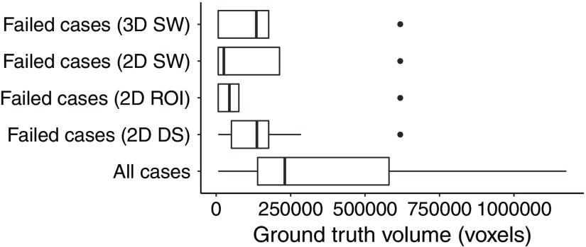
The DS method performed worse than the SW and the ROI methods. There were cases for which the cavity was only partially or overly segmented [Figs. 8(a) and 8(b)]. With the DS method, there were 11 out of 37 cases with no overlap with the GT [Fig. 8(c)]. The SW and ROI method only had four such cases. These cases had resection cavity volumes among the smallest in the dataset: all but two of these volumes were smaller than the median volume (Fig. 9). The errors were likely due to the DS, which reduced the size of the cavity.

Fig. 8.

Example of differences between sampling methods (green: GT; blue: estimation).

Fig. 9.

Comparison of the GT volumes in all and failed cases.

In a few cases, the ROI method performed better than the SW and did not have patch errors [Figs. 8(d) and 8(e)]. The ROI approach also had more successful cases than the SW. However, the SW method had fewer segmentations with no overlap with the GT [Fig. 8(f)]. The SW method may be more reliable than the ROI method since it does not depend on the downsampled ROI estimation and the SW covers the whole volume. Estimating the segmentation for one case took longer with the SW (around 1 min on a NVIDIA^® GeForce GTX TITAN X) than the DS and ROI methods (around 15 s) due to the evaluation of several patches. Depending on accuracy and time constraints, the SW or the ROI may be favored over the other.

4.2. Comparison of Network Architectures

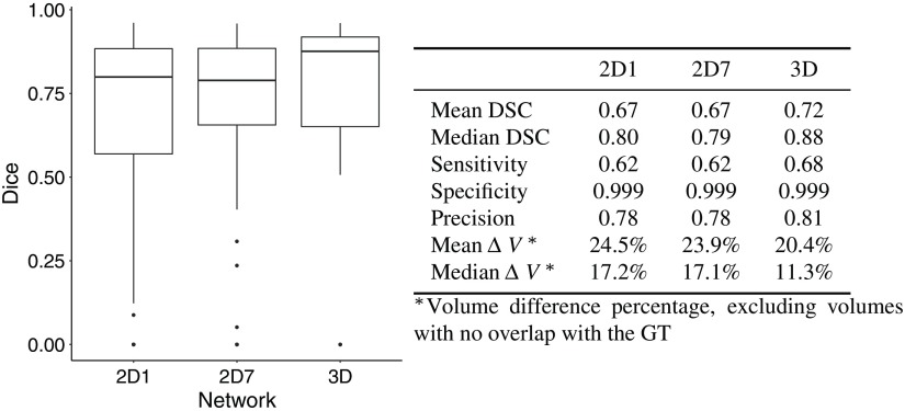
The 2-D network with seven input slices (2D-7) performed slightly better than the one with only one input slice (2D-1) when using the DS method. The segmentations were improved in areas where the cavity was not detected: at the boundaries and where other components such as blood altered the iUS signal. With the SW and ROI approaches, the differences were minimal. Overall, the 3-D network performed better, as the segmentations produced by the 3-D network had greater overlap with the GT. However, the runtime was longer due to a large number of patches to process: the average runtime for one case was 5 min (1.5 s per patch). 2-D networks might be preferred in clinical application because of their shorter runtime. Figure 10 presents the Dice scores for all architectures.

Fig. 10.

Comparison of the network architectures (RESECT); the results are computed with the test sets of each fold.

4.3. Evaluation on a Single Dataset

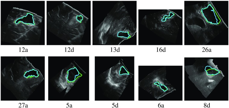
We first discuss the results obtained by training and evaluating on the RESECT dataset only. Figure 11 shows examples of results for one fold with the 3-D network. In the successful cases, the estimated segmentations were very similar to the GT. With the best performing method (3-D network), the mean Dice score was 0.72 over the whole dataset, and the median was 0.88. Very noisy areas (such as case 8d in Fig. 11) were successfully segmented. In cases with other cavities (such as the ventricle in case 26a), the resection cavity was selected.

Fig. 11.

Example of RESECT segmentations for one fold with the 3-D network (green: GT; blue: estimation).

There were four cases with no overlap with the GT (5d, 14d, 15a, and 18d). In cases 14d and 15a, the resection cavity was very small and thus difficult to locate. The DS method was the most sensitive to small volumes. Case 5d has a large area with a high-intensity signal (Fig. 1). In case 18d, the signal in the bottom resection cavity is different from the other cases. We expect that larger training dataset would improve the training and such errors would be avoided.

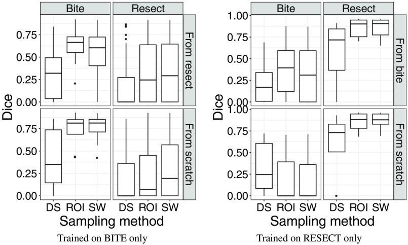
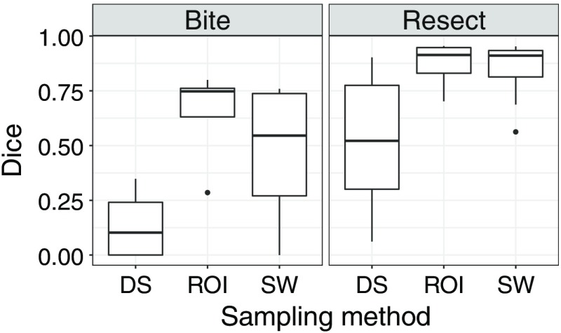
The results were similar for the BITE dataset. The mean Dice score was 0.75 and the median 0.81. The Dice scores are shown in the bottom left plot in Fig. 12. There was no failed case with the SW and ROI methods, and only one with the DS method.

Fig. 12.

Comparison of Dice scores with different training initialisations; the results are computed with the test sets for each fold (when testing on the same dataset the network was trained with) or all cases (otherwise).

4.4. Evaluation on Both Datasets Without Fine-Tuning

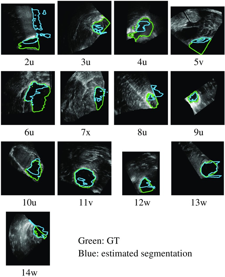
We evaluated the networks, trained with only RESECT cases and without retraining, on the BITE dataset. The networks did not have as good results on BITE cases. Some cases were successfully segmented; however, there were more failed cases than with RESECT. Figure 13 shows the estimated segmentations with the 2D-7 network. Overall, the DS method performed better than the other sampling methods and had fewer incorrect segmentations. Some of the estimated segmentations included out-of-field voxels and could be refined using a mask during postprocessing. Figure 14 presents the Dice scores obtained with all the networks in a boxplot along with estimated densities.

Fig. 13.

Example of BITE segmentations with the 2D-7 network trained with only RESECT cases (green: GT; blue: estimation).

Fig. 14.

Dice scores for the BITE datasets (network only trained with RESECT cases); the results are computed with all BITE cases.

The obtained results are promising given that the training process did not include any volume from the BITE dataset. The failed cases were cases for which the probe was inserted into the resection cavity and only part of the cavity is visible in the volumes (cases 5v, 7x, and 14v). This is different from the RESECT database, in which all volumes contain the complete resection cavity. This is due to different acquisition protocols. In RESECT, linear probes were used to acquire the entire resection cavity from the cortical surface. In BITE, smaller probes with a lower frequency were used within the cavity. As such, only part of the cavity was visible in the acquired volumes. With this difference in the cavity between the two datasets, it is not surprising that networks trained with one dataset do not generalize well to another dataset, and dataset-specific training leads to better results. For datasets with similar probe types and acquisition protocols, we expect that training on one dataset could generalize well on another.

4.5. Evaluation on Both Datasets With Fine-Tuning

Figure 12 shows the results obtained with the four networks, trained on BITE or RESECT and with or without fine-tuning. On each plot, the rows represent a different network: on the bottom row, the network was trained from scratch, whereas on the top row, the training was initialized using the weights of the network trained with the other datasets. Each network was tested on the two datasets, using the test split for the dataset the network was trained with, and all cases for the other dataset. The test results are presented in different columns for each dataset. The results were always better for the dataset the networks were last trained with. The networks performed poorly on the other dataset, with the fine-tuned networks having slightly better results. The fact that the models only had good results on one dataset is probably due to the difference between the two datasets of the resection cavity being complete or not. Because of that, training a network to perform well for the two datasets appears to be very difficult.

4.6. Evaluation on Both Datasets With Training on Both Datasets

Figure 15 shows the results for one network trained with cases from RESECT and BITE. Despite having an equal number of cases from each dataset in the training set, the network had better results on RESECT cases. This confirms that training a specific model for each dataset is better.

Fig. 15.

Comparison of Dice scores (network trained with both RESECT and BITE cases); the results are computed with the test set, which includes RESECT and BITE cases.

5. Impact on Interventional and Surgical Data Science

With the advent of deep learning in medical image analysis, opportunities have arisen in many applications to use data collected from populations of patients to create neural networks that assist with difficult interventional tasks. Image-guided brain tumor resection surgery is an example of such an application. Ultrasound imaging is widely used to locate subsurface anatomical structures as they deform during the surgery. However, these images are very noisy and difficult to interpret, and effective automated analysis methods have remained elusive. One approach for assisting the surgeons in interpreting the ultrasound is by registering the pMR to it using biomechanical models. Such models need the region of resection, which can be obtainable from the ultrasound, as input. Our goal in this work is to leverage large datasets and deep learning techniques to segment the resection cavity to create such data-driven models. Our approach is applicable to any surgical intervention where resection is being performed and registration of preoperative imaging to intraoperative imaging is beneficial. For example, thorascopic or cardiovascular interventions could benefit from automated analysis provided by data-driven models.

6. Conclusions

This is the first work in which an automatic method has been proposed for segmenting the resection cavity in ultrasound images for brain tumor resection surgery. To validate our technique, we created GT segmentations of the resection cavity for the volumes in the RESECT and BITE databases. Using these data, we trained 2-D and 3-D neural networks to segment the resection cavity in iUS volumes of the brain. We found that 3-D networks performed better than 2-D networks; however, 2-D networks had good results with smaller execution times. Depending on the time and accuracy constraints in the operating room, 2-D or 3-D may be preferred. We compared several sampling methods and also evaluated the generalizability of the networks using two datasets. There was a high variance between the two datasets, in particular, the cavity was only partially visible in many BITE volumes. In this case, we showed that training specific networks is better.

In future work, the use of the pMR as an additional network input can be investigated. While the pMR and iUS do not fully match because of the brain-shift, the network could still benefit from this additional information.

The datasets available are relatively small for deep learning applications, and we expect that larger datasets would improve the training of the networks. While larger datasets would provide a better validation of the discussion, promising results were obtained despite the small dataset size and the low quality of iUS images. The resulting segmentations are accurate enough to be used in pMR-iUS registration to take the resection cavity and the associated discontinuity into account. These promising results motivate further research with a larger dataset.

Further, this work demonstrates that deep learning can be successfully applied to ultrasound segmentation even with relatively small datasets. It completes previous evaluations of deep learning methods on the RESECT and BITE datasets.^7,8 Ultrasound images are difficult to segment because of the high variability and the low quality of the images. And thus, deep learning methods could provide a major impact on the field of data-driven computer-assisted surgery.

Biography

Biographies of the authors are not available.

Disclosures

The authors declare that there is no conflict of interest.

References

- 1.Gerard I. J., et al. , “Brain shift in neuronavigation of brain tumors: a review,” Med. Image Anal. 35, 403–420 (2017). 10.1016/j.media.2016.08.007 [DOI] [PubMed] [Google Scholar]
- 2.Bayer S., et al. , “Intraoperative imaging modalities and compensation for brain shift in tumor resection surgery,” Int. J. Biomed. Imaging 2017, 1–18 (2017). 10.1155/2017/6028645 [DOI] [PMC free article] [PubMed] [Google Scholar]
- 3.Riva M., et al. , “3D intra-operative ultrasound and MR image guidance: pursuing an ultrasound-based management of brainshift to enhance neuronavigation,” Int. J. Comput. Assisted Radiol. Surg. 12, 1711–1725 (2017). 10.1007/s11548-017-1578-5 [DOI] [PubMed] [Google Scholar]
- 4.Morin F., et al. , “Brain-shift compensation using intraoperative ultrasound and constraint-based biomechanical simulation,” Med. Image Anal. 40, 133–153 (2017). 10.1016/j.media.2017.06.003 [DOI] [PubMed] [Google Scholar]
- 5.Iversen D. H., et al. , “Automatic intraoperative correction of brain shift for accurate neuronavigation,” World Neurosurg. 120, e1071–e1078 (2018). 10.1016/j.wneu.2018.09.012 [DOI] [PubMed] [Google Scholar]
- 6.Machado I., et al. , “Non-rigid registration of 3D ultrasound for neurosurgery using automatic feature detection and matching,” Int. J. Comput. Assisted Radiol. Surg. 13, 1525–1538 (2018). 10.1007/s11548-018-1786-7 [DOI] [PMC free article] [PubMed] [Google Scholar]
- 7.Nitsch J., et al. , “Automatic and efficient MRI-US segmentations for improving intraoperative image fusion in image-guided neurosurgery,” NeuroImage 22, 101766 (2019). 10.1016/j.nicl.2019.101766 [DOI] [PMC free article] [PubMed] [Google Scholar]
- 8.Canalini L., et al. , “Segmentation-based registration of ultrasound volumes for glioma resection in image-guided neurosurgery,” Int. J. Comput. Assisted Radiol. Surg. 14, 1697–1713 (2019). 10.1007/s11548-019-02045-6 [DOI] [PMC free article] [PubMed] [Google Scholar]
- 9.Xiao Y., et al. , “Evaluation of MRI to ultrasound registration methods for brain shift correction: the CuRIOUS2018 challenge,” IEEE Trans. Med. Imaging In press (2020). 10.1109/TMI.2019.2935060 [DOI] [PMC free article] [PubMed] [Google Scholar]
- 10.Bucki M., et al. , Doppler Ultrasound Driven Biomechanical Model of the Brain for Intraoperative Brain-Shift Compensation: A Proof of Concept in Clinical Conditions, pp. 135–165, Springer, Berlin, Heidelberg: (2012). [Google Scholar]
- 11.Fan X., et al. , “Image updating for brain shift compensation during resection,” Oper. Neurosurg. 14(4), 402–411 (2018). 10.1093/ons/opx123 [DOI] [PMC free article] [PubMed] [Google Scholar]
- 12.Carton F.-X., Noble J. H., Chabanas M., “Automatic segmentation of brain tumor resections in intraoperative ultrasound images,” Proc. SPIE 10951, 109510U (2019). 10.1117/12.2513613 [DOI] [PMC free article] [PubMed] [Google Scholar]
- 13.Litjens G., et al. , “A survey on deep learning in medical image analysis,” Med. Image Anal. 42, 60–88 (2017). 10.1016/j.media.2017.07.005 [DOI] [PubMed] [Google Scholar]
- 14.Toussaint N., et al. , “Weakly supervised localisation for fetal ultrasound images,” Lect. Notes Comput. Sci. 11045, 192–200 (2018). 10.1007/978-3-030-00889-5 [DOI] [Google Scholar]
- 15.Han S., et al. , “A deep learning framework for supporting the classification of breast lesions in ultrasound images,” Phys. Med. Biol. 62, 7714–7728 (2017). 10.1088/1361-6560/aa82ec [DOI] [PubMed] [Google Scholar]
- 16.Song J., et al. , “Ultrasound image analysis using deep learning algorithm for the diagnosis of thyroid nodules,” Medicine 98(15), e15133 (2019). 10.1097/MD.0000000000015133 [DOI] [PMC free article] [PubMed] [Google Scholar]
- 17.Lindsey T., et al. , “Automated pneumothorax diagnosis using deep neural networks,” Lect. Notes Comput. Sci. 11401, 723–731 (2019). 10.1007/978-3-030-13469-3 [DOI] [Google Scholar]
- 18.Kulhare S., et al. , “Ultrasound-based detection of lung abnormalities using single shot detection convolutional neural networks,” Lect. Notes Comput. Sci. 11042, 65–73 (2018). 10.1007/978-3-030-01045-4 [DOI] [Google Scholar]
- 19.Van Sloun R., Demi L., “Deep learning for automated detection of b-lines in lung ultrasonography,” J. Acoust. Soc. Am. 144(3), 1668 (2018). 10.1121/1.5067434 [DOI] [Google Scholar]
- 20.Yang X., et al. , “Towards automated semantic segmentation in prenatal volumetric ultrasound,” IEEE Trans. Med. Imaging 38, 180–193 (2019). 10.1109/TMI.2018.2858779 [DOI] [PubMed] [Google Scholar]
- 21.Hu Y., et al. , “Weakly-supervised convolutional neural networks for multimodal image registration,” Med. Image Anal. 49, 1–13 (2018). 10.1016/j.media.2018.07.002 [DOI] [PMC free article] [PubMed] [Google Scholar]
- 22.Haskins G., et al. , “Learning deep similarity metric for 3D MR-TRUS image registration,” Int. J. Comput. Assisted Radiol. Surg. 14, 417–425 (2019). 10.1007/s11548-018-1875-7 [DOI] [PMC free article] [PubMed] [Google Scholar]
- 23.Prevost R., et al. , “3D freehand ultrasound without external tracking using deep learning,” Med. Image Anal. 48, 187–202 (2018). 10.1016/j.media.2018.06.003 [DOI] [PubMed] [Google Scholar]
- 24.Anas E. M. A., Mousavi P., Abolmaesumi P., “A deep learning approach for real time prostate segmentation in freehand ultrasound guided biopsy,” Med. Image Anal. 48, 107–116 (2018). 10.1016/j.media.2018.05.010 [DOI] [PubMed] [Google Scholar]
- 25.Ghavami N., et al. , “Automatic slice segmentation of intraoperative transrectal ultrasound images using convolutional neural networks,” Proc. SPIE 10576, 1057603 (2018). 10.1117/12.2293300 [DOI] [Google Scholar]
- 26.Milletari F., et al. , “Hough-CNN: deep learning for segmentation of deep brain regions in MRI and ultrasound,” Comput. Vision Image Understanding 164, 92–102 (2017). 10.1016/j.cviu.2017.04.002 [DOI] [Google Scholar]
- 27.Nitsch J., et al. , “Neural-network-based automatic segmentation of cerebral ultrasound images for improving image-guided neurosurgery,” Proc. SPIE 10951, 109511N (2019). 10.1117/12.2512289 [DOI] [Google Scholar]
- 28.Ritschel K., Pechlivanis I., Winter S., “Brain tumor classification on intraoperative contrast-enhanced ultrasound,” Int. J. Comput. Assisted Radiol. Surg. 10, 531–540 (2015). 10.1007/s11548-014-1089-6 [DOI] [PubMed] [Google Scholar]
- 29.Herrmann E., et al. , “Brain resection cavity delineation for radiation target volume definition in glioblastoma patients using deep learning,” Neuro-Oncology 20, iii250–iii251 (2018). 10.1093/neuonc/noy139.130 [DOI] [PMC free article] [PubMed] [Google Scholar]
- 30.Ronneberger O., Fischer P., Brox T., “U-Net: convolutional networks for biomedical image segmentation,” Lect. Notes Comput. Sci. 9351, 234–241 (2015). 10.1007/978-3-319-24574-4 [DOI] [Google Scholar]
- 31.Çiçek Ö., et al. , “3D U-Net: learning dense volumetric segmentation from sparse annotation,” Lect. Notes Comput. Sci. 9901, 424–432 (2016). 10.1007/978-3-319-46723-8 [DOI] [Google Scholar]
- 32.Yan K., Bagheri M., Summers R. M., “3D context enhanced region-based convolutional neural network for end-to-end lesion detection,” Lect. Notes Comput. Sci. 11070, 511–519 (2018). 10.1007/978-3-030-00928-1 [DOI] [Google Scholar]
- 33.Ganaye P.-A., Sdika M., Benoit-Cattin H., “Semi-supervised learning for segmentation under semantic constraint,” Lect. Notes Comput. Sci. 11072, 595–602 (2018). 10.1007/978-3-030-00931-1 [DOI] [Google Scholar]
- 34.Zhao Y., et al. , “Towards MR-only radiotherapy treatment planning: synthetic CT generation using multi-view deep convolutional neural networks,” Lect. Notes Comput. Sci. 11070, 286–294 (2018). 10.1007/978-3-030-00928-1 [DOI] [Google Scholar]
- 35.Xia Y., et al. , “Bridging the gap between 2D and 3D organ segmentation with volumetric fusion net,” Lect. Notes Comput. Sci. 11073, 445–453 (2018). 10.1007/978-3-030-00937-3 [DOI] [Google Scholar]
- 36.Pedemonte S., et al. , “Detection and delineation of acute cerebral infarct on DWI using weakly supervised machine learning,” Lect. Notes Comput. Sci. 11072, 81–88 (2018). 10.1007/978-3-030-00931-1 [DOI] [Google Scholar]
- 37.Roth H. R., et al. , “A multi-scale pyramid of 3D fully convolutional networks for abdominal multi-organ segmentation,” Lect. Notes Comput. Sci. 11073, 417–425 (2018). 10.1007/978-3-030-00937-3 [DOI] [Google Scholar]
- 38.Liu S., et al. , “3D anisotropic hybrid network: transferring convolutional features from 2D images to 3D anisotropic volumes,” Lect. Notes Comput. Sci. 11071, 851–858 (2018). 10.1007/978-3-030-00934-2 [DOI] [Google Scholar]
- 39.Miga M. I., et al. , “Modeling of retraction and resection for intraoperative updating of images,” Neurosurgery 49(1), 75–85 (2001). 10.1097/00006123-200107000-00012 [DOI] [PubMed] [Google Scholar]
- 40.Ferrant M., et al. , “Serial registration of intraoperative MR images of the brain,” Med. Image Anal. 6(4), 337–359 (2002). 10.1016/S1361-8415(02)00060-9 [DOI] [PubMed] [Google Scholar]
- 41.Xiao Y., et al. , “Retrospective evaluation of cerebral tumors (RESECT): a clinical database of pre-operative MRI and intra-operative ultrasound in low-grade glioma surgeries,” Med. Phys. 44(7), 3875–3882 (2017). 10.1002/mp.2017.44.issue-7 [DOI] [PubMed] [Google Scholar]
- 42.Mercier L., et al. , “Online database of clinical MR and ultrasound images of brain tumors,” Med. Phys. 39, 3253–3261 (2012). 10.1118/1.4709600 [DOI] [PubMed] [Google Scholar]
- 43.Kingma D. P., Ba J., “Adam: a method for stochastic optimization,” in Proc. 3rd Int. Conf. Learn. Represent. (2015). [Google Scholar]
- 44.Milletari F., Navab N., Ahmadi S., “V-Net: fully convolutional neural networks for volumetric medical image segmentation,” in Fourth Int. Conf. 3D Vision, pp. 565–571 (2016). 10.1109/3DV.2016.79 [DOI] [Google Scholar]