Measurements, models and drivers of incoming longwave radiation in the Himalaya

Abstract

Melting snow and glacier ice in the Himalaya forms an important source of water for people downstream. Incoming longwave radiation (LW_in) is an important energy source for melt, but there are only few measurements of LW_in at high elevation. For the modelling of snow and glacier melt, the LW_in is therefore often represented by parameterizations that were originally developed for lower elevation environments. With LW_in measurements at eight stations in three catchments in the Himalaya, with elevations between 3,980 and 6,352 m.a.s.l., we test existing LW_in parameterizations. We find that these parameterizations generally underestimate the LW_in, especially in wet (monsoon) conditions, where clouds are abundant and locally formed. We present a new parameterization based only on near‐surface temperature and relative humidity, both of which are easy and inexpensive to measure accurately. The new parameterization performs better than the parameterizations available in literature, in some cases halving the root‐mean‐squared error. The new parameterization is especially improving existing parameterizations in cloudy conditions. We also show that the choice of longwave parameterization strongly affects melt calculations of snow and ice.

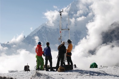
We assess the performance of incoming longwave radiation models in the Himalaya, using data from eight automatic weather stations. In the Himalaya, clouds often form locally, and we show that a new model, which uses relative humidity as a parameter, performs better than the ones available in previous literature. Source: Usmar Helleman.

1. INTRODUCTION

Meltwater from snow and ice forms an important part of the hydrological cycle in the upper reaches of many of Asia's large rivers (Lutz et al., 2014). The energy balance over glacier and snow surfaces, which determines the melt, is generally dominated by the shortwave and longwave radiative fluxes (e.g., Azam et al., 2014). During daytime, the net shortwave radiation is the major energy flux term, whereas in cloudy conditions above fresh snow, as well as during the night, net longwave radiation becomes the most important driver for melt (Müller, 1985; Granger and Gray, 1990; Bintanja and van den Broeke, 1996; Litt et al., 2019). Clouds do not only decrease the shortwave radiation that reaches the surface but they also have the potential to emit more longwave radiation towards the surface (LW_in) than the gaseous atmosphere due to their larger optical thickness, giving them a higher effective emissivity.

Measurements of longwave radiation in mountainous regions are relatively rare, with a large focus on the Alps (e.g., Marty et al., 2002). With a lack of measurements, surface energy balance studies generally use empirical models to determine LW_in. A number of parameterizations exist that describe LW_in using air temperature, water vapour pressure and a cloud factor derived from the atmospheric transmissivity (Marthews et al., 2012; Juszak and Pellicciotti, 2013; Formetta et al., 2016). These models were not developed or tested in humid high‐mountain environments, typical for the tropical Andes or the Himalaya. The high elevations give rise to low pressures and temperatures, resulting in relatively low vapour pressures. For the gaseous atmosphere, this means that other radiators, such as CO₂, could contribute relatively more to the LW_in (Philipona et al., 2004). Furthermore, during the wet season, abundant clouds are formed locally in the mountains. Hence, the clouds in this environment often resemble a ground fog, as seen from the surface, instead of passing at a higher altitude with corresponding lower temperatures. This could lead to an underestimation of LW_in in cloudy conditions. Simple parameterizations that include cloud cover also have difficulties in adequately accounting for longwave radiation during the early morning, evening and night, where cloud cover is generally unknown if retrieved through shortwave radiation measurements. Sicart et al., 2010 show that for the tropical Andes the variability of LW_in is predominately driven by cloud cover rather than air temperature or the emitting low atmosphere.

Here, we analyse new multi‐annual time series of climatic data in three Himalayan catchments, which enable us to (a) investigate the importance of longwave radiation in the total net radiative budget of high‐altitude catchments in the Himalaya (see also Litt et al., 2019), (b) test standard approaches to model longwave radiation and (c) develop a new longwave parameterization suitable for high altitude conditions. This paper is divided into three parts: we first present the available data and discuss the radiative budget. Second, we discuss existing longwave parameterizations and test their performance for our Himalayan stations. Finally, we propose a new longwave parameterization that is easy to implement using inexpensive measurements.

2. OBSERVATIONS OF LW_IN IN THE HIMALAYA

2.1. Stations

Meteorological data used in this study has been collected at eight different automatic weather stations (AWSs, see Table 1, Figure 1), three of which are located in the Langtang catchment (Kyanjing, Yala Base camp and Yala Glacier), and three in the Khumbu catchment (Naulek, Mera and Changri Nup), both in Nepal. These two catchments have a monsoon‐dominated climate in summer. Two additional stations are located on the Chhota Shigri Glacier, where summers are dryer (Azam et al., 2014). Figure 2 illustrates the difference in annual cycle between Yala Basecamp, which is monsoon‐dominated, and Chhota Shigri Moraine, which is dryer in summer and wetter in winter. To differentiate between the different seasons in the monsoon‐dominated Himalaya, we separate our data into a wet monsoon season (June–September) and a dry season (October–May), based on precipitation measurements (e.g., Immerzeel et al., 2014). The Chhota Shigri stations do not have precipitation measurements for direct comparison, but we refer to Azam et al. (2014) for more details on the annual cycle of precipitation in that area.

Table 1.

Hourly AWS data used in this study

AWS	Latitude [deg]	Longitude [deg]	Elevation [m.a.s.l.]	Period	Data pointsa	Sensor model, error and initial height
Kyanjing	28.211	85.569	3,862	10/2015–11/2018	20,454 (95%)	Rotronic HC2S3 ± 0.1°C, ± 0.8% RH, 1.9 m Kipp & Zonen CNR4 ± 3%, 2.3 m
Yala basecamp	28.232	85.610	5,090	10/2015–10/2018	26,294 (61%)	Rotronic HC2S3 ± 0.1°C, ± 0.8% RH, 1.8 m Kipp & Zonen CNR4 ± 3%, 2.4 m
Yala glacier	28.235	85.618	5,350	05/2016–04/2018	17,249 (92%)	Rotronic HC2S3 ± 0.1°C, ± 0.8% RH, 2.2 m Kipp & Zonen CNR4 ± 3%, 2.5 m
Naulek	27.718	86.897	5,354	11/2012–11/2016	59,925 (83%)	Vaisala HMP155 ± 0.2°C, ±2% RH, 1.4 m Kipp & Zonen CNR4 ± 3%, 0.7 m
Mera	27.707	86.874	6,352	11/2013–08/2016	42,252 (83%)	Vaisala HMP155 ± 0.2°C, ±2% RH, 1.7 m Kipp & Zonen CNR4 ± 3%, 1.3 m
Changri Nup	27.983	86.779	5,360	11/2014–11/2017	53,061 (88%)	Vaisala HMP45C ±0.3°C, ±2% RH, 1.6 m Kipp & Zonen CNR4 ± 3%, 1.1 m
Chhota Shigri glacier	32.241	77.518	4,670	08/2012–10/2013	6,311 (81%)	Campbell155A ±0.1°C, ±1% RH, 2.5 m Kipp & Zonen CNR4 ± 3%, 1.8 m
Chhota Shigri moraine	32.230	77.506	4,683	08/2009–09/2013	20,877 (91%)	Campbell H3‐S3 XT ±0.1°C, ±1.5% RH, 1.5 m Kipp & Zonen CNR1 ± 10%, 2.5 m

^aDatapoints are the number of accurate hourly measurements of LW_in and the percentage where LW_in, RH, T_air and SW_in are available at the same time.

Figure 1.

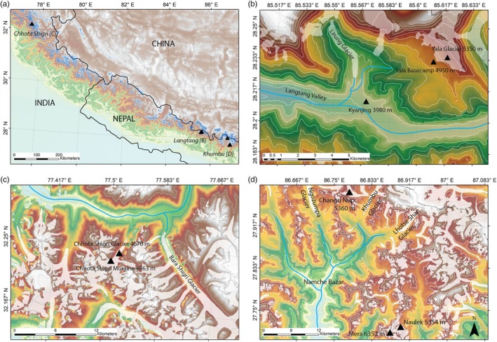
Locations of our study sites in the Himalaya (a), with detailed maps of Langtang Valley (b), Chhota Shigri (c) and Khumbu Valley (d), including names of main glaciers and settlements. The measurement sites are indicated with black triangles

Figure 2.

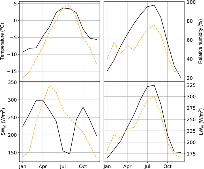
Monthly means of temperature (a), relative humidity (b), incoming shortwave radiation (c) and incoming longwave radiation (d) from hourly data at Yala basecamp between 2016 and 2018 (solid lines) and hourly data at Chhota Shigri moraine between 2009 and 2013 (dashed lines)

2.2. Atmospheric conditions

We used the Yala Basecamp (Yala BC) station as a reference, and to calibrate model parameters. We chose this station, since it has the most consistent data record, and is intermediate in elevation (5,090 m.a.s.l.). The mean meteorological conditions for Yala BC are summarized in Figures 2 and 3. During the dry season, relative humidity increases from sunrise to sunset, after which it drops again, coinciding with the wind direction reversing from up‐valley to down‐valley (not shown). During the monsoon, the air is practically saturated at night, with a slight average drop in relative humidity during the day, when temperatures increase rapidly. LW_in has a diurnal cycle in the dry season that better resembles the relative humidity curve than the temperature curve. In monsoon, the LW_in seems to follow more closely the temperature variations, although the LW_in peak is later than the actual temperature peak (see Figures 3a,d).

Figure 3.

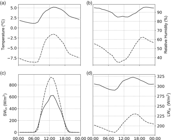
Mean diurnal cycles of air temperature (a), relative humidity (b), SW_in (c) and LW_in (d) measured at Yala BC in the wet season (monsoon, solid lines) and dry season (dashed lines) between 2015 and 2018

Mean hourly LW_in at Yala BC during the dry season is 206 W/m². In monsoon, the mean hourly flux is 306 W/m², with a smaller diurnal variability than the dry season. Patterns are similar at all other locations, with mean fluxes ranging from 166 W/m² near the summit of Mera to 245 W/m² at the lowest station in Kyanjing during the dry season and 271 and 335 W/m² in the monsoon respectively.

While incoming shortwave radiation is generally considered the most important flux for ice or snow melt, longwave radiation plays a considerable role as well (Sicart et al., 2005; Azam et al., 2014; Huintjes et al., 2015a; Huintjes et al., 2015b). During monsoon, the LW_in at Yala BC amounts to 36% of the total incoming radiation during daytime (ranging between 27 and 57% when all monsoon‐dominated stations are considered), compared with 21% during the dry season (ranging between 20 and 30% when all monsoon‐dominated stations are considered). These values are considerably larger when the mean over the entire day is taken (61 and 44% for Yala BC for wet and dry seasons, respectively).

3. EXISTING LW_IN PARAMETERIZATIONS

3.1. Parameterization description

The LW_in generally includes two components: one from the gaseous atmosphere (water vapour and other gases), and one from clouds, which mostly consists of water droplets or icy particles. In steep mountainous terrain, nearby high surfaces can cause an additional contribution close to the horizon. We assume this component to be relatively small in the following, given the generally small solid angle and high incidence angle of the radiation. The most common way to represent LW_in under both clear and cloudy conditions is by using a version of the Stefan‐Boltzmann law:

$${\mathrm{LW}}_{\text{in}}={\epsilon }_{\mathrm{eff}}\sigma T^4,$$ (1)

where ε_eff is the effective emissivity of the atmosphere, in theory ranging from 0 to 1, σ is the Stefan Boltzmann constant (5.67 x 10⁻⁸ W m⁻² K⁻⁴) and T is the air temperature at screen level (K). In the absence of clouds, the effective emissivity can be represented by a clear‐sky emissivity ε_clear. A standard approach to compute clear‐sky emissivity, used in various climates, was proposed by (Brutsaert, 1975):

$${\epsilon }_{\text{clear}}=C{\left(e/T\right)}^{\frac{1}{m}},$$ (2)

where e is the atmospheric vapour pressure (hPa), m = 7, and C represents the relation between vapour pressure and temperature near the ground, which can be adapted to the local climate. While Brutsaert (1975) gives C = 1.24, Sicart et al., 2010 find C = 1.15 for a mountainous tropical climate, while Konzelmann et al. (1994) finds m to be larger than 7 but C to be only 0.443 on the Greenland ice‐sheet.

Another approach was proposed by Dilley and O'Brien (1998) and found to provide best results in a comparison study of longwave parameterizations applicable to melting glaciers in the Alps (Juszak and Pellicciotti, 2013), as well as multiple sites in China and North as well as South America (Flerchinger et al., 2009; Marthews et al., 2012). The equation derived in those studies to estimate clear sky emissivity is:

$${\epsilon }_{\text{clear}}=\frac{59.38+113.7{\left(\frac{T}{273.16}\right)}^6+96.96\sqrt{\frac{4.65e}{25T}}}{\sigma T^4}.$$ (3)

In Section 3.2, we compare these two models to our data and test their suitability for the high‐altitude environments in the Himalaya.

A number of empirical approaches to model the effective emissivity for overcast conditions also exist (see Juszak and Pellicciotti, 2013 and references therein for an overview). Juszak and Pellicciotti (2013) find the parameterization proposed by Unsworth and Monteith (1975) for cloudy conditions, in combination with the relation of Dilley and O'Brien (1998) for clear sky emissivity, to be performing the best for data in the Swiss Alps (henceforth referred to as the UM model). The UM model is dependent on the atmospheric transmissivity τ_atm, which is derived from the measured daytime surface incoming shortwave radiation SW_in and the theoretical potential clear‐sky incoming shortwave radiation SW_pot:

$${\tau }_{\mathrm{atm}}={\mathrm{SW}}_{\text{in}}/{\mathrm{SW}}_{\mathrm{pot}}.$$ (4)

The effective emissivity is then found as follows:

$${\epsilon }_{\mathrm{eff}}=\left(1+a\bullet (1-{\tau }_{\mathrm{atm}}\right))\bullet {\epsilon }_{\text{clear}}+b\bullet \left(1-{\tau }_{\mathrm{atm}}\right),$$ (5)

where a and b are location‐specific parameters and equal to a = −0.84 and b = 0.84 in the original model proposition.

Sicart et al., 2010 present another approach of parameterising LW_in, based on measurements in the tropical Andes. They find two peaks in the occurrence distribution of the atmospheric transmissivity, coinciding with very cloudy and clear conditions, and introduce a cloud factor F to describe the effective emissivity, such that ε_eff = F ∙ ε_clear. They suggest that beyond a transmissivity of 0.8 the cloud factor reaches unity, resulting in:

$$F=\left\{\begin{array}{c}\begin{array}{cc}1.67-{\tau }_{\mathrm{atm}}0.83& {\tau }_{\mathrm{atm}}\le 0.8\\ 1& {\tau }_{\mathrm{atm}}>0.8\end{array}\\ \end{array}\right.$$ (6)

This model was found to perform well in the tropical Andes, and we refer to this model as the S model.

To distinguish between clear‐sky and cloudy conditions, an accurate SW_pot has to be computed, which depends on local topographic shading as well as the clear sky transmissivity. We first determine SW_{pot_clear} at hourly time steps between 6:00 a.m. and 7:00 p.m. local time using the algorithm employed by ArcGis, assuming a transmissivity of 1 (Fu and Rich, 2002). We use the NSIDC 8‐m HMA DEM (Shean, 2017) to account for accurate shading. Choosing all measurements of SW_in larger than 1,000 W/m², which we assume to be definitely cloud‐free measurements. We determine the atmospheric transmissivity with respect to the calculated SW_{pot_clear} under these conditions as ${\tau }_{\text{clear}}=\frac{{\mathrm{SW}}_{\text{in}}}{{\mathrm{SW}}_{\mathrm{pot}\text{\_}\text{clear}}}$. Clear‐sky transmissivity varies between the sites, with lowest values at the lowest site, Kyanjing (0.72), and highest on the highest site, Mera (0.76), corresponding to a decrease in atmospheric pressure or decreasing atmospheric thickness. We then use the average value 0.746, which is nearly identical to the commonly used 0.75 from Hock (1999) to calculate the actual potential incoming shortwave radiation SW_{pot as follows}:

$${\mathrm{SW}}_{\mathrm{pot}}={\mathrm{SW}}_{\mathrm{pot}\_\text{clear}}\cdot {\tau }_{\text{clear}},$$ (7)

At night, the transmissivity τ_atm was linearly interpolated between the last daytime point and the first daytime point the next day.

Table 2 summarizes the different models we test in this paper.

Table 2.

Summary of existing LW_in models

Model	Reference	Relation	Required input
S (clear)	Brutsaert (1975) Sicart et al. (Sicart et al., 2010)	${\epsilon }_{\text{clear}}=C{\left(e/T\right)}^{\frac{1}{m}}$	Temperature (measured) Relative humidity (measured) Clear‐sky threshold (e.g., from SWin)
D + O (clear)	Dilley and O'Brien (1998)	${\epsilon }_{\text{clear}}=\frac{59.38+113.7{\left(\frac{T}{273.16}\right)}^6+96.96\sqrt{\frac{4.65e}{25T}}}{\sigma T^4}$	Temperature (measured)relative humidity (measured) Clear‐sky threshold (e.g., from SWin)
UM (clear + cloudy)	Unsworth and Monteith (1975) Juszak and Pellicciotti (2013)	εeff = (1 + a ∙ (1 − τatm )) ∙ εclear + b ∙ (1 − τatm)	Temperature (measured) Relative humidity (measured) SWin (measured) SWpot (high‐resolution DEM [measured], Clear‐sky transmissivity [measured and/or assumed]) Night time transmissivity (assumed)
S (clear + cloudy)	Sicart et al., 2010	εeff = F ∙ εclear $F=\left\{\begin{array}{c}\begin{array}{cc}1.67-{\tau }_{\mathrm{atm}}0.83& {\tau }_{\mathrm{atm}}\le 0.8\\ 1& {\tau }_{\mathrm{atm}}>0.8\end{array}\\ \end{array}\right.$	Temperature (measured) Relative humidity (measured) SWin (measured) SWpot (high‐resolution DEM [measured], Clear‐sky transmissivity [measured and/or assumed]) Night time transmissivity (assumed)

3.2. Performance in the Himalaya

We tested the performance of the LW_in parameterizations that performed well in the Alps and the tropical Andes using our measured LW_in in the Himalaya. We first assess the two selected clear‐sky parameterizations before assessing the entire time series.

Figure 4 shows the clear‐sky description of LW_in by Brutsaert (1975) and Sicart et al., 2010, compared with measurements with a transmissivity larger than 0.9 at the three Langtang sites. Figure 4 indicates that there are data points with high emissivities included for deduced transmissivities larger than 0.9. This scatter of high emissivity data points is more prominent at higher elevation. These data points probably indicate partial cloud cover, while still having high incoming shortwave radiation conditions (see our detailed discussion in Section 5). Sicart et al., 2010 note a similar change in their C parameter with altitude, which they attribute to changing temperature and humidity profiles. Our observations also show that the originally proposed parameter of C = 1.24 provides a somewhat better description to LW_in than the value of C = 1.15, as determined by Sicart et al., 2010 for hourly data in the Andes. Nevertheless, both descriptions generally underestimate the clear‐sky LW_in for our stations in the Himalaya, indicating that a higher value of C is needed. The model by Dilley and O'Brien (1998) generally has a lower bias, as indicated in Figure 5, but also does not capture the data points with high LW_in. Furthermore, it overestimates LW_in at the very lowest values.

Figure 4.

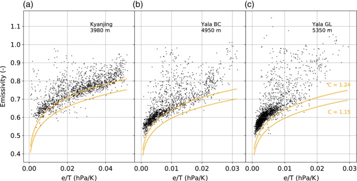
Measured clear‐sky emissivity at Kyanjing (a), Yala BC (b) and Yala GL (c) for daytime cases where τ _atm > 0.9 (black dots), compared to the models (solid lines) of Brutsaert (1975) with the original (C = 1.24) and an adapted parameter C (1.15, Sicart et al., 2014)

Figure 5.

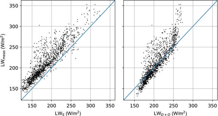
Measured (LW_meas) versus modelled LW_in for the Sicart et al. (2010) (LW_s) and Dilley and O'Brien (1998) (LW_D + O) parameterization for daytime clear‐sky conditions (τ_atm > 0.9) for hourly data of Yala BC between 2015 and 2018

For the full time series, including cloud cover, we assess the S and UM parameterizations, as described above. Figure 6 compares the hourly LW_in measurements at Yala BC to these two parameterizations. The UM model with the parameters as in the literature, greatly overestimates LW_in at low values, and underestimates LW_in at high values. The S model reproduces the variability at low LW_in values well, but has a negative bias stemming from the choice of C parameter for the clear‐sky conditions, as shown in Figures 4 and 5. For the high and intermediate LW_in values there is a general negative bias, except for the very highest values of LW_in.

Figure 6.

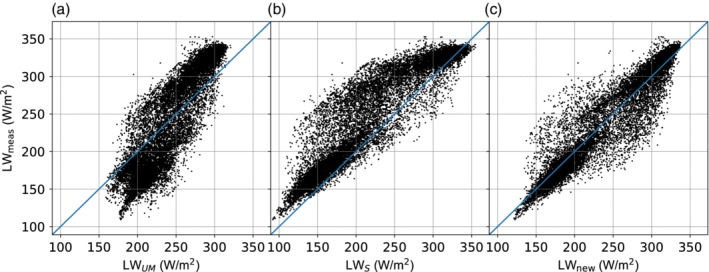
Measured versus modelled LW_in for the UM model (a), the S model (b) and the new parameterization described in Section 4 (c) for hourly data of Yala BC between 2015 and 2018

4. A NEW INCOMING LONGWAVE PARAMETERIZATION

4.1. Rationale

The previous section indicates relatively poor performance of existing longwave parameterizations in the Himalaya. It shows that the transmissivity is not necessarily a good measure of cloudiness, and that LW_in is generally underestimated under cloudy conditions. This indicates a need for a separate calibration for high‐mountain environments in the Himalaya, or a new LW_in parameterization. The similarity in shape of the diurnal cycles of LW_in and relative humidity, with the shape of the LW_in curve being in between the air temperature and relative humidity curves (see Figure 3), motivated us to consider relative humidity as a possible variable for describing LW_in in the Himalaya, next to air temperature. Figure 7 shows the effective emissivity as a function of relative humidity, vapour pressure and transmissivity. From the figure, it is clear that many of the data points cluster into two branches: a clear‐sky branch with low emissivity, and a branch with emissivities close to unity. The latter condition is consistent with optically thick clouds at the temperature close to that of the sensor, indicating local and low cloud formation, like the thick cumulus cloud typically observed at the sites. In between the two branches, there is a scatter of data points, consistent with broken clouds and/or clouds at higher altitudes. These intermediate points show only a slight correlation with shortwave transmissivity, with a large scatter and many data points having very high transmissivities (see Figure 7c). Also note that at high emissivities, there is almost no dependence of LW_in on the transmissivity, in contrast to what the UM and S models assume.

Figure 7.

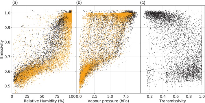
Effective emissivity as a function of relative humidity (a), vapour pressure (b) and transmissivity (c) or hourly data of Yala BC between 2015 and 2018. Dark points indicate daytime, whereas lighter points indicate night time

Figure 7 also shows that relative humidity is generally good at separating out the two branches. Especially at night, when there are no transmissivity measurements possible, thick local clouds form only at very high relative humidity. We chose a simple parameterization using only temperature and relative humidity, which can represent both the clear‐sky and the cloudy branch:

$${\mathrm{LW}}_{\text{in}}=c_1+c_2\mathrm{RH}+c_3\sigma T^4$$ (8)

We tried multiple relations that included temperature and relative humidity, but the best ones gave similar results as the above simple relationship. Based on Figure 7a, we separate the data into two branches using only relative humidity as a criterion: at night (incoming shortwave radiation is less than a relatively small threshold, which we took as 50 W/m² in our case, with smaller values not significantly affecting the results) the cloudy branch is described by a relative humidity larger than 80%, whereas during the day this threshold was set to 60%. A wide range of threshold values were tested, but values of the daytime relative humidity threshold between 40 and 80%, and night time values between 75 and 100%, gave root‐mean‐squared errors that differed less than 1 W/m² for Yala BC. The parameters obtained from fitting Equation 8 for the two different branches for Yala BC are shown in Table 3.

Table 3.

Parameters for the new model described in Equation 8

	c1	c2	c3
Clear branch (RHday < 60%; RHnight < 80%)	−75.28	0.82	0.79
Cloudy branch (RHday ≥ 60%; RHnight ≥ 80%)	−212.59	1.89	1.06

4.2. Performance of the new parameterization

The performance of the new parameterized hourly LW_in, compared with the measured values at Yala BC, is shown in Figure 6c. There is generally a very good agreement between the two, with the largest deviations caused by the data points representing intermediate cloud conditions. A comparison of the different panels in Figure 6 shows that the new parameterization performs better than the two other parameterizations with the parameters from the literature, with notably less deviation during periods with high LW_in, which are mostly encountered during the wet season.

The mean diurnal cycle of LW_in is also reasonably represented by the new parameterization and shows good agreement with measurements, especially at night (see Figure 8, Table 4). During the day, the diurnal cycle of the new model peaks too late, and is more weighed towards the relative humidity curve. On the other hand, the S model has a diurnal cycle that follows the temperature cycle too much, with a peak that is too early. The S model consistently shows the large negative bias that is also clear from Figure 6. The UM model shows much more variability in daytime LW_in and has a negative bias in the wet season, whereas it has a positive bias at night in the dry season.

Figure 8.

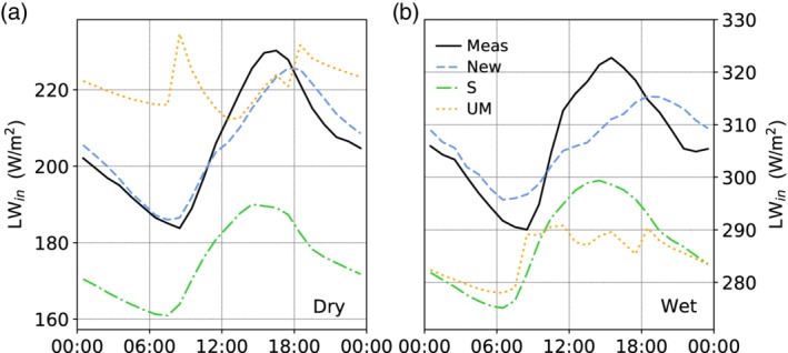
Mean diurnal cycles of measured LW_in (solid lines), and for the UM model (dotted line), the S model (dashed line) and the new parameterization (dashed line) for the dry season (a) and the wet season (b) at Yala BC between 2015 and 2018. Note that the LW_in range for is different for both seasons

Table 4.

Statistical fit of all three methods (UM model, S model and the model from this study), on hourly data from all eight stations, described by the Nash‐Sutcliffe efficiency (NSE), the mean bias error (MBE) and the root mean square error (RMSE), with bold numbers indicating the best model

UM/S/this study	NSE [−]	MBE [W m−2]	RMSE [W m−2]
Kyanjing	0.76/0.49/0.77	2/27/−4	28/41/27
YalaBC	0.70/0.67/0.90	−2/27/0	36/38/21
YalaGL	0.74/0.63/0.91	2/32/0	34/41/20
Naulek	0.66/0.36/0.87	11/44/10	37/50/23
Mera	0.65/0.23/0.81	0/48/8	39/58/28
Changri Nup	0.72/0.51/0.82	3/38/11	33/44/27
Chhota Shigri GL	0.69/0.54/0.68	−5/27/9	31/38/31
Chhota Shigri M	0.50/0.39/0.58	−4/33/23	44/49/40

Table 4 compares the performance of the three assessed parameterizations for all eight stations in the Himalaya, showing very similar relative results for all stations. The UM and S models perform the worst at the high‐altitude sites in Khumbu, whereas for the new parameterization the performance is less impacted there. All three models have a relatively poor performance for the Chhota Shigri Moraine site, which shows relatively more intermediate LW_in cases at relative humidities smaller than 60% than the other sites. It also has more intermediate transmissivity cases. For the Chhota Shigri sites, the existing models perform relatively better compared to the new model from this study.

4.3. Impact of the calibration site

We have now compared our new parameterization, calibrated at Yala Basecamp, to the S and UM models, calibrated using data from the Andes and Alps. Hence, it is possible that a calibration site in the Himalaya will change the S and UM models and will improve performance in the Himalaya. We tested the ability of all three models to reproduce the measured LW_in by fitting the model to the measurements for all stations separately using linear least‐squares. The fitted parameters for Yala Basecamp for the S and UM models are given in Table 5.

Table 5.

Model parameters for Yala basecamp for the S and UM models

Model	Parameters
UM	a = 2.50; b = −1.56
S	C = 1.13; m = 9.09

The performance metrics from this exercise are summarized in Table 6. It is clear that the S and UM models indeed show much better performance of all errors when fitted to the data at the site itself, compared with the literature values of the parameters. They are now more comparable to the new method presented in this work. In contrast, the new model shows only a slight improvement in root mean square error (RMSE), indicating that the parameterization from Yala Basecamp is already close to ideal for many of the stations. The main improvement for the new model is in the mean bias error. The new method still outperforms the S and UM models for all stations except at Chhota Shigri Moraine, where all methods show the worst performance. Figure 9 indicates that the new parameterization performs especially well at high LW_in values, which are the most relevant for glacier melt calculations. Furthermore, the UM model gives slightly more scatter in the residuals for low LW_in values than the other two models.

Table 6.

Statistical fit of all three methods (UM model, S model and the model from this study), locally fitted, on hourly data from all eight stations, described by the Nash‐Sutcliffe efficiency (NSE), the mean bias error (MBE) and the root mean square error (RMSE), with bold numbers indicating the best model

UM/S/this study	NSE [−]	MBE [W m−2]	RMSE [W m−2]
Kyanjing	0.83/0.67/0.84	1/−2/0	24/32/23
YalaBC	0.86/0.81/0.90	1/−2/0	25/28/21
YalaGL	0.88/0.84/0.92	1/−2/‐2	24/27/19
Naulek	0.82/0.84/0.89	6/−1/0	27/26/21
Mera	0.81/0.82/0.86	2/−1/−4	29/28/25
Changri Nup	0.86/0.84/0.87	4/−1/0	24/25/23
Chhota Shigri GL	0.79/0.77/0.77	1/−1/0	26/27/27
Chhota Shigri M	0.67/0.67/0.74	5/−1/0	35/36/32

Figure 9.

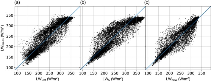
Measured versus modelled LW_in for the UM model (a), the S model (b) and the new parameterization described in Section 4 (c), with locally fitted parameters, for hourly data of Yala BC between 2015 and 2018

4.4. Implications for glacier melt calculations

LW_in is an important component contributing to the glacier melt in the Himalaya (Litt et al., 2019). We calculated melt on our on‐glacier site on Yala Glacier (2016 and 2017) using the different parameterizations, as available in the literature, for LW_in and compared the results against the full energy balance using only measured fluxes (Figure 10). For details on the energy balance please refer to Litt et al. (2019). Using the S model results in an underestimation of melt of 0.33 m w.e. (30%) in 2016 and 0.18 cm in 2017 (18%), which had a shortened measurement period. The new parameterization decreases this offset to 0.12 m w.e. (12%) and 0.06 m w.e. (6%), respectively. As is obvious from the diurnal cycle (Figure 10), the new model especially improves the large offset due to the biases in LW_in. In addition, the original S and UM models overestimate the refreezing considerably due to underestimated LW_in. When the locally optimized S and UM models are used, the UM model gives almost identical results to the blue line in Figure 10. The optimized S model overestimates the melt fluxes at night. In 2016, it underestimates the daytime flux, giving an overall match of the cumulative melt within 0.01 m w.e. In 2017, the optimized S model also slightly overestimates the daytime flux, giving a total overestimation of 0.06 m. w.e. While a number of uncertainties exist in the total surface energy balance, most notably related to the roughness of the ice or snow surface influencing the turbulent fluxes (Litt et al., 2019), these results show that the differences in the LW_in parameterization can also greatly influence melt calculations, especially during the wet monsoon.

Figure 10.

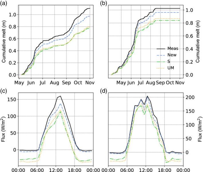
Cumulative melt at Yala glacier calculated from the full energy balance in 2016 (a) and 2017 (b), as well as the corresponding mean diurnal cycle (c, d). Lines indicate measurements (solid lines), and melt or fluxes obtained from the UM model (dotted line), from the S model (dashed line), and with the new parameterization (dashed line)

5. CONCLUSIONS AND DISCUSSION

We have investigated the applicability of existing parameterizations for LW_in in the Himalaya, based on near‐surface air temperature, vapour pressure and shortwave transmissivity, and found that they have relatively large biases. Generally, they underestimate LW_in, especially in wet and cloudy (monsoon) conditions. We propose a new empirical LW_in parameterization for the Himalaya, based only on near surface air‐temperature and relative humidity. The new parameterization performs well for all eight analysed stations in the Himalaya, with NSE above 0.7 and RMSE below 30 W/m² for six stations, even with a fixed parameterization. We obtain especially good performance in wet and cloudy conditions, such as those encountered during the monsoon. Furthermore, it has the benefit to work well at night, when no transmissivity information is available. Simple thresholds, such as the time of sunset and sunrise, can be used to separate night and day. Another advantage of our proposed method is that near surface air‐temperature and relative humidity are easy to measure, requiring only small and relatively inexpensive equipment. This is greatly beneficial for future work in the Himalaya, where measurements of radiation are very sparse, and equipment is difficult to install and maintain. The longwave contribution can be over half of the incoming radiation in the monsoon season and we show that the choice of parameterization greatly affects glacier melt models for the presented catchments in the Himalaya. Hence, a good representation of LW_in is essential for detailed glacier energy balance models, and hydrological modelling of catchments with snow and ice. Although our stations were separated over many hundreds of kilometres, the performance of the new parameterization will need to be verified for other mountainous environments.

One of the reasons why the simple parameterization works especially well in the presented monsoon‐dominated catchments is that most data points indicate either clear‐sky or cloud‐covered conditions, with relatively infrequent intermediate cases. At Yala Basecamp the intermediate cases represent roughly 25% of the data points. This is consistent with the idea that many clouds form against the mountain slopes themselves, instead of drifting over at higher altitudes. In this study, we did not fit the intermediate cloud points separately from the clear‐sky and cloudy branches, since we found it difficult to select these intermediate cloud cases based on measurements of parameters other than LW_in. This causes our fit to deviate slightly from the dense cloudy branch, as seen in Figure 6c. More complex parameterizations could take the intermediate cases into account separately to increase performance even further, if the intermediate cases can be separated somehow. We do note that these intermediate cases occur almost exclusively at low wind conditions, with wind speeds less than 2 m/s.

All models had the worst performance at the Chhota Shigri Moraine site, which shows a relatively large occurrence of intermediate emissivities at low relative humidity, and intermediate transmissivities at low emissivites. In contrast, the Chhota Shigri Glacier site has more intermediate emissivities at high relative humidity. In both cases, it is possible that the relative humidity that is measured at 2 m above the surface does not represent the atmosphere above it very well. In warm and dry conditions, where the glacier is melting, the relative humidity directly above the glacier is probably significantly higher than the atmosphere tens of meters above it. In the monsoon, the relative humidity will be high in the entire atmosphere, and there will probably be less of a gradient in that period for the monsoon‐dominated sites. Above rock, radiative heating could cause strong temperature and relative humidity gradients. Exploratory experiments in Langtang valley, where we took measurements with a temperature and relative humidity sensor (iMet‐QX, ±0.3°C, ±5%) on a small drone, show such gradients exist up to at least 10 m above the surface (see Figure 11). Improvements in the performance of the parameterizations in cases of nonlocal clouds might thus be achieved by setting up sensors at slightly higher heights above the surface, or having two sets of sensors at two different heights, a few metres apart, to correct for steep gradients. However, the first suggestion is probably impractical in the Himalaya. In any case, more research and measurements are needed to quantify boundary layer effects in the Himalaya.

Figure 11.

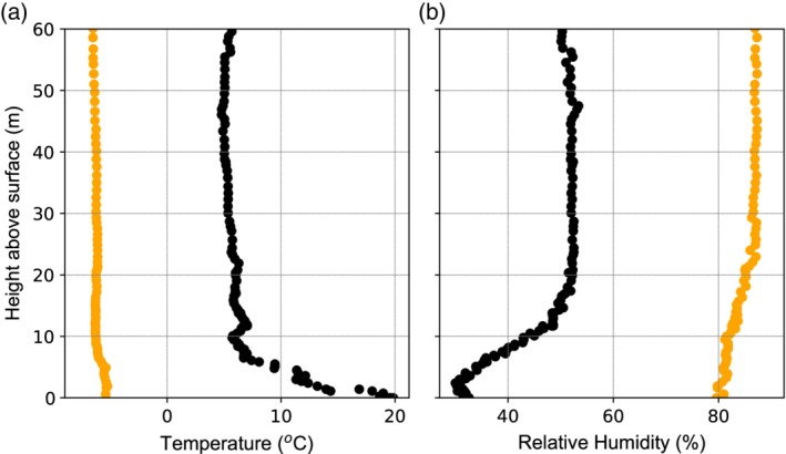
Vertical profiles of temperature (a) and relative humidity (b) taken above a rocky site on April 19, 2018 at 12:30 (dark), and during snowfall on April 25, 2018 at 17:00 (light)

During the day, the cloudiness derived from the longwave radiation does not seem to correspond well to the transmissivity, as derived from the incoming shortwave radiation (see Figure 7c). An explanation for this could be that the shortwave radiation is mainly dominated by direct sunlight from the direction of the sun, whereas the sources of longwave radiation are more uniformly distributed across the sky. Furthermore, the theoretically calculated potential clear‐sky shortwave radiation is sometimes lower than the measured SW_in. Reflection from nearby (snowy) surfaces and small clouds, as well as enhanced radiation due to a thin cloud layer, could further influence the shortwave measurements to limit the effectiveness of transmissivity calculations in mountainous regions. In the dry season, clear‐sky SW_in could be determined empirically, but in the wet season clear‐sky conditions are not frequent enough for such an approach. All‐sky imaging (e.g., Pfister et al., 2003) might improve the estimation of cloud cover for LW_in modelling if high accuracy is required. Furthermore, images could help identify the differences between thick cumulus and thin cirrus conditions, in order to understand the performance of the model. Remotely sensed cloud products, such as those from images, radar, or laser altimetry could further help to understand the cloud properties. However, due to the generally limited repeat time and spatial resolution, they will be most useful for calibration purposes and qualitative comparisons. However, the relative humidity will probably be a necessary parameter in the cloudy wet season, since relative humidity could act as a measure of the altitude of the cloud above the station, and hence the temperature difference with respect to the temperature measured at the station.

Although the above results focus on the Himalaya, the new parameterization could potentially be used in other mountainous regions as well. The eight stations used in this study already reflect some differences in climatic setting, but we test the parameterization on three very different locations to further illustrate its potential outside the Himalaya. We use publicly available hourly data from an AWS on Hintereisferner, located in the Austrian Alps (46.80^oN, 10.76°E) at 3026 m.a.s.l., between October 7, 2010 and October 11, 2012 (Stocker‐Waldhuber et al., 2013a, 2013b, 2013c), as well as half‐hourly data on Saint‐Sorlin glacier in the French alps at 2700 m.a.s.l. between January 1, 2010 and December 31, 2011 (45.17^oN, 6.17°E), and Zongo glacier in the Bolivian Andes at 5050 m.a.s.l. between August 5, 2004 and December 14, 2005 (16.25^oS, 68.17^oW). The agreement of the new parameterization, using the parameters given in Table 3, with the measurements of LW_in is shown in Figure 12. The performance is comparable to that for Yala BC for Hintereisferner. For Saint‐Sorlin, the scatter is larger, partly from more intermediate cloud conditions. Furthermore, there is a group of night time points that have high emissivity, but relative humidity lower than 80%. Nevertheless, performance of the new parameterization for Saint‐Sorlin is comparable to Changri Nup. Zongo data show only very few intermediate cloud cases, but shows offsets that are compatible with what is shown by Sicart et al., 2010 and Figure 4. With the Yala BC parameters, the new parameterization still performs better for Zongo than for Chhota Shigri Moraine, but a local calibration greatly improves the parameterization here, making it comparable in performance to Yala BC. These data from other mountain ranges suggest that future work in other mountainous regions could also greatly benefit from the parameterization presented here.

Figure 12.

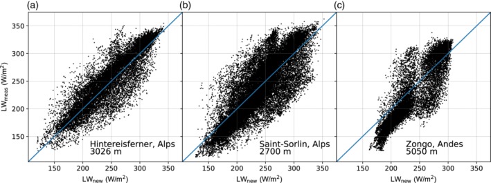
Measured versus modelled LW_in for Hintereisferner, Austria, between October 2010 and October 2012 (a), saint‐Sorlin, France, between January 1, 2010 and December 31, 2011 (b), and for Zongo, Bolivia, between August 5, 2004 and December 14, 2005 (c)

AUTHOR CONTRIBUTIONS

R.J.d.K. and J.F.S. initiated the study and wrote the initial draft of the manuscript; R.J.d.K. designed the new parameterization; J.F.S. calculated the performance of the old parameterizations and performed the glacier melt modelling; M.L., P.W., I.K., W.W.I., M.F.A. and J.F.S. installed and maintained the instruments; all authors contributed to the editing of the manuscript.

de Kok RJ, Steiner JF, Litt M, et al Measurements, models and drivers of incoming longwave radiation in the Himalaya. Int J Climatol. 2020;40:942–956. 10.1002/joc.6249

REFERENCES

- Azam, M.F. , Wagnon, P. , Vincent, C. , Ramanathan, A.L. , Favier, V. , Mandal, A. and Pottakkal, J.G. (2014) Processes governing the mass balance of Chhota Shigri glacier (western Himalaya, India) assessed by point‐scale surface energy balance measurements. The Cryosphere, 8(6), 2195–2217. 10.5194/tc-8-2195-2014. [DOI] [Google Scholar]
- Bintanja, R. and van den Broeke, M.R. (1996) The influence of clouds on the radiation budget of ice and snow surfaces in Antarctica and Greenland ind summer. International Journal of Climatology, 16(11), 1281–1296. . [DOI] [Google Scholar]
- Brutsaert, W. (1975) On a derivable formula for long‐wave radiation from clear skies. Water Resources Research, 11(5), 742–744. [Google Scholar]
- Dilley, A.C. and O'Brien, D.M. (1998) Estimating downward clear sky long‐wave irradiance at the surface from screen temperature and precipitable water. Quarterly Journal of the Royal Meteorological Society, 124(549), 1391–1401. 10.1002/qj.49712454903. [DOI] [Google Scholar]
- Flerchinger, G.N. , Xaio, W. , Marks, D. , Sauer, T.J. and Yu, Q. (2009) Comparison of algorithms for incoming atmospheric long‐wave radiation. Water Resources Research, 45(3), W03423 10.1029/2008WR007394. [DOI] [Google Scholar]
- Formetta, G. , Bancheri, M. , David, O. and Rigon, R. (2016) Performance of site‐specific parameterizations of longwave radiation. Hydrology and Earth System Sciences, 20, 4641–4654. 10.5194/hess-20-4641-2016. [DOI] [Google Scholar]
- Fu, P. and Rich, P. M. (2002) ‘A geometric solar radiation model with applications in agriculture and forestry’, Computers and Electronics in Agriculture. Elsevier, 37(1–3), pp. 25–35. doi: 10.1016/S0168-1699(02)00115-1. [DOI] [Google Scholar]
- Granger, R.J. and Gray, D.M. (1990) A net radiation model for calculating daily snowmelt in open environments. Hydrology Research, 21(4–5), 217–234. 10.2166/nh.1990.0017. [DOI] [Google Scholar]
- Hock, R. (1999) A distributed temperature‐index ice‐ and snowmelt model including potential direct solar radiation. Journal of Glaciology, 45(149), 101–111. 10.1017/S0022143000003087. [DOI] [Google Scholar]
- Huintjes, E. , Neckel, N. , Hochschild, V. and Schneider, C. (2015b) Surface energy and mass balance at Purogangri ice cap, central Tibetan plateau, 2001–2011. Journal of Glaciology, 61(230), 1048 10.3189/2015JoG15J056. [DOI] [Google Scholar]
- Huintjes, E. , Sauter, T. , Schroter, B. , Maussion, F. , Yang, W. , Kropacek, J. , Buchroithner, M. , Scherer, D. , Kang, S. and Schneider, C. (2015a) Evaluation of a coupled snow and energy balance model for Zhadang glacier, Tibetan plateau, using glaciological measurements and time‐lapse photography. Arctic, Antarctic, and Alpine Research, 47(3), 573–590. 10.1657/AAAR0014-073. [DOI] [Google Scholar]
- Immerzeel, W.W. , Petersen, L. , Ragettli, S. and Pellicciotti, F. (2014) The importance of observed gradients of air temperature and precipitation for modeling runoff from a glacierized watershed in the Nepalese Himalayas. Water Resources Research, 50(3), 2212–2226. 10.1002/2013WR014506. [DOI] [Google Scholar]
- Juszak, I. and Pellicciotti, F. (2013) A comparison of parameterizations of incoming longwave radiation over melting glaciers: model robustness and seasonal variability. Journal of Geophysical Research: Atmospheres, 118(8), 3066–3084. 10.1002/jgrd.50277. [DOI] [Google Scholar]
- Konzelmann, T. , van de Wal, R.S.W. , Greuell, W. , Bintanja, R. , Henneken, E.A.C. and Abe‐Ouchi, A. (1994) Parameterization of global and longwave incoming radiation for the Greenland ice sheet. Global and Planetary Change, 9(1–2), 143–164. 10.1016/0921-8181(94)90013-2. [DOI] [Google Scholar]
- Litt, M. , Shea, J. , Wagnon, P. , Steiner, J. , Koch, I. , Stigter, E. and Immerzeel, W. (2019) Glacier ablation and temperature indexed melt models in the Nepalese Himalaya. Scientific Reports, 9(1), 5264 10.1038/s41598-019-41657-5. [DOI] [PMC free article] [PubMed] [Google Scholar]
- Lutz, A.F. , Immerzeel, W.W. , Shrestha, A.B. and Bierkens, M.F.P. (2014) Consistent increase in high Asia's runoff due to increasing glacier melt and precipitation. Nature Climate Change, 4(7), 587–592. 10.1038/nclimate2237. [DOI] [Google Scholar]
- Marthews, T.R. , Malhi, Y. and Iwata, H. (2012) Calculating downward longwave radiation under clear and cloudy conditions over a tropical lowland forest site: an evaluation of model schemes for hourly data. Theoretical and Applied Climatology, 107(3–4), 461–477. 10.1007/s00704-011-0486-9. [DOI] [Google Scholar]
- Marty, C. , Philipona, R. , Fröhlich, C. and Ohmura, A. (2002) Altitude dependence of surface radiation fluxes and cloud forcing in the alps: results from the alpine surface radiation budget network. Theoretical and Applied Climatology, 72(3–4), 137–155. 10.1007/s007040200019. [DOI] [Google Scholar]
- Müller, H. (1985) On the radiation budget in the alps. Journal of Climatology, 5(4), 445–462. 10.1002/joc.3370050411. [DOI] [Google Scholar]
- Pfister, G, McKenzie, R.L., Liley, J.B., Thomas, A., Forgan, B.W. and Long, C.N. (2003) Cloud coverage based on all‐sky imaging and its impact on the surface solar irradiance. Journal of Applied Meteorology, 42, 1421–1434. . [DOI] [Google Scholar]
- Philipona, R. , Dürr, B. , Marty, C. , Ohmura, A. and Wild, M. (2004) Radiative forcing‐measured at Earth's surface‐corroborate the increasing greenhouse effect. Geophysical Research Letters, 31, L03202 10.1029/2003GL018765. [DOI] [Google Scholar]
- Shean, D.E. (2017) High Mountain Asia 8‐meter DEMs Derived from Cross‐track Optical Imagery, Version 1 [Langtang subset]. Boulder, Colorado USA, Colorado USA: NASA National Snow and Ice Data Center Distributed Active Archive Center. 10.5067/0MCWJJH5ABYO. [DOI]
- Sicart, J.E. , Hock, R. , Ribstein, P. and Chazarin, J.P. (2010) Sky longwave radiation on tropical Andean glaciers: parameterization and sensitivity to atmospheric variables. Journal of Glaciology, 56(199), 854–860. 10.3189/002214310794457182. [DOI] [Google Scholar]
- Sicart, J.E. , Litt, M. , Helgason, W. , Tahar, V.B. and Chaperon, T. (2014) A study of the atmospheric surface layer and roughness lengths on the high‐altitude tropical Zongo glacier, Bolivia. Journal of Geophysical Research Atmospheres, 119, 3793–3808. 10.1002/2014JD021494. [DOI] [Google Scholar]
- Sicart, J.E. , Wagnon, P. and Ribstein, P. (2005) Atmospheric controls of the heat balance of Zongo glacier. Journal of Geophysical Research, 110, 1–17. 10.1029/2004JD005732. [DOI] [Google Scholar]
- Stocker‐Waldhuber, M. , Emprechtinger, M. , Fischer, A. (2013a) Continuous measurements of soil temperature at weather station HEF (Hintereisferner), Ötztal Alps, Austria, in 2010. Institute of Meteorology and Geophysics, University of Innsbruck, PANGAEA. 10.1594/PANGAEA.809096. [DOI]
- Stocker‐Waldhuber, M. , Emprechtinger, M. ; Fischer, A. (2013b) Continuous meteorological observations at weather station HEF (Hintereisferner), Ötztal Alps, Austria, in 2011. Institute of Meteorology and Geophysics, University of Innsbruck, PANGAEA. 10.1594/PANGAEA.809094. [DOI]
- Stocker‐Waldhuber, M. , Emprechtinger, M. , Fischer, A. (2013c) Continuous meteorological observations at weather station HEF (Hintereisferner), Ötztal Alps, Austria, in 2012. Institute of Meteorology and Geophysics, University of Innsbruck, PANGAEA. 10.1594/PANGAEA.809095. [DOI]
- Unsworth, M.H. and Monteith, J.L. (1975) Long‐wave radiation at the ground I. angular distribution of incoming radiation. Quarterly Journal of the Royal Meteorological Society, 101, 13–24. [Google Scholar]