Abstract
Accurate estimations of the vertical leaf nitrogen (N) distribution within a rice canopy is helpful for understanding the nutrient supply and demand of various functional leaf layers of rice and for improving the predictions of rice productivity. A two-year field experiment using different rice varieties, N rates, and planting densities was performed to investigate the vertical distribution of the leaf nitrogen concentration (LNC, %) within the rice canopy, the relationship between the LNC in different leaf layers (LNCLi, i = 1, 2, 3, 4), and the relationship between the LNCLi and the LNC at the canopy level (LNCCanopy). A vertical distribution model of the LNC was constructed based on the relative canopy height. Furthermore, the relationship between different vegetation indices (VIs) and the LNCCanopy, the LNCLi, and the LNC vertical distribution model parameters were studied. We also compared the following three methods for estimating the LNC in different leaf layers in rice canopy: (1) estimating the LNCCanopy by VIs and then estimating the LNCLi based on the relationship between the LNCLi and LNCCanopy; (2) estimating the LNC in any leaf layer of the rice canopy by VIs, inputting the result into the LNC vertical distribution model to obtain the parameters of the model, and then estimating the LNCLi using the LNC vertical distribution model; (3) estimating the model parameters by using VIs directly and then estimating the LNCLi by the LNC vertical distribution model. The results showed that the LNC in the bottom of rice canopy was more susceptible to different N rates, and changes in the LNC with the relative canopy height could be simulated by an exponential model. Vegetation indices could estimate the LNC at the top of rice canopy. R705/(R717+R491) (R2 = 0.763) and the renormalized difference vegetation index (RDVI) (1340, 730) (R2 = 0.747) were able to estimate the parameter “a” of the LNC vertical distribution model in indica rice and japonica rice, respectively. In addition, method (2) was the best choice for estimating the LNCLi (R2 = 0.768, 0.700, 0.623, and 0.549 for LNCL1, LNCL2, LNCL3, and LNCL4, respectively). These results provide technical support for the rapid, accurate, and non-destructive identification of the vertical distribution of nitrogen in rice canopies.
Keywords: rice, leaf nitrogen concentration, vegetation index, vertical distribution, remote sensing
Introduction
Nitrogen (N) is a key nutrient resource required for vegetation growth (Aerts and Chapin, 1999; Wang et al., 2005; Xu et al., 2012), which affects the development of important photosynthetic organs (leaves, etc.), enzymes (RuBisCO, etc.), and pigments (chlorophyll, etc.) (Gu et al., 2014). Therefore, the timely acquisition of N accumulation and distribution data within the vegetation canopy can provide insights for vegetation growth and help improve the prediction accuracy of vegetation productivity (Hikosaka et al., 2016; Gu et al., 2017).
During the growth and development of vegetation, the canopy structure changes continuously, which leads to differences in light reception at the vertical level of the canopy. Due to the short phenological cycles of certain vegetation (such as rice and wheat), it is unprofitable for the plants to invest in slow structural changes to adapt to changes in the light environment. As a transferable nutrient element (Wang et al., 2005), N is easy to transport in plants and represents an effective method of maximizing photosynthesis by N reallocation (Dreccer et al., 2000; Bertheloot et al., 2012; D'Odorico et al., 2019). Hirose and Werger (1987) explained the mechanism (the optimization theory) of non-uniform vertical N distribution from the aspect of light distribution and indicated that leaves under better light conditions can obtain more N than those under poorer light conditions and thus can maximize the total photosynthesis in the canopy. Based on these results, Chen et al. (1993) proposed the coordination theory, which advocates that there is a potential trade-off in the investment in structures that increase the capacity for light capture and carbon assimilation because of the huge N consumption by the above two processes.
In recent years, the non-uniform vertical N distribution has been reported for various plant canopies (Archontoulis et al., 2011; Li et al., 2015; Hikosaka et al., 2016; Zhao et al., 2017; Gara et al., 2018; Ye et al., 2018), and the influencing factors could be roughly divided into two categories: environmental factors and vegetation factors. In terms of environmental factors, the light condition is one of the key factors that causes the non-uniform distribution of N. A number of studies have shown that the specific leaf nitrogen (SLN) in different leaf layers is closely related to the light conditions (Dreccer et al., 2000; Archontoulis et al., 2011; Hikosaka, 2014; Coble and Cavaleri, 2015). Different N rates also affect the vertical distribution; results from the study by Hikosaka et al. (1994) showed that the N gradient is steeper under low N treatments in crop canopies. Dreccer et al. (2000) showed that canopy expansion is limited under low N rates, and the retransport of N affects the vertical distribution of SLN. Studies have also shown that air temperature is negatively correlated with the coefficient of foliage nitrogen allocation (kn, Hirose and Werger, 1987) and affects the distribution of photosynthetic N (Kellomäki and Wang, 1997; Kattge and Knorr, 2007). In terms of vegetation factors, the differences in canopy structure (such as the leaf area index and leaf angle) that cause changes in light conditions are the main reasons for the non-uniform distribution of N (Archontoulis et al., 2011; Hikosaka et al., 2016; Ye et al., 2018). Moreover, differences in growth periods (or differences in leaf age) also affect the distribution of N within the canopy (Dreccer et al., 2000; Gastal and Lemaire, 2002; Winterhalter et al., 2012; Chen et al., 2014; Ye et al., 2018).
As a rapid and non-destructive method, remote sensing has been widely used to determine the vegetation N status (Mitchell et al., 2012; Oerke et al., 2016; Song et al., 2016; Chemura et al., 2018; Prey and Schmidhalter, 2019); however, such analyses assume that the vegetation canopy is uniform and seldom consider the N distribution. Vertical heterogeneity of the canopy is being increasingly recognized in remote estimates of vegetative properties (Jia et al., 2013; Li et al., 2013; Liu et al., 2015; Li et al., 2016; Zhao et al., 2017). Ciganda et al. (2012) reported that the red edge chlorophyll index (CIred-edge) could effectively monitor the chlorophyll content of the top 7 to 9 leaves in the maize canopy. Ye et al. (2018) developed a simple ratio vegetation index—SR (736, 812) to monitor the leaf N density (LND, g N m-2 soil) of the upper, middle, and lower leaves in the upright leaf maize canopy. Winterhalter et al. (2012) proposed the R780/R740, and it was positively and curvilinearly related to the N uptake profile of the maize foliage and capable of detecting the N uptake of each leaf layer, even at the lowest layers. Li et al. (2018) identified several bands as effective wavelengths for assessing the vertical LNC distribution in different leaf layers. Luo et al. (2016) investigated the vertical distribution characteristics of the N concentration within the reed canopy and developed a model that considered the vertical distribution patterns of the N concentration and that in the effective canopy layers to estimate the total N concentration of the whole reed canopy based on the PPR/NDVI.
The above studies explored the possibility of estimating the vertical distribution of vegetative properties and analyzed the detection depth of VIs in different vegetation canopies. However, few studies have combined the vertical distribution characteristics of vegetative properties with remote sensing methods. Our specific aims are to (1) explore the temporal and spatial distribution characteristics of the LNC in a rice canopy at different growth stages; (2) compare the correlation between different VIs and LNC in different leaf layers of the rice canopy; and (3) develop an effective method of estimating the LNC of each leaf layer within the rice canopy.
Materials and Methods
Study Area and Experimental Details
Two rice field experiments with different N rates, planting densities, and rice cultivars were conducted at the experimental station of the National Engineering and Technology Center for Information Agriculture in 2015 and 2016 (Supplementary Figure 1). The experimental station is located in Rugao City, Jiangsu Province, China (120°45′E, 32°16′N). A Japonica rice cultivar (Wuyunjing24) with erect leaf and an Indica rice cultivar (Eryou728) with spread leaf were involved in the experiments. Two N rates (N1 = 100 kg N ha-1 and N3 = 300 kg N ha-1) were applied with three planting densities (D2 = 22.22 plants m-2, D3 = 16.66 plants m-2, and D4 = 13.33 plants m-2). Each treatment in the two experiments had three replicates. The plot area was 30 m2, with dimensions 6 × 5 m. Two experiments were seeded on May 15; one was transplanted into the paddy field on June 15 in 2015, and the other one on the same date in 2016. The experimental details are shown in Supplementary Table 1, and He et al. (2019) provided more information on the field manage measures.
Spectral Measurements
A spectrometer (FieldSpec4 Standard-Res, Analytical Spectral Device, Boulder, CO, USA) with a spectral range of 350–2500 nm and view angle of 25° was used to take canopy reflectance measurements. In each plot, 5 fixed points were selected for spectral measurements, and the replicate reflectance spectra were averaged to represent the sample spectrum. All reflectance spectra were taken at 1.0 m above the rice canopy between 10:00 and 14:00 under cloud-free conditions. Previous VIs for LNC estimation are summarized in Supplementary Table 2.
Field Data Collection
Repeated destructive sampling was carried out after each canopy spectral reflectance measurement. Before destructive sampling, 10 plants from each experimental plot were randomly selected to determine the tiller number and canopy height (H, cm), and the average were used as the tiller number and canopy height of each plot. The basic statistics of the canopy height are shown in Supplementary Table 3. Three plants (for which the tiller number is the same or similar to the tiller number of the plot) from each plot were selected and brought back to the laboratory, and they were clipped into 3 equal layers at the pre-heading stage (58 DAT to 86 DAT) and into 4 equal layers at the post-heading stage (after 86 DAT) after removing their roots. Each leaf layer (Li, i = 1, 2, 3, 4) and each accumulative leaf layer (ALi, i = 1, 2, 3, 4) are shown in Supplementary Figure 2. The relative canopy height (Hr) of each leaf layer from top to bottom were 0.840, 0.500, and 0.160 at the pre-heading stage and 0.875, 0.625, 0.375, and 0.125 at the post-heading stage.
For each layer, the samples were divided into leaves and stems (for top layer, including panicles after heading stage), and leaves were further separated into the green and yellow parts. The leaf area of green leaves was measured using a leaf area meter (LI-3100C, LI-COR Inc., NE, USA). The dry weight (DW, g) of the samples were obtained after oven drying at 80°C to a constant weight. The leaf area index (LAI, m2 leaf m-2 soil) and leaf dry weight (LDW, g leaf m-2 soil) were calculated in each plot from the planting densities. The LNC (%) was measured using the C-N vario MACRO cube (Elementar, Hanau, Germany). The leaf N concentration ratio (LNCR) and the agronomic parameters of each accumulative leaf layer were calculated as follows:
| (1) |
| (2) |
| (3) |
where i is the layer with values of i = 1, 2, 3, 4 from the top to bottom of the rice canopy; DWLi, LNCLi, and LNCRi are the DW, LNC, and LNCR of Li, respectively; and DWALi and LNCALi are the DW and LNC of ALi, respectively, with LNCALi = LNCCanopy when i is the lowest layer (i = 3 in pre-heading stages and i = 4 in post-heading stages).
LNC Vertical Distribution Model
Many quantitative models for the vertical leaf nitrogen distribution within plant canopies have been proposed in previous studies (Hirose et al., 1988; Lemaire et al., 1991; Anten et al., 1998). The model [Eqn (4)] proposed by Lemaire et al. (1991) has only one variable, i.e., the depth from the top of the canopy, and it is easy to apply to remote sensing. In this study, we improved this model as an LNC distribution model [Eqn (5)] with an independent variable, i.e., relative canopy height, to make it suitable for rice at different growth stages.
| (4) |
| (5) |
where NL is the N content per unit leaf area within a canopy; ZD is the depth from the top of canopy; LNCLi is the LNC of Li; Hri is the relative canopy height of Li; and a and b are the regression parameters.
Different Methods for Estimating LNCLi
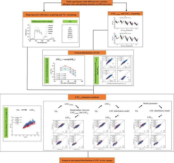
Three methods were used to estimate the LNCLi: (1) estimating the LNCCanopy by VIs and then estimating the LNCLi based on the relationship between the LNCLi and LNCCanopy; (2) estimating the LNC in any leaf layer of the rice canopy by VIs, inputting the results into the LNC vertical distribution model [Eqn (5)] to obtain the model parameters, and then estimating the LNCLi by the LNC vertical distribution model; and (3) estimating the model parameters by using VIs directly and then estimating the LNCLi by the LNC vertical distribution model. Figure 1 shows the main steps for the whole procedure.
Figure 1.
Flowchat for establishing the optimal LNCLi estimation model.
Results
Temporal and Spatial Distribution Characteristics of the LNC in the Rice Canopy
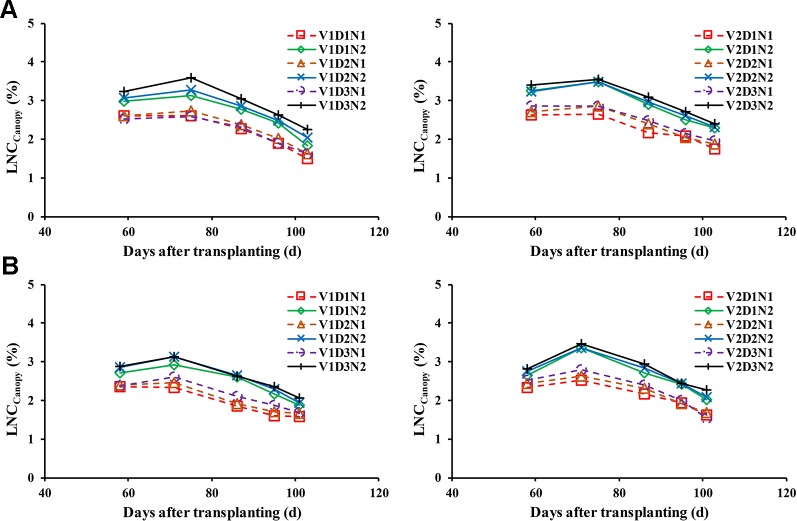
Changes of the LNCCanopy during whole growth stages in different treatments and years are shown in Figure 2. The results showed that the LNCCanopy decrease with increases in the days after transplanting in all treatments when the effect of nitrogen fertilizer application was neglected, which caused the LNCCanopy to increase slightly.
Figure 2.
Changes of the LNCCanopy during the whole growth stages under different treatment in 2015 (A) and 2016 (B). Jointing fertilizer was applied at approximately 60 days after transplanting (DAT).
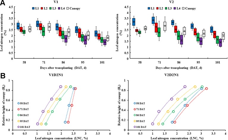
The data distribution characteristics of the LNCLi and LNCCanopy at different growth periods (Figure 3A) indicated that the values of the LNCL2 and LNCCanopy are similar in all treatments during whole growth stages. Compared with V1, there were significant differences between the LNCL1 and LNCL4 in V2. The LNC presented a decreasing trend from top to bottom within the rice canopy, and the LNC of each leaf layer decreased along with the days after transplanting (Figure 3B).
Figure 3.
Data distribution characteristics of the LNCLi and LNCCanopy at different growth period in 2015 (A) and the vertical distribution characteristics of the LNC in rice canopy, take V1D1N1 and V2D1N1 for example (B).
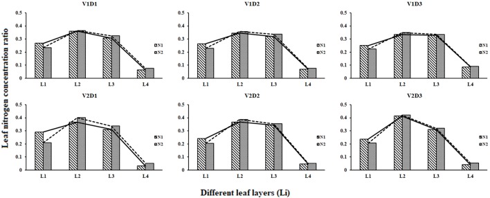
The leaf N concentration ratio of each leaf layer changed little in different treatments during whole growth stages (Figure 4). The LNCR2 was the highest (0.34 – 0.37 for V1, and 0.38 – 0.43 for V2), and the LNCR4 was the lowest (0.06 – 0.09 for V1, and 0.03 – 0.05 for V2). The differences among the LNCR between high N rates and low N rates decreased as the planting densities decreased.
Figure 4.
Leaf nitrogen concentration ratio of different leaf layers under different treatments (2015).
Relationships of LNCCanopy With LNCLi and LNCALi
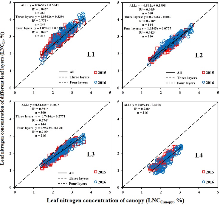
The LNC of the middle and upper leaf layers had a closer relationship with the LNCCanopy than that of the lower leaf layer (Figure 5). The LNCL1 (upper leaf layer) was significantly higher than the LNCCanopy, whereas the LNCL3 and LNCL4 (lower leaf layer) were lower than the LNCCanopy. Overall, the relationship between the LNCLi and LNCCanopy was stable over the years.
Figure 5.
Relationship between the LNCLi and LNCCanopy. * means accurate to 0.001.
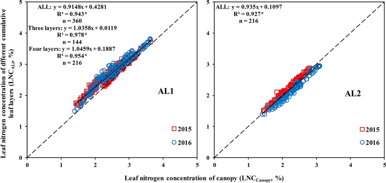
A good correlation was observed between the LNCALi and LNCCanopy, and the coefficient of determination (R2) could reach more than 0.9 (Figure 6). The LNCAL2 could best represent the LNCCanopy when the canopy was divided into three leaf layers, which indicated that from top to bottom, 67% of the canopy can represent the whole canopy. The LNCAL3 could represent the LNCCanopy best when the canopy was divided into four leaf layers, which demonstrated that from top to bottom, 75% of the canopy can represent the whole canopy.
Figure 6.
Relationship between the LNCALi and LNCCanopy. * means accurate to 0.001.
Effects of Different N Rates and Planting Densities on the LNCLi
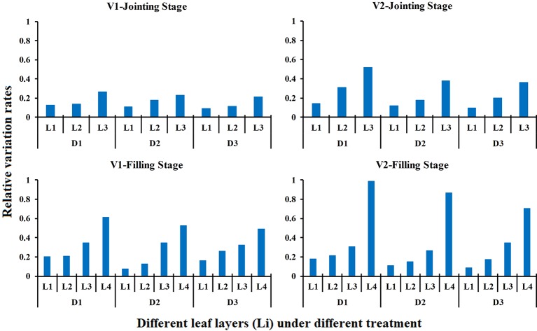
The effects of different N rates and planting densities on the LNCLi in different growth stages are shown in Figure 7. The results indicated that the effect of different N rates on the LNC of each leaf layer increased from the top to the bottom of the canopy, and the bottom leaf layer (L3) was most affected by the N application level at the jointing stage. Similar rules were found during the filling stage, and the impact increased slightly. The bottom leaf layer (L4) was still the leaf layer that was most affected by the N rate. The effects of different N rates on the LNCLi did not differ between the two rice varieties. Compared with N rate, planting densities has less effect on LNCLi. For the same variety and the same growth period, the relative variation rates of LNC in middle and upper leaf layers remained stable under varied planting densities. However, the relative variation rates of LNC in the bottom leaf layer decreased gradually with decreased planting densities.
Figure 7.
Relative variation rate of the LNCLi in response to different N rates in different growth stage (2015). The relative variation rate is the product of the nitrogen traits under high nitrogen treatment minus the nitrogen traits under low nitrogen treatment over the nitrogen traits under low nitrogen treatment.
LNC Vertical Distribution Model Verification and Parameter Acquisition
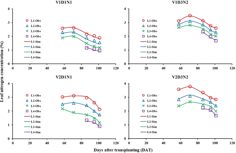
The measured LNCLi values in two field experiments were used to test the LNC vertical distribution model (Figure 8) and obtain the model parameters (Table 1). The results showed that the LNCLi could be better simulated in different varieties, treatments, and growth stages by using the LNC vertical distribution model proposed in this study (average R2 is higher than 0.97).
Figure 8.
Comparison of simulated (Sim) and observed (Obs) distribution of leaf nitrogen concentration in rice canopy (take V1D1N1, V1D3N2, V2D1N1, and V2D3N2 for example).
Table 1.
Basic statistics of the parameters of the vertical distribution of the leaf nitrogen content model.
| V1 | V2 | ||||||||
|---|---|---|---|---|---|---|---|---|---|
| Mean | SD | Min. | Max. | Mean | SD | Min. | Max. | ||
| Three layers | a | 2.2381 | 0.3485 | 1.6980 | 2.9680 | 2.0415 | 0.3893 | 1.3420 | 2.7050 |
| b | 0.3947 | 0.1017 | 0.2074 | 0.6435 | 0.6475 | 0.1874 | 0.2652 | 1.0580 | |
| R2 | 0.9787 | 0.0201 | 0.9093 | 1.0000 | 0.9826 | 0.0194 | 0.9147 | 1.0000 | |
| RMSE | 0.0657 | 0.0406 | 0.0001 | 0.1550 | 0.0914 | 0.0688 | 0.0007 | 0.2890 | |
| Four layers | a | 1.5368 | 0.3771 | 0.8923 | 2.3370 | 1.3746 | 0.3905 | 0.7599 | 2.2010 |
| b | 0.6709 | 0.1472 | 0.3154 | 0.9497 | 0.9360 | 0.2340 | 0.4877 | 1.3870 | |
| R2 | 0.9713 | 0.0235 | 0.9008 | 0.9991 | 0.9831 | 0.0143 | 0.9299 | 1.0000 | |
| RMSE | 0.0788 | 0.0405 | 0.0117 | 0.2201 | 0.0941 | 0.0492 | 0.0027 | 0.2487 | |
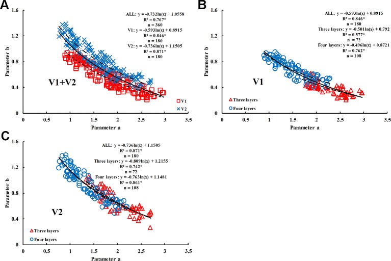
The range of values of model parameters “a” and “b” was slightly different between the rice varieties and different growth stages. In the same period, the parameter “a” of V1 was higher than that of V2, with the value ranging between 1.6980 and 2.9680; however, the parameter “b” of V1 was lower than that of V2, with the value ranging between 0.2074 and 0.6435. The value of parameter “a” decreased as the growth period advanced; however, the value of parameter “b” increased. Parameter “a” was well correlated with parameter “b” in the two rice varieties (R2 values were 0.84 and 0.87, respectively) and decreased as parameter “b” increased.
Relationships of the VIs With LNCLi and Parameter “a”
The relationship between the LNCLi and VIs was tested (Tables 2, 3, 4), and the results showed that the VIs could estimate the LNCCanopy and were well correlated with the LNCLi. The estimation accuracy of the VIs for the LNCCanopy, LNCL1, LNCL2, LNCL3, and LNCL4 decreased in turn, and the corresponding optimal VIs were the NDDA (R2 = 0.684), NDRE (R2 = 0.631), NDRE (R2 = 0.589), RVI (R2 = 0.516), and RVI (R2 = 0.507) when combined for the two rice varieties. The relationship between VIs and LNCLi did not change significantly between years (Table 3); the estimation accuracy of a single year was better than those of two years. In addition, the optimal VIs for estimating LNC of each leaf layer was basically unchanged. Different VIs showed varied change modes in different planting densities (Table 4). At the high planting density, VIs showed the highest accuracy in estimating LNCCanopy and LNCLi. However, the estimation accuracy of some VIs (e.g. RDVI, NDRE, and MTVI2) decreased gradually, while other VIs (e.g. RVI, NDVI and CI) decreased first and then increased at medium and low planting densities.
Table 2.
Coefficients of determination (R2) for the relationship between the vegetation indices and the leaf nitrogen concentration in different rice cultivars.
| LNCCanopy | LNCL1 | LNCL2 | LNCL3 | LNCL4 | |||||||||||
|---|---|---|---|---|---|---|---|---|---|---|---|---|---|---|---|
| V1 | V2 | V1+V2 | V1 | V2 | V1+V2 | V1 | V2 | V1+V2 | V1 | V2 | V1+V2 | V1 | V2 | V1+V2 | |
| RVI | 0.61 | 0.73 | 0.67 | 0.58 | 0.70 | 0.59 | 0.57 | 0.56 | 0.56 | 0.55 | 0.54 | 0.52 | 0.65 | 0.50 | 0.51 |
| NDVI | 0.43 | 0.69 | 0.54 | 0.56 | 0.72 | 0.65 | 0.55 | 0.57 | 0.57 | 0.30 | 0.51 | 0.33 | 0.32 | 0.40 | 0.25 |
| CI | 0.66 | 0.72 | 0.68 | 0.64 | 0.70 | 0.62 | 0.62 | 0.53 | 0.58 | 0.53 | 0.52 | 0.49 | 0.62 | 0.49 | 0.48 |
| OSAVI | 0.13 | 0.17 | 0.15 | 0.16 | 0.18 | 0.27 | 0.16 | 0.18 | 0.16 | 0.07 | 0.23 | 0.07 | 0.06 | 0.36 | 0.05 |
| NDRE | 0.65 | 0.73 | 0.68 | 0.65 | 0.72 | 0.63 | 0.63 | 0.56 | 0.59 | 0.54 | 0.53 | 0.50 | 0.63 | 0.48 | 0.45 |
| SIPI | 0.18 | 0.61 | 0.35 | 0.31 | 0.66 | 0.48 | 0.31 | 0.54 | 0.43 | 0.13 | 0.44 | 0.20 | 0.21 | 0.32 | 0.18 |
| MTVI2 | 0.11 | 0.15 | 0.13 | 0.12 | 0.17 | 0.25 | 0.13 | 0.17 | 0.40 | 0.05 | 0.22 | 0.05 | 0.03 | 0.33 | 0.03 |
| MCARI | 0.49 | 0.43 | 0.33 | 0.36 | 0.38 | 0.15 | 0.39 | 0.23 | 0.22 | 0.51 | 0.25 | 0.32 | 0.40 | 0.02 | 0.17 |
| TCARI | 0.39 | 0.48 | 0.36 | 0.42 | 0.49 | 0.22 | 0.42 | 0.33 | 0.28 | 0.45 | 0.28 | 0.32 | 0.35 | 0.04 | 0.14 |
| NDDA | 0.67 | 0.71 | 0.68 | 0.63 | 0.69 | 0.60 | 0.62 | 0.53 | 0.57 | 0.55 | 0.52 | 0.51 | 0.66 | 0.49 | 0.50 |
| R705/(R717+R491) | 0.70 | 0.65 | 0.66 | 0.63 | 0.59 | 0.58 | 0.63 | 0.42 | 0.52 | 0.56 | 0.45 | 0.47 | 0.42 | 0.47 | 0.30 |
| TBDR | 0.57 | 0.70 | 0.62 | 0.55 | 0.64 | 0.53 | 0.55 | 0.50 | 0.52 | 0.52 | 0.51 | 0.48 | 0.56 | 0.50 | 0.43 |
| MCARI/MTVI2 | 0.66 | 0.60 | 0.58 | 0.57 | 0.56 | 0.41 | 0.56 | 0.37 | 0.41 | 0.66 | 0.41 | 0.52 | 0.59 | 0.26 | 0.41 |
| TCARI/OSAVI | 0.52 | 0.59 | 0.50 | 0.51 | 0.59 | 0.36 | 0.50 | 0.40 | 0.38 | 0.58 | 0.36 | 0.45 | 0.40 | 0.12 | 0.25 |
The results were accurate to 0.01.
Table 3.
Coefficients of determination (R2) for the relationship between the vegetation indices and the leaf nitrogen concentration in different years.
| LNCCanopy | LNCL1 | LNCL2 | LNCL3 | LNCL4 | ||||||
|---|---|---|---|---|---|---|---|---|---|---|
| 2015 | 2016 | 2015 | 2016 | 2015 | 2016 | 2015 | 2016 | 2015 | 2016 | |
| RVI | 0.74 | 0.70 | 0.81 | 0.61 | 0.68 | 0.58 | 0.67 | 0.54 | 0.61 | 0.56 |
| NDVI | 0.47 | 0.60 | 0.59 | 0.56 | 0.55 | 0.56 | 0.38 | 0.30 | 0.37 | 0.27 |
| CI | 0.72 | 0.74 | 0.81 | 0.69 | 0.64 | 0.62 | 0.53 | 0.54 | 0.52 | 0.46 |
| OSAVI | 0.32 | 0.25 | 0.56 | 0.51 | 0.33 | 0.26 | 0.16 | 0.01 | 0.16 | 0.01 |
| NDRE | 0.72 | 0.72 | 0.82 | 0.66 | 0.66 | 0.61 | 0.54 | 0.53 | 0.54 | 0.44 |
| SIPI | 0.27 | 0.32 | 0.35 | 0.24 | 0.41 | 0.38 | 0.18 | 0.12 | 0.24 | 0.09 |
| MTVI2 | 0.27 | 0.25 | 0.12 | 0.13 | 0.28 | 0.16 | 0.13 | 0.01 | 0.11 | 0.00 |
| MCARI | 0.34 | 0.35 | 0.53 | 0.37 | 0.23 | 0.28 | 0.22 | 0.21 | 0.12 | 0.20 |
| TCARI | 0.31 | 0.40 | 0.55 | 0.37 | 0.25 | 0.30 | 0.25 | 0.24 | 0.14 | 0.15 |
| NDDA | 0.74 | 0.74 | 0.82 | 0.68 | 0.65 | 0.62 | 0.57 | 0.56 | 0.53 | 0.49 |
| R705/(R717+R491) | 0.67 | 0.71 | 0.65 | 0.54 | 0.51 | 0.59 | 0.42 | 0.46 | 0.30 | 0.31 |
| TBDR | 0.67 | 0.63 | 0.72 | 0.59 | 0.63 | 0.49 | 0.57 | 0.50 | 0.51 | 0.49 |
| MCARI/MTVI2 | 0.64 | 0.63 | 0.41 | 0.54 | 0.47 | 0.47 | 0.51 | 0.47 | 0.42 | 0.43 |
| TCARI/OSAVI | 0.48 | 0.51 | 0.32 | 0.43 | 0.39 | 0.37 | 0.41 | 0.38 | 0.27 | 0.24 |
The results were accurate to 0.01.
Table 4.
Coefficients of determination (R2) for the relationship between the vegetation indices and the leaf nitrogen concentration in different planting densities.
| LNCCanopy | LNCL1 | LNCL2 | LNCL3 | LNCL4 | |||||||||||
|---|---|---|---|---|---|---|---|---|---|---|---|---|---|---|---|
| D1 | D2 | D3 | D1 | D2 | D3 | D1 | D2 | D3 | D1 | D2 | D3 | D1 | D2 | D3 | |
| RVI | 0.77 | 0.63 | 0.69 | 0.65 | 0.55 | 0.62 | 0.69 | 0.51 | 0.54 | 0.61 | 0.55 | 0.58 | 0.62 | 0.46 | 0.49 |
| RDVI | 0.70 | 0.60 | 0.55 | 0.73 | 0.63 | 0.68 | 0.66 | 0.58 | 0.57 | 0.47 | 0.45 | 0.38 | 0.36 | 0.24 | 0.25 |
| NDVI | 0.78 | 0.66 | 0.70 | 0.68 | 0.58 | 0.65 | 0.69 | 0.54 | 0.53 | 0.60 | 0.55 | 0.56 | 0.58 | 0.45 | 0.48 |
| CI | 0.32 | 0.04 | 0.24 | 0.49 | 0.11 | 0.38 | 0.32 | 0.06 | 0.29 | 0.16 | 0.02 | 0.12 | 0.19 | 0.00 | 0.08 |
| OSAVI | 0.78 | 0.67 | 0.70 | 0.69 | 0.59 | 0.67 | 0.71 | 0.55 | 0.55 | 0.61 | 0.57 | 0.57 | 0.58 | 0.45 | 0.47 |
| NDRE | 0.54 | 0.38 | 0.37 | 0.61 | 0.44 | 0.51 | 0.55 | 0.41 | 0.45 | 0.34 | 0.29 | 0.25 | 0.31 | 0.19 | 0.20 |
| SIPI | 0.28 | 0.03 | 0.22 | 0.45 | 0.10 | 0.34 | 0.28 | 0.05 | 0.25 | 0.13 | 0.01 | 0.10 | 0.16 | 0.01 | 0.05 |
| MTVI2 | 0.39 | 0.33 | 0.26 | 0.18 | 0.16 | 0.12 | 0.29 | 0.22 | 0.13 | 0.36 | 0.36 | 0.34 | 0.06 | 0.28 | 0.17 |
| MCARI | 0.41 | 0.40 | 0.35 | 0.24 | 0.24 | 0.24 | 0.36 | 0.30 | 0.22 | 0.35 | 0.42 | 0.39 | 0.05 | 0.29 | 0.15 |
| TCARI | 0.78 | 0.66 | 0.69 | 0.67 | 0.56 | 0.63 | 0.68 | 0.53 | 0.52 | 0.62 | 0.56 | 0.57 | 0.60 | 0.46 | 0.50 |
| NDDA | 0.76 | 0.68 | 0.65 | 0.63 | 0.56 | 0.61 | 0.63 | 0.51 | 0.45 | 0.53 | 0.53 | 0.48 | 0.35 | 0.32 | 0.33 |
| R705/(R717+R491) | 0.76 | 0.62 | 0.61 | 0.67 | 0.48 | 0.53 | 0.69 | 0.49 | 0.45 | 0.57 | 0.57 | 0.54 | 0.52 | 0.50 | 0.39 |
| TBDR | 0.67 | 0.56 | 0.54 | 0.47 | 0.38 | 0.41 | 0.55 | 0.41 | 0.34 | 0.55 | 0.54 | 0.53 | 0.43 | 0.45 | 0.40 |
| MCARI/MTVI2 | 0.56 | 0.52 | 0.49 | 0.49 | 0.35 | 0.40 | 0.48 | 0.39 | 0.34 | 0.44 | 0.51 | 0.48 | 0.16 | 0.36 | 0.24 |
| TCARI/OSAVI | 0.77 | 0.63 | 0.69 | 0.65 | 0.55 | 0.62 | 0.69 | 0.51 | 0.54 | 0.61 | 0.55 | 0.58 | 0.62 | 0.46 | 0.49 |
The result were accurate to 0.01.
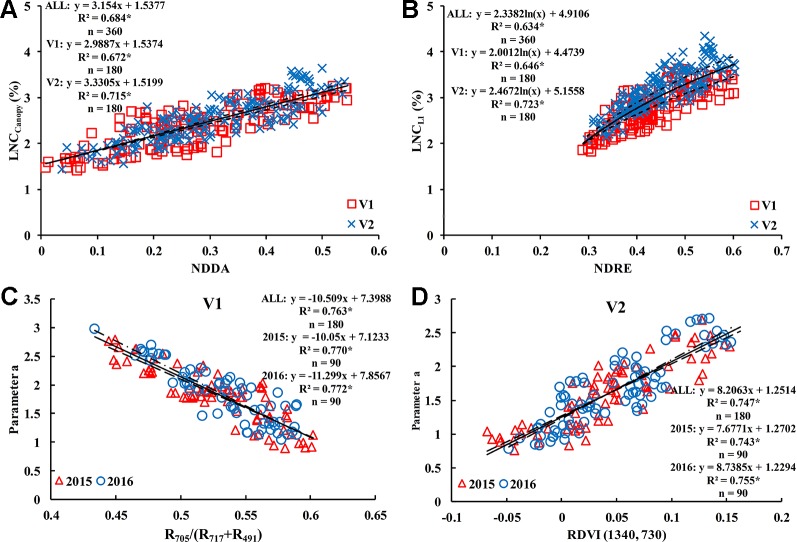
There were some differences in VIs for different rice cultivars. For V1, the optimal vegetation index for estimating the LNCCanopy was R705/(R717+R491) (R2 = 0.704); NDRE was the best vegetation index for LNCL1 estimation with the highest value (0.646) of R2; R705/(R717+R491) also performed best in the estimation of LNCL2 (R2 = 0.631); and the optimal VIs for estimating LNCL3 and LNCL4 were MCARI/MTVI2 (R2 = 0.563) and NDDA (R2 = 0.627), respectively. For V2, NDRE performed best in estimating LNCCanopy and LNCL1, with R2 values of 0.728 and 0.723, respectively; the optimal vegetation index for estimating LNCL2 was NDVI (R2 = 0.574); RVI performed best in estimating LNCL3 and LNCL4, with R2 values of 0.541 and 0.501, respectively. Due to the high accuracy and stability between different treatments, NDDA and NDRE were selected to estimate LNCCanopy (Figure 10A) and LNCL1 (Figure 10B) and were used in the construction of methods 1 and 2 in Section 2.5.
Figure 10.
Optimum vegetation indices for estimating LNCCanopy (A), LNCL1 (B), and parameter “a” [(C) is V1 and (D) is V2]. * means accurate to 0.001.
Due to the good correlation between parameter “a” and parameter “b” (Figure 9A–C), and the difference in the correlation for different rice varieties, four representative two-band VIs (DI, SR, NDVI, and RDVI) were selected to conduct the 350 nm–1500 nm sensitivity analyses of parameter “a.” The results showed that R705/(R717+R491) and RDVI (1340, 730) were suitable for the estimation of parameter “a” in V1 (R2 = 0.763) (Figure 10C) and V2 (R2 = 0.747) (Figure 10D), respectively. Based on these results, parameter “b” could be obtained by the relationship between parameter “a” and “b”.
Figure 9.
Relationship between parameter ‘a' and ‘b' in different rice varieties. (A) V1+V2, (B) V1, and (C) V2. * means accurate to 0.001.
LNCLi Estimation of Rice Canopy
The following three methods were compared for estimating the LNCLi within the rice canopy:
(1) estimate the LNCCanopy by the NDDA (Figure 10A) and then estimate the LNCLi based on the relationship between the LNCLi and LNCCanopy (Figure 5):
| (6) |
| (7) |
| (8) |
| (9) |
| (10) |
(2) estimate the LNCL1 by the NDRE (Figure 10B), input the results into the LNC vertical distribution model to obtain the model parameters, and then estimate the LNCLi by the LNC vertical distribution model:
| (11) |
| (12) |
| (13) |
| (5) |
(3) directly estimate the model parameters using R705/(R717+R491) (Figure 10C) and RDVI (1340, 730) (Figure 10D) and then estimate the LNCLi by the LNC vertical distribution model:
| (14) |
| (13) |
| (5) |
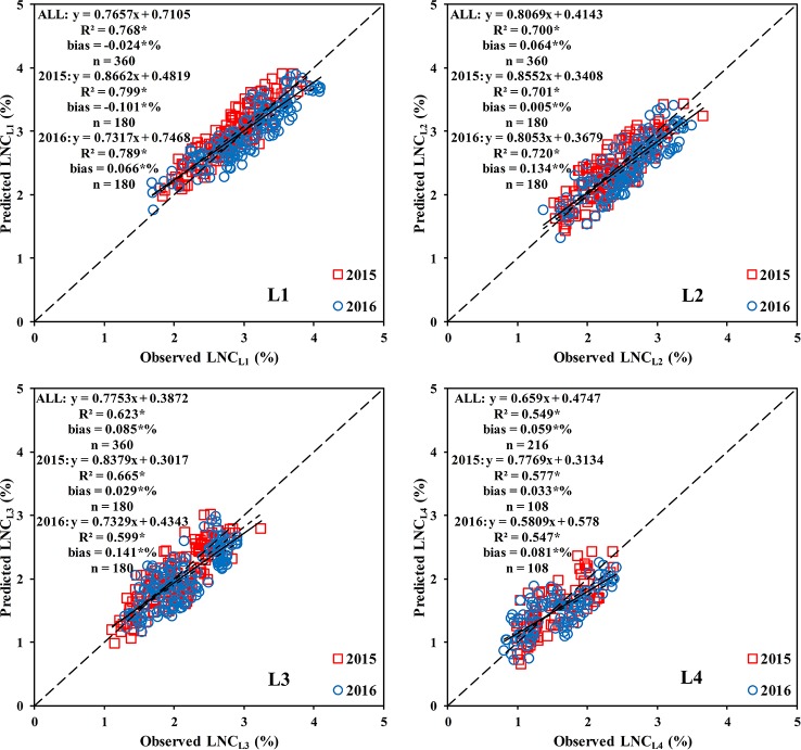
The results (Figure 11 and Supplementary Figures 3 and 4) showed that all three methods could estimate the LNCLi within the rice canopy; however, method 1 significantly underestimated the LNCL1. The methods (2 and 3) that combined the LNC vertical distribution model performed better in estimating the LNCLi. Method 2 was the optimal method for estimating the LNCL1, LNCL2, LNCL3, and LNCL4, which had R2 values of 0.768, 0.700, 0.623, and 0.549, respectively.
Figure 11.
Comparison between the observed and predicted LNC in different leaf layers based on method 2. * means accurate to 0.001.
Discussion
In this study, the temporal and spatial distribution characteristics of the LNC in the rice canopy at different growth stages were investigated. Our study results showed that the LNC distribution followed a declining trend from the top layer to the bottom layer in rice canopy (Figure 3), which is consistent with the findings in wheat (Li et al., 2015; Zhao et al., 2017), winter oilseed rape (Li et al., 2018), and maize (Ye et al., 2018). Light conditions are the main limiting factors for vegetation photosynthesis, with more N allocated to leaves receiving higher light intensities (Wyka et al., 2012); thus, the top of the canopy, which has the best light conditions in the rice canopy, is assigned more. N. Chen et al. (2014) reported the light use efficiency (LUE) is lower in the bottom leaf layers than the top fresh leaf layers because the lower leaves of the canopy are more sensitive to nutrient stress and senescence. Therefore, the LNC and LNCR were the lowest in the bottom leaf layer of the rice canopy (Figures 3 and 4). In the high N treatments (N2), L2 and L3 had higher LAI and more sunlit leaves compared with the low N treatment, which led to a higher LNCL1 and a lower LNCR1 in the high N treatments than those in the low N treatments (Figure 4). In the low planting density (D3), the plant spacing is larger than the high planting density, and more light can reach the lower leaf layer of rice canopy. Therefore, compared with high density treatments, low density treatments distributed more N in the lower leaf layer of the rice canopy. These may explain why the relative variation rates of LNC decreased gradually with the decreased planting densities for the bottom leaf layer of the canopy (Figure 7). V1 (with erect leaf) and V2 (with spread leaf) performed differently, and the leaves of V2 were mainly concentrated in the upper layer of the canopy, causing less light in the lower part of the canopy. Therefore, for V2, the vertical distribution trend of N was steeper and the low density treatment increased the LNC of lower leaf layers more significantly.
Due to the transferability of N (Wang et al., 2005), the N of the bottom leaf layer is transferred to the top leaf layer when the N supply is limited (Wang et al., 2006). Therefore, the upper layers were less affected by the N rates, and N stress was more obvious in the lower layers, which is similar to the findings of Huang et al. (2014). Kong et al. (2017) also showed that accurate estimations of the physiological and biochemical parameters of the bottom leaves can facilitate the early detection of subtle changes in the field. Studies also showed that the nitrogen stress index (NSI) and the nitrogen spectral stress index (NSSI) of the bottom two leaves could indicate the N stress in maize (Lu et al., 2018). D'Odorico et al. (2019) reported that bottom leaves showed higher photosynthetic efficiency at low light levels and were the main contributor to total canopy photosynthesis until the start of senescence. The LNC of the bottom leaf layer was significantly lower than the LNCCanopy, and the LNCCanopy was mainly affected by the LNC of the upper and middle leaf layers (Figures 5 and 6). Therefore, the LNCCanopy could not rapidly show whether crops were under N stress, which indicates the importance of accurately estimating the LNC of each layer within the canopy.
The LNC vertical distribution model proposed in this study could simulate the vertical distribution of the LNC within the rice canopy (Table 1). The difference in light distribution caused by differences in the canopy structure (e.g., LAI and leaf angle) is the main reason for the non-uniform N distribution (Archontoulis et al., 2011; Hikosaka et al., 2016; Ye et al., 2018), and the relationship between the N distribution and light distribution differs at different growth stages (Dreccer et al., 2000). Therefore, the parameters of our model were susceptible to the growth period and rice variety (Table 1).
Previous studies seldom considered the vertical distribution of N within the canopy (Li et al., 2016). Our studies showed that the estimation accuracy of LNCLi based on VIs decreased as the depth of the canopy increased, and the upper and middle layers were the effective leaf layers for LNC predictions using VIs. This finding is consistent with the results of Li et al. (2018) in the winter oilseed rape. Luo et al. (2016) reported that the spectral reflectance of the crop canopy is mainly affected by the upper layer in the visible and near-infrared bands, which may explain why the VIs (e.g., SIPI) based on red and near-infrared bands are less effective at estimating the LNC of the bottom leaf layers. VIs that include the red edge band showed a close correlation with the LNC of different leaf layers, which is consistent with the findings of Zhao et al. (2017) in winter wheat. The RVI (780, 740), which was proposed to estimate N absorption in different maize leaf layers (Winterhalter et al., 2012), performed well in estimating the LNC of the lower leaf layer in the rice canopy; however, it did not perform stably between different rice varieties. Canopy structure, physiological and biochemical characteristics of target objects, and background affect the estimation accuracy of VIs by affecting canopy reflectance (Zarco-Tejada et al., 2001). The physiological and biochemical characteristics of crops and the size of soil and water background are mainly affected by N rates and planting density. The higher the proportion of vegetation signal in canopy reflectance, the higher the accuracy of VIs in estimating physiological and biochemical status of vegetation. Therefore, VIs showed a high accuracy in LNCCanopy and LNCLi estimation under the high planting density (Table 4). Under the same N rates, the N obtained by a single plant increased with the decreased planting density. At the same time, the proportion of background and the size of individual vegetation canopy were constantly changing, which was a complex process. As a result, the VIs that are sensitive to canopy structure had different change modes compared with the VIs that are sensitive to leaf color. The canopy reflectance is bidirectional, and different canopy structures often lead to different variations of canopy reflectance (Li et al., 2015; Zhao et al., 2017). Different rice varieties have various plant types and leaf angles, which affected the canopy structure and also changed the N vertical distribution gradient. Therefore, VIs have significant differences between the two rice cultivars (Table 2).
The accuracy of estimating the LNCLi by VIs is limited due to the inconsistency of the optimal VIs and optimal band range among different leaf layers within the canopy, and different remote sensing models must be developed for different layers, although such models are difficult to apply in practice. Therefore, three methods for estimating the LNCLi were constructed and compared in this paper (Section 2.5). Method 1 had a significant underestimation of the LNCL1 and performed poorer than methods 2 and 3, which combine the LNC vertical distribution model for estimating the LNCLi. Method 3 is subject to the empirical relationship between parameter “a” and the VIs, and it is greatly influenced by external factors (e.g., varieties). Compared with methods 1 and 2, the universality of method 3 must be validated using additional data. Method 2 only needs to accurately estimate the LNC of any leaf layer within the canopy, and the results are then combined with the LNC vertical distribution model, which is a high-precision method with few input parameters and easy calculation, and it allows the LNC at any height of the canopy to be obtained with higher precision. Therefore, it is the optimal choice for obtaining the vertical distribution of the LNC within the rice canopy because it estimates the LNCL1 and combines it with the LNC vertical distribution model.
Conclusion
In the present study, we investigated the vertical distribution characteristics of the LNC within the rice canopy and the relationships of the LNCCanopy with the LNCLi and LNCALi and proposed an LNC vertical distribution model based on the relative canopy height. The performance of multiple VIs in the LNCLi and model parameter “a” estimation was evaluated at different growth stages. We also compared the three methods for estimating the LNC in different leaf layers within the rice canopy. The results demonstrated that the LNC presented a decreasing trend from top to bottom within the rice canopy, the LNC in the bottom of rice canopy was more susceptible to different N rates, and the LNCLi could be better simulated in different varieties, treatments, and growth stages by using the LNC vertical distribution model. The NDRE could accurately estimate the LNCL1, and in combination with the LNC vertical distribution model, the parameters of the model could be accurately obtained, which promotes more accurate estimations of the LNCLi during the whole growth period. The results provide technical support for predicting the spatial and temporal LNC distribution of rice.
Data Availability Statement
The datasets generated for this study are available on request to the corresponding author.
Author Contributions
JH and YT conceived and designed the experiments. XZ, WG, and YP performed the experiments. JH analyzed the data. JH and YT wrote the original manuscript. YT, XY, TC, YZ, and WC reviewed and edited the original manuscript.
Funding
This work was supported by the National Natural Science Foundation of China (31971784), the National Key R&D Program (2018YFD0300805), and the Priority Academic Program Development of Jiangsu Higher Education Institutions (PAPD).
Conflict of Interest
The authors declare that the research was conducted in the absence of any commercial or financial relationships that could be construed as a potential conflict of interest.
Acknowledgments
We would like to thank Yehui Qin, Liyun Zhao, and Xiang Zhou for their help with field data collection. We are grateful to the constructive suggestions provided by three anonymous reviewers.
Supplementary Material
The Supplementary Material for this article can be found online at: https://www.frontiersin.org/articles/10.3389/fpls.2019.01802/full#supplementary-material
Abbreviations
Ali, The ith accumulative leaf layer; CIred edge, Chlorophyll index red-edge; DW, The dry weight; Hr, The relative canopy height; Li, The ith leaf layer; LAI, Leaf area index; LDW, Leaf dry weight; LNC, Leaf nitrogen concentration; LNCCanopy, LNC of the canopy; LNCLi, LNC of the ith leaf layer; LNCR, LNC ratio; LNCRi, LNC ratio of the ith leaf layer; LND, Leaf nitrogen density; LUE, Light use efficiency; MCARI, Modified chlorophyll absorption in reflectance index; MTVI2, Modified triangular vegetation index 2; N, Nitrogen; NL, Nitrogen content per unit leaf area; NDDA, Normalized difference index of the double-peak areas; NDRE, Normalized difference red-edge; NDVI, Normalized difference vegetation index; NSI, Nitrogen stress index; NSSI, Nitrogen spectral stress index; OSAVI, Optimized soil adjusted vegetation index; R2, Determination coefficient; RDVI, Renormalized difference vegetation index; RMSE, Root mean square error; RVI, Ratio vegetation index; SIPI, Structure intensive pigment index; TBDR, Three-band difference ratio; TCARI, Transformed chlorophyll absorption ratio index; Vis, Vegetation indices; ZD, The depth from top of canopy.
References
- Aerts R., Chapin F. S. (1999). The mineral nutrition of wild plants revisited: a re-evaluation of processes and patterns. Adv. Ecol. Res. 30, 1–67. 10.1016/S0065-2504(08)60016-1 [DOI] [Google Scholar]
- Anten N. P. R., Werger M. J. A., Medina E. (1998). Nitrogen distribution and leaf area indices in relation to photosynthetic nitrogen use efficiency in savanna grasses. Plant Ecol. 138, 67–75. 10.1023/A:1009727822617 [DOI] [Google Scholar]
- Archontoulis S. V., Vos J., Yin X., Bastiaans L., Danalatos N. G., Struik P. C. (2011). Temporal dynamics of light and nitrogen vertical distributions in canopies of sunflower, kenaf and cynara. F. Crop Res. 122, 186–198. 10.1016/j.fcr.2011.03.008 [DOI] [Google Scholar]
- Barnes E. M., Clarke T. R., Richards S. E., Colaizzi P. D., Haberland J., Kostrzewski M., et al. (2000). Coincident detection of crop water stress, nitrogen status and canopy density using ground based multispectral data, in: Bloomington, MN, USA: Proc. 5th Int. Conf. Precis Agric. [Google Scholar]
- Bertheloot J., Andrieu B., Martre P. (2012). Light-nitrogen relationships within reproductive wheat canopy are modulated by plant modular organization. Eur. J. Agron. 42, 11–21. 10.1016/j.eja.2012.03.005 [DOI] [Google Scholar]
- Chemura A., Mutanga O., Odindi J., Kutywayo D. (2018). Mapping spatial variability of foliar nitrogen in coffee (Coffea arabica L.) plantations with multispectral Sentinel-2 MSI data. ISPRS J. Photogramm. Remote Sens. 138, 1–11. 10.1016/j.isprsjprs.2018.02.004 [DOI] [Google Scholar]
- Chen J., Reynolds J. F., Harley P. C., Tenhunen J. D. (1993). Coordination theory of leaf nitrogen distribution in a canopy. Oecologia 93, 63–69. 10.1007/BF00321192 [DOI] [PubMed] [Google Scholar]
- Chen T., Henke M., De Visser P. H. B., Buck-Sorlin G., Wiechers D., Kahlen K., et al. (2014). What is the most prominent factor limiting photosynthesis in different layers of a greenhouse cucumber canopy? Ann. Bot. 114, 677–688. 10.1093/aob/mcu100 [DOI] [PMC free article] [PubMed] [Google Scholar]
- Ciganda V. S., Gitelson A. A., Schepers J. (2012). How deep does a remote sensor sense? Expression of chlorophyll content in a maize canopy. Remote Sens. Environ. 126, 240–247. 10.1016/j.rse.2012.08.019 [DOI] [Google Scholar]
- Coble A. P., Cavaleri M. A. (2015). Light acclimation optimizes leaf functional traits despite height-related constraints in a canopy shading experiment. Oecologia 177, 1131–1143. 10.1007/s00442-015-3219-4 [DOI] [PubMed] [Google Scholar]
- D'Odorico P., Emmel C., Revill A., Liebisch F., Eugster W., Buchmann N. (2019). Vertical patterns of photosynthesis and related leaf traits in two contrasting agricultural crops. Funct. Plant Biol. 46, 213–227. 10.1071/FP18061 [DOI] [PubMed] [Google Scholar]
- Dreccer M. F., Van Oijen M., Schapendonk A. H. C. M., Pot C. S., Rabbinge R. (2000). Dynamics of vertical leaf nitrogen distribution in a vegetative wheat canopy. Impact on canopy photosynthesis. Ann. Bot. 86, 823–831. 10.1006/anbo.2000.1244 [DOI] [Google Scholar]
- Gara T. W., Darvishzadeh R., Skidmore A. K., Wang T. (2018). Impact of vertical canopy position on leaf spectral properties and traits across multiple species. Remote Sens. 10, 346. 10.3390/rs10020346 [DOI] [Google Scholar]
- Gastal F., Lemaire G. (2002). N uptake and distribution in crops: An agronomical and ecophysiological perspective. J. Exp. Bot. 53, 789–799. 10.1093/jexbot/53.370.789 [DOI] [PubMed] [Google Scholar]
- Gu J., Yin X., Stomph T. J., Struik P. C. (2014). Can exploiting natural genetic variation in leaf photosynthesis contribute to increasing rice productivity? A simulation analysis. Plant Cell Environ. 37, 22–34. 10.1111/pce.12173 [DOI] [PubMed] [Google Scholar]
- Gu J., Chen Y., Zhang H., Li Z., Zhou Q., Yu C., et al. (2017). Canopy light and nitrogen distributions are related to grain yield and nitrogen use efficiency in rice. F. Crop Res. 206, 74–85. 10.1016/j.fcr.2017.02.021 [DOI] [Google Scholar]
- He J., Zhang N., Su X., Lu J., Yao X., Cheng T., et al. (2019). Estimating leaf area index with a new vegetation index considering the influence of rice panicles. Remote Sens. 11, 1809. 10.3390/rs11151809 [DOI] [Google Scholar]
- Hikosaka K., Terashima I., Katoh S. (1994). Effects of leaf age, nitrogen nutrition and photon flux density on the distribution of nitrogen among leaves of a vine (Ipomoea tricolor Cav.) grown horizontally to avoid mutual shading of leaves. Oecologia 97, 451–457. 10.1007/BF00325881 [DOI] [PubMed] [Google Scholar]
- Hikosaka K., Anten N. P. R., Borjigidai A., Kamiyama C., Sakai H., Hasegawa T., et al. (2016). A meta-analysis of leaf nitrogen distribution within plant canopies. Ann. Bot. 118, 239–247. 10.1093/aob/mcw099 [DOI] [PMC free article] [PubMed] [Google Scholar]
- Hikosaka K. (2014). Optimal nitrogen distribution within a leaf canopy under direct and diffuse light. Plant Cell Environ. 37, 2077–2085. 10.1111/pce.12291 [DOI] [PubMed] [Google Scholar]
- Hirose T., Werger M. J. A. (1987). Maximizing daily canopy photosynthesis with respect to the leaf nitrogen allocation pattern in the canopy. Oecologia 72, 520–526. 10.1007/BF00378977 [DOI] [PubMed] [Google Scholar]
- Hirose T., Werger M. J. A., Pons T. L., van Rheenen J. W. A. (1988). Canopy structure and leaf nitrogen distribution in a stand of Lysimachia vulgaris L. as influenced by stand density. Oecologia 74, 145–150. 10.1007/BF00379180 [DOI] [PubMed] [Google Scholar]
- Huang W., Yang S., Pu R., Yang S. (2014). Estimation of nitrogen vertical distribution by Bi-Directional canopy reflectance in winter wheat. Sensors 14, 20347–20359. 10.3390/s141120347 [DOI] [PMC free article] [PubMed] [Google Scholar]
- Jia F., Liu G., Ding S., Yang Y., Fu Y., Wang Z. (2013). Using leaf spectral reflectance to monitor the effects of shading on nicotine content in tobacco leaves. Ind. Crops Prod. 51, 444–452. 10.1016/j.indcrop.2013.09.027 [DOI] [Google Scholar]
- Kattge J., Knorr W. (2007). Temperature acclimation in a biochemical model of photosynthesis: a reanalysis of data from 36 species. Plant Cell Environ. 30, 1176–1190. 10.1111/j.1365-3040.2007.01690.x [DOI] [PubMed] [Google Scholar]
- Kellomäki S., Wang K. Y. (1997). Effects of long-term CO2 and temperature elevation on crown nitrogen distribution and daily photosynthetic performance of Scots pine. For. Ecol. Manage. 99, 309–326. 10.1016/S0378-1127(97)00059-5 [DOI] [Google Scholar]
- Kong W., Huang W., Casa R., Zhou X., Ye H., Dong Y. (2017). Off-nadir hyperspectral sensing for estimation of vertical profile of leaf chlorophyll content within wheat canopies. Sensors 17, 2711. 10.3390/s17122711 [DOI] [PMC free article] [PubMed] [Google Scholar]
- Lemaire G., Onillon B., Gosse G., Chartier M., Allirand J. M. (1991). Nitrogen distribution within a lucerne canopy during regrowth: relation with light distribution. Ann. Bot. 68, 483–488. 10.1093/oxfordjournals.aob.a088286 [DOI] [Google Scholar]
- Li H., Zhao C., Huang W., Yang G. (2013). Non-uniform vertical nitrogen distribution within plant canopy and its estimation by remote sensing: a review. F. Crop Res. 142, 75–84. 10.1016/j.fcr.2012.11.017 [DOI] [Google Scholar]
- Li H., Zhao C., Yang G., Feng H. (2015). Variations in crop variables within wheat canopies and responses of canopy spectral characteristics and derived vegetation indices to different vertical leaf layers and spikes. Remote Sens. Environ. 169, 358–374. 10.1016/j.rse.2015.08.021 [DOI] [Google Scholar]
- Li L., Lu J., Wang S., Ma Y., Wei Q., Li X., et al. (2016). Methods for estimating leaf nitrogen concentration of winter oilseed rape (Brassica napus L.) using in situ leaf spectroscopy. Ind. Crops Prod. 91, 194–204. 10.1016/j.indcrop.2016.07.008 [DOI] [Google Scholar]
- Li L., Jákli B., Lu P., Ren T., Ming J., Liu S., et al. (2018). Assessing leaf nitrogen concentration of winter oilseed rape with canopy hyperspectral technique considering a non-uniform vertical nitrogen distribution. Ind. Crops Prod. 116, 1–14. 10.1016/j.indcrop.2018.02.051 [DOI] [Google Scholar]
- Liu S., Peng Y., Du W., Le Y., Li L. (2015). Remote estimation of leaf and canopy water content in winter wheat with different vertical distribution of water-related properties. Remote Sens. 7, 4626–4650. 10.3390/rs70404626 [DOI] [Google Scholar]
- Lu Y., Bai Y., Ma D., Wang L., Yang L. (2018). Nitrogen vertical distribution and status estimation using spectral data in maize. Commun. In Soil Sci. Plant Analysis. 49, 526–536. 10.1080/00103624.2018.1424893 [DOI] [Google Scholar]
- Luo J., Ma R., Feng H., Li X. (2016). Estimating the total nitrogen concentration of reed canopy with hyperspectral measurements considering a non-uniform vertical nitrogen distribution. Remote Sens. 8, 789. 10.3390/rs8100789 [DOI] [Google Scholar]
- Mitchell J. J., Glenn N. F., Sankey T. T., Derryberry D. W. R., Germino M. J. (2012). Remote sensing of sagebrush canopy nitrogen. Remote Sens. Environ. 124, 217–223. 10.1016/j.rse.2012.05.002 [DOI] [Google Scholar]
- Oerke E. C., Herzog K., Toepfer R. (2016). Hyperspectral phenotyping of the reaction of grapevine genotypes to Plasmopara viticola. J. Exp. Bot. 67, 5529–5543. 10.1093/jxb/erw318 [DOI] [PubMed] [Google Scholar]
- Prey L., Schmidhalter U. (2019). Simulation of satellite reflectance data using high-frequency ground based hyperspectral canopy measurements for in-season estimation of grain yield and grain nitrogen status in winter wheat. ISPRS J. Photogramm. Remote Sens. 149, 176–187. 10.1016/j.isprsjprs.2019.01.023 [DOI] [Google Scholar]
- Song X., Feng W., He L., Xu D., Zhang H., Li X., et al. (2016). Examining view angle effects on leaf N estimation in wheat using field reflectance spectroscopy. ISPRS J. Photogramm. Remote Sens. 122, 57–67. 10.1016/j.isprsjprs.2016.10.002 [DOI] [Google Scholar]
- Wang Z., Wang J., Zhao C., Zhao M., Huang W., Wang C. (2005). Vertical distribution of nitrogen in different layers of leaf and stem and their relationship with grain quality of winter wheat. J. Plant Nutr. 28, 73–91. 10.1081/PLN-200042175 [DOI] [Google Scholar]
- Wang S., Zhu Y., Jiang H., Cao W. (2006). Positional differences in nitrogen and sugar concentrations of upper leaves relate to plant N status in rice under different N rates. F. Crop Res. 96, 224–234. 10.1016/j.fcr.2005.07.008 [DOI] [Google Scholar]
- Winterhalter L., Mistele B., Schmidhalter U. (2012). Assessing the vertical footprint of reflectance measurements to characterize nitrogen uptake and biomass distribution in maize canopies. F. Crop Res. 129, 14–20. 10.1016/j.fcr.2012.01.007 [DOI] [Google Scholar]
- Wyka T. P., Oleksyn J., Żytkowiak R., Karolewski P., Jagodziński A. M., Reich P. B. (2012). Responses of leaf structure and photosynthetic properties to intra-canopy light gradients: a common garden test with four broadleaf deciduous angiosperm and seven evergreen conifer tree species. Oecologia 170, 11–24. 10.1007/s00442-012-2279-y [DOI] [PMC free article] [PubMed] [Google Scholar]
- Xu G., Fan X., Miller A. J. (2012). Plant nitrogen assimilation and use efficiency. Annu. Rev. Plant Biol. 63, 153–182. 10.1146/annurev-arplant-042811-105532 [DOI] [PubMed] [Google Scholar]
- Ye H., Huang W., Huang S., Wu B., Dong Y., Cui B. (2018). Remote estimation of nitrogen vertical distribution by consideration of maize geometry characteristics. Remote Sens. 10, 1995. 10.3390/rs10121995 [DOI] [Google Scholar]
- Zarco-Tejada P. J., Miller J. R., Noland T. L., Mohammed G. H., Sampson P. H. (2001). Scaling-up and model inversion methods with narrowband optical indices for chlorophyll content estimation in closed forest canopies with hyperspectral data. IEEE Trans. Geosci. Remote Sens. 39, 1491–1507. 10.1109/36.934080 [DOI] [Google Scholar]
- Zhao C., Li H., Li P., Yang G., Gu X., Lan Y. (2017). Effect of vertical distribution of crop structure and biochemical parameters of winter wheat on canopy reflectance characteristics and spectral indices. IEEE Trans. Geosci. Remote Sens. 55, 236–247. 10.1109/TGRS.2016.2604492 [DOI] [Google Scholar]
Associated Data
This section collects any data citations, data availability statements, or supplementary materials included in this article.
Supplementary Materials
Data Availability Statement
The datasets generated for this study are available on request to the corresponding author.


