ScMile: A Script to Investigate Kinetics with Short Time Molecular Dynamics Trajectories and the Milestoning Theory

Abstract

Studies of complex and rare events in condensed phase systems continue to attract considerable attention. Milestoning is a useful theory and algorithm to investigate the long-time dynamics of activated molecular events. It is based on launching a large number of short trajectories and statistical analysis of the outcome. The implementation of the theory in a computer script is described that enables more efficient Milestoning calculation, reducing user time and errors, and automating a significant fraction of the algorithm. The script exploits a molecular dynamics engine, which at present is NAMD, to run the short trajectories. However, since the script is external to the engine, the script can be easily adapted to different molecular dynamics codes. The outcomes of the short trajectories are analyzed to obtain a kinetic and thermodynamic description of the entire process. While many examples of Milestoning were published in the past, we provide two simple examples (a conformational transition of alanine dipeptide in a vacuum and aqueous solution) to illustrate the use of the script.

Graphical Abstract

I. Introduction

Studying kinetics with Molecular Dynamics (MD) simulations can be a challenge. The length of the trajectories must be of the same time scale or longer than that of the physical event. Activated molecular processes such as enzymatic reactions or transport through membranes can be exceptionally long at the molecular time scale. The time scales of these events are frequently milliseconds or even hours,¹ while the time step in MD is about a femtosecond. A femtosecond is twelve to eighteen orders of magnitude smaller than the times quoted above.

Another complication is that in simulations of kinetics we need to sample multiple trajectories. This complication is to be contrasted with the study of equilibrium in which sampling of the transitions times is not required. Typically, at least one hundred transitional events are needed to compute observables such as the mean first passage time (MFPT) with a statistical accuracy of about 10 percent. The need for multiple trajectories adds to the computational cost and makes the study of kinetics at milliseconds or longer impractical for conventional MD.

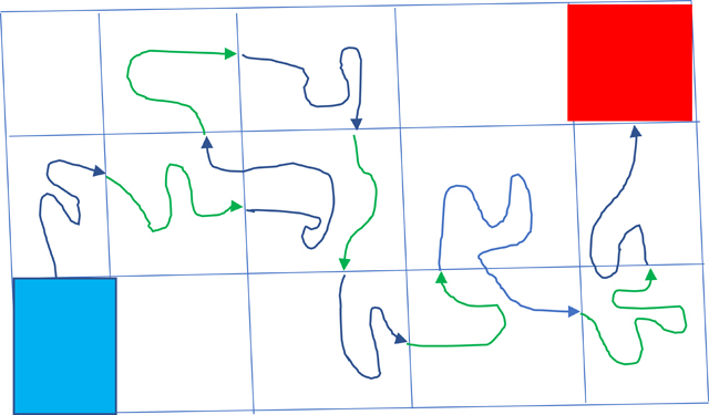
In the last decade, there were significant advances in theories and algorithms to study efficiently long-time dynamics.^2–9 Instead of running complete long trajectories between reactants and products a class of successful approaches use short trajectories.^10–12 The short trajectories are conducted between cells or between cell partitions that cover the reaction space. The short trajectories are analyzed to calculate the overall kinetics and thermodynamics of the system. One of these methods is Milestoning (for a recent review, see¹). The process of running a Milestoning calculation requires multiple steps to establish initial conditions for the trajectories, their termination points, and their statistical weights. It is, therefore, desirable to automate the process as much as possible. Here we present a Python script that organizes and simplifies the job submission of Milestoning. The script, which is called ScMile (Script for Milestoning), currently uses the program NAMD.¹³ Porting the script to other conventional Molecular Dynamics engines is possible and planned for the future.

In the next section, we describe the basic ingredients of the Milestoning algorithm and the requirements from the computing environment. In the third section, we discuss the individual steps and in the fourth section we describe the script. Last, we provide illustrations.

II. The Milestoning Algorithm

We assume that a conventional Molecular Dynamics engine is available (e.g., the program NAMD¹³ that we use here) but that the time of the investigated process is long compared to the simulation time scale. Therefore, it is necessary to use an enhanced sampling approach for kinetics, and it is not practical to use conventional MD.

II.1. Foundations

Consider a system of N particles characterized by a phase space vector $\overrightarrow{x}$ and Hamiltonian $H(\overrightarrow{x}).$ We are interested in long time transitions from reactants to products. The set of all points that are included in a domain R form the reactant state while the points of the domain P are the product state. We seek to model transitions from R to P with particle-based dynamics. We are given equations of motions that can be deterministic or stochastic and can be summarized by a transition matrix or a kernel $K\prime \prime (\overrightarrow{x},t;\overrightarrow{x}\prime ,t^{\prime }),$ which is the probability to arrive to $\overrightarrow{x}$ at time t, given that at time t’ the system was at position $\overrightarrow{x}\prime .$ Given an initial value for the flux (the probability of passing per unit time a phase space point), $\overrightarrow{q}(\overrightarrow{x}(t=0)),$ or the probability of being at $\overrightarrow{x}(t=0),$ $p(\overrightarrow{x}(t=0))$, the kernel is sufficient to generate the fluxes at all times

$$q(\overrightarrow{x}(t))=p(\overrightarrow{x}(t=0))\delta (t)+{\int }_0^t{\int }_{\text{Γ}}q(\overrightarrow{x}\prime (t\prime ))K\prime \prime (\overrightarrow{x}\prime ,t\prime ;\overrightarrow{x},t)d\overrightarrow{x}\prime dt\prime$$ (1)

The integration volume $\text{Γ}$ denotes the whole phase space and $p(\overrightarrow{x}(t=0))$ is the probability of being at $\overrightarrow{x}$ at time zero. The function $\delta (t)$ is the Dirac’s delta function.

Frequently we are concerned with stationary processes in which there is a constant flux of reactants entering the system, and an absorbing boundary is set at the product state, making the total number of transition events time-independent. The stationary process is similar in spirit to the steady-state of chemical kinetics and makes it possible to determine the rate coefficient that can be used in time-dependent processes as well.

To determine the stationary flux, we assume that it exists and consider the limit of $t\to \infty$ of Eq. (1)

$$q_s(\overrightarrow{x})=\underset{t\to \infty }{\lim }\underset{0}{\overset{t}{\int }}dt\prime \underset{\mathrm{\Gamma }}{\int }d\overrightarrow{x}\prime \cdot q_s(\overrightarrow{x}\prime )\cdot K\prime (\overrightarrow{x}\prime ,\overrightarrow{x};\prime t-t\prime )$$ (2)

In Eq. (2) we further assume that the kernel depends only on the time difference $(t-t\prime )$ and not on the absolute value of the time t. We therefore change the notation of the kernel. This setup is typical for systems with a time-independent Hamiltonian. The dependence on the time origin is also inconsistent with stationary processes. Under these conditions, we can define the stationary kernel as

$$K(\overrightarrow{x}\prime ,\overrightarrow{x})\equiv \underset{0}{\overset{\infty }{\int }}dt\cdot K\prime (\overrightarrow{x}\prime ,\overrightarrow{x};t)$$ (3)

Eq. (2) is reduced to

$$q_s(\overrightarrow{x})=\underset{\mathrm{\Gamma }}{\int }d\overrightarrow{x}\prime \cdot q_s(\overrightarrow{x}\prime )\cdot K(\overrightarrow{x}\prime ,\overrightarrow{x})$$ (4)

We think of Eq. (4) as an eigenvector-eigenvalue problem in which the eigenvector to be determined is the flux $q_s(\overrightarrow{x})$ and the eigenvalue is one. Alternatively, we solve Eq. (4) by power iterations

$$q_s^{(n+1)}(\overrightarrow{x})=\int d\overrightarrow{x}\prime q_s^{(n)}(\overrightarrow{x}\prime )\cdot K(\overrightarrow{x}\prime ,\overrightarrow{x})$$ (5)

where the superscripts are the iteration index. The power iterations are converged when $|q_s^{(n+1)}(\overrightarrow{x})-q_s^{(n)}(\overrightarrow{x})|<\epsilon$ where ε is a small positive number. Since the kernel represents transition probabilities, the norms of its complex eigenvalues are smaller or equal to one. Power iterations diminish the contributions of eigenvectors with eigenvalues with a norm less than one. At the limit of a large number of iterations, only the eigenvector with an eigenvalue of one remains. We assume, in accord with experience with physical systems, that there is only one stationary vector.

In Milestoning, we do not consider transitions between all pairs of coordinate vectors. A comprehensive representation of the kernel is formidable and not practical. Instead, we partition the system into cells using “milestones” for cell boundaries.¹ A set of discrete values of the coarse variables determines the milestones. For example, the root-mean-square-distance (RMSD), distances between selected atoms, and torsion angles are examples for coarse variables. The number of coarse variables is much smaller than the number of degrees of freedom of the entire system. Formally, we specify the state of a trajectory by the milestone it crosses last (say α) supplemented by the full coordinate vector of the crossing point in the milestone - $\overrightarrow{x}$. Correspondingly, we write $K_{\beta \alpha }(\overrightarrow{x},{\overrightarrow{x}}^{\prime })$ for the transition probability between milestone $\beta$ at phase space point $\overrightarrow{x}$ and milestone $\alpha$ at phase space point $\overrightarrow{x}\prime .$ The kinetic theory of Milestoning is based on computing transitions between nearby milestones and collecting information about these short-range transitions to build a kinetic model for the entire system. “Nearby milestones” are defined as cell boundaries that can be reached using trajectories that do not cross other milestones in the process.

We write Eq. (5) in the Milestoning language

$$q_{s,\alpha }^{(n+1)}(\overrightarrow{x})=\sum _{\beta }\underset{M_{\beta }}{\int }d\overrightarrow{x}\prime \cdot q_{s,\beta }^{(n)}(\overrightarrow{x}\prime )\cdot K_{\beta \alpha }(\overrightarrow{x}\prime ,\overrightarrow{x})$$ (6)

To solve Eq. (6) by iterations, we need an initial guess for the eigenvector, i.e. $q_{s,\alpha }^{(0)}(\overrightarrow{x})$. We write without loss of generality

$$q_{s,\alpha }(\overrightarrow{x})=w_{\alpha }{f}_{\alpha }(\overrightarrow{x})$$ (7)

where $\underset{M_{\alpha }}{\int }{f}_{\alpha }(\overrightarrow{x})d\overrightarrow{x}=1$ is a normalized probability density of crossing the milestone at different phase space points, and $w_{\alpha }$ is the milestone weight to be determined. $M_{\alpha }$ denotes the domain of milestone α on which the integration is conducted. Substituting Eq. (7) in Eq. (6), integrating over the spaces of the milestones and summing up explicitly the discrete milestones we have

$$\begin{gathered} \underset{M_{\alpha }}{\int }d\overrightarrow{x}\cdot q_{s,\alpha }^{(n+1)}(\overrightarrow{x})=\sum _{\beta }\underset{M_{\alpha }}{\int }\underset{M_{\beta }}{\int }d\overrightarrow{x}\prime d\overrightarrow{x}\cdot q_{s,\beta }^{(n)}(\overrightarrow{x}\prime )K_{\beta \alpha }(\overrightarrow{x}\prime ,\overrightarrow{x}) \\ {w}_{\alpha }^{(n+1)}=\sum _{\beta }{w}_{\beta }^{(n)}\underset{M_{\alpha }}{\int }\underset{M_{\beta }}{\int }d\overrightarrow{x}\prime \cdot d\overrightarrow{x}\cdot f_{\beta }^{(n)}(\overrightarrow{x}\prime )K_{\beta \alpha }(\overrightarrow{x}\prime ,\overrightarrow{x}) \end{gathered}$$ (8)

Let us define

$${\overline{K}}_{\mathit{\beta \alpha }}^{(n)}=\underset{M_{\alpha }}{\int }\underset{M_{\beta }}{\int }d\overrightarrow{x}\prime d\overrightarrow{x}\cdot f_{\beta }^{(n)}(\overrightarrow{x}\prime )K_{\beta \alpha }(\overrightarrow{x}\prime ,\overrightarrow{x})$$ (9)

With the help of the definition in Eq. (9), Eq. (8) takes the simple linear form for the milestone weights:

$$w_{\alpha }^{(n)}\cong \sum _{\beta }{w}_{\beta }^{(n)}{\overline{K}}_{\beta \alpha }^{(n)}$$ (10)

Eq. (10) is a linear equation for the coefficients, $w_{\alpha }^{(n)}$, with a dimension of the number of milestones. We did not use the iteration suggested in Eq. (8) for the milestone weight. A solution is obtained following Eq. (10) for the weight, while iterations apply only on the distribution in the milestone - $f_{\alpha }^{(n)}(\overrightarrow{x})$. One test of convergence is to have $w_{\alpha }^{(n+1)}\cong w_{\alpha }^{(n)}$ in sequential iterations. At the limit of a large n, the weights converge to fixed values.

From a computational perspective, the size of the matrix of Eq. (10), between several hundreds to several thousands, is much smaller than that of the related equation, Eq. (6). Therefore, the solution is obtained by standard linear solvers.

However, the kernel in Eq. (10) is now defined with yet another unknown function - $f_{\beta }(\overrightarrow{x}\prime )$ (Eq. (9)), which is the function that we need to determine by power iteration. We re-write Eq. (8) as

$$\begin{gathered} q_{s,\alpha }^{(n+1)}(\overrightarrow{x})=\sum _{\beta }\underset{M_{\beta }}{\int }d\overrightarrow{x}\prime \cdot q_{s,\beta }^{(n)}(\overrightarrow{x}\prime )K_{\beta \alpha }(\overrightarrow{x}\prime ,\overrightarrow{x}) \\ {w}_{\alpha }^{(n+1)}{f}_{\alpha }^{(n+1)}(\overrightarrow{x})=\sum _{\beta }{w}_{\beta }^{(n)}\underset{M_{\beta }}{\int }d\overrightarrow{x}\prime \cdot f_{\beta }^{(n)}(\overrightarrow{x}\prime )K_{\beta \alpha }(\overrightarrow{x}\prime ,\overrightarrow{x}) \\ {f}_{\alpha }^{(n+1)}(\overrightarrow{x})\cong \frac{1}{w_{\alpha }^{(n)}}\sum _{\beta }{w}_{\beta }^{(n)}\underset{M_{\beta }}{\int }d\overrightarrow{x}\prime \cdot f_{\beta }^{(n)}(\overrightarrow{x}\prime )K_{\beta \alpha }(\overrightarrow{x}\prime ,\overrightarrow{x}) \end{gathered}$$ (11)

Eq. (11) for the distribution function of phase space points in the milestone, $f_{\alpha }^{(n)}(\overrightarrow{x})$, is also linear. However, the distributions are continuous and the iterations in Eq. (11) can be challenging in high dimensions. Note that we approximate $w_{\alpha }^{(n+1)}$ by $w_{\alpha }^{(n)}$ while moving from the second to the third line of Eq. (11). We solve Eq. (11) by power iterations and trajectories. An initial guess for the distribution $f_{\alpha }^{(0)}(\overrightarrow{x})$ is needed for the power iterations. If the system is near equilibrium it is suggestive to try:

$$f_{\alpha }^{(0)}(\overrightarrow{x})=\frac{\exp (-\beta U({\overrightarrow{x}}_{\alpha }))}{Z_{\alpha }}$$ (12)

The potential energy is denoted by $U(\overrightarrow{x})$, β is the Boltzmann factor, and the notation ${\overrightarrow{x}}_{\alpha }$ is to indicate that the coordinate vector is conditioned to be at milestone α. The normalization Z_α is given by $Z_{\alpha }=\underset{M_{\alpha }}{\int }d{\overrightarrow{x}}_{\alpha }\cdot \exp \left[-\beta U({\overrightarrow{x}}_{\alpha })\right].$

Another function that we compute is the milestone lifetime, $t_{\alpha }({\overrightarrow{x}}_{\alpha }).$ It is the average time for a trajectory initiated at milestone α and position ${\overrightarrow{x}}_{\alpha }$ on the milestone to hit any other milestone. We also define, $t_{\alpha },$ which is averaged over the initial conditions at the milestone

$$\begin{gathered} t_{\alpha }(\overrightarrow{x})=\sum _{\beta }\underset{M_{\beta }}{\int }d\overrightarrow{x}\prime \cdot t(\overrightarrow{x})\cdot K_{\alpha \beta }(\overrightarrow{x},\overrightarrow{x}\prime ) \\ {t}_{\alpha }=\underset{M_{\alpha }}{\int }d\overrightarrow{x}\cdot f_{\alpha }(\overrightarrow{x})t_{\alpha }(\overrightarrow{x}) \end{gathered}$$ (13)

The main results of this section are Eq. (10), (11) and (13). In the next section, we describe how they can be solved by sampling trajectories.

II.2. Trajectory sampling in Milestoning

In this section we are concerned with trajectory sampling of the distributions $f_{\alpha }^{(n)}(\overrightarrow{x})\forall \alpha$ and solving Eq. (11). Consider Eq. (12) for the initial guess for the distribution $f_{\alpha }^{(0)}(\overrightarrow{x}).$ From this known distribution we sample $n_{\alpha }$ initial conditions, ${\left\{{\overrightarrow{x}}_i\right\}}_{i=1}^{n_{\alpha }},$ using Molecular Dynamics at a constant temperature, ${\beta }^{-1},$ constrained to the hypersurface of the α milestone. These initial conditions for the trajectories,

$$f_{\alpha }^{(0)}(\overrightarrow{x})=\frac{1}{n_{\alpha }^{(0)}}\sum _i\delta ({\overrightarrow{x}}_i-\overrightarrow{x})$$ (14)

are now placed in Eq. (9) to determine the average kernel

$${\overline{K}}_{\beta \alpha }^{(1)}=\underset{M_{\alpha }}{\int }\underset{M_{\beta }}{\int }d\overrightarrow{x}\prime \cdot d\overrightarrow{x}\cdot \left(\frac{1}{n_{\beta }^{(0)}}\sum _i\delta ({\overrightarrow{x}}_i-\overrightarrow{x}\prime )\right)K_{\beta \alpha }^{(0)}(\overrightarrow{x}\prime ,\overrightarrow{x})=\frac{n_{\beta \alpha }^{(1)}}{n_{\beta }^{(0)}}$$ (15)

The number of trajectories, $n_{\beta }$ should be sufficiently large to allow accurate estimates of the elements of the transition kernel. Once the initial conditions are given, the kernel that determines the dynamics propagates the individual trajectories until they hit for the first time another milestone α. The milestones are placed such that the trajectories are short and can be computed efficiently by a conventional MD engine. The number of trajectories that were initiated at milestone β and terminated at milestone α is $n_{\beta \alpha }^{(1)}.$ Once the averaged kernel is determined we may continue to Eq. (10), solve the linear equations, and determine the unknown milestone weights $w_{\alpha }^{(1)}.$

$$w_{\alpha }^{(1)}=\sum _{\beta }{w}_{\beta }^{(1)}\cdot \left(\frac{n_{\beta \alpha }^{(1)}}{n_{\beta }^{(0)}}\right)$$ (16)

With the weights of the milestones at hand, we can continue to Eq. (11) and determine the new distribution of phase space points in the hypersurface of the milestone.

$$f_{\alpha }^{(1)}(\overrightarrow{x})=\frac{1}{w_{\alpha }^{(1)}}\sum _{\beta }{w}_{\beta }^{(1)}\underset{M_{\beta }}{\int }d\overrightarrow{x}\prime \cdot \frac{1}{n_{\beta }^{(0)}}\sum _i\delta ({\overrightarrow{x}}_i-\overrightarrow{x}\prime )\cdot K_{\beta \alpha }(\overrightarrow{x}\prime ,\overrightarrow{x})$$ (17)

Convergence of the iterations can be assumed if $|w_{\alpha }^{(n)}-w_{\alpha }^{(n+1)}|<\epsilon$ and $|f_{\alpha }^{(n+1)}(\overrightarrow{x})-f_{\alpha }^{(n)}(\overrightarrow{x})|<\epsilon$. Since the initial conditions of the trajectories are presented by a sum over Dirac’s delta functions, their continuous distribution is hard to converge and test. Instead, we examine the convergence of observables such as the free energy and the mean first passage time (see section II.3).

The calculation of the lifetimes of the milestones (Eq. (13)) with trajectories is straightforward

$$t_{\alpha }=\frac{1}{n_{\alpha }}\sum _{i=1,\mathrm{...},n_{\alpha }}{t}_i$$ (18)

We sum over the termination times of individual trajectories initiated at milestone α. A termination time, $t_i,$ is the first time a trajectory hits a milestone different from α.

In the next section, we briefly describe how the flux can be used to compute other observables of interest.

II.3. Observables

Once sets of trajectories between milestones are sampled, many observables can be computed. We focus here, however, on three main outcomes: the free energy profile, the Mean First Passage Time, and the committor function. Calculations of observables were derived and discussed extensively elsewhere.¹¹ Here we briefly quote the main results that are based on the calculations of the flux and the lifetime of the milestones mentioned in an earlier section.

The last milestone that a trajectory crosses (say α), defines the state of the trajectory. Since a milestone is a divider between two cells, the trajectory of milestone α can be found in any of the two cells that are partitioned by the α milestone. Since the time of crossing a milestone can be measured or computed precisely, the Milestoning theory is exact provided that the lower spatial resolution of the trajectories is acceptable. This is different (for example) from the Markov State Model,¹⁴ which assigned a trajectory to a cell (and a finite volume) for which the time of entrance and exit can be determined only up to a local “incubation” time in the cell.

The free energy of a milestone is given by Eq. (19)¹⁵ where we impose reflecting boundary conditions on the reactant and product states to make an equilibrium state possible

$$F_{\alpha }=-k_{B}T\log \left[p_{\alpha }\right]=-k_{B}T\log \left[\underset{M_{\alpha }}{\int }d\overrightarrow{x}\cdot q_{\alpha }(\overrightarrow{x})\cdot t_{\alpha }(\overrightarrow{x})\right]=-k_{B}T\log \left[w_{\alpha }\cdot t_{\alpha }\right]$$ (19)

The overall Mean First Passage Time (MFPT) at a steady-state condition (in which probability is absorbed at the product state and the reactant state is injected with new probability at a constant balancing rate) is given by the following two closely-related expressions¹¹

$$\langle \tau \rangle =\frac{\sum _{\alpha }\underset{M_{\alpha }}{\int }d\overrightarrow{x}\cdot q_{\alpha }(\overrightarrow{x})\cdot t_{\alpha }(\overrightarrow{x})}{\underset{M_f}{\int }d\overrightarrow{x}\cdot q_f(\overrightarrow{x})}$$ (20.a)

$$\langle \tau \rangle =\mathbf{p}(0){(\mathbf{I}-\mathbf{K})}^{\mathbf{-}1}\mathbf{t}$$ (20.b)

One interpretation of Eq. (20.a) is of population over the outgoing flux out $(p/q_f)$ which is a well-known expression for the MFPT, see for instance.¹⁶ We have shown that the probability of being at state $\alpha$, $p_{\alpha }(\overrightarrow{x})$, is given by the flux into that state $q_{\alpha }(\overrightarrow{x})$ multiplied by the life time of that state, $t_{\alpha }(\overrightarrow{x})$. The summation over all states in Eq. (20.a) brings the probability. The summation over the outgoing flux is conducted in the denominator.

An alternative and related formula for the MFPT is given in (20.b) in a matrix-vector notation. It is discussed extensively in references ^{11, 17} and its relationship to the expression in (20.a) is derived. The vector $\mathbf{p}(0)$ is the probability at the reactants at stationary conditions, $\mathbf{I}$ is the identity matrix, $\mathbf{K}$ the kernel matrix, and $\mathbf{t}$ the vector with the milestone lifetimes. We typically are using both formulae as a check.

The committor function, $C_{\alpha }$,¹⁸ is the probability that trajectories starting from milestone $\alpha$ will reach for the first time the product before the reactant. It can be computed from the compact linear equation.

$$C_{\alpha }(\overrightarrow{x})=\sum _{\beta }\underset{M_{\beta }}{\int }d\overrightarrow{x}\text{'}\cdot K_{\alpha \beta }(\overrightarrow{x},\overrightarrow{x}\text{'})C_{\beta }(\overrightarrow{x}\text{'})$$ (21)

The following boundary conditions are implemented into the kernel: The trajectories that enter the product state are trapped, while the trajectories that enter the reactant state disappear. In addition, we impose boundary conditions on the committor: $C_R=0$ and $C_P=1$ where C_R and C_P are the committor values at the reactant and product respectively. The last conditions make Eq. (21) an inhomogeneous linear equation with a well-defined solution. Since the committor function is used for qualitative analysis of the dynamics, we are frequently satisfied with an approximation, which is equivalent to doing only a single iteration of Milestoning. Eq. (22) for the committor as a function of the milestone indices is

$$C_{\alpha }=\sum _{\beta }{\overline{K}}_{\alpha \beta }{C}_{\beta }$$ (22)

with the same boundary conditions as discussed above for the exact expression.

II.4. Representation of the milestones

The milestones are dividers between cells in reaction space. The reaction space is determined by several coarse variables, such as root mean square distance, torsion angles, or even by a single reaction coordinate. The number of coarse variables is always much smaller than the number of degrees of freedom in the system. Nevertheless, the coarse variables are expected to capture the progress of the reaction. We denote the set of coarse variables by the vector $\overrightarrow{Q}.$ Frequently, we are using cells and milestones that are defined by Voronoi cells. The use of milestones as the boundaries separating Voronoi cells is a clever advance suggested by Vanden Eijnden.¹⁹ Sampled configurations between reactants and products determine the centers of Voronoi cells, ${\left\{{\overrightarrow{Q}}_j\right\}}_{j=1}^J.$ In Milestoning, we call these configurations “anchors”.²⁰ The sampled configurations may be along a one-dimensional reaction coordinate that is assumed,¹⁵ or computed in advance.²¹ A configuration, $\overrightarrow{Q}$, belongs to cell $i$ if the distance $|\overrightarrow{Q}-{\overrightarrow{Q}}_i|$ is smaller than all other distances $|\overrightarrow{Q}-{\overrightarrow{Q}}_j|\forall j\ne i$. The configurations $\overrightarrow{Q}$ belongs to milestone $M_{\alpha }$ that separates cells $i$ and $j$ if

$$|\overrightarrow{Q}-{\overrightarrow{Q}}_i|=|\overrightarrow{Q}-{\overrightarrow{Q}}_j|<|\overrightarrow{Q}-{\overrightarrow{Q}}_k|\forall k\ne i,j$$ (23)

III. The Milestoning Algorithm in Steps

A Milestoning simulation is split into the following steps:

• 1Define the coarse variables and anchors (user input)

The identification of a small number of coarse variables that best describes the reaction is a topic that is investigated intensely. There are several promising approaches in the field, such as the diffusion maps.²² However, the use of chemical and physical intuition is a still very common. In the current version of ScMiles we require the user to define the coarse variables. The coarse variables are determined and used through the program COLVAR.²³ We also require COLVAR to determine the anchors in the space of coarse variables. The anchors are typically obtained from a previous exploratory simulation of the process²⁴ or reaction path calculations.²⁵

• 2Identifying milestones (exploratory and automated Milestoning simulations)

If the number of anchors is $N_A$ the maximum number of milestones possible is $N_A(N_A-1)/2.$ If a typical number of anchors is between one hundred to one thousand, the maximal number of milestones is between ten thousand and a million. The simulation requires that at each milestone we sample and launch about 100 unbiased trajectories. The computational cost of conducting up to 100 million trajectories, even if they are of only a few picoseconds, is overwhelming.

However, not all possible milestones are accessible or essential. For a one-dimensional reaction coordinate, the number of milestones is only $N_A-1$ In higher dimensions, the number of milestones can be higher, but it still quite far from the maximum. To keep the calculations efficient, we first search for the most important milestones. We use a function called seek, following the original script of Majek.²⁰ We conduct ~50–100 unbiased trajectories with different initial velocities, starting from each of the anchors. The trajectories are conducted until they hit for the first time a milestone between the initial and another anchor (such that the condition of Eq. (23) is satisfied). The last configuration of the trajectory “touching” the newly discovered boundary between the two anchors activates the milestone, which is added to a list. It also provides an initial configuration for sampling at the milestone, which is discussed next. The seek approach, as described, is not necessarily comprehensive. However, it was found satisfactory in many studies.^1,9,15,20

• 3Sampling configurations at each milestone (automated Milestoning simulation)

The previous step provides atomically detailed configurations $\overrightarrow{x}(t)$ such that $\overrightarrow{Q}(\overrightarrow{x}(t))$ are at milestones. In this step, we sample configurations at the “marked” milestones. We conduct constant temperature Molecular Dynamics simulations conditioned to remain at the milestones. The conditions or constraints are implemented with COLVAR, which is interfaced to NAMD. We add harmonic potentials to the simulation energy

$$V_{ij}=k{(|\overrightarrow{Q}(t)-{\overrightarrow{Q}}_i|-|\overrightarrow{Q}(t)-{\overrightarrow{Q}}_j|)}^2$$ (24)

The coefficient $k$ is the restraint force constant. We also add half harmonic restraint to ensure that the trajectory $k$ anchors $k\ne i,j$

$$\begin{gathered} V_{ik}=\left(\begin{array}{cc}k(|\overrightarrow{Q}(t)-{\overrightarrow{Q}}_k|-{|\overrightarrow{Q}(t)-{\overrightarrow{Q}}_i|}^2)& \text{if }|\overrightarrow{Q}(t)-{\overrightarrow{Q}}_i|>|\overrightarrow{Q}(t)-{\overrightarrow{Q}}_k|\\ 0& \text{otherwise}\end{array}\right) \\ {V}_{jk}=\left(\begin{array}{cc}k(|\overrightarrow{Q}(t)-{\overrightarrow{Q}}_k|-{|\overrightarrow{Q}(t)-{\overrightarrow{Q}}_j|}^2)& \text{if }|\overrightarrow{Q}(t)-{\overrightarrow{Q}}_j|>|\overrightarrow{Q}(t)-{\overrightarrow{Q}}_k|\\ 0& \text{otherwise}\end{array}\right) \end{gathered}$$ (25)

The set of full configurations, $\overrightarrow{x}(t)$, that we obtained from the sampling at each of the milestones are used in the next step.

• 4Conducting unbiased trajectories

From the configurations sampled at the milestones and kept for further calculations in step (3) we launch unbiased trajectories. Typically, the number of trajectories that we launched from each milestone is 100. The input is set to run for a fixed length of time which is longer than a typical termination time at the milestones. During the run, COLVAR, which is interfaced to NAMD, detects the crossing events and terminates the trajectories at the times of crossing. The first time in which the launched trajectory crosses a new milestone (different from the milestone it was initiated on), the identity of the crossed milestones, the coordinates, and the time of the crossing are recorded.

• 5Analyzing the results

From step 4 we obtained a sample of crossing events that we use to estimate functions of the Milestoning theory. We are ready to estimate the kernel from the trajectories

$${\overline{K}}_{\alpha \beta }=\frac{1}{n_{\alpha }}\sum _l{\delta }_{l,\alpha \to \beta }=\frac{n_{\alpha \beta }}{n_{\alpha }}$$ (26)

The ${\delta }_{l,\alpha \to \beta }$ is a Kronecker delta function. It is one if the trajectory $l$ that is initiated in milestone $\alpha$ hits for the first-time milestone $\beta$. It is zero if a milestone different from $\beta$ (and $\alpha$) is hit. The kernel is, therefore, an average of a stochastic variable that accepts the values of zero or one. The distribution of the kernel elements is known and discussed in the supplementary material of reference.²⁶ It is the so-called $\beta$ distribution

$$P({\overline{K}}_{\alpha \beta })=\frac{\mathrm{\Gamma }(n_{\alpha })}{\mathrm{\Gamma }(n_{\alpha \beta })\mathrm{\Gamma }(n_{\alpha }-n_{\alpha \beta })}{\overline{K}}_{\alpha \beta }^{(n_{\alpha \beta }-1)}{(1-{\overline{K}}_{\alpha \beta })}^{(n_{\alpha }-n_{\alpha \beta }-1)}$$ (27)

The distribution of $t_{\alpha }$ (Eq. 18) which is an average of termination times of individual trajectories should follow central limit theorem and is assumed normal. To estimate the statistical errors of the observables, we repeat their calculations using sampled kernels and lifetimes from their known distributions. We use a sample size of one thousand to compute the observables and their variances.

• 6Convergence check and preparation for next iteration

Given a force field and a reasonable selection of coarse variables that differentiate between reactants and products there are two sources of errors in Milestoning. The first is a statistical error, namely the effective sampling of transitions between milestones in a single iteration. The second is the convergence of the distribution in the milestone - $f_{\alpha }^{(n)}(\overrightarrow{x})$ as a function of the iteration index n.

As a first check, we examine the statistical errors of the main observables: free energy and MFPT, using an ensemble of transition matrices (Eq. (27)), and lifetimes. If the errors are larger than expected, we probe in more details the source of the errors. For example, two neighboring milestones may be separated by a significant free energy barrier, and none or only a few transitional trajectories are sampled between the two milestones. In that case, the errors of the corresponding element of the kernel will be large. The solution is to run more trajectories initiated at the offending milestone. Alternatively, we may add an anchor (and two milestones) between two milestones that are difficult to connect. The corrections mean that we either return to step 3 (to run more trajectories) or to step 2 if we add milestones.

Another source of errors is the deviation of $f_{\alpha }^{(n)}(\overrightarrow{x})$ from the stationary distribution, $f_{\alpha }^{(\infty )}(\overrightarrow{x})$. It is difficult to compare the distributions directly since the sample in the large space of the individual milestones is sparse. Therefore, we check the observables such as the free energy and the MFPT for convergence as a function of the iteration number. To run the next iteration, we use the termination points of the trajectories initiated according to the distribution $f_{\alpha }^{(n)}(\overrightarrow{x})$ to obtain an estimate for $f_{\alpha }^{(n+1)}(\overrightarrow{x}).$¹¹ Once the distribution $f_{\alpha }^{(n+1)}(\overrightarrow{x})$ is at hand we return to step 4 and conduct unbiased trajectories.

The distributions generated from termination points of trajectories are not necessarily sampled evenly. Some milestones may capture only a small number of terminating trajectories, generating poor statistics for the next iteration. Two approaches may improve the poor statistics: First, we may define a mixture of distributions at the milestone that include previous and current distributions. For example, $f_{\alpha }^{(n+1)\prime }=\lambda f_{\alpha }^{(n+1)}+(1-\lambda )f_{\alpha }^{(n)}$ where $\lambda \in \left[0,1\right]$ is a mixing parameter, and sample from the mixture. The retention of the previous iterations ensures that the sampling is adequate even if the rate of convergence is slower. Second, more phase space points can be generated at the milestone by sampling new velocities from the Maxwell distribution using the same terminating coordinates and running Newtonian trajectories. This choice is similar to Weighted Ensemble splitting of trajectories which is based on the same coordinate but an application of a stochastic force.⁴ In the present manuscript, we enrich the distributions at the milestone only with the second approach of reassignments of velocities.

IV. The Milestoning Script (ScMiles)

A Milestoning simulation using the newly written Python script, ScMiles, (Script for Milestoning) is exploiting several software packages. First, it uses the Python 3 version of the scripting language (with Anaconda3 recommended). Second, it uses the software package NAMD¹³ to run individual trajectories. Third, it is using COLVAR²³ to imposed the Milestoning constraints. Fourth, the job schedulers PBS or Slurm are used to manage the submission of multiple trajectories on a computer cluster. It is planned to extend the applicability of ScMiles to other Molecular Dynamics engines and submission management tools, but the current release is restricted to the above options. ScMiles is available from https://github.com/UTweiw/ScMiles, earlier variants of Milestoning scripts were written by Majek,²⁰ and more recently by Bello https://github.com/jmbr/miles for exact Milestoning. We describe below the operation of the software.

Once the ScMiles.zip is downloaded from the depository it is convenient to create a directory and open the zip files in a separate directory. Two folders will be created: ScMiles and my_project_input.

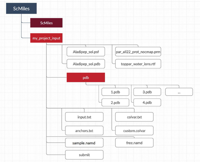
A flow chart of the organization of the Milestoning data is shown in Fig. 1. In the discussion of the software below, we reference section III in which the algorithm is explained in more details. These references help establish the connection between the theory, algorithm and its implementation.

Fig. 1.

A flow chart of the organization of Milestoning data.

The subdirectory ScMiles includes the Python source code and normally should not be modified by the user. The directory my_project_input stores the necessary input for Milestoning calculations. The first set of files in my_project_input (Aladipep_sol.psf, Aladipep_sol.pdb, par_all22_prot_nocamp.prm, and toppar_water_ions.rtf) are NAMD data files for energy evaluations. The second set of files stored in the subdirectory pdb are the coordinate sets of the anchors labelled as (1.pdb 2.pdb …). The files include the complete coordinate vectors that are necessary to conduct atomically detailed simulations.

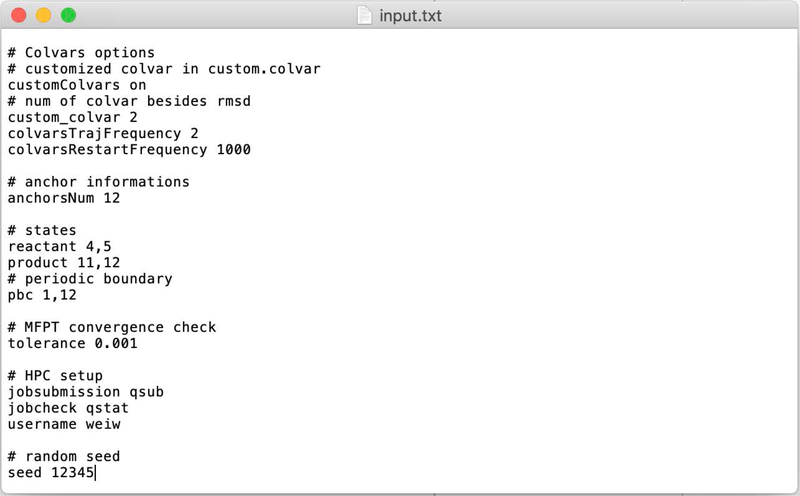
The first file from the top-to-down view that is directly connected to Milestoning is the file input.txt that we discuss below.

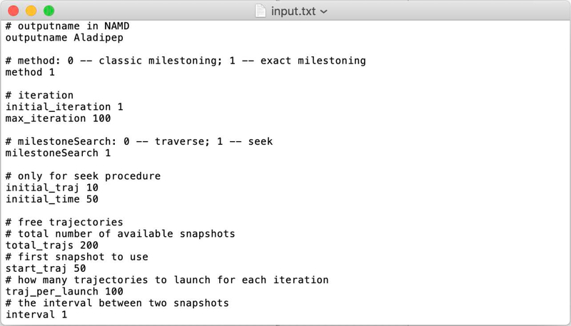
A sample input.txt is given in Fig. 2

Fig. 2.

A sample input file for ScMiles.

In the input file comment lines start with #. The outputname line provides an identifier for NAMD output.

The “method” line chooses between a Milestoning calculation of a single iteration (so-called classical Milestoning), and exact Milestoning (Milestoning with multiple iterations). Here “exact Milestoning” is chosen. The next command line selects the maximal number of iterations in exact Milestoning. The computations can finish earlier if the obseravbles converge numerically in a smaller number of steps. Here max_iteration is equal to 100.

The expression milestoneSearch is used at the beginning of the calculations to determine the location of the milestones from the pre-determined positions of the anchors (it is step 2 of section III). One possibility (traverse) is to assume a one-dimensional reaction coordinate. In that case, the script is placing the milestones between sequential anchors. A milestone position is determined by averaging the coarse variables of the anchors sandwiching that milestone.

In the second option (seek), trajectories are initiated from the anchors and are terminated when they hit another milestone for the first time. I.e., the trajectory is stopped and the identities of the anchors are recorded at the first time a trajectory configuration has the same distance from the new and initiating anchors. The newly determined values of the coarse variables between the two anchors define the milestone.

For the “seek” option, we provide the number of trajectories initiated from each anchor (initial_traj). In the example, the number of trajectories is 10, a more typical value in complex systems is 100. The variable “initial_time” determines the maximum length of the “seek” trajectories, which here is set to 50 picoseconds. Since the anchors are close, we do not expect “seek” trajectories to be long. The seek time is determined in practice by the density of milestones, but 50 picoseconds for a seek time is typical.

The next few command lines set the parameters for the trajectories. In the first iteration, there are two types of trajectories that we use: (i) Sampling in the milestone according to Eq. (12) (step 3 in section III) and (ii) conducting trajectories between milestones (step 4 of section III). In the second and higher order iterations we only use trajectories of type (ii) since the termination events provide the sampling in the milestone for the next iteration.

The number of trajectories of type (i) is given by the command line “total_trajs 200”, which is the number of saved sampling points in the milestone. We are using the “restart” option of NAMD¹³ to save configurations and velocities for trajectory initiation. The restart option is important for exact Milestoning in which the velocities are needed to continue the trajectories exactly. The rate of saving configurations is determined by the input to the Molecular Dynamics program. From the 200 structures that we save, we skip some structures at the beginning (50) to enable relaxation at the milestone.

The command “traj_per_launch 100” determines how many unbiased trajectories between milestones to launch. In the above example, we generate 200 sampled points. We skipped the first 50 trajectories and then generated 100 trajectories, which is a typical number. In the example, we have in reserve 50 more sample points to initiate trajectories, in case that they are needed.

Finally, “interval” is the spacing between the configurations that we use. For example, “interval 10” is an indicator to use structures 51, 61, 71... and so on from the set of 200 structures that we prepared (skipping the first 50). This option is useful to test for, and potentially reduce, correlation between the trajectories.

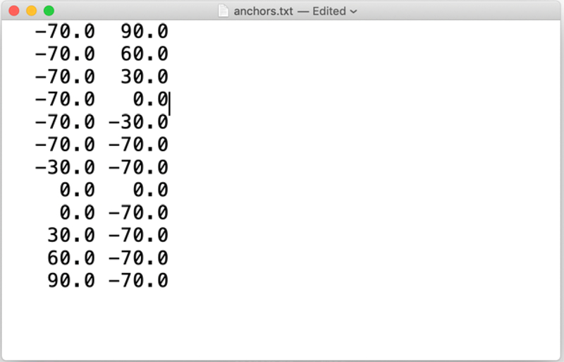
We provide complete coordinate sets for the anchors in the subdirectory “pdb” (step 1 of section III). However, it is convenient to provide the anchor definitions in terms of the values of their coarse variables. This list is provided in the file “anchor.txt”. Every line in the file lists all the values of the coarse variables for an anchor. The example in Fig. 3 has two coarse variables per anchor.

Fig. 3.

The file anchor.txt provides the values of the coarse variables for each of the twelve anchors.

In a Milestoning run we exploit the coarse variables in two ways. First, the coarse variables are used to generate constrained samples at the milestones. Second, crossing events of milestones by unbiased trajectories are determined according to the value of the coarse variables as a function of time. Therefore, efficient and accurate evaluations of coarse variables is important. We use the program COLVAR for manipulations of coarse variables.²³ The file input.txt includes specific instructions how to communicate with COLVAR (step 1 of section III).

The parameter customColvars can be turned on or off. It is turned on if we wish to track a set of coarse variables as a function of time during the trajectories and print them to the file colvar.traj. By default, a coarse variable is the distance (RMSD) between structures. The user can introduce more coarse variables. Here existence of two new coarse variables is declared (custom_colvar 2). The parameters colvarTrajFrequency is the frequency in which the coarse variables are saved in the memory. The colvarsRestartFrequency is the frequency in which the coarse variables are written into the colvar.traj hard-disk file.

The rest of the parameters are not about COLVAR. The line of anchorNum determines the number of anchors. The reactant and product states are determined by two bounding milestones in one dimension (e.g. reactant 4,5). Alternatively, a single number can be given which is understood to be an anchor. In the option of one-dimensional Milestoning, the milestones are determined by the sequence of the anchors. Therefore, the periodic boundary condition is set explicitly by two anchors. The script adds a milestone between the two anchors, here they are 1 and 12 (pbc 1, 12).

We are using the MFPT as a test of convergence of the exact Milestoning calculation (tolerance 0.001). In the above example if the relative error is less than 0.1% the iterations stop even before the limit of max_iteration.

The final parameters are required for job submission (jobsubmission, jobcheck, and username).

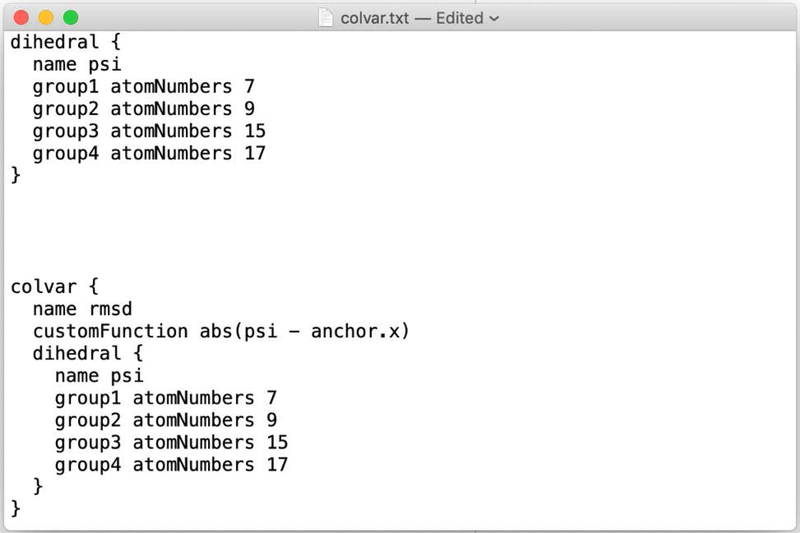
A sample input for COLVAR (colvar.txt) as used in Milestoning is given below.

Note that the “rmsd” is the distance in coarse space typically between the current configuration and an anchor (see also Eq. (25)).

The files (i) sample.namd and (ii) free.namd are standard NAMD files that are used (respectively) to (i) sample configurations in the milestones using constrained trajectories, or to (ii) launch unbiased trajectories from the milestones initiated from existing samples. A few comments: All the parameter files must use absolute paths. A restart file must be saved frequently in the “sample” runs since they are used as initial conditions for unbiased trajectories. More information can be found in the depository, including submission files for the PBS and Slurm systems.

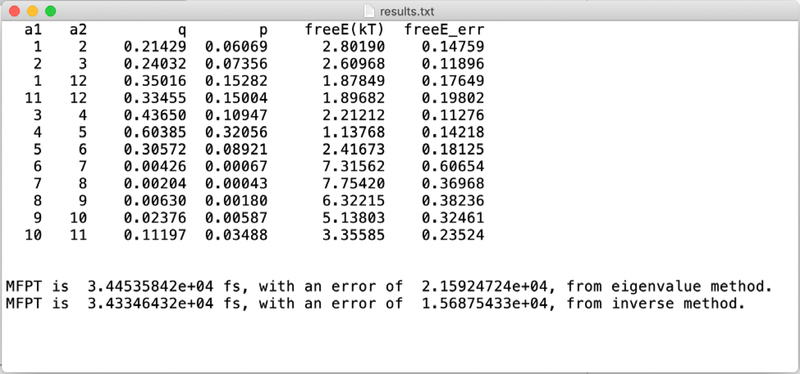
The output of the Milestoning are stored in the directory my_project_output, which is found under the main head of ScMiles (step 5 and 6 of section III). The file results.txt in that directory summarizes the main results (Fig. 6).

Fig. 6.

A summary of the results of a Milestoning run. The columns labeled “a1” and “a2” denote the two anchors that define a milestone. A milestone in the script is defined by the two anchors that “sandwich” it. The stationary flux is found in the column “q”. The probability of last crossing the row milestone is “p”. The free energy of the milestone in unit of kT is “freeE(kT)”. An error estimate for the free energy value is “freeE_err”. The last two lines list the MFPT values and error estimates. Two estimates are given using the expressions in Eq. (20.a) and (20.b), respectively. The results should be the same, but sometimes numerical errors are encountered and it is useful to have the two values as a “sanity” check. The additional computational efforts are negligible.

Detailed information about the trajectory counts that produces the kernel $\mathbf{K}$ is provided in the file k.txt (Fig. 7)

Fig. 7.

Counting of transitions between milestones to estimate the kernel elements. The data are an MxM matrix where M is the number of milestones. The columns are labeled by the two anchors that form a milestone. The same order of milestones is assumed for the rows. For example, 89 of the 100 trajectories initiated at milestone 6_7 reach milestone 5_6, and 11 reached milestone 7_8. Note that all the trajectories initiated at a milestone must terminate. The sum of the counts over a row is, therefore, equal to the total number of trajectories initiated at that milestone.

Information about the lifetimes and committor values of the milestones is found in life_time.txt and committor.txt. Coordinate sets sampled during the trajectories are stored in the subdirectory crd, which is just below the main ScMiles directory. The directory crd is divided between milestones. For example, the directory crd/1_2 include coordinate sets associated with the milestone 1_2. The subdirectories crd/1_2/1, crd/1_2/2 … includes the coordinate for iteration 1 and iteration 2 of exact Milestoning. The file crd/1_2/½0 contains the trajectory number 20 initiated at milestone 1_2 in the first (1) iteration. Another subdirectory crd/1_2/restarts includes the restart files that are used to initiate unbiased trajectories from milestone 1_2 in the next iteration of exact Milestoning.

Another feature that is used in exact Milestoning is of trajectory enrichment (section III point 6). If the number of trajectories that reach a particular milestone is low, we enrich the number of trajectories for the next iteration. For example, if the goal is to run 100 trajectories from each milestone and only 20 terminate at a milestone after an exact Milestoning iteration, we use each of the 20 termination points five times by re-assigning random velocities to these configurations. Records of these enrichments are found under each iteration directory in the files: distribution and enhanced.

V. Examples

We provide two examples of studies of conformational transitions in alanine dipeptide: (1) in a vacuum, and (2) in a solvent. Alanine dipeptide is a frequent test system for new algorithm in molecular dynamics. In the calculations we compare the Milestoning results to a long trajectory using conventional MD. Each of these studies present different challenges for the algorithm and its comparison to straightforward MD.

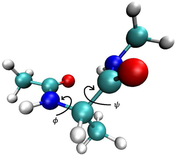
The system in vacuum includes only a small number of degrees of freedom (22 particles, but only two main flexible torsions - $(\varphi ,\psi )$ see Fig. 8). Nevertheless, this small system still presents several challenges. First, it is hard to describe the reaction path with a single reaction coordinate and therefore the anchors and milestones are placed in at least two dimensions. Second, the small number of degrees of freedom makes it difficult to reach ergodicity. We therefore use Langevin dynamics (with a friction coefficient of 5 ps⁻¹) to ensure that conventional MD trajectories are ergodic. Third, there is a significant barrier (of about 8 kcal/mol) separating the two conformations we investigate. This barrier makes it difficult to sample transitions in straightforward MD simulations. To be able to compare Milestoning and conventional MD we conducted the straightforward MD simulations and the Milestoning calculations in vacuum at 600 K. This ensures that in microsecond simulations we sampled enough transitions to estimate the MFPT.

Fig. 8.

A stick and ball model of alanine dipeptide. Also shown are the dihedral angles $(\varphi ,\psi )$ that are the coarse variables used in the present study.

In the second example, of alanine dipeptide solvated in water, a single coarse variable is sufficient to describe the kinetic and the thermodynamics of the system (the ψ dihedral angle, Fig. 8). On the other hand, the inclusion of explicit solvent, adds noise and sampling complexity to the conformational transition compared to the vacuum case. The two examples, therefore, explore different characteristics of the Milestoning algorithm.

V.1. Alanine dipeptide in vacuum.

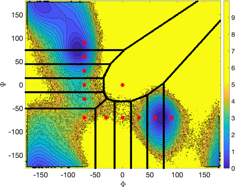
The alanine dipeptide is represented by a vector $\overrightarrow{x}$ that includes the coordinates of all the atoms in the system. The space of coarse variable is effectively two dimensional and consists of the two dihedral angles ϕ and ψ The structure of alanine dipeptide illustrating the dihedral angles is shown in Fig. 8. The CHARMM22 force field²⁷ is used with a cutoff distance of 10 Å. Time step is 1 femtosecond (fs), and the SHAKE algorithm is used to constrain all bond lengths.²⁸ Twelve anchors are placed as shown in the ϕ and ψ map of Fig 9, roughly following the location of the minima and the pathway that connects them at the center of the map. Half harmonic walls are placed at +/− 175 degrees for both ϕ and ψ boundaries with force constants of 1 kcal/mol $\times {\mathrm{degree}}^{-2}$ in order to prevent transition through the map edges. That is, we focus on transitions that pass through the center of the map of Fig. 9.

Fig. 9.

Milestoning and anchors for alanine dipeptide in vacuum. The anchors are denoted by red dots and the milestones by a solid line. The anchor at the lower right corner represents the product while the anchor at the top left corner, the reactant. We also show a color contour map generated by binning configurations extracted from a 2 $\mu s$ straightforward Langevin trajectory.

In Fig. 9 we show a $(\varphi ,\psi )$ free energy map for alanine dipeptide, indicating the location of the anchors by red circles and the milestones by solid lines. The anchor at the top left corner marks the “reactant” and the anchor at the bottom right, the “product”. The milestones between the anchors are computed according to the definition in Eq. (23). Note that the anchors are determined in coarse space while the trajectories (biased or unbiased) are conducted in the full $\overrightarrow{x}$ space. We also show a counter plot of the free energy which is extracted from a long and straightforward MD simulations of $2\mu s$ length. The scale of the energy landscape (in kcal/mol) is indicated on the color bar on the right-hand side of the figure.

While the anchors were placed on the energy landscape rather arbitrarily, the milestones were determined by computations. Since the number of milestones can be very large, especially in high dimensions of coarse variables, and since not all of them are significant for the progress of the reaction, we sample milestones with the “seek” command instead of enumerating them exhaustively. We use the “seek” option in which trajectories are initiated from the anchor and simulated until they hit a milestone. We conducted 100 unbiased trajectories from each of the anchors. For each anchor the trajectories are initiated from the same configuration but with different velocities sampled from the Maxwell distribution at a temperature of 600 K.

Using the trajectory termination points we initiated sampling runs constrained to the milestones to estimate $f_{\alpha }^{(0)}(\overrightarrow{x})$ (section III, step 3) at 600K. The lengths of the constrained simulations were 700 picoseconds (ps) at each of the milestones. The first segment of 200 picoseconds is considered a pre-equilibration run and is ignored. Structures were saved every 1 ps of the remaining 500 ps trajectory. Five hundred phase space points of the sampled structures at each of the milestones initiate unbiased trajectories (step 4 in section III).

Once the first iteration was completed, we continue to conduct additional iterations. Because the sampling at some milestones is poor, we add initial phase space points at these milestones. On the average, we add 250 phase space points by using existing coordinate vectors and re-sampling velocities from the Maxwell distribution (section III, step 6). As the iterations progress, we checked for convergence (step 5, section III).

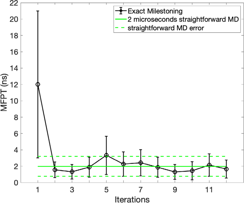
In Fig 10 we show the value of the MFPT as a function of the iteration number. The error bars are statistical and are estimated from a sample of kernels and lifetimes (section III, step 6). The MFPT at 600K is about 2 nanoseconds. The value is essentially converged after two exact Milestoning iterations. Follow up iterations fluctuate around the average value. The fluctuations are caused by limited sampling and need for enrichment on some milestones. Overall the agreement between straightforward simulations and Milestoning is excellent. Only the value from the first iteration is at a significant deviation from the asymptotic value due to incomplete relaxation of $f_{\alpha }(\overrightarrow{x})$ after one iteration.

Fig. 10.

The Mean First Passage Time for alanine dipeptide transition in vacuum as a function of the iteration number at 600 K. The straightforward MD results are computed from a single 2 microsecond underdamped Langevin trajectory. The error bars were computed following section III.5.

The computational effort in Milestoning is significantly lower than those of a single trajectory. We can estimate the computational cost, $C$, as the accumulated lengths of the trajectories required to complete the calculations. We first “seek” milestones from 12 anchors, using 100 trajectories of length of 50 ps from each of the anchors. Then we run initial sampling for 700 picoseconds at each milestone. There is a total of 21 milestones. Finally, we run unbiased trajectories from each of the milestones. A typical trajectory length between the milestones is of order of 500 fs. We run 500 unbiased trajectories, 12 times for the different milestones, and for 12 iterations. These numbers yield a total of

$$C=12\cdot 100\cdot 50+700\cdot 21+0.5\cdot 100\cdot 21\cdot 12=87,300ps=0.087\mu s$$

This is significantly shorter than the $2\mu s$ trajectory we needed to obtain significant statistics for the transitions using a conventional MD run.

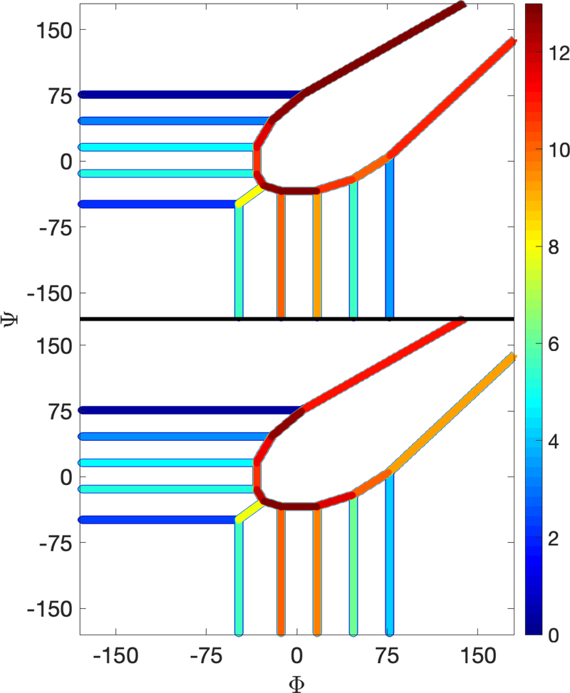
In Fig. 11 we show the free energy landscape that is obtained by the Milestoning calculation and the long-time trajectory. The free energy is a function of the milestone index α In other studies of the free energy (e.g. by umbrella sampling),²⁹ the free energy is given as a continuous function of the coarse coordinate(s) $\overrightarrow{Q},$ i.e. $F(\overrightarrow{Q})=-k_{B}T\log \left[P(\overrightarrow{Q})\right]$ where $P(\overrightarrow{Q})$ is the probability to find the system in the neighborhood of $\overrightarrow{Q}$. This probability is typically estimated by binning the number of times the trajectory is in the neighborhood of $\overrightarrow{Q}$. In Milestoning, the free energy is defined as $F_{\alpha }=-k_{B}T\log (P_{\alpha })$ where $P_{\alpha }$ is the probability that a trajectory crosses milestone $\alpha$ last. As a result, instantaneous configurations of a Milestoning trajectory can be anywhere in the two cells that are joined by the milestone of interest.

Fig 11.

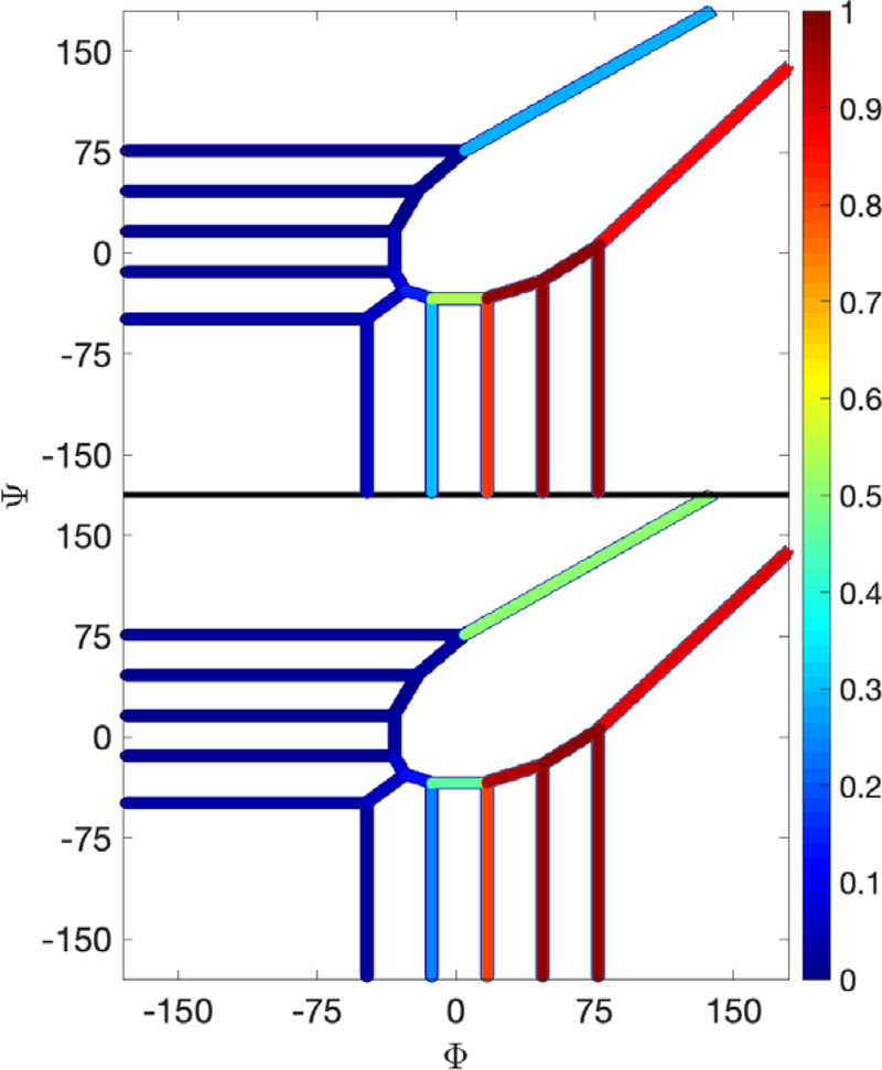
The color-coded free energy of the Milestones for alanine dipeptide in a vacuum. The lower panel shows the free energy extracted for a long MD trajectory. The upper figure shows the free energy extracted from exact Milestoning. The free energy is color-coded according to the right color panel. The free energy barrier is around $\mathrm{\Phi }\approx 0$ and is about 9 kcal/mol above the lowest energy.

Several milestones bind a cell. The configurations in the same cell may belong to trajectories that enter it via different milestones and therefore are in different states. In Milestoning the free energy is associated with a milestone and therefore configurations found in the same cell and at the same location can contribute free energy to different milestones. At the limit of small cell size, the Milestoning free energy is expected to converge to the usual free energy. However, for large cells (and large distances between milestones) the difference mentioned above should be kept in mind. To further emphasize this difference, we color-coded the free energy in Fig 4 and showed it only at the milestone. To make a meaningful comparison to exact and independent calculations, we considered the long and conventional MD trajectory, which was used to estimate the MFPT. We estimated from the long trajectory crossing events of milestones and compared the free energy landscape of this long trajectory to the landscape obtained from exact Milestoning.

Fig 4.

Continuation of the Milestoning input.txt with instructions to COLVAR and other simulation parameters.

Finally, we consider the committor function (Eq. 22) that is shown in Fig. 12. The committor function, $C_{\alpha },$ of milestone $\alpha$ is the probability that a trajectory initiated at $\alpha$ will make it to the product state before the reactant. It is used as a definition of an optimal reaction coordinate.² The committor function suggests that the space is divided roughly into two near $\varphi \approx 0,$ which is consistent with the significant free energy barrier (Fig. 11) that we find at a milestone near $\varphi \approx 0$. Interestingly the milestones of maximal free energy barrier and the milestone with a committor value of a half are different.

Fig. 12.

The committor function at the milestones for the alanine dipeptide conformational transition in a vacuum. Top panel: the committor value after 12 iterations of exact Milestoning. Lower panel: The committor estimated from a long MD trajectory.

The activated nature of the transition is clearly illustrated by the values of the committor function at the milestone. Essentially all the values of the committor are near zero at the negative value of the Φ dihedral angle. This observation suggests that the left part of the map consists of a single deep minimum. Every point in which we initiate a trajectory is very unlikely to continue to the product and is most likely to return to the reactant first. This is consistent with the free energy surface of alanine dipeptide in vacuum (Fig. 9) that includes a deep minimum for negative Φ values and also suggests a narrow channel leading from the reactants to products near $\mathrm{\Phi }\approx 0$ One of the advantageous of Milestoning is that the method provides a clear mechanism in addition to the time scale and the free energy landscape.

V.2. Alanine dipeptide in aqueous solution

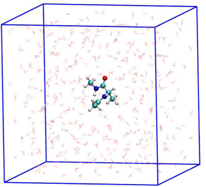
The system in this example is an alanine dipeptide and 448 water molecules (TIP3P³⁰) that are placed in a periodic box of an edge length of 25 Å (Fig 13). The simulations are conducted at constant temperature and volume to sample the initial conditions in the milestone (step 3 of the algorithm). The force field is again CHARMM22, and the algorithm of SHAKE²⁸ constrains all bonds that include hydrogen atoms. The cutoff distance for Lennard Jones interaction is 10 Å. The Ewald sum³¹ is used for electrostatic forces with a grid spacing of 1Å.

Fig. 13.

An alanine dipeptide solvated in a box of water that is used in the Milestoning calculations. See text for more details.

Interestingly, the presence of the solvent changes dramatically the free energy landscape of the dipeptide. The possibility to form hydrogen bonds with the solvent molecules reduces the stability of distorted internal hydrogen bonding that we found in vacuum and makes the $\alpha$-helix and the extended chain configurations stable.

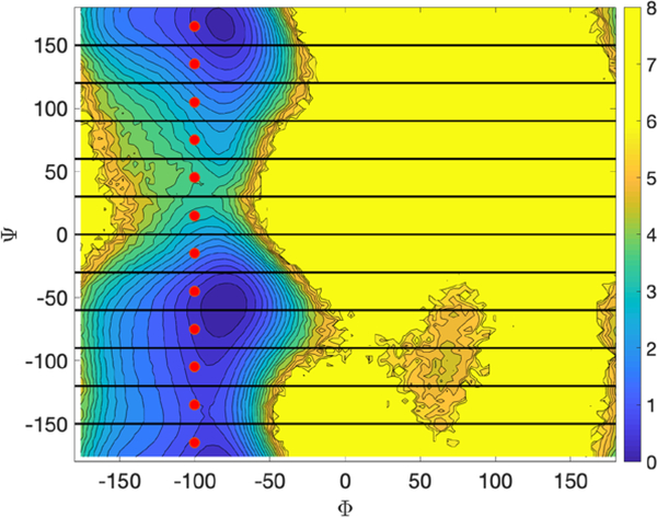
The solvated system is significantly larger than the system in vacuum. However, the description by coarse variables is more straightforward. Only the $\psi$ dihedral angle is required to describe the conformational transition. In Fig. 14 we show the anchors (red circles) and the milestones (black lines) on the precomputed $(\varphi ,\psi )$ free energy map. The detailed free energy contours are created from a one microsecond conventional MD simulation. The $(\varphi ,\psi )$ configurations along the trajectory are binned onto 90×90 grid to estimate the probability, $p(\mathrm{\Phi },\psi ).$ The logarithm of the estimated probabilities, $F=-kT\log \left[p(\mathrm{\Phi },\psi )\right]$ is the color-coded free energy in units of kcal/mol.

Fig. 14.

The free energy, $F(\mathrm{\Phi },\psi ),$ as a function of the dihedral angles $(\mathrm{\Phi },\psi )$ for a solvated alanine peptide. Also shown small red circles that are placed at the positions of the anchors. The horizontal black lines are the milestones. The reactant is defined at $\psi =-60$ and the product at $\psi =150$. The free energy is in kcal/mol.

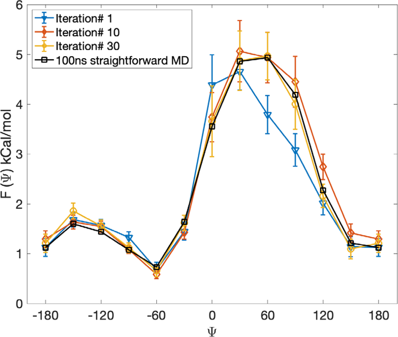
In Fig. 15 we show a one-dimensional free energy profile along the $\psi$ dihedral angle computed from Milestoning iteration (up to 30 iterations). We compare the profiles after one, ten and thirty iterations to a profile obtained from a conventional Molecular Dynamics trajectory of 100 nanosecond length. The simulations in solvent are shorter than in vacuum since the barrier height is significantly reduced compared to the system in vacuum. We obtain a semiquantitative agreement between Milestoning and conventional MD results. The high density of the milestones makes the comparison between the two approaches more meaningful.

Fig 15.

Free energy profiles for a solvated alanine dipeptide as a function of the dihedral angle ψ computed with exact Milestoning. Results are shown for different iteration numbers. Also shown are binned results from a single 100 nanosecond conventional MD trajectory. See text for a discussion about the difference between the Milestoning free energy and coordinate-based free energy.

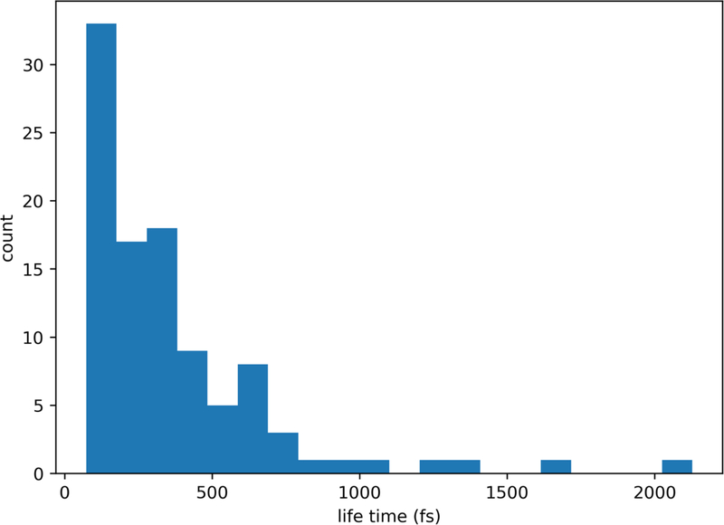
The maximal barrier height and location of the first iteration of Milestoning deviate from the results after ten and thirty iterations (and of the long MD trajectory). In contrast to earlier studies of alanine dipeptide with Milestoning^{15, 20} the trajectories between the milestones that we use here are exceptionally short. To illustrate their time distributions, we show in Fig. 16 the time distribution until termination of trajectories initiated from the milestone located at $\psi =60.$

Fig. 16.

The distribution of termination times of Milestoning trajectories starting at $\psi =60$ and ending at milestones directly accessible from it. While a small number of trajectories are longer than a picosecond, a significant fraction is shorter than 300 fs. This observation suggests that a single iteration of Milestoning (so-called “classical Milestoning”), will not be accurate for this set-up.

In an earlier reference ¹⁵, it was argued that Milestoning with a single iteration is likely to be adequate if the time scale of termination of unbiased trajectories between milestones is longer than velocity relaxation time. In that study, the velocity relaxation time was estimated to be about 300 fs. The distribution in Fig. 16 includes a large number of shorter trajectories leading to inaccurate estimates of kinetic and thermodynamic properties in the first iteration.

There are two solutions to this problem. The first solution is to increase the distances between the milestones (eliminate anchors that are too close to each other). The larger distances require more time to pass than in the original system and makes it more likely for the trajectories to reach a local equilibrium. This solution is the recommendation of reference ¹⁵ that we used extensively (for a recent review, see ¹). The second solution, which we use here, is to conduct exact Milestoning simulations. Exact Milestoning employs iterations on the interfaces or milestones. As the name suggests, exact Milestoning is not subject to local equilibrium conditions, provided that the observables converge to stable values. The convergence of the free energy as a function of the iteration number is therefore reassuring.

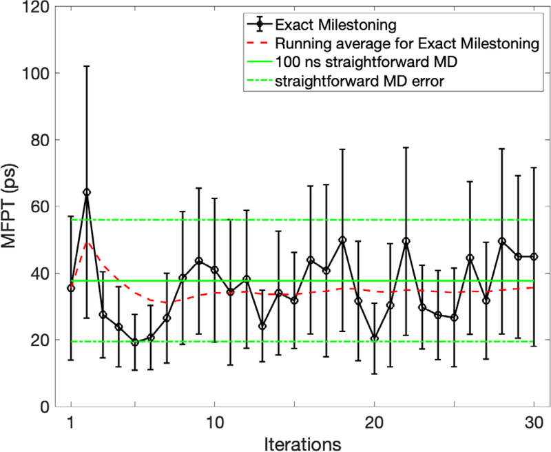
In Fig. 17 we show another major observable, the MFPT, as a function of the iteration number. The transition time scale ($40\pm 20ps$) is much shorter than in a vacuum due to a smaller barrier going backward through $\pm 180°$ (1–2 kcal/mol versus 9 kcal/mol in vacuum). The error bars of individual iterations are quite large. There are two sources of errors. The first source is the lack of convergence of the distribution in the milestone $f_{\alpha }^{(n)}(\overrightarrow{x}).$ This error is likely to cause a drift in the MFPT as a function of the iteration number. The second source is statistical errors due to a limited number of trajectories that reach a particular milestone. The error of the second source is likely to fluctuate near an average value. The value of the MFPT estimated by the Milestoning calculations fluctuates near a stable value after ~10 iterations. We, therefore, assume that the errors are mostly statistical and that the use of a running average for the MFPT (the red dashed line) is sound. The Milestoning running average is similar to the MFPT obtained from the straightforward MD trajectory.

Fig 17.

The MFPT for a conformational transition of a solvated alanine dipeptide between an alpha helix ($\psi =-60°$) and extended chain configuration ($\psi =150°$) as a function of the iteration number. We also show a red dashed line, which is a running average. The sampling at each milestone might be sparse even if the iterations converged. Therefore, the running average is a useful tool to reduce noise once the MFPT fluctuates near an average value as a function of the iteration index. The error bars were computed following section III.5.

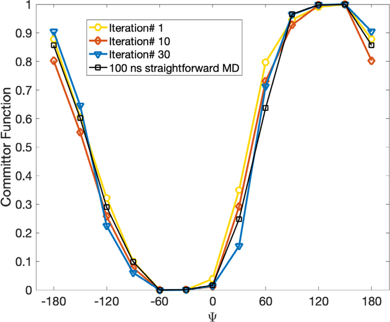
In Fig. 18 we show the committor values as a function of the dihedral angle ψ and the iteration number. Interestingly, all the curves are similar, including the results for Milestoning with one iteration. This observation suggests that the committor is less sensitive to local equilibrium compared to the free energy. Note that in the solvated simulations we did not impose a barrier at the edges of the map like we have done in vacuum. Transitions at the interface $\pm 180°$ can occur as the high value of the committor at the edge suggests. If the system is placed at $\psi =-90$ and attempts to reach $\psi =30$ it is more likely to do so by going ay through $\pm 180$. Hence, the barrier at positive $\psi$ values is not important for kinetics. The periodic boundary is an alternative and efficient pathway to connect the reactant at $\psi =-60$ with the product at $\psi =150$. The present example describes a diffusive motion over a barrier ~2kT (Fig. 15) in contrast to the activated dynamics of alanine dipeptide in vacuum.

Fig. 18.

Committor function for a solvated dipeptide as a function of the dihedral angle ψ computed with Milestoning with one iteration (classical Milestoning), exact Milestoning and from a straightforward MD simulation.

VI. Conclusions

We introduced a new python script to conduct Milestoning simulations. Milestoning is an algorithm and a theory to compute long-time molecular events and equilibrium features of complex molecular systems. The script is attached to the Molecular Dynamics engine NAMD and to the program COLVAR that handles coarse variables. It exploits the use of a large number of short trajectories, initiated at different locations in reaction space, to compute fluxes and kinetic observables. The simulation of multiple trajectories run in an automated fashion on a large number of computer nodes. It is, therefore, suitable for a modern computer architecture that exploits a large number of CPUs and cores. We divide the entire Milestoning run into several steps that can run as one process. A version of the script that runs in conjunction with the NAMD software¹³ can be found in GitHub https://github.com/UTweiw/ScMiles.

We further illustrate the use of the script on two simple examples: conformational transitions of alanine dipeptide in vacuum and in aqueous solution. Given the wide applicability of Milestoning in different and complex molecular systems (for a review see ¹) it is hoped that the script will ease the use of the theory and the algorithm by the broader community.

We finally comment that Milestoning is not a unique algorithm and software to study kinetics in complex biological systems, and alternatives are available. The NAMD¹³ package alone includes two other technologies to simulate kinetics. One is called SEEKR. It is based on multiscale dynamics that also exploits the Milestoning theory.³² It is an effective approach to study the kinetics of ligand binding to enzymes. The second approach that is found in NAMD is the adaptive multilevel splitting (AMS).³³ AMS is a successful approach to investigate exact stochastic dynamics along a one-dimensional reaction coordinate. The ScMiles software is different from the above two in its generality. ScMiles can investigate a wide range of problems that include conformational transition in proteins³⁴, passive membrane transport²⁴, and others.^{26, 35} These studies are conducted with a variety of coarse variables and in can be executed in multiple dimensions. The generality makes it more challenging to adapt ScMiles to different applications. However, the flexibility of ScMiles can also be useful. Essentially, the same procedure is effective for diverse problems.

The AMS approach is based on the exploitation of a single coarse variable. It uses exact stochastic dynamics to generate complete trajectories from reactant to product. The time of the complete trajectories must be accessible to conventional MD. The generation of full trajectories restricts its application to activated dynamics in which the reactive trajectories are fast (but rare). For this class of problems, the AMS is an attractive solution. In contrast to AMS, Milestoning does not generate complete trajectories. It generates the overall flux by iterations of short trajectories at the milestones. The use of short trajectories is more efficient than the use of complete trajectories. However, the use of milestones comes at the cost of approximating the distributions $f_{\alpha }^{(n)}$ which needs to be improved by iterations.

If the distributions, $f_{\alpha }^{(n)},$ can be sampled quickly and accurately, Milestoning is an efficient approach. If, however, the distributions are hard to generate, like in systems far from equilibrium, the calculations with Milestoning will be challenging computationally. At present, simulations of system far from equilibrium is challenging to other methods as well.

Fig. 5.

A sample input for COLVAR as used in Milestoning. The atomic indices are for the particles that define the coarse variable.

References

- 1.Elber R, A new paradigm for atomically detailed simulations of kinetics in biophysical systems. Q. Rev. Biophys. 2017, 50, 1–15 [DOI] [PubMed] [Google Scholar]
- 2.E, W. N.; Vanden-Eijnden E , Transition-Path Theory and Path-Finding Algorithms for the Study of Rare Events. Annu. Rev. Phys. Chem, 2010, 61, 391–420. [DOI] [PubMed] [Google Scholar]
- 3.Bolhuis PG; Chandler D; Dellago C; Geissler PL, Transition path sampling: Throwing ropes over rough mountain passes, in the dark. Annu. Rev. Phys. Chem. 2002, 53, 291–318. [DOI] [PubMed] [Google Scholar]
- 4.Zhang BW; Jasnow D; Zuckerman DM, The “weighted ensemble” path sampling method is statistically exact for a broad class of stochastic processes and binning procedures. J. Chem. Phys. 2010, 132, 5. [DOI] [PMC free article] [PubMed] [Google Scholar]
- 5.Dinner AR; Mattingly JC; Tempkin JOB; van Koten B; Weare J, Trajectory Stratification of Stochastic Dynamics. Siam Rev. 2018, 60, 909–938. [DOI] [PMC free article] [PubMed] [Google Scholar]
- 6.Bowman GR; Pande VS, An Introduction to Markov State Models and Their Applictaions to Long Timescale Molecular Simulations. Springer; Heidelberg, 2014; p 139. [Google Scholar]
- 7.Shaw DE; Deneroff MM; Dror RO; Kuskin JS; Larson RH; Salmon JK; Young C; Batson B; Bowers KJ; Chao JC; Eastwood MP; Gagliardo J; Grossman JP; Ho CR; Ierardi DJ; Kolossvary I; Klepeis JL; Layman T; McLeavey C; Moraes MA; Mueller R; Priest EC; Shan YB; Spengler J; Theobald M; Towles B; Wang SC, Anton, a special-purpose machine for molecular dynamics simulation. Comm. ACM 2008, 51, 91–97. [Google Scholar]
- 8.Dellago C; Bolhuis PG, Transition path sampling simulations of biological systems. In Atomistic Approaches in Modern Biology: from Quantum Chemistry to Molecular Simulations, 2007; 268, 291–317. [Google Scholar]
- 9.Faradjian AK; Elber R, Computing time scales from reaction coordinates by milestoning. J. Chem. Phys. 2004, 120, 10880–10889. [DOI] [PubMed] [Google Scholar]
- 10.Moroni D; Bolhuis PG; van Erp TS, Rate constants for diffusive processes by partial path sampling. J. Chem. Phys. 2004, 120, 4055–4065. [DOI] [PubMed] [Google Scholar]
- 11.Bello-Rivas JM; Elber R, Exact milestoning. J. Chem. Phys. 2015, 142,094102. [DOI] [PMC free article] [PubMed] [Google Scholar]
- 12.Huber GA; Kim S, Weighted-ensemble Brownian dynamics simulations for protein association reactions. Biophys. J. 1996, 70, 97–110. [DOI] [PMC free article] [PubMed] [Google Scholar]
- 13.Phillips JC; Braun R; Wang W; Gumbart J; Tajkhorshid E; Villa E; Chipot C; Skeel RD; Kale L; Schulten K, Scalable molecular dynamics with NAMD. J. Comput. Chem. 2005, 26, 1781–1802. [DOI] [PMC free article] [PubMed] [Google Scholar]
- 14.Noe F; Horenko I; Schutte C; Smith JC, Hierarchical analysis of conformational dynamics in biomolecules: transition networks of metastable states. J. Chem. Phys. 2007, 126, 155102. [DOI] [PubMed] [Google Scholar]
- 15.West AMA; Elber R; Shalloway D, Extending molecular dynamics time scales with milestoning: Example of complex kinetics in a solvated peptide. J. Chem. Phys. 2007, 126, 145104. [DOI] [PubMed] [Google Scholar]
- 16.Reimann P; Schmid GJ; Hanggi P, Universal equivalence of mean first-passage time and Kramers rate. Phys. Rev. E 1999, 60, R1–R4. [DOI] [PubMed] [Google Scholar]
- 17.Vanden Eijnden E; Venturoli M; Ciccotti G; Elber R, On the assumption underlying Milestoning. J. Chem. Phys. 2008, 129, 174102. [DOI] [PMC free article] [PubMed] [Google Scholar]
- 18.Elber R; Bello-Rivas MJ; Ma P; Cardenas AE; Fathizadeh A, Calculating Iso-Committor Surfaces as Optimal Reaction Coordinates with Milestoning. Entropy 2017, 19, 219. [DOI] [PMC free article] [PubMed] [Google Scholar]
- 19.Vanden-Eijnden E; Venturoli M, Markovian milestoning with Voronoi tessellations. J. Chem. Phys. 2009, 130, 13. [DOI] [PubMed] [Google Scholar]
- 20.Majek P; Elber R, Milestoning without a reaction coordinate. J. Chem. Theory Comput. 2010, 6, 1805–1817. [DOI] [PMC free article] [PubMed] [Google Scholar]
- 21.Elber R, A milestoning study of the kinetics of an allosteric transition: Atomically detailed simulations of deoxy Scapharca hemoglobin. Biophys. J. 2007, 92, L85–L87. [DOI] [PMC free article] [PubMed] [Google Scholar]
- 22.Boninsegna L; Gobbo G; Noe F; Clementi C, Investigating Molecular Kinetics by Variationally Optimized Diffusion Maps. J. Chem. Theory Comput. 2015, 11, 5947–5960. [DOI] [PubMed] [Google Scholar]
- 23.Fiorin G; Klein ML; Hénin J, Using collective variables to drive molecular dynamics simulations. Mol. Phys. 2013, 111, 3345–3362. [Google Scholar]
- 24.Fathizadeh A; Elber R, Ion Permeation through a Phospholipid Membrane: Transition State, Path Splitting, and Calculation of Permeability. J. Chem. Theory Comput. 2019, 15, 720–730. [DOI] [PMC free article] [PubMed] [Google Scholar]
- 25.Kirmizialtin S; Nguyen V; Johnson KA; Elber R, How Conformational Dynamics of DNA Polymerase Select Correct Substrates: Experiments and Simulations. Structure 2012, 20, 618–627. [DOI] [PMC free article] [PubMed] [Google Scholar]
- 26.Ma P; Cardenas AE; Chaudhari MI; Elber R; Rempe SB, The Impact of Protonation on Early Translocation of Anthrax Lethal Factor: Kinetics from Molecular Dynamics Simulations and Milestoning Theory. J. Am. Chem. Soc. 2017, 139, 14837–14840. [DOI] [PMC free article] [PubMed] [Google Scholar]
- 27.Huang J; Rauscher S; Nawrocki G; Ran T; Feig M; de Groot BL; Grubmuller H; MacKerell AD, CHARMM36: An Improved Force Field for Folded and Intrinsically Disordered Proteins. Biophys. J. 2017, 112, 175A–176A. [DOI] [PMC free article] [PubMed] [Google Scholar]
- 28.Ryckaert JP; Ciccotti G; Berendsen HJC, Numerical Integration of Cartesian Equations of Motion of a System with Constraints - Molecular Dynamics of N-Alkanes. J. Comp. Phys. 1977, 23, 327–341. [Google Scholar]
- 29.Valleau J, Monte Carlo: changing the rules for fun and profit In Classical and quantum dynamics in condensed phase simulations, Berne Bruce J., G. C., and David F. Coker, Ed. World Scientific: Singapore, 1998. [Google Scholar]
- 30.Jorgensen WL; Chandrasekhar J; Madura JD; Impey RW; Klein ML, Comparison of Simple Potential Functions for Simulating Liquid Water. J. Chem. Phys. 1983, 79, 926–935. [Google Scholar]
- 31.Essmann U; Perera L; Berkowitz ML; Darden T; Lee H; Pedersen LG, A Smooth Particle Mesh Ewald Method. J. Chem. Phys. 1995, 103, 8577–8593. [Google Scholar]
- 32.Jagger BR; Lee CT; Amaro RE, Quantitative Ranking of Ligand Binding Kinetics with a Multiscale Milestoning Simulation Approach. J. Phys. Chem. Lett. 2018, 9, 4941–4948. [DOI] [PMC free article] [PubMed] [Google Scholar]
- 33.Lopes LJS; Lelievre T, Analysis of the Adaptive Multilevel Splitting Method on the Isomerization of Alanine Dipeptide. J. Comput. Chem. 2019, 40, 1198–1208. [DOI] [PubMed] [Google Scholar]
- 34.Kirmizialtin S; Johnson KA; Elber R, Enzyme Selectivity of HIV Reverse Transcriptase: Conformations, Ligands and Free Energy Partitions. J. Phys. Chem. B 2015, 119,11513–11526. [DOI] [PMC free article] [PubMed] [Google Scholar]
- 35.Templeton C; Elber R, Why Does RNA Collapse? The Importance of Water in a Simulation Study of Helix–Junction–Helix Systems. J. Am. Chem. Soc. 2018, 140, 16948–16951. [DOI] [PMC free article] [PubMed] [Google Scholar]