Model evaluation for the prediction of solubility of active pharmaceutical ingredients (APIs) to guide solid–liquid separator design

Graphical Abstract

A guide for the selection of predictive models is provided, which considers various solute and solvent properties, such as molecular mass, functional group diversity and hydrophobia/hydrophilia

Abstract

The assumptions and models for solubility modelling or prediction in systems using non-polar solvents, or water and complex triterpene and other active pharmaceutical ingredients as solutes aren't well studied. Furthermore, the assumptions concerning heat capacity effects (negligibility, experimental values or approximations) are explored, using non-polar solvents (benzene), or water as reference solvents, for systems with solute melting points in the range of 306–528 K and molecular weights in the range of 90–442 g/mol. New empirical estimation methods for the ${\Delta }_{fus}{C}_{pi}$ of APIs are presented which correlate the solute molecular masses and van der Waals surface areas with ${\Delta }_{fus}{C}_{pi}$. Separate empirical parameters were required for oxygenated and non-oxygenated solutes. Subsequently, the predictive capabilities of the various approaches to solubility modelling for complex pharmaceuticals, for which data is limited, are analysed. The solute selection is based on a principal component analysis, considering molecular weights, fusion temperatures, and solubilities in a non-polar solvent, alcohol, and water, where data was available. New NRTL-SAC parameters were determined for selected steroids, by regression. The original UNIFAC, modified UNIFAC (Dortmund), COSMO-RS (OL), and COSMO-SAC activity coefficient predictions are then conducted, based on the availability of group constants and sigma profiles. These are undertaken to assess the predictive capabilities of these models when each assumption concerning heat capacity is employed. The predictive qualities of the models are assessed, based on the mean square deviation and provide guidelines for model selection, and assumptions concerning phase equilibrium, when designing solid–liquid separators for the pharmaceutical industry on process simulation software. The most suitable assumption regarding ${\Delta }_{fus}{C}_{pi}$ was found to be system specific, with modified UNIFAC (Dortmund) performing well in benzene as a solvent system, while original UNIFAC performs better in aqueous systems. Original UNIFAC outperforms other predictive models tested in the triterpene/steroidal systems, with no significant influence from the assumptions regarding ${\Delta }_{fus}{C}_{pi}$.

1. Introduction

The separation and purification of pharmaceutical products, or intermediates, are arguably the most important and cost intensive process steps in the pharmaceutical industry. The method, degree and efficiency of the process are generally dictated by the phase behaviour of the solute. Kolář et al. [1] state that over 30% of the efforts of industrial property modellers and experimentalists deal with solvent selection. It is therefore imperative that appropriate solvents are analytically selected, based on broadly-sourced information that may include phase equilibrium experimental data, reliable predictions, experience and solute theory (e.g. structure, bonds and physical properties).

Often it is not possible to determine the phase behaviour of these systems experimentally, as small amounts of each pharmaceutical product are manufactured in the initial stages of design and synthesis. Due to this constraint, many thermodynamic models have been applied to predict the solubility via predictive Gibbs excess energy models. These models include functional group approaches such as UNIFAC [2], modified UNIFAC (Dortmund) [3], and surface segment approach models, such as COSMO-RS (OL) [4], COSMO-SAC [5] and NRTL-SAC [6] and have exhibited varying degrees of success in predicting the solubility of common pharmaceutical compounds with relatively simple molecular structures [6], [7], [8], [9], [10]. Gmehling et al. [7] and Gracin et al. [8] have explored the ability of the UNIFAC model to predict solid–liquid equilibria. Gmehling et al. [7] considered relatively simple ring structured solutes such as naphthalene and anthracene. The authors could provide good estimates by UNIFAC predictions for the systems considered. Gracin et al. [8] used the UNIFAC model to predict solubilities of single-ring pharmaceuticals such as ibuprofen and aspirin. The authors concluded that accurate predictions were not achievable, and suggested the use of the UNIFAC model for initial estimates only.

Hahnenkamp et al. [11] have evaluated and compared the predictive capabilities of the models of Fredenslund et al., Weidlich and Gmehling, Grensemann and Gmehling, and Lin and Sandler [2], [3], [4], [5] for systems containing ibuprofen and aspirin. The authors determined that the predictions of the model presented in Weidlich and Gmehling [3] provided the lowest deviations from the experimental data, when compared to the models from Fredenslund et al. [2] and Grensemann and Gmehling [4]. Diedrichs and Gmehling [12] conducted a detailed model comparison, but only systems with alcohol, alkane, or water as a solvent, were considered. Furthermore, systems with solute mole fractions greater than 0.1 were excluded in the comparison. Schröder et al. [13] explored the prediction of aqueous solubilities of various solid carboxylic acids that are used in the pharmaceutical industry.

Little work on the abilities of predictive models for the solubility of complex pharmaceuticals, such as polycyclic aromatics, specifically steroidal triterpenes, is available in the literature. This is mainly due to a lack of experimental data which is imperative to generate model-specific parameters that are usually essential for the application of most predictive models. It is however important that accurate predictions can be made without an extensive set of experimental data, as this would obviously limit the practicality of the predictive model. Abildskov et al. [14] have provided some satisfactory predictions for a limited set of steroidal molecules by conducting sensitivity tests on UNIFAC model parameters however this data is incomplete and not readily available.

In this work, the various aforementioned predictive models were tested to determine the most accurate method for solubility modelling for the solutes considered. The models were chosen based on the variations in the approach to solubility modelling (functional group based, segment based, reference solvent based). The differences in combinatorial and residual expressions are distinguished. The results of the predictions are intended to provide qualitative estimates of solubility data as the predictive models generally yield poor quantitative results in the case of solid–liquid equilibria. The performance of the models is correlated with the molecular surface area, molecular weight, and functional group diversity. In this work, functional group definitions based on the work of Fredenslund et al. [2] were used.

In addition, the works of Mishra and Yalkowsky [15] and Neau et al. [16] are explored for complex steroidal systems in benzene, or water, as hydrophobic and hydrophilic reference solvents. This is to determine the effect, of the assumption of zero or non-zero-approximates/experimental data, on changes in heat capacity upon fusion in systems exhibiting ideal solubility in the solid phase. Neau et al. [16] showed that the assumption of negligible heat capacity changes can cause large errors in calculated solubility, during modelling for solutes of melting points exceeding 420 K. However, an ideal liquid phase was assumed in their work. Hence, the effect of the activity coefficient was not considered. The tests of Neau et al. [16] have been limited to solute melting points of 470 K, where the different assumptions for changes in heat capacity can result in deviations from experimental data of up to 27%. The effect of the increasing difference between the experimental solubility temperature and fusion temperature is tested in this work.

The range of solute melting points considered in the test set here exceeds 520 K, with molecular weights in the range of 90–442 g/mol. It is also useful to establish differences (if any) in performance due to the solvent involved (non-polar organic vs. aqueous). The effect of the various methods of dealing with changes in heat capacity, between the solid and liquid solute ($\Delta C_p$) on the predicted solubility, are explored, in conjunction with the different predictive models for the activity coefficient, from the literature. This is to determine the most suitable combination of combinatorial and residual activity coefficient model terms, along with the most suitable model equation for solubility prediction.

2. Theory

The activity coefficient is a measure of the non-ideality of solutions [12]. The parameter is a strong function of composition, and of temperature to a degree, but is weakly dependent on pressure, at low to moderate pressures. In some cases, the activity coefficient is greater than 1, however, values below 1 are common in solvating systems (as shown in Gmehling et al. [7]), such as solutions of phenol and alkanols or alkanes and polymers. Usually, the degree of dissimilarity between component sizes comprising a mixture is proportional to the differences in activity coefficients of those components [6].

2.1. Solid–liquid phase equilibrium

At solid–liquid phase equilibrium, the solvent is saturated with the solute. In the case of eutectic mixtures, the solubility of the solvent in the solid solute is neglected, and the chemical potential of the solute, i, in the pure solid phase ${\mu }_i^s$, is equal to the chemical potential of the solute in the liquid solution, ${\mu }_i^{sat}$ as shown by Bouillot et al. [10]:

$${\mu }_i^s={\mu }_i^{sat}$$ (1)

The chemical potential of the solute in the liquid solution can be expressed as:

$${\mu }_i^{sat}={\mu }_i^0+RTl\mathrm{n}\left({\gamma }_i^{sat}{x}_i^{sat}\right)$$ (2)

where, ${\mu }_i^0$, is the chemical potential of the hypothetical pure liquid solute at system temperature (reference state), T is the tempearture in Kelvin, R is the universal gas constant in J/mol∙K and ${\gamma }_i^{sat}$ is the activity coefficient of the solute in the saturated solution.

The activity $\left(a_i^{sat}={\gamma }_i^{sat}{x}_i^{sat}\right)$of the solute can be determined by combining Equations (1) and (2), yielding:

$$ln\left({\gamma }_i^{sat}{x}_i^{sat}\right)=\frac{{\mu }_i^s-{\mu }_i^0}{RT}$$ (3)

At constant temperature and pressure, the chemical potential is equal to the partial molar Gibbs energy, so that:

$$\frac{{\mu }_i^{sat}-{\mu }_i^0}{RT}=\frac{{\overline{G}}_i^s-{\overline{G}}_i^0}{RT}$$ (4)

And hence

$$ln\left({\gamma }_i^{sat}{x}_i^{sat}\right)=\frac{{\Delta }_{fus}{\overline{G}}_i^m}{RT}$$ (5)

where ${\Delta }_{fus}{\overline{G}}_i^m$ is the hypothetical partial molar Gibbs energy of melting at the system temperature and pressure [10], which is zero for the pure solute at its melting point. Assuming a constant difference in heat capacity, between the solid and the subcooled liquid solute, between the triple point and the system temperature, the following expression can be derived:

$$\frac{{\Delta }_{fus}{\overline{G}}_i^m\left(T\right)}{RT}=\frac{{\Delta }_{fus}{H}_i\left(T_{tr}\right)}{R}\left(\frac{1}{T_{tr}}-\frac{1}{T}\right)-\frac{{\Delta }_{fus}{C}_{pi}}{R}\left[ln\left(\frac{T_{tr}}{T}\right)-\frac{T_{tr}}{T}+1\right]$$ (6)

where ${\Delta }_{fus}{H}_i\left(T_{tr}\right)$ is the enthalpy of fusion at the triple point, $T_{tr}$ is the triple point temperature in Kelvin, and ${\Delta }_{fus}{C}_{pi}$is the difference in heat capacity between the subcooled liquid solute and the solid.

This derivation disregards the pressure influence on solid solubility, as the difference between system pressure, and triple point pressure, is regarded as sufficiently small, so that a Poynting correction term is not required. Hence the triple point at 1 atmosphere (${}_{fus}{T}_i$) is often used as a substitute, due mainly to the greater abundance of this data.

Often the effect of ${\Delta }_{fus}{C}_{pi}$is assumed to be small in comparison to the other term, and is omitted. This assumtion is only valid when the SLE temperature is similar to the triple point temperature.

Equation (6) then reduces to:

$$\frac{{\Delta }_{fus}{G}_i\left({}_{fus}{T}_i\right)}{RT}=\frac{{\Delta }_{fus}{H}_i\left({}_{fus}{T}_i\right)\left({}_{fus}{T}_i\right)}{R}\left(\frac{1}{{}_{fus}{T}_i}-\frac{1}{T}\right)$$ (7)

Hildebrand and Scott [17], [18] however, recommend estimating the ${\Delta }_{fus}{C}_{pi}$ as $\frac{{\Delta }_{fus}{H}_i}{{}_{fus}{T}_i}$ yielding:

$$ln\left({\gamma }_i^l{x}_i^l\right)=\frac{{\Delta }_{fus}{G}_i}{RT}=\frac{{\Delta }_{fus}{H}_i}{R_{fus}{T}_i}ln\left(\frac{T}{{}_{fus}{T}_i}\right)$$ (8)

This improvement has been supported by Neau et al. [16], and is explored further in this work.

2.2. Predictive activity coefficient models

A brief description of the predictive activity coefficient models used follows. The reader is referred to the original publications for an in-depth discussion [2], [3], [4], [5], [6].

2.2.1. The UNIFAC and modified UNIFAC (Dortmund) model

The UNIFAC activity coefficient model, introduced by Fredenslund et al. [2], makes two contributions to the activity coefficient. Namely a combinatorial (accounting for size shape interactions), and residual (acounting for energetic interactions), component.

$$ln{\gamma }_i=ln{\gamma }_i{}^{\mathit{comb}}+ln{\gamma }_i{}^{res}$$ (9)

where, $ln{\gamma }_i{}^{\mathit{comb}}$, and, $ln{\gamma }_i{}^{res}$, are the combinatorial, and residual contributions, respectively, and are given by the following expressions:

$$ln{\gamma }_i{}^{\mathit{comb}}=ln\left(\frac{{\Phi }_i}{x_i}\right)+1-\left(\frac{{\Phi }_i}{x_i}\right)-\frac{Z}{2}{q}_i\left(ln\frac{{\Phi }_i}{{\vartheta }_i}+1-\frac{{\Phi }_i}{{\vartheta }_i}\right)$$ (10)

where

$${\vartheta }_i=\frac{x_i{q}_i}{x_i{q}_i+x_j{q}_j}=\frac{x_i{q}_i}{q}$$ (11)

and

$${\Phi }_I=\frac{x_i{r}_i}{x_i{r}_i+x_j{r}_j}=\frac{x_i{r}_i}{r}$$ (12)

where, r_i, and, q_i, are the molecular volume and surface area, and Z is the coordination number. For the original UNIFAC model, the molecular volume and surface area are estimated from the group contribution values of ref. [19].

The residual term, $ln{\gamma }_i{}^{res}$, is evaluated from group contributions:

$$ln{\gamma }_i{}^{res}={\displaystyle {\sum }_k{\nu }_k^{\left(i\right)}\left(ln{\Gamma }_k-ln{\Gamma }_k^{\left(i\right)}\right)}$$ (13)

where ${\nu }_k^{\left(i\right)}$ is the number of functional groups of the type, k, in a molecule of component, i, and $ln{\Gamma }_k^{\left(i\right)}$ is the residual contribution to the activity coefficient by the functional group, k, in the pure fluid, i. Since the pure fluid, i, is also a mixture of groups, the term, $ln{\Gamma }_k^{\left(i\right)}$, is incorporated to reduce the residual term of the pure fluid to zero.

The contribution to the residual portion of the activity by the functional group, k, is given by the following relationship:

$${\Gamma }_k=exp\left(Q_k\left[1-ln\left({\displaystyle {\sum }_m{\Theta }_m{\Psi }_{mk}}\right)-{\displaystyle {\sum }_m\frac{{\Theta }_m{\Psi }_{km}}{{\displaystyle {\sum }_n{\Theta }_n{\Psi }_{nm}}}}\right]\right)$$ (14)

where ${\Theta }_m$ is the surface area fraction of the functional group, m, in the mixture. The binary interaction parameter is between groups, m and n, while a_mn is accounted for through the parameter, ${\Psi }_{mn}$, where:

$${\Psi }_{mn}=\exp \left(-\frac{a_{mn}}{T}\right)$$ (15)

T is the system temperature in Kelvin.

As mentioned above, the expression for ${\Gamma }_k$, presented in Equation (14), includes the functional group, k, contributions to activity, of both the mixture and the pure fluid.

Several modifications to the original UNIFAC model have been proposed, with the most significant modifications made to the expression for the temperature dependence of binary interaction parameters, and the introduction of different combinatorial expressions, with unique group volume and area parameters, as well as component group fragmentations.

In the modified UNIFAC (Dortmund) [3] a quadratic temperature dependence of the binary interaction parameter, $a_{mn}$, is proposed:

$$a_{mn}=a_{mn,0}+a_{mn,1}T+a_{mn,2}{T}^2$$ (16)

Additionally, the combinatorial expression is given by:

$$ln{\gamma }_i{}^{\mathit{comb}}=ln\left(\frac{\phi {\prime }_i}{x_i}\right)+1-\frac{\phi {\prime }_i}{x_i}-\frac{Z}{2}{q}_i\left(ln\frac{{\Phi }_i}{{\vartheta }_i}+1-\frac{{\Phi }_i}{{\vartheta }_i}\right)$$ (17)

where

$$\phi {\prime }_i=\frac{x_i{r}_i^{3/4}}{{\displaystyle {\sum }_j{x}_j{r}_j^{3/4}}}$$ (18)

$${\Phi }_i=\frac{x_i{r}_i}{{\displaystyle {\sum }_j{x}_j{r}_j}}$$ (19)

The parameters of r and q are determined by data fitting, and not from the method of Bondi (1964).

The modified UNIFAC (Dortmund) model was adapted further, for application to pharmaceutical systems, by Diedrichs and Gmehling [12]. This model was termed Pharma Modified UNIFAC. It was assumed, in that work, that certain functional group contributions become irrelevant in solutions of pharmaceutical molecules in common solvents, if the solubility is low, and can therefore be omitted. A unique group-fragmentation scheme is used in this model. Promising results for limited classes of solvents were obtained [12]. The model is however limited in applicability to a solute mole fraction of less than 0.1.

2.2.2. The COSMO-RS, COSMO-SAC and COSMO-RS (OL) models

Generally, the activity coefficient of a mixture is determined through the Gibbs excess energy function. Klamt [20] proposed a means of determining the activity coefficient, using chemical potentials from surface shielding charge densities determined by quantum-mechanical calculations. The Conductor-like Screening Model for Real Solvents (COSMO-RS) was introduced, as an a priori predictive model, and an alternative to the traditional group contribution-based models.

In COSMO-RS, molecules of a solute–solvent system are treated as a combination of molecular-shaped, cavity surface segments. The concept involves modelling the placement of a “cavity” that is a replica of a molecule of the solute, with zero charge, inside the homogeneous theoretical solvent, with a fixed dielectric constant, ε. The energy change involved in this placement represents a component of the total Gibbs energy change of solvation. The replica molecule charges are then replaced, yielding a realistic solute. The energy change associated with this is the second contributor to the Gibbs energy change of solvation. To know how charges must be replaced, each shielding charge density (σ) must be characterized by a “sigma profile”.

COSMO-RS (OL) is the in-built Dortmund Data Bank-modified version of the COSMO-RS model. The most significant modification to the model, in this version, includes an empirical correction term for hydrogen bonding, which is suggested to be over-compensated for in non-hydrogen bonding mixtures, in the original COSMO-RS model. The specifics of this modification are outlined in the original publication [4].

Lin and Sandler [5] have proposed some modifications to the original COSMO-RS model. The authors have stated that the expression for the chemical potential, given by ref. [20], does not converge with certain boundary conditions, and that the expression for the activity coefficient presented, does not satisfy certain thermodynamic consistency tests.

The modifications of Lin and Sandler [5] result in the Conductor-like Screening Model-Segment Activity Coefficient model (COSMO-SAC), which is reviewed here.

The derivation of the expression of the activity coefficient using the COSMO-SAC model is extensive and beyond the scope of this work, but the reader is referred to the original publications for both the COSMO-RS [4], [20] and COSMO-SAC [5] models for further details. The final expression for the activity coefficient of solute, i, in solvent S, $ln{\gamma }_{i/S}$, using the COSMO-SAC model is given by:

$$ln{\gamma }_{i/S}=n_i{\displaystyle {\sum }_{{\sigma }_m}{p}_i\left({\sigma }_m\right)\left[ln{\Gamma }_S\left({\sigma }_m\right)-ln{\Gamma }_i\left({\sigma }_m\right)\right]}+ln{\gamma }_{i/S}{}^{SG}$$ (20)

where n_i, is the total number of segments contributed by molecule, i. ${\sigma }_m$, is the surface charge density of segment, m, and, $p_i\left({\sigma }_m\right)$, is the frequency of surface charge density, m, of component, i, given by:

$$p_i\left({\sigma }_m\right)=\frac{n_i\left({\sigma }_m\right)}{n_i}$$ (21)

where $n_i\left({\sigma }_m\right)$, is the total number of segments in component, i, with charge density, ${\sigma }_m$. $ln{\Gamma }_S\left({\sigma }_m\right)$, is the segment activity coefficient in the mixture for segments with charge density,${\sigma }_m$, given by:

$$ln{\Gamma }_S\left({\sigma }_m\right)=-ln\left\{{\displaystyle {\sum }_{{\sigma }_n}{p}_s\left({\sigma }_n\right){\Gamma }_S\left({\sigma }_n\right)exp\left[\frac{-\Delta W\left({\sigma }_m\text{},{\sigma }_n\right)}{kT}\right]}\right\}$$ (22)

where $\Delta W$, is the exchange energy and k, is the Boltzmann constant. $ln{\Gamma }_i\left({\sigma }_m\right)$, is the segment activity coefficient in the pure component, i, for segments with charge density, ${\sigma }_m$. $ln{\gamma }_{i/S}{}^{SG}$, is the Staverman–Guggenheim [21], [22] combinatorial term given by:

$$ln{\gamma }_{i/S}{}^{SG}=ln\frac{{\varphi }_i}{x_i}+\frac{Z}{2}{q}_{i}ln\frac{{\vartheta }_i}{{\varphi }_i}+l_i-\frac{{\varphi }_i}{x_i}{\displaystyle {\sum }_{j=1}^n{x}_j{l}_j}$$ (23)

where ${\vartheta }_i$, is the surface area fraction given by:

$${\vartheta }_i=\frac{q_i{x}_i}{{\displaystyle {\sum }_j{q}_j{x}_j}}$$ (24)

where ${\varphi }_i$, is the volume fraction parameter given by:

$${\varphi }_i=\frac{r_i{x}_i}{{\displaystyle {\sum }_j{r}_j{x}_j}}$$ (25)

and

$$l_i=\frac{z}{2}\left(r_i-q_i\right)-\left(r_i-1\right)$$ (26)

2.2.3. Non-random two liquid segment activity coefficient model (NRTL-SAC)

The NRTL-SAC [6], [23] model, is based on the polymer NRTL model by Chen [24], and was developed specifically for the use in the modelling of the activity of complex molecules, such as pharmaceuticals. The non-ideality is accounted for based on “contributions” from four different conceptual segments that make up a particular component. These include polar-positive, polar-negative, hydrophobic and hydrophilic segments. Each molecular surface is conceptually divided into these segments, in different proportions of the molecular surface area. Every molecule is thus designated a conceptual segment surface “composition”. The surface interactions between pairs of segments are accounted for through constant binary interaction parameters only.

The main differences between the original NRTL model of Renon and Prausnitz [25], and the NRTL-SAC model, include the concept of segment interaction, and the addition of a combinatorial term, as size/shape interactions become considerable in larger complex molecules. Additionally, the NRTL-SAC model has no in-built temperature dependency.

The combinatorial term of Flory–Huggins [26], [27], is used in the model. The subscripts, A and B, are used to denote pure components, whereas the subscripts, i, j, k, m, and, m′, are used to represent segment-based species indices.

$$ln{\gamma }_A^{\mathit{Comb}}=ln\frac{{\varphi }_A}{x_A}+1-r_A{\displaystyle {\sum }_B\frac{{\varphi }_B}{r_B}}$$ (27)

where

$$r_A={\displaystyle {\sum }_i{r}_{i,A}}$$ (28)

$${\varphi }_A=\frac{x_A{r}_A}{{\displaystyle {\sum }_B{x}_B{r}_B}}$$ (29)

where $r_A$, is the total number of segments, i, in component, A, and, ${\varphi }_A$, is the segment mole fraction of component, A.

The residual term is identical to that of the polymer NRTL [24] where:

$$ln{\gamma }_A^{\mathrm{Re}s}=ln{\gamma }_A^{lc}={\displaystyle {\sum }_m{r}_{m,A}\left[ln{\Gamma }_m^{lc}-ln{\Gamma }_m^{lc,A}\right]}$$ (30)

where $ln{\Gamma }_m^{lc}$, is the segment activity coefficient of species, m, in the mixture, and, $ln{\Gamma }_m^{lc,A}$, is the segment activity coefficient of species, m, in the pure component, A, and these are calculated from the following relations:

$$ln{\Gamma }_m^{lc}=\frac{{\displaystyle {\sum }_j{x}_j{G}_{jm}{\tau }_{jm}}}{{\displaystyle {\sum }_k{x}_k{G}_{km}}}+{\displaystyle {\sum }_{m^{\prime }}\frac{x_{m^{\prime }}{G}_{m{m}^{\prime }}}{{\displaystyle {\sum }_k{x}_k{G}_{k{m}^{\prime }}}}\left({\tau }_{m{m}^{\prime }}-\frac{{\displaystyle {\sum }_j{x}_j{G}_{j{m}^{\prime }}{\tau }_{j{m}^{\prime }}}}{{\displaystyle {\sum }_k{x}_k{G}_{k{m}^{\prime }}}}\right)}$$ (31)

$$ln{\Gamma }_m^{lc,A}=\frac{{\displaystyle {\sum }_{j,A}{x}_j{G}_{jm}{\tau }_{jm}}}{{\displaystyle {\sum }_{k,A}{x}_k{G}_{km}}}+{\displaystyle {\sum }_{m^{\prime }}\frac{x_{m^{\prime },A}{G}_{m{m}^{\prime }}}{{\displaystyle {\sum }_k{x}_{k,A}{G}_{k{m}^{\prime }}}}\left({\tau }_{m{m}^{\prime }}-\frac{{\displaystyle {\sum }_j{x}_{j,A}{G}_{j{m}^{\prime }}{\tau }_{j{m}^{\prime }}}}{{\displaystyle {\sum }_k{x}_{k,A}{G}_{k{m}^{\prime }}}}\right)}$$ (32)

where

$$x_j=\frac{{\displaystyle {\sum }_B{x}_B{r}_{j,B}}}{{\displaystyle {\sum }_A{\displaystyle {\sum }_i{x}_A{r}_{i,A}}}}$$ (33)

$$x_{j,A}=\frac{r_{j,A}}{{\displaystyle {\sum }_i{r}_{i,A}}}$$ (34)

and

$$G_{jm}=\exp \left(-\alpha {\tau }_{jm}\right)$$ (35)

where $r_{m,A}$, is the number of each segment of type, m, in component, A. $x_j$, is the segment mole fraction of segment, j. $x_B$, is the mole fraction of component, B. $G_{jm}$, ${\tau }_{jm}$, and, α, are the regular NRTL parameters, with ${\tau }_{jm}$ being the binary interaction energy parameter between segment, j and m.

3. Experimental solubility and pure component property data

3.1. Pure component thermodynamic data

Pure component property data (melting temperature, enthalpy of fusion and heat capacity), of the active pharmaceutical ingredients selected for modelling in this work is limited in the literature. Bouillot et al [10] state that thermodynamic properties of the solids are scarcely accurate, when referring to experimentally determined heat of fusion and melting temperature data of pharmaceutical products. Bouillot et al [10] have proposed using average values of the available physical property data.

In this work, the pure component data was used, where available, for the calculation of the activity coefficient from solubility measurements. However, in the case of mestanolone, the enthalpy of fusion was predicted by the method of Chickos and Acree [28]. The pure component properties from the literature, are presented in Table 1, along with molecular masses, van der Waals molecular surface area, and functional group diversity. Since the fragmentation of each molecule into its different functional groups was done in the same way as the original UNIFAC model, the functional group diversity represents the number of unique original UNIFAC functional groups in a molecule.

Table 1.

Physical properties of the solutes used in this study.

Name	IUPAC name	Formula	CAS-RN	MM (g/mol)	${}_{fus}{T}_i$ (K)a	${\Delta }_{fus}{H}_i$ (J/mol)b	${\Delta }_{fus}{C}_{pi}$ (J/mol∙K)	No. of different functional groups	q1
1,2-Benzophenanthrene	Chrysene	C18H12	218-01-9	228.29	528.15	26,135.40	39.73dc	2	5.52
1,3,5-Triphenylbenzene	1,3,5-Triphenylbenzene	C24H18	612-71-5	306.41	443.15	33,377.40	66.35 dc	2	7.92
2,3-Benzindene	9H-fluorene	C13H10	86-73-7	166.22	389.15	19,563.50	20.97d	3	4.22
2-Furancarboxylic acid	Furan-2-carboxylic acid	C5H4O3	88-14-2	112.085	402.5 [29]	22,600 [30]	60.00 [13]	3	2.892
3-Nitrobenzoic acid	3-Nitrobenzoic acid	C7H5NO4	121-92-6	167.121	414.15 [13]	21,400 [31]	60.00 [13]	4	4.048
9,10-Benzophenanthrene	Triphenylene	C18H12	217-59-4	228.29	471.15	25,086.00	31.33 d	2	5.52
Acenaphthene	1,2-Dihydroacenaphthylene	C12H10	83-32-9	154.21	367.15	21,522.50	20.93 c	3	3.56
Adipic acid	Hexanedioic acid	C6H10O4	124-04-9	146.143	419 [30]	33,700.00 [30]	88.60 [30]	2	4.608
Anthracene	Anthracene	C14H10	120-12-7	178.23	489.60	28,840.30	37.56 d	2	4.48
Ascorbic acid	(R)-3,4-dihydroxy-5-((S)-1,2-dihydroxyethyl)furan-2(5H)-one	C6H8O6	50-81-7	176.126	465.15 [32]	29,200.00	60.00 [13]	-	-
Azelaic acid	Nonanedioic acid	C9H16O4	123-99-9	188.224	372.4 [30]	30,400.00 [30]	103.60 [30]	2	6.228
Betulin	Lup-20(29)-ene-3β,28-diol	C30H50O2	473-98-3	442.73	528.22 [33]	55,169.00 [33]	150.23 c	6	14.55
Biphenyl	Biphenyl	C12H10	92-52-4	154.21	341.95	18,580.00	39.69 d	2	4.24
Citric acid	2-Hydroxypropane-1,2,3-tricarboxylic acid	C6H8O7	77-92-9	192.125	426.15 [32]	26,700.00	70.00 [13]	4	5.336
Diglycolic acid	2-(Carboxymethyloxy)acetic acid	C4H6O5	110-99-6	134.089	421.15 [32]	26,400.00	60.00 [13]	3	3.768
Diosgenin	(3β,25R)-spirost-5-en-3-ol	C27H42O3	512-04-9	414.63	474.35 [34]	52,105.00 [34]	125.57 c	7	12.68
Estrone	(8R,9S,13S,14S)-3-hydroxy-13-methyl- 6,7,8,9,11,12,13, 14,15,16- decahydrocyclopenta[a]phenanthren- 17- one	C18H22O2	53-16-7	270.37	527.62 [35]	45,101.00 [35]	60.41 c	9	7.53
Fluoranthene	Fluoranthene	C16H10	206-44-0	202.26	380.95	18,858.10	30.29 d	2	4.72
Glutaric acid	pPntanedioic acid	C5H8O4	110-94-1	132.116	363.9 [30]	21,100.00 [30]	83.60 [30]	2	4.068
Hydrocortisone	(11β)-11,17,21-trihydroxypregn-4-ene-3,20-dione	C21H30O5	50-23-7	362.47	485.15 [36]	33,890.40 [36]	101.24 c	-	-
Levulinic acid	4-Oxopentanoic acid	C5H8O3	123-76-2	116.117	306.15 [37]	9220.00 [37]	60.00 [13]	3	3.792
Malic acid	Hydroxybutanedioic acid	C4H6O5	6915-15-7	134.089	403.15 [32]	25,300.00 [32]	60.00 [13]	4	3.8
Malonic acid	Propanedioic acid	C3H4O4	141-82-2	104.062	407.95 [32]	25,480.00	60.00 [13]	2	2.988
Mestanolone	(5α,17β)-17-hydroxy-17-methylandrostan-3-one	C20H32O2	521-11-9	304.47	465.65 [38]	21,504e	82.66 c	6	9.54
m-Hydroxybenzoic acid	3-Hydroxybenzoic acid	C7H6O3	99-06-9	138.123	474.8 [39]	35,920.00 [39]	60.00 [13]	4	3.624
m-Terphenyl	1,3-Diphenylbenzene	C18H14	33-76-3	230.31	362.15	24,073.50	44.74 d	2	6.08
Naphthalene	Bicyclo[4.4.0]deca-1,3,5,7,9-pentene	C10H8	91-20-3	128.17	353.35	19,110.00	19.07 d	2	3.44
o-Terphenyl	1,2-Diphenylbenzene	C18H14	84-15-1	230.31	331.15	17,179.10	77.88 d	2	6.08
Oxalic acid	Ethanedioic acid	C2H2O4	144-62-7	90.035	465.26 [40]	58,158.00 [40]	50.00 [13]	1	2.448
Phenanthrene	Phenanthrene	C14H10	85-01-8	178.23	369.40	18,627.20	24.48 d	2	4.48
Phthalic acid	Benzene-1,2-dicarboxylic acid	C8H6O4	88-99-3	166.133	463.45 [41]	36,500.00 [41]	100.00 [13]	3	4.288
p-Hydroxybenzoic acid	4-Hydroxy benzoic acid	C7H6O3	99-96-7	138.123	487.15 [29]	31,400.00 [29]	63.10 [29]	4	3.624
p-Hydroxyphenyl acetic acid	2-(4-Hydroxyphenyl) acetic acid	C8H8O3	156-38-7	152.15	422.85 [29]	28,000.00 [29]	59.70 [29]	4	4.164
Pimelic acid	Heptanedioic acid	C7H12O4	111-16-0	160.17	368.2 [30]	25,200.00 [30]	88.60 [30]	2	5.148
Prednisolone	(11β)-11,17,21-Trihydroxypregna-1,4-diene-3,20-dione	C21H28O5	50-24-8	360.45	506.00 [42]	59,303.20 [42]	98.75 c	-	-
p-Terphenyl	1,4-Diphenylbenzene	C18H14	92-94-4	230.31	486.15	35,476.10	27.22 d	2	6.08
Pyrene	Pyrene	C16H10	129-00-0	202.26	422.15	17,100.00	25.30 d	2	4.72
Salicylic acid	2-Hydroxybenzoic acid	C7H6O3	69-72-7	138.123	431.35 [43]	27,090.00 [43]	60.00 [13]	4	3.624
Suberic acid	Octanedioic acid	C8H14O4	505-48-6	174.197	413.2 [30]	41,800.00 [30]	98.60 [30]	2	5.688
Succinic acid	Butanedioic acid	C4H6O4	110-15-6	118.089	455.2 [30]	34,000.00 [30]	69.60 [30]	2	3.528
Tataric acid	2,3-Dihydroxybutanedioic acid	C4H6O6	133-37-9	150.088	479.15 [32]	30,100.00 [32]	70.00 [13]	3	4.072
Testosterone	(8R,9S,10R,13S,14S,17S)-17-hydroxy-10,13-dimethyl-1,2,6,7,8,9,11, 12,14,15,16,17-dodeca hydrocyclopenta[a]phenanthren-3-one	C19H28O2	58-22-0	288.43	424.40 [44]	27,946.20 [44]	74.29 c	7	8.83
1,2-Benzophenanthrene	Chrysene	C18H12	218-01-9	228.29	528.15	26,135.40	39.73dc	2	5.52
1,3,5-Triphenylbenzene	1,3,5-Triphenylbenzene	C24H18	612-71-5	306.41	443.15	33,377.40	66.35 dc	2	7.92
2,3-Benzindene	9H-Fluorene	C13H10	86-73-7	166.22	389.15	19,563.50	20.97d	3	4.22
2-Furancarboxylic acid	Furan-2-carboxylic acid	C5H4O3	88-14-2	112.085	402.5 [29]	22,600 [31]	60.00 [13]	3	2.892
3-Nitrobenzoic acid	3-Nitrobenzoic acid	C7H5NO4	121-92-6	167.121	414.15 [45]	21,400 [45]	60.00 [13]	4	4.048

^aObtained from the Dortmund Data Bank (2012) [46] unless otherwise stated.

^bObtained from the Dortmund Data Bank (2012) [46] unless otherwise stated.

^cPredicted in this work.

^dCalculated from heat capacity data (DDB, 2012).

^ePredicted by the method of [28].

A principal component analysis was conducted on the test set using the solute solubility in an alcohol/non-polar solvent, and in water, temperature of fusion, enthalpy of fusion, and molecular mass, as input descriptors. The sample set of components selected were found to be heterogeneous, with a minimum of 80% of the datasets described by all combinations of input descriptors.

3.2. API selection and experimental solubility data

Solubility data for the APIs selected here (specifically steroids and triterpenes), are extremely limited in the literature. It is therefore important that preliminary predictions of the solubility of these solutes can be made in order to provide, at the very least, initial estimates for later use in the design and optimization of separation processes such as crystallization.

While all components contain a similar basic structure, they differ according to the number of ester, ketone and alcohol groups in the molecule which should be the major cause of the dependence of the solubilities on the solvent. The major differences in solubility between the solutes are due to the differences in melting temperature, and heat of fusion.

The components, and literature sources [29], [35], [39], [47], [48], [49], [50], [51], [52], [53], [54], [55], [56], [57], [58], [59], [60], [61], [62], for the experimental solubility data, are presented in Table S1 in Appendix A.

4. Results and discussion

In order to quantify the quality of the predictions for the various models tested, a Percentage Deviation (PD) was defined:

$$PD=100{\left(\frac{{\displaystyle {\sum }_{i=1}^N{\left(x_i^{\mathit{pred}}-x_i^{exp}\right)}^2}}{{\displaystyle {\sum }_{i=1}^N{\left(x_i^{exp}-{\overline{x}}^{exp}\right)}^2}}\right)}^{1/2}$$ (36)

where $x_i^{\mathit{pred}}$-$x_i^{exp}$, is the calculated and experimental solute compositions, and N, is the total number of data points considered. ${\overline{x}}^{exp}$, is the average experimental composition for a particular set.

4.1. Assumptions regarding the heat capacity change of fusion

As menioned above, the availability of the physical property data for the solutes considered is limited. The standard state used in the calculation of these properties is a pure hypothetical liquid at a temperature much lower than the actual melting point. In order to calculate the change of heat of fusion with temperature, the difference of the heat capacities of the solid and the subcooled liquid is required (given by Equation (6)). This calculation is often simplified by assuming a negligible heat capacity difference in this range (given by Equation (7)). An alternative assumption is to approximate the heat capacity change as the entropy of fusion (given by Equation (8)). Uncertainties can thus be introduced in the calculation of the activity coefficient, from solubility data, and vice versa.

The effect of these two assumptions is considered in this work, using benzene as a reference solvent. These results are compared in Table 2. Mishra and Yalkowsky [15] have analysed this behaviour for similar solutes, in benzene. In their work, for APIs in benzene, employing the UNIFAC combinitorial term, with the Scatchard–Hildebrand [63], [64] residual term, with the assumption of zero heat capacity changes, provided the best prediction of solubility. Benzene is used as a representative solvent for all hydrophobic solvents (alkane, aliphatics, alkenes, alkynes) due to the abundance of experimental data available in the literature for pharmaceutical systems with benzene as the solvent. It is not recommended as a pharmaceutical process solvent as it is a class one residual solvent. In practice, less hazardous hydrophobic solvents such as alkanes are used. Unfortunately, the data for pharmaceutical + alkane systems for a specific alkane e.g. hexane was not abundant in the literature and so a comprehensive result regarding heat capacity assumptions would not have been possible. It is assumed that the results obtained in this work using benzene would be very similar for systems composed of other hydrophobic solvents.

Table 2.

Mean Percentage Deviations of various solutes in benzene.

Model	Heat capacity	Combinatorial	Residual	PDa (%)	Reference
M1	$${\Delta }_{fus}{C}_{pi}=0$$	Staverman–Guggenheim	UNIFAC	20.24	This work
M2	$${\Delta }_{fus}{C}_{pi}=0$$	Staverman–Guggenheim with modified UNIFAC parameters and free-volume correction	mod UNIFAC (Dortmund)	15.86	This work
M3	$${\Delta }_{fus}{C}_{pi}=0$$	Staverman–Guggenheim	COSMO-RS (OL)	18.33	This work
M4	$${\Delta }_{fus}{C}_{pi}=0$$	Staverman–Guggenheim	COSMO-SAC	21.56	This work
M5	$${\Delta }_{fus}{C}_{pi}={\Delta }_{fus}{S}_i$$	Staverman–Guggenheim	UNIFAC	29.09	This work
M6	$${\Delta }_{fus}{C}_{pi}={\Delta }_{fus}{S}_i$$	Staverman–Guggenheim with modified UNIFAC parameters	mod UNIFAC (Dortmund)	23.79	This work
M7	$${\Delta }_{fus}{C}_{pi}={\Delta }_{fus}{S}_i$$	Staverman–Guggenheim	COSMO-RS (OL)	25.60	This work
M8	$${\Delta }_{fus}{C}_{pi}={\Delta }_{fus}{S}_i$$	Staverman–Guggenheim	COSMO-SAC	29.67	This work
M9	$${\Delta }_{fus}{C}_{pi}=est.\mathit{value}$$	Staverman–Guggenheim	UNIFAC	24.95	This work
M10	$${\Delta }_{fus}{C}_{pi}=est.\mathit{value}$$	Staverman–Guggenheim with modified UNIFAC parameters	mod UNIFAC (Dortmund)	19.76	This work
M11	$${\Delta }_{fus}{C}_{pi}=est.\mathit{value}$$	Staverman–Guggenheim	COSMO-RS (OL)	21.84	This work
M12	$${\Delta }_{fus}{C}_{pi}=est.\mathit{value}$$	Staverman–Guggenheim	COSMO-SAC	25.58	This work
r1	$${\Delta }_{fus}{C}_{pi}=0$$	Flory–Huggins	Scatchard–Hildebrand	20.00	[15]
r2	$${\Delta }_{fus}{C}_{pi}={\Delta }_{fus}{S}_i$$	Flory–Huggins	Scatchard–Hildebrand	31.62	[15]
r3	$${\Delta }_{fus}{C}_{pi}=0$$	Staverman–Guggenheim	UNIFAC	37.42	[15]
r4	$${\Delta }_{fus}{C}_{pi}={\Delta }_{fus}{S}_i$$	Staverman–Guggenheim	UNIFAC	53.85	[15]
r5	$${\Delta }_{fus}{C}_{pi}=0$$	Flory–Huggins	UNIFAC	40.00	[15]
r6	$${\Delta }_{fus}{C}_{pi}={\Delta }_{fus}{S}_i$$	Flory–Huggins	UNIFAC	56.57	[15]
r7	$${\Delta }_{fus}{C}_{pi}=0$$	UNIFAC	Scatchard–Hildebrand	17.32	[15]
r8	$${\Delta }_{fus}{C}_{pi}={\Delta }_{fus}{S}_i$$	UNIFAC	Scatchard–Hildebrand	28.28	[15]

^a$PD=100{\left(\frac{{\displaystyle {\sum }_{i=1}^N{\left(x_i^{\mathit{pred}}-x_i^{exp}\right)}^2}}{{\displaystyle {\sum }_{i=1}^N{\left(x_i^{exp}-{\overline{x}}^{exp}\right)}^2}}\right)}^{1/2}$

All three assumptions regarding the heat capacity change of fusion (${\Delta }_{fus}{C}_{pi}$), at solid–liquid equilibrium, were explored here. These included treating${\Delta }_{fus}{C}_{pi}=0$, ${\Delta }_{fus}{C}_{pi}={\Delta }_{fus}{S}_i$, or using an experimental, or empirically-predicted value for ${\Delta }_{fus}{C}_{pi}$. The mean percentage deviations between experimental data, and the model predictions, are presented in Table S1. The results of overall performance are presented in Table 2, along with the activity coefficient model details used for the predictions.

The effect of the activity coefficient model performance can be eliminated by only comparing each ${\Delta }_{fus}{C}_{pi}$ assumption case, on a model by model basis. In the case of the lower molecular mass APIs, hydrophobic and hydrophilic solutes were treated separately, as virtually immiscible solute–solvent systems generally do not provide consistent trends with regards to prediction. Furthermore, the quality of experimental data for such systems is usually poor. Triterpenes were all treated simultaneously as these APIs are neither strictly hydrophobic nor hydrophilic. A limited set of ${\Delta }_{fus}{C}_{pi}$ data was found in the literature. In some instances, it was possible to calculate ${\Delta }_{fus}{C}_{pi}$ from experimental pure component solid and liquid heat capacity data, where available in the literature.

To predict ${\Delta }_{fus}{C}_{pi}$ for those systems, for which no experimental data was available, an empirical correlation was developed by correlating the available ${\Delta }_{fus}{C}_{pi}$ data with solute molecular masses and van der Waals surface areas. For non-oxygen containing solutes the following relation was determined:

$$ln\left({\Delta }_{fus}{C}_{pi}\right)=-0.00196{\left[ln\left(\frac{MW}{q_i{}^{-4.420}}\right)\right]}^2+0.3073\left(ln\left(\frac{MW}{q_i{}^{-4.420}}\right)\right)$$ (37)

and for oxygenated solutes:

$$ln\left({\Delta }_{fus}{C}_{pi}\right)=-0.0387{\left[ln\left(\frac{MW}{q_i{}^{-0.193}}\right)\right]}^2+1.0177\left(ln\left(\frac{MW}{q_i{}^{-0.193}}\right)\right)$$ (38)

where ${\Delta }_{fus}{C}_{pi}$ is the heat capacity change of fusion, MW is the component molecular mass (g/mol) and q_i is the molecular surface area.

Since the above equations have no theoretical basis they are only recommended for estimates in the absence of any experimental data of the solute being considered. The empirical model parameters were determined by least squares regression using the following objective function:

$$\delta ={\left({\displaystyle {\sum }_{i=1}^n{\left(ln{\left({\Delta }_{fus}{C}_{pi}\right)}^{exp}-ln{\left({\Delta }_{fus}{C}_{pi}\right)}^{\mathit{calc}}\right)}^2}\right)}^{1/2}$$ (39)

where the superscripts exp and calc refer to the experimental and calculated ${\Delta }_{fus}{C}_{pi}$ values respectively, and n is the total number of experimental ${\Delta }_{fus}{C}_{pi}$ points considered. The uncertainty in the calculated ${\Delta }_{fus}{C}_{pi}$ is estimated to be 20%–25%.

The sources of the pure component properties used are indicated in Table 1. For the systems comprised of benzene as a solvent, the results determined here correspond with the results in ref. [15]. Namely, the assumption of negligible ${\Delta }_{fus}{C}_{pi}$ seemingly provides the closest replication of the experimental data. This finding may be due to poor estimates of${\Delta }_{fus}{C}_{pi}$. For the systems where water is used as the solvent (summarized in Table 3), the assumption of an estimated ${\Delta }_{fus}{C}_{pi}$ value provides the lowest replication of experimental data. It is therefore clear that ideal solubility assumptions are not suitable when comparing the performances of Equations ((6), (7), (8))).

Table 3.

Mean Percentage Deviations of various solutes in water.

Model	Heat capacity	Combinatorial	Residual	PDa (%)	Reference
M1	$${\Delta }_{fus}{C}_{pi}=0$$	Staverman–Guggenheim	UNIFAC	116.40	This work
M2	$${\Delta }_{fus}{C}_{pi}=0$$	Staverman–Guggenheim with modified UNIFAC parameters and free-volume correction	mod UNIFAC (Dortmund)	283.43	This work
M3	$${\Delta }_{fus}{C}_{pi}=0$$	Staverman–Guggenheim	COSMO-RS (OL)	107.09	This work
M4	$${\Delta }_{fus}{C}_{pi}=0$$	Staverman–Guggenheim	COSMO-SAC	113.19	This work
M5	$${\Delta }_{fus}{C}_{pi}={\Delta }_{fus}{S}_i$$	Staverman–Guggenheim	UNIFAC	104.59	This work
M6	$${\Delta }_{fus}{C}_{pi}={\Delta }_{fus}{S}_i$$	Staverman–Guggenheim with modified UNIFAC parameters and free-volume correction	mod UNIFAC (Dortmund)	141.61	This work
M7	$${\Delta }_{fus}{C}_{pi}={\Delta }_{fus}{S}_i$$	Staverman–Guggenheim	COSMO-RS (OL)	114.95	This work
M8	$${\Delta }_{fus}{C}_{pi}={\Delta }_{fus}{S}_i$$	Staverman–Guggenheim	COSMO-SAC	130.26	This work
M9	$${\Delta }_{fus}{C}_{pi}=est.\mathit{value}$$	Staverman–Guggenheim	UNIFAC	98.73	This work
M10	$${\Delta }_{fus}{C}_{pi}=est.\mathit{value}$$	Staverman–Guggenheim with modified UNIFAC parameters	mod UNIFAC (Dortmund)	141.36	This work
M11	$${\Delta }_{fus}{C}_{pi}=est.\mathit{value}$$	Staverman–Guggenheim	COSMO-RS (OL)	117.23	This work
M12	$${\Delta }_{fus}{C}_{pi}=est.\mathit{value}$$	Staverman–Guggenheim	COSMO-SAC	134.09	This work

^a$PD=100{\left(\frac{{\displaystyle {\sum }_{i=1}^N{\left(x_i^{\mathit{pred}}-x_i^{exp}\right)}^2}}{{\displaystyle {\sum }_{i=1}^N{\left(x_i^{exp}-{\overline{x}}^{exp}\right)}^2}}\right)}^{1/2}$

4.2. Selecting a suitable predictive activity coefficient model

Essentially, all predictive models require certain information about the solute in order to be utilized. For the UNIFAC-based models group, volume and surface, as well as group interaction parameters, represent the functional groups, and their energetic interactions. The COSMO-based models require so-called sigma profiles, that characterize the shielding charge distribution, as well as the cavity volume and surface.

In this work the Oldenburg version of COSMO-RS [20] (COSMO-RS (OL) [4]) was used. Unfortunately group interaction parameters and segment area parameters were not available for all groups of solutes and solvents considered for prediction. Hence, not all solubilities could be described by all of the predictive methods. These systems are indicated by a dash in Table S1. The sigma profiles of the solutes, used in the COSMO-RS (OL) and COSMO-SAC methods, were determined by Gaussian 03 calculations with the hybrid density function theory type B3LYP, and basis sets 6-311G(d,p) [65]. These profiles were obtained from the Dortmund Data Bank software package (2012) [46].

The mean percentage deviations between experimental data and the model predictions are presented in Table S1. These results are presented graphically in Fig. 1 for ease of comparison. In a few cases, the SLE calculation failed to converge with a composition, and these are indicated in Table S1.

Fig. 1.

Comparison of the natural logarithms of experimental and model calculated solubility composition (x₁).

In the majority of the systems tested, all the predictive models tend to underestimate the solubility. Furthermore, very large discrepancies are apparent for sparingly soluble solute–solvent mixtures, such as the triterpines. In Table 4, however, it is shown that the original UNIFAC model with the Staverman–Guggenheim combinatorial term provides a superior replication of the experimental solubility and in some cases, is almost twice as precise. It must be noted, however, that the UNIFAC model cannot be applied to the systems composed of prednisolone and hydrocortisone, as these molecules cannot be fragmented by UNIFAC.

Table 4.

Mean Percentage Deviations of triterpene/steroid solutes in various solvents.

Model	Heat capacity	Combinatorial	Residual	PDa (%)	Reference
M1	$${\Delta }_{fus}{C}_{pi}=0$$	Staverman–Guggenheim	UNIFAC	82.22	This work
M2	$${\Delta }_{fus}{C}_{pi}=0$$	Staverman–Guggenheim with modified UNIFAC parameters and free-volume correction	mod UNIFAC (Dortmund)	157.47	This work
M3	$${\Delta }_{fus}{C}_{pi}=0$$	Staverman–Guggenheim	COSMO-RS (OL)	146.41	This work
M4	$${\Delta }_{fus}{C}_{pi}=0$$	Staverman–Guggenheim	COSMO-SAC	139.25	This work
M5	$${\Delta }_{fus}{C}_{pi}={\Delta }_{fus}{S}_i$$	Staverman–Guggenheim	UNIFAC	82.56	This work
M6	$${\Delta }_{fus}{C}_{pi}={\Delta }_{fus}{S}_i$$	Staverman–Guggenheim with modified UNIFAC parameters and free-volume correction	mod UNIFAC (Dortmund)	103.08	This work
M7	$${\Delta }_{fus}{C}_{pi}={\Delta }_{fus}{S}_i$$	Staverman–Guggenheim	COSMO-RS (OL)	86.07	This work
M8	$${\Delta }_{fus}{C}_{pi}={\Delta }_{fus}{S}_i$$	Staverman–Guggenheim	COSMO-SAC	70.94	This work
M9	$${\Delta }_{fus}{C}_{pi}=est.\mathit{value}$$	Staverman–Guggenheim	UNIFAC	82.70	This work
M10	$${\Delta }_{fus}{C}_{pi}=est.\mathit{value}$$	Staverman–Guggenheim with modified UNIFAC parameters	mod UNIFAC (Dortmund)	116.92	This work
M11	$${\Delta }_{fus}{C}_{pi}=est.\mathit{value}$$	Staverman–Guggenheim	COSMO-RS (OL)	94.66	This work
M12	$${\Delta }_{fus}{C}_{pi}=est.\mathit{value}$$	Staverman–Guggenheim	COSMO-SAC	87.23	This work

^a$PD=100{\left(\frac{{\displaystyle {\sum }_{i=1}^N{\left(x_i^{\mathit{pred}}-x_i^{exp}\right)}^2}}{{\displaystyle {\sum }_{i=1}^N{\left(x_i^{exp}-{\overline{x}}^{exp}\right)}^2}}\right)}^{1/2}$

For systems with benzene as a solvent, the modified UNIFAC (Dortmund) model, with the Staverman–Guggenheim combinatorial term, and free-volume correction, is recommended; and the original UNIFAC model, with the Staverman–Guggenheim combinatorial term, is recommeneded when water is used as a solvent.

In Fig. 2, Fig. 3, Fig. 4 an attempt is made to correlate the prediction capabilities of each model considered with molecular weight, van der Waals molecular surface area, and functional group diversity, in a non-polar solvent (benzene). The van der Waals molecular surface area was determined using the method of Bondi [19]. It is confirmed, from the presented figures, that virtually no correlation of these parameters to solubility exists in the systems considered here. Similar results were obtained when water is used as a solvent. It must be mentioned that the PDs in Fig. 2, Fig. 3, Fig. 4 are much larger than those presented in Table 2, as the mean compsition (${\overline{x}}^{exp}$, was calculated separately for each solute–solvent set in this case.

Fig. 2.

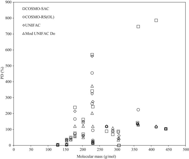
Correlation of model percentage deviations with molecular mass of solute.

Fig. 3.

Correlation of model percentage deviations with van der Waals area parameter (q₁) in benzene as a solvent.

Fig. 4.

Correlation of model percentage deviations with number of different functional groups present in solute for benzene as a solvent.

The NRTL-SAC model was applied to a subset of the dataset considered here. Comparisons are only made to experimental data, as the model is semi-correlative and would not offer a fair comparison to the purely predictive models discussed above. In order to apply the NRTL-SAC model to solubility predictions, the segment area parameters (X,Y+ ,Y− and Z) must be known for the solutes and solvents considered. If these parameters are not available in the literature, they can be regressed from solubility data via the calculation of the activity coefficient, and using pure component property data. Some of the NRTL-SAC model parameters for the solutes were not available in the literature, and were therefore determined by the regression of the solubility data provided in Table S1. These new parameters are available in Table 5, along with literature sources where available.

Table 5.

Calculated segment area parameters for NRTL-SAC.

Solute	This work				Literaturea
	X	Y+	Y−	Z	X	Y+	Y−	Z
Betulin	0.0441	0.0743	0.0189	0.0024	–	–	–	–
Diosgenin	0.1651	0.0112	0.1696	0.0183	–	–	–	–
Mestanolone	0.3224	1.1220	0.7231	0.1953	–	–	–	–
Hydrocortisone	0.4130	1.3020	0.9420	0.7110	0.4010	1.2480	0.9700	1.2480
Estrone	0.4822	1.4240	0.710	0.1973	0.4990	1.5210	0.6790	0.1960
Prednisolone	0.3945	1.1039	1.8975	0.3290	–	–	–	–
Testosterone	1.041	0.2290	0.5460	0.7010	1.0510	0.2330	0.7710	0.6690

^aTaken from Chen and Song [6].

After the application of the NRTL-SAC model, solubility predictions were performed using the new segment area parameters, and solvent parameters, provided by Chen and Song [6], as shown in Fig. 5. The results reveal that the NTRL-SAC model generally does not exhibit any tendency to over-, or underpredict, the experimental solubility. Again, the predictive capability of the model is a qualitative representation, in most cases, of the systems of steroidal APIs that were tested. This is a significant deficiency, as the model is semi-correlative as four component specific model parameters are required for application.

Fig. 5.

Comparison of the natural logarithms of experimental and model calculated solubility composition (x₁) with the NRTL-SAC model.

In Fig. 6 a decision tree is presented to assist in the selection of an appropriate model and assumption for ${\Delta }_{fus}{C}_{pi}$ depending on the solute and solvent class.

Fig. 6.

Decision tree for predictive model selection and ${\Delta }_{fus}{C}_{pi}$ assumption.

5. Conclusion

Where model parameters were available in the literature, solubility predictions were carried out, using various predictive models, for the polycyclic steroidal and triterpene solutes considered in this work.

It was found that the modified UNIFAC (Dortmund) model provided a superior solubility prediction, when benzene as a solvent was considered. The original UNIFAC model provided a superior solubility prediction in aqueous systems. The heat capacity changes of fusion were found to be solvent dependent; and hence, ideal solubility could not be assumed.

A degree of correlation was found between molecular mass and van der Waals surface area, and heat capacity changes of fusion. Generally, the UNIFAC-based, COSMO-based models tended to underestimate the solubility in the triterpene solutes, while the NRTL-SAC model showed no appreciable under- or overestimating tendencies. However, the original UNIFAC model provided a superior solubility prediction for the triterpene/steroid systems, with no significant effect from the assumptions regarding heat capacity changes upon fusion.

New NRTL-SAC segment area parameters have been determined for some of the solutes considered in this work. This information can be used as a subsidiary guide for the selection of solvents in crystallization process design involving the studied solutes, however experimental results will be required if quantitative data is desired.

Conflicts of interest

The authors declare that there are no conflicts of interest.

Appendix. Supplementary material

The following is the supplementary data to this article:

Table S1

Experimental and calculated solubility for various APIs.

References

- 1.Kolář P., Shen J.W., Tsuboi A., Ishikaw T. Solvent selection for pharmaceuticals. Fluid Phase Equilib. 2002;194–197:771–782. [Google Scholar]
- 2.Fredenslund A., Jones R.L., Prausnitz J.M. Group-contribution estimation of activity coefficients in nonideal liquid mixtures. AIChE J. 1975;21:1086–1099. [Google Scholar]
- 3.Weidlich U., Gmehling J. A modified UNIFAC Model. 1. Prediction of VLE hE and γ∞. Ind Eng Chem Res. 1987;26:1372–1381. [Google Scholar]
- 4.Grensemann H., Gmehling J. Performance of a conductor-like screening model for real solvents model in comparison to classical group contribution methods. Ind Eng Chem Res. 2005;44:1610–1624. [Google Scholar]
- 5.Lin S.-T., Sandler S.I. A priori phase equilibrium prediction from a segment contribution solvation model. Ind Eng Chem Res. 2002;41:899–913. [Google Scholar]
- 6.Chen C.C., Song Y. Solubility modeling with a nonrandom two-liquid segment activity coefficient model. Ind Eng Chem Res. 2004;43:8354–8362. [Google Scholar]
- 7.Gmehling J.G., Anderson T.F., Prausnitz J.M. Solid-liquid equilibria using UNIFAC. Ind Eng Chem Fund. 1978;17:269–273. [Google Scholar]
- 8.Gracin S., Brinck T., Rasmuson Å.C. Prediction of solubility of solid organic compounds in solvents by UNIFAC. Ind Eng Chem Res. 2002;41:5114–5124. [Google Scholar]
- 9.Mota F.L., Queimada A.J., Andreatta A.E., Pinho S.P., Macedo E.A. Calculation of drug-like molecules solubility using predictive activity coefficient models. Fluid Phase Equilib. 2012;322:48–55. [Google Scholar]
- 10.Bouillot B., Teychené S., Biscans B. An evaluation of thermodynamic models for the prediction of drug and drug-like molecule solubility in organic solvents. Fluid Phase Equilib. 2011;309:36–52. [Google Scholar]
- 11.Hahnenkamp I., Graubner G., Gmehling J. Measurement and prediction of solubilities of active pharmaceutical ingredients. Int J Pharm. 2010;388:73–81. doi: 10.1016/j.ijpharm.2009.12.036. [DOI] [PubMed] [Google Scholar]
- 12.Diedrichs A., Gmehling J. Solubility calculation of active pharmaceutical ingredients in alkanes alcohols water and their mixtures using various activity coefficient models. Ind Eng Chem Res. 2011;50:1757–1769. [Google Scholar]
- 13.Schröder B., Santos L.M.N.B.F., Marrucho I.M., Coutinho J.A. Prediction of aqueous solubilities of solid carboxylic acids with COSMO-RS. Fluid Phase Equilib. 2010;289:140–147. [Google Scholar]
- 14.Abildskov J., Gani R., Nielsen M.B., Kolar P., Tsuboi A. 2000. Solvent Selection for Drug Development. 2000 AIChE Annual Meeting Los Angeles CA United States 12/11/ [Google Scholar]
- 15.Mishra D., Yalkowsky S. Solubility of organic compounds in non-aqueous systems: polycyclic aromatic hydrocarbons in benzene. Ind Eng Chem. 1990;29:2278–2283. [Google Scholar]
- 16.Neau S.H., Bhandarkar S.V., Hellmuth E.W. Differential molar heat capacities to test ideal solubility estimations. Pharm Res. 1997;14:601–605. doi: 10.1023/a:1012148910975. [DOI] [PubMed] [Google Scholar]
- 17.Hildebrand H., Scott R.L. Prentice-Hall; New Jersey: 1962. Regular solutions. [Google Scholar]
- 18.Hildebrand J.H., Scott R.L. 3rd ed. Dover; New York: 1964. The solubility of nonelectrolytes. [Google Scholar]
- 19.Bondi A. van der Waals Volumes and Radii. J Phys Chem. 1964;68:441–451. [Google Scholar]
- 20.Klamt A. Conductor-like screening model for real solvents: a new approach to the quantitative calculation of solvation phenomena. J Phys Chem. 1995;99:2224–2235. [Google Scholar]
- 21.Staverman A.J. The entropy of high polymer solutions. Generalization of formulae Rec.l Trav. Chim Pays-Bas. 1950;69:163–174. [Google Scholar]
- 22.Guggenheim E.A. 1952. Mixtures. Oxford: U.K. [Google Scholar]
- 23.Chen C.C., Crafts P.A. Correlation and prediction of drug molecule solubility in mixed solvent systems with the Nonrandom Two-Liquid Segment Activity Coefficient (NRTL-SAC) model. Ind Eng Chem Res. 2006;45:4816–4824. [Google Scholar]
- 24.Chen C.C. A segment-based local composition model for the Gibbs energy of polymer solutions. Fluid Phase Equilib. 1993;83:301–312. [Google Scholar]
- 25.Renon H., Prausnitz J. Local compositions in thermodynamic excess functions for liquid mixtures. AIChE J. 1968;14:135–144. [Google Scholar]
- 26.Flory P.J., Krigbaum W.R. Thermodynamics of high polymer solutions. Ann Rev Phys Chem. 1951;2:383–402. [Google Scholar]
- 27.Huggins M.L. Solutions of long chain compounds. J Chem Phys. 1941;9:440. [Google Scholar]
- 28.Chickos J.S., Acree W.E. Total phase change entropies and enthalpies. An update on fusion enthalpies and their estimation. Thermochim Acta. 2009;495:5–13. [Google Scholar]
- 29.Gracin S., Rasmuson Å.C. Solubility of phenylacetic acid p-hydroxyphenylacetic acid p -aminophenylacetic acid p -hydroxybenzoic acid and ibuprofen in pure solvents. J Chem Eng Data. 2002;47:1379–1383. [Google Scholar]
- 30.Roux M.V., Temprado M., Chickos J.S. Vaporization fusion and sublimation enthalpies of the dicarboxylic acids from C4 to C14 and C16. J Chem Thermo. 2005;37:941–953. [Google Scholar]
- 31.Roux M.V., Temprado M., Jiménez P., Foces-Foces C., Garcıa M.V. 2- and 3-furancarboxylic acids: a comparative study using calorimetry IR spectroscopy and X-ray crystallography. Thermochim Acta. 2004;420:59–66. [Google Scholar]
- 32.Rowley J.R., Wilding W.V., Oscarson J.L., Rowley R.L. Brigham Young University; Provo, UT: 2002. DIADEM, DIPPR Information and Data Evaluation Manager. [Google Scholar]
- 33.Zhao G., Yan W. Solubilities of betulin in chloroform + methanol mixed solvents at T = (278.2 288.2 293.2 298.2 308.2 and 313.2) K. Fluid Phase Equilib. 2008;267:79–82. [Google Scholar]
- 34.Moodley K., Rarey J., Ramjugernath D. Experimental solubility for diosgenin and estriol in various solvents within the temperature range T = (293.2 to 328.2) K. J Chem Thermo. 2017;106:199–207. [Google Scholar]
- 35.Domańska U., Pobudkowska A., Pelczarska A., Winiarska-Tusznio M., Gierycz P. Solubility and pKa of select pharmaceuticals in water ethanol and 1-octanol. J Chem Thermo. 2010;42:1465–1472. [Google Scholar]
- 36.Hagen T.A., Flynn G.L. Solubility of hydrocortisone in organic and aqueous media: evidence for regular solution behavior in apolar solvents. J Pharm Sci. 1983;72:409–414. doi: 10.1002/jps.2600720422. [DOI] [PubMed] [Google Scholar]
- 37.Lide D.R. In: CRC Handbook of Chemistry and Physics. 87th ed. Lide D.R., editor. Taylor and Francis; 2007. [Google Scholar]
- 38.Hill R.A., Kirk D.N., Makin H.L.J., Murphy G.M. In: Dictionary of steroids: chemical data structures and bibliographies. Hill R.A., Makin H.L.J., editors. Chapman & Hall; London: 1991. [Google Scholar]
- 39.Nordström F.L., Rasmuson Å.C. Polymorphism and thermodynamics of m-hydroxybenzoic acid. Eur J Pharm Sci. 2006;28:377–384. doi: 10.1016/j.ejps.2006.04.008. [DOI] [PubMed] [Google Scholar]
- 40.Omar W., Ulrich J. Solid liquid equilibrium metastable zone and nucleation parameters of the oxalic acid−water system. Cryst Growth Des. 2006;6:1927–1930. [Google Scholar]
- 41.Sabbah R., Perez L. Étude thermodynamique des acides phtalique isophtalique et téréphtalique. Can J Chem. 1999;77:1508–1513. [Google Scholar]
- 42.Cai X., Grant D.J., Wiedmann T.S. Analysis of the solubilization of steroids by bile salt micelles. J Pharm Sci. 1997;86:372–377. doi: 10.1021/js9602148. [DOI] [PubMed] [Google Scholar]
- 43.Nordström F.L., Rasmuson Å.C. Solubility and melting properties of salicylic acid. J Chem Eng Data. 2006;51:1668–1671. [Google Scholar]
- 44.Kosal E., Lee C.H., Holder G.D. Solubility of progesterone testosterone and cholesterol in supercritical fluids. J Supercrit Fluids. 1992;5:169–179. [Google Scholar]
- 45.Chacko A., Devi R., Abraham S., Mathew B. A comparison of the oxidizing ability of polystyrene-supported linear and cyclic polyoxyethylene bound permanganates. J Appl Polym Sci. 2005;96:1897–1905. [Google Scholar]
- 46.Dortmund Data Bank (DDB) 2012. DDBST Software and Separation Technology GmbH. [Google Scholar]
- 47.Lin H.M., Nash R.A. An experimental method for determining the Hildebrand solubility parameter of organic nonelectrolytes. J Pharm Sci. 1993;82:1018–1026. doi: 10.1002/jps.2600821001. [DOI] [PubMed] [Google Scholar]
- 48.Gharavi M., James K.C., Sanders L.M. Solubilities of mestanolone, methandienone, methyltestosterone, nandrolone and testosterone in homologous series of alkanes and alkanols. Int J Pharm. 1983;14:333–341. [Google Scholar]
- 49.Ruchelman M.W. Solubility studies of estrone in organic solvents using gas-liquid chromatography. Anal Biochem. 1967;19:98–108. doi: 10.1016/0003-2697(67)90139-x. [DOI] [PubMed] [Google Scholar]
- 50.Budavari S., editor. The Merck Index An Encyclopedia of Chemicals Drugs and Biologicals. 11th ed. Merck & Co.; Rahway New Jersey: 1989. [Google Scholar]
- 51.Martin A., Wu P.L., Adjei A., Mehdizadeh M., James K.C., Metzler C. Extended Hildebrand solubility approach: testosterone and testosterone propionate in binary solvents. J Pharm Sci. 1982;71:1334–1340. doi: 10.1002/jps.2600711207. [DOI] [PubMed] [Google Scholar]
- 52.Yalkowsky S.H., Valvani S.C., Roseman T.J. Solubility and partitioning VI: octanol solubility and octanol-water partition coefficients. J Pharm Sci. 1983;72:866–870. doi: 10.1002/jps.2600720808. [DOI] [PubMed] [Google Scholar]
- 53.Bowen D.B., James K.C., Roberts M. An investigation of the distribution coefficients of some androgen esters using paper chromatography. J Pharm Pharmacol. 1970;22:518–522. doi: 10.1111/j.2042-7158.1970.tb10556.x. [DOI] [PubMed] [Google Scholar]
- 54.Rytting J.H., Braxton B.K., Xia J. Topics in Pharmaceutical Sciences 1989. In: Breimer D.D., Crommelin D.J.A, Midha K.K., editors. Proceedings of the 49th International Congress of Pharmaceutical Sciences of FIP. The Hague; 1989. pp. 447–457. [Google Scholar]
- 55.Chen F.X., Zhao M.R., Liu C.C., Peng F.F., Ren B.Z. Determination and correlation of the solubility for diosgenin in alcohol solvents. J Chem Thermo. 2012;50:1–6. [Google Scholar]
- 56.Cao D., Zhao G., Yan W. Solubilities of betulin in 14 solvents at different temperatures. J Chem Eng Data. 2007;52:1366–1368. [Google Scholar]
- 57.McLaughlin E., Zainal H.A. The solubility behaviour of aromatic hydrocarbons in benzene. J. Chem. Soc. 1959;177:863. [Google Scholar]
- 58.Apelblat A., Manzurola E. Solubility of oxalic, malonic, succinic, adipic, maleic, malic, citric, and tartaric acids in water from 278.15 to 338.15 K. J Chem Thermo. 1987;19:317–320. [Google Scholar]
- 59.Apelblat A., Manzurola E. Solubility of ascorbic, 2-furancarboxylic, glutaric, pimelic, salicylic, and o-phthalic acids in water from 279.15 to 342.15 K and apparent molar volumes of ascorbic glutaric and pimelic acids in water at 298.15 K. J Chem Thermo. 1989;21:1005–1008. [Google Scholar]
- 60.Apelblat A., Manzurola E. Solubilities of L-aspartic, DL-aspartic, DL-glutamic, p-hydroxybenzoic, o-anisic, p-anisic, and itaconic acids in water from T= 278 K to T= 345 K. J Chem Thermo. 1997;29:1527–1533. [Google Scholar]
- 61.Manzurola E., Apelblat A. Solubilities of L-glutamic acid, 3-nitrobenzoic acid, p-toluic acid, calcium-L-lactate, calcium gluconate, magnesium-DL-aspartate, and magnesium-L-lactate in water. J Chem Thermo. 2002;34:1127–1136. [Google Scholar]
- 62.Apelblat A., Manzurola E. Solubility of suberic, azelaic, levulinic, glycolic, and diglycolic acids in water from 278.25 K to 361.35 K. J Chem Thermo. 1990;22:289–292. [Google Scholar]
- 63.Scatchard G. Equilibria in non-electrolyte solutions in relation to the vapor pressures and densities of the components. Chem Rev. 1931;8:321–333. [Google Scholar]
- 64.Hildebrand J.H. Solubility. J Am Chem Soc. 1916;38:1452–1473. [Google Scholar]
- 65.Mu T., Rarey J., Gmehling J. Performance of COSMO-RS with sigma profiles from different model chemistries. Ind Eng Chem Res. 2007;46:6612–6629. [Google Scholar]
Associated Data
This section collects any data citations, data availability statements, or supplementary materials included in this article.
Supplementary Materials