Electron Tomography of Paracrystalline 2D Arrays

Abstract

Paracrystalline arrays possess specific types of disorder that reduce the structural information as well as resolution when spatially averaged over repeating motifs. Electron tomography combined with motif classification and averaging can solve the heterogeneity problem and provide information on the structural elements that give rise to the disorder. This chapter describes procedures that would be used in a typical tomography application to identify and characterize a paracrystalline specimen. Particular emphasis is given to actively contracting insect flight muscle, a specimen with particularly difficult to characterize structural heterogeneity and 2-D paracrystalline arrays of myosin-V, from which a particularly high resolution motif average was obtained. All aspects of the study are described including data collection, merging of micrographs to produce the tomogram, alignment to an invariant structural element, classification and averaging of heterogeneous structures, and reassembly of focused class averages into high signal-to-noise ratio representations of the original raw repeats. Particular emphasis is placed on limitations of the various processes to produce the final class averages.

1. Introduction

Electron tomography (ET) might seem a poor choice of technique for determining the structure of a crystalline specimen. Electron crystallography, is a much more powerful method for obtaining near atomic resolution three-dimensional (3D) images of molecules. However, high resolution crystallography requires well ordered arrays that are ordinarily obtained with difficulty. The more usual condition is arrays that are poorly ordered, which would happen if the molecules are heterogeneous in either conformation or composition or both, in which case the spatially averaged 3D image displays an average of heterogeneous structures. The heterogeneity may reveal aspects of function but is lost unless the source of heterogeneity is first identified and similar structures are grouped before averaging.

ET on the other hand seldom achieves resolutions approaching 2 nm (1) and far more often achieves resolutions <4 nm. Despite its resolution limitation, ET can provide a powerful complementary method when intrinsic disorder is present in a two-dimensional (2D) array (2). The strength of ET is its ability to produce a 3D image of even unique objects and as such can provide 3D images of the individual molecules within a disordered array thus revealing the structural variations lost with spatial averaging.

Paracrystals (para - Greek prefix meaning faulty) are arrays with intrinsic disorder. Many kinds of disorder can make an array paracrystalline, such as mixtures of filaments with different structure, which is the case in insect flight muscle (IFM) (3), poor ordering of homogeneous filaments, which is the case in many actin bundles (4), poor order of an otherwise homogeneous protein, such as arrays of myosin-V (1), or compositional heterogeneity of a well ordered assembly to name just a few. We have applied ET to several of the types of paracrystalline specimens mentioned above. Most of the methods described here were developed initially for studies of IFM but have been applied and modified for broader application to a much wider variety of specimens such as the Env spikes of HIV/SIV viruses (5–7), integrins reconstituted into vesicles (8, 9) and bacterial flagellar motors (10).

We use the term “motif” as a synonym for subvolume because of the repetitive nature of paracrystalline arrays and equate it with the term “single-particle” as used in 3D reconstruction from projections. The structure determination of a paracrystalline specimen by ET would be similar to solving a single particle structure when preferred particle orientation is present. The high density of partially aligned motifs in paracrystals is a significant mitigating factor. Generally, the motifs in paracrystals are heterogeneous, otherwise the array would not be paracrystalline. Single-particle methods are most effective when the variation between particles arises primarily from orientation and are more difficult when heterogeneity in structure is also present. The presence of preferred orientation requires that the object be tilted to obtain 3D data, yet the close apposition of motifs within a paracrystal causes superposition when tilted so that a single particle approach to solving the structure using tilt series images is impractical.

ET largely overcomes these problems but with the qualification that the tomograms, especially of ice embedded specimens have low signal-to-noise (S/N) ratio requiring that averages be obtained if molecular conformations are desired. When ET is applied to active muscle, which arguably lacks discrete structural states in the myosin cross-bridges, reduction in the number of structures as well as an accurate count of the different structures is imperative. Improved resolution, improved S/N ratio, data reduction as well as quantification are goals achievable using the techniques of multivariate data analysis (MDA) (11, 12). However, processing of volume data presents additional challenges including angular alignment over three degrees of freedom and treatment of the missing wedge (or pyramid) that do not occur in 2D image classification.

In this chapter, we will describe approaches that we have found useful in structural work on disordered protein arrays. The chapter covers all aspects of the work from data collection to motif classification and averaging. The software used in these studies includes protomo for tilt series alignment (13, 14), i3 for motif alignment and classification (15). Accessory programs have been written for specific functions and these have been combined into shell scripts to handle more complicated tasks that are commonly performed. Table 1 provides a list of i3 modules and a brief description of their function so that comparable modules in other software packages can be substituted if desired. protomo can be downloaded free at http://www.electrontomography.org/.

Table 1.

i3 Software Modules and Their Functions

Multireference Alignment Scripts
i3init.sh, i3make.sh	Create initial database, reads positions, transformations & missing wedge geometry for data subsets. Select & define alignment set from subsets.
i3align.in	Script template for multireference alignment. Each subset can be aligned concurrently. Calls the i3align executable.
i3totsum.sh	Calculate global average. Calls the i3window executable.
i3msa.sh	Compute eigenvalues/eigenimages for multivariate statistical analysis. Calls the i3window and i3svd executables
i3class.sh	Hierarchical ascendant classification, class averages and dendrograms. Calls i3hac and i3window executables.
i3select.sh, i3selectalign.in	Select class averages, align the selected averages with respect to each other concurrently, based on the script template.
i3selectapply.sh	Applies alignment transformation obtained by aligning class averages to the transformation of the raw subvolume, stored in the database.
Executables that operate on whole data sets
i3dataimport, i3datalist	Imports and exports positions & transformations into/out of the database.
i3window	Extract motifs from raw tomograms based on positions & transformations stored in the database. Produces either image stacks or averages.
i3align	Single or multi-reference alignment.
i3svd	Computes a singular value decomposition of image vectors for multivariate statistical analysis.
i3hac	Hierarchical ascendant classification, based on the results of i3svd.
Executables that operate on images
i3cut	Extracts a window.
i3paste	Inserts an image, overwriting pixels in the target image.
i3mask	Apply masks to real space and Fourier space images.
i3fourier	Fourier transform driver; calls selectable transform algorithms.
i3compute	Perform arithmetic operations with images.
i3project	Compute projection in x, y, or z-direction.
i3resample	Apply a linear transformation to an image.
i3concat	Creates an image stack from individual images.
i3avg	Produces an average and/or variance image from an image stack.
i3montage	Produces a montage of individual images or image stacks.
i3stat	Print image statistics.
i3display	Graphical display program and manual motif picking program.

2. Principles of Electron Tomography

Space limitations do not permit a detailed treatment of the principles of ET. For this, the interested reader is referred to two excellent books on ET (16, 17). Here we will limit the discussion to those aspects of ET that directly affect the visualization of molecules within a paracrystalline specimen. Molecular ET has many characteristics in common with single particle 3D image reconstruction, but differs in several key respects. Data are collected using tilt series, which must be aligned first to produce the tomogram. This is followed by alignment, classification and averaging of motifs to improve the S/N ratio and determine heterogeneity. The treatment of defocus (18, 19) also differs but is not covered here.

Dose fractionation is one of the foundations of ET (20–22). Dose fractionation defines the relationship between the S/N ratio in the individual projections with the S/N ratio in the final tomogram. Simply put, if a tilt series can be recorded and aligned using the same total electron dose as a typical projection, the tilt series has the same statistical significance as that projection. However, the two are not equivalent. The tomogram also has higher contrast than its projection, a quality that can be deceptive as it suggests that motifs in tomograms are “better” than projections of single particles recorded with the same electron dose. In fact they are not better; they have the same statistical significance. Consequently, just as reference bias can lead to a faulty result in single particle reconstruction from noisy images, reference bias can also lead to a faulty result in motif averaging in ET.

3. Tilt Series Data Collection

The collection of the tilt series is the most important aspect of ET. The results obtained by motif averaging and classification will be dependent on the quality of the tomogram that in turn will depend on the quality of the tilt series and the accuracy of the tilt series alignment. Several important factors impact the quality of the tomogram: the tilt increment, the choice of dual axis or single axis tilt series, defocus and radiation damage.

3.1. Fixed Increment or Saxton (cosine) Scheme

Data collection in both electron crystallography as well as ET involve tilting the specimen. The main difference is that in ET, all the images of the tilted specimen come from the same array; no assumption is made that any two arrays are identical. In electron crystallography, each array is assumed to be identical, but oriented variably with respect to the tilt azimuth. Typically in electron crystallography, it is assumed that the highest resolution data on each lattice line in the Fourier transform will be spaced at a distance no greater than the inverse of some multiple, which may be 1, of the crystal thickness. This distance in ET when expressed as an angle is often referred to as the tilt angle increment. The tilt angle increment is tightly correlated with the specimen thickness and the desired resolution. The number of views needed for a desired resolution is generally determined from the formula

$$\text{N}=180°\text{D}/\text{d}$$ (1)

where N is the number of images, D is the specimen diameter and d is the desired resolution (23). An alternative formula makes use of the principle that the Fourier transform of an object changes at a rate that is proportional to the specimen thickness, 1/D, and must be measured at least as frequently at the resolution desired. Thus,

$$\mathrm{\theta }={\text{tan}}^{-1}\left(\text{d}/\text{D}\right)$$ (2)

where θ is the increment between images of the tilt series. Both equations express the intuitive feeling that the thicker the specimen, the more rapidly it changes appearance with tilt angle and that fine features change their appearance more rapidly than do coarse features. Equation (1) is strictly speaking valid for spherical objects or cylindrical objects tilted about their axis; these objects do not change in thickness as the tilt angle increases. Hence, tilt series images can be collected in equally spaced increments. However, generally speaking, electron microscopy specimens such as paracrystals are slabs and thus increase in thickness as the specimen is tilted making equation (2) the more correct form. That the image changes more rapidly as the tilt angle increases can have important consequences if cross correlation is used for the tilt series alignment, a procedure known as marker free alignment. Thus, in our work we emphasize tilt increments determined by the Saxton scheme (24), which decreases the tilt increment by the cosine of the tilt angle exactly in tune with the increase in specimen thickness.

3.2. Single-Axis Versus Dual Axis Tomography

It is intuitively obvious that more data will lead to better feature definition in the final reconstruction. Hence, dual axis tilt series will generally lead to better final reconstructions than single axis tilt series, especially when motif averaging is not anticipated. This fact has to be balanced with other considerations, such as radiation damage and defocus determination. Radiation damage is a serious limitation in ET of frozen hydrated specimens, which will not tolerate excessive electron exposure. Negatively stained and plastic embedded sections appear more forgiving because they don’t disappear with excessive electron exposure, but also are more limited with respect to ultimate resolution. Measurement of defocus in extremely low exposure images, such as are taken in cryoET is very problematic. Thus, the extra images required for a dual axis tomogram may be counterbalanced by the need to measure and correct for defocus to obtain the highest resolution.

In muscle fibrils, the filaments are parallel in a typical thin section. The grid, with its ribbon of sections can easily be positioned on the specimen rod with the filament axis roughly parallel to the tilt axis, which is the optimal orientation for filament visibility. Would this kind of specimen benefit from a dual axis data collection scheme under these circumstances? A single-axis tilt series recorded about the filament axis provides the best rendition of the filament profiles. On the other hand, the cross-bridges connecting the thick and thin filaments are generally oriented perpendicular to the filament axis; an axial orientation is least optimal for their visualization. The most recent report on the structure of cross-bridges visualized in IFM using ET utilized dual axis tilt series and showed the best cross-bridge resolution to date (3). This would suggest that there are some advantages to using dual axis tilt series if they can be conveniently obtained.

Dual-axis tomograms of ice embedded specimens have been obtained (25). However, if motif averages are required to obtain the desired information, and motifs can be obtained over a wide range of orientations within a set of tomograms, then single-axis tomography should be sufficient to obtain an average whose transform samples all of Fourier space or at worst leaves only a missing cone of data. This has been the case with many of the studies that have extracted molecular images from tomograms of frozen hydrated specimens for classification and averaging (1, 10, 26, 27).

Special stages designed for side entry goniometers are available for the collection of dual axis electron tomograms even of ice embedded specimens (28) and some newer electron microscopes such as the FEI Polara and Titan-Krios have built-in dual axis capability. However, when a rotation or “flip-flop” holder is unavailable, extracting the grid, rotating it 90° in the holder and then collecting a second tilt series is a simple solution. Remarkably, this has been done for frozen hydrated specimens and an entire second tilt series collected manually (29). The separate tomograms can be merged into a single tomogram (30, 31) or the two tilt series images merged simultaneously (32). Conical tilting (33) is an alternative to dual axis tilt series for plastic embedded and metal replicas, but not at this time for frozen hydrated specimens.

3.3. Radiation Damage

From the earliest days of cryo-EM, it was realized that ice embedded specimens suffer catastrophic damage (34, 35), later referred to as “bubbling”, when the electron dose exceeded that which completely destroyed the crystalline diffraction (36). Thus, practitioners of cryoET typically try to approach the dose for terminal damage without exceeding it. Negatively stained specimens do not display the same terminal damage effect, but even they suffer from radiation damage (37). Plastic embedded specimens often “appear” more resistant to electron irradiation because of their inherently low resolution. However, even they display radiation damage effects, such as specimen thinning, that are more subtle (38). Progressive change in the thickness of the section during tilt series data collection will degrade the final tomogram. Specimen thinning is most rapid in the early stages of irradiation and after an initial rapid change, the rate becomes much slower and can be minimized using minimal electron exposure methods. However, in the dose range of ~50 e⁻/Ų, about 40% of the typical exposure used to collect a tilt series of ice embedded specimens, there is virtually no shrinkage in the z direction (39).

More recently, Wu et al. (3, 40) repeated a study done in 1999 on isometrically contracting IFM (41) using motif classification and averaging. The new data were recorded automatically using a minimal dose procedure whereas the 1999 data were recorded manually while the specimen was continually irradiated resulting in a high total electron exposure. The recent results using motif averaging resolved the helical array of actin subunits on the thin filament. The same procedures carried out on the 1999 data could not, even though the sections were cut from the same specimen block. This observation suggests that even with plastic embedded specimens, continued electron irradiation will lead to progressive destruction of molecular details of the specimen.

Because of differences in the characteristics of CCD cameras, it is advisable to record an exposure series of frozen hydrated specimens using the conditions that are judged suitable for the type of ET data desired. This involves simply recording images repeatedly of a suitable area of the specimen until “bubbling” is observed. If the specimen is suspended over a hole, bubbling is usually observed first on the surrounding matrix and only later within the hole itself.

4. Missing Wedge

The nature of electron microscope specimens, which are thin slabs of material, means that any tomogram will be missing some views of the specimen and thus the final 3-D image comes from incomplete data. Single-axis tilt series have a missing wedge that is usually not larger than ±30° and usually not smaller than ±20°. This missing wedge can affect motif alignment, which is generally based on cross correlation, thereby requiring special weighting schemes (42). It can also influence motif classification since it can affect the visibility of certain features, especially at low resolution, and therefore bias classification in favor of missing wedge orientation rather than structure. On the other hand, when motifs are obtained from multiple tomograms of paracrystals with different tilt azimuths, an average structure can be produced with only a missing cone of data rather than a missing wedge.

The goal of 3D motif classification is different from the goal of 2D motif classification in single particle reconstruction. Classification of projections in single particle reconstruction is largely used to identify different orientations of ostensibly identical objects. Because ET is usually applied to specimens that are heterogeneous, motif classification in ET is largely used to identify heterogeneity; if there were none, spatial averaging would be more appropriate. The power of 3D motif classification lies in the fact that far more of the Fourier transform of the motif is measured than is missing, so the structure and thus its variability is better defined. Because of the preferred orientation enforced by the array, when motif classification is applied to paracrystals, there will always be some regions of the transform that are missing from each motif and some regions that are held in common among all motifs. Thus, the transform of each motif will usually have in common the central section representing the in-plane projection and varying degrees of overlap of the rest of the transform according to the orientation and size of their missing wedges.

All atoms in the specimen contribute to all Fourier coefficients in the molecular transform. Thus, even with a ±30° missing wedge no specimen feature should be entirely missing from a tomogram. However, at low-resolution where ET is generally applied, the transform of certain low-resolution features may be concentrated in a small region of Fourier space. The two best-known examples are the density profile across a lipid bilayer and the mean radial density distribution of a filament. The membrane profile is a 1D projection of the density onto the normal to the membrane. Tomograms of lipid vesicles or native membranes usually reveal the lipid bilayer only along the lateral edges of the vesicle where the transform of the membrane profile falls within the region of measured data; the bilayer is invisible at the top and bottom (43) where the transform of the membrane profile comes to lie within the missing wedge. Thus, classification of integral membrane proteins can be strongly influenced by their orientation with respect to the missing wedge (15).

Information on the mean radial density distribution of a filament is concentrated in the equator of the Fourier transform, for which the power spectrum has the shape of a disk passing through the origin and oriented perpendicular to the filament axis. When the resolution is so low that the subunits of the filament are not visualized, the filament appears as either a stick (F-actin or intermediate filaments) or a straw (microtubules) and the equator contains all the information about the filament. When the filament equator falls within the missing wedge, which occurs when the filament axis is perpendicular to the tilt axis and the filament lies in the specimen plane, the filament will all but disappear in the tomogram (31). Much of the incentive for dual-axis (30, 31) and conical tilt (33) methods in cellular tomography arises from this effect.

In our IFM work, multiple tomograms are collected from identically oriented sections and thus, the missing wedge orientation is identical over the population of motifs effectively eliminating the missing wedge as a parameter in motif classification. In the other paracrystalline specimens described below, the visibility of the membrane has not been an issue as all have been planar. However, the mean radial density distribution across elongated structures has been found to have an effect (15).

The missing wedge also affects motif averages, particularly if the averages are computed in real space, where the point spread function corresponding to the missing wedge is convoluted over the motif. The missing wedge is defined in Fourier space and can thus be treated explicitly only if averages are computed in Fourier space (44). Averaging in real space effectively down weights amplitudes of measured Fourier coefficients; averaging in Fourier space can avoid this using proper weighting. The i3 software counts the number of actual measurements contributing to each Fourier coefficient therefore accounting explicitly for the missing wedge.

5. Alignment of Tilt Series & Computation of the Tomogram

Alignment of tilt series using gold clusters added as fiducial markers is a popular method and can be done using software packages such as IMOD (45). An alternative method, known as “marker-free” alignment (reviewed in (46)), aligns the tilt series based on intrinsic specimen features and this is the method we use exclusively (2, 13, 14). Marker free alignment works readily with thin specimens such as paracrystalline arrays which have the best potential for providing high resolution of macromolecular assemblies. We have also obtained excellent alignment for several different kinds of ice embedded specimens up to ~200 nm thick (5–7). Thicker specimens are more difficult. A hybrid method proposed by (47) benefits from both techniques: an initial marker based alignment is refined subsequently by marker-free alignment. This speeds up the more time-consuming iterative marker free alignment.

The software implementation for our method of marker free tilt series alignment (protomo) is a Python extension module that can be run from within the SPARX environment (48). It can be downloaded from http://www.electrontomography.org/software/. The steps used in the image processing of a typical specimen (Figure 1) are described below. Steps (3), (4), and (5) are iterated; (4) is optional.

1. Raw images are initially cleaned to remove density gradients and density outliers (hot or cold pixels). They can optionally be binned to reduce the image size and speed up the alignment in the initial stages. Images are low pass filtered to the first zero in the contrast transfer function.

2. The initial alignment of the tilt series starts with the image of the untilted specimen as the reference and progresses successively to higher tilt using the neighboring image at the adjacent lower and higher tilt angle as a reference. For the first alignment the tilt angles from the goniometer and the tilt azimuth obtained from previous tomograms collected at this magnification are used as parameters. Coarse alignment takes only minutes after the last image in the tilt series is collected and is carried out either automatically for the whole tilt series, or manually with a graphical software tool (tomoalign-gui) for problematic images or tilt series.

3. An “area matching” refinement scheme is undertaken in which each member of the tilt series is aligned to a reference obtained by reprojecting a preliminary back-projection. This process also starts with the 0° tilt and proceeds to lower and higher tilt angles while successively including each aligned image in the preliminary map computation.

4. A back-projection map can be calculated at this point to produce a 3D reconstruction. If this is an intermediate step, it is recommended to reduce the size of the map in order to speed up the calculation. The size need not be equal to the area that is used for area matching. This reconstruction can be examined to determine whether the specimen has the features desired. If so, the tomogram is further refined using area matching. A better estimate of the specimen thickness is also obtained from this back-projection and is needed as a parameter for the back-projection weighting algorithm.

5. Geometry fitting takes the alignment parameters obtained from the area matching of each image and performs a least squares fit to obtain a new estimate of the tilt series geometry in an attempt to determine the in-plane rotations of the images, the common tilt axis (tilt azimuth) and the three Euler angles that define the specimen orientation relative to the specimen holder more accurately (Figure 3). Included in the rotation defined by the Euler angles is the deviation of the nominal untilted image from 0°.

Figure 1.

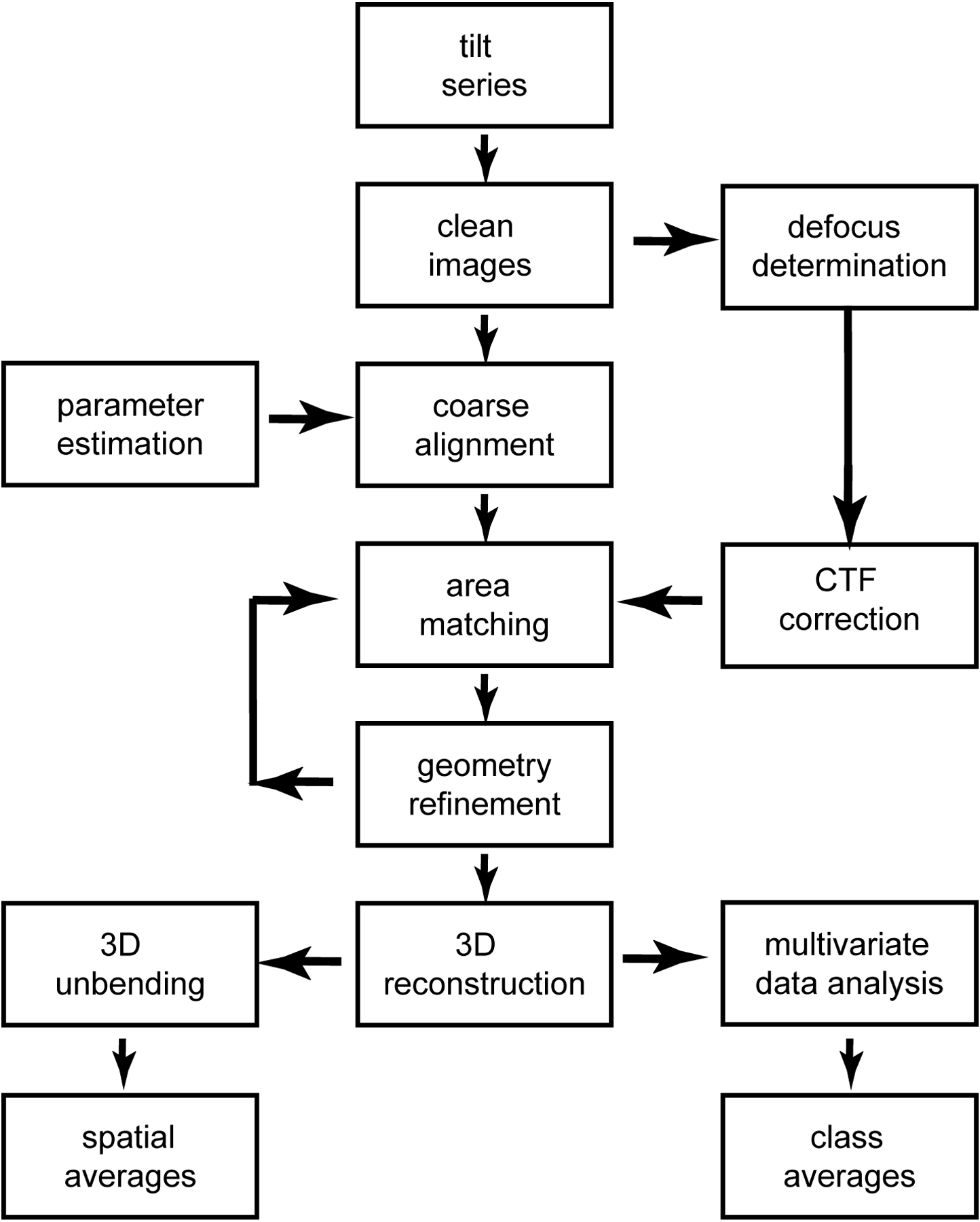
Tomography flowchart. From reference (13).

Figure 3.

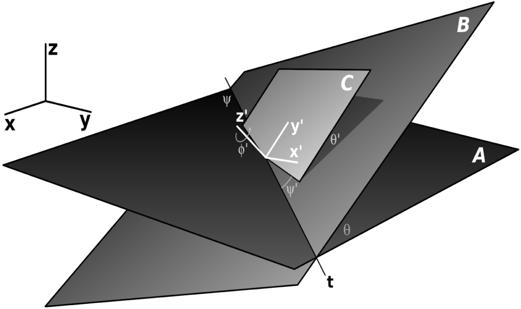
Tilt geometry. (x,y,z): coordinate system fixed with respect to the microscope. z is the optical axis, A (the x-y-plane) is the image plane. (x’,y’,z’): coordinate system fixed with respect to the specimen. The transformation from (x,y,z) to (x’,y’,z’) consists of a tilt about the axis t and angle θ and an additional rotation (ψ’,θ’,φ’) which defines the orientation of the specimen (C) with respect to the specimen holder (B). From reference (13).

Area matching determines four parameters of a linear transformation to match each image to the reference (49). The total transformation is split into two terms, the estimated transformation (which is an input to the area matching) and a correction term. Two parameters of the correction transformation represent the amount of stretch or compression in two orthogonal directions, the other two are the direction of the stretch/compression relative to the corrected and uncorrected image. The stretching/compression factors are plotted as a function of the image number and indicate the progress of the tilt series alignment after each iteration of area matching (Figure 2). The plot of the stretching/compression factors should be flat across the tilt series when alignment and area matching are completed and ideally have a value of 1. In practice, good factors can usually be obtained for the lower tilt angles, while they occasionally deviate more at the high angles. The quality of the alignment is also assessed by the shape and height of the cross-correlation peaks. The peaks should be sharp and strong relative to the local background, but they usually broaden in a direction perpendicular to the tilt axis as the tilt angle increases due to the foreshortening of the projection in the specimen.

Figure 2.

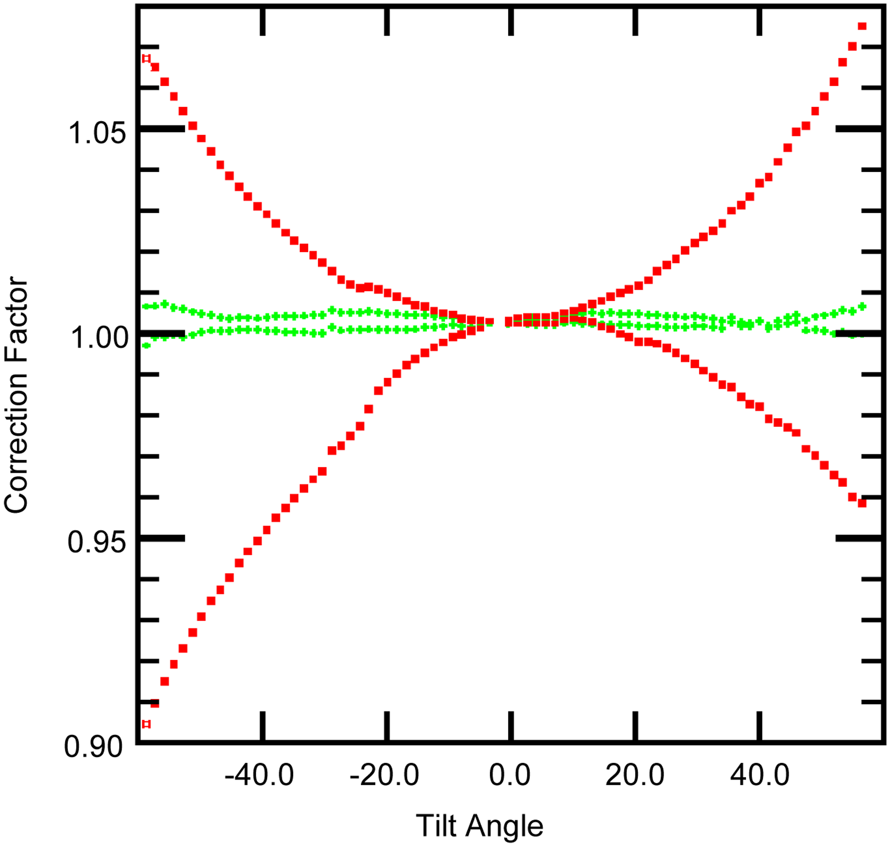
Singular values of the correction matrix after the first iteration (red ■) and after the last iteration (green ♦) for an ice-embedded specimen. Once an accurate estimate of the tilt azimuth has been obtained the singular values usually deviate less than 1% from a value of 1.

protomo uses as the reference image a reprojection of the most recently calculated back-projection. A reprojection is a much better reference, statistically speaking, than any single image in the tilt series and also prevents errors from propagating through the alignment process. Four different cross correlation functions (CCFs) are available in protomo: (1) standard; (2) mutual (50); (3) phases only (51); and (4) phase doubled (52). Phase only CCF, in which amplitudes of all Fourier coefficients are set to 1.0, produces especially sharp correlation peaks even in spatially redundant specimens but requires good alignment before a peak can even be identified. The mutual CCF, which utilizes the square root of the amplitude in the product of the two transforms, is useful when the CCF is periodic or dominated by strong low frequency terms, e.g. muscle. The phase doubled CCF doubles the magnitude of the shift thereby increasing the accuracy.

6. 3D Unbending

One type of heterogeneity that plagues electron crystallography is specimen flatness (53–55). The tomogram contains information on the departure from flatness of a paracrystal since the z coordinate of the motif can be determined thereby providing the potential to correct specimen flatness computationally rather than experimentally. Specimen flatness is particularly likely to affect 2D arrays formed on lipid monolayers, which are most efficiently recovered over holes in reticulated carbon films (56, 57) and whose flatness will be affected by surface tension at the air-water interface. A 3D “unbending” scheme to correct for out-of-plane bending was developed for IFM (58) and used subsequently in a “column averaging” procedure to obtain spatial averages along only the filament axis (41). The approach has not yet been applied to well-ordered 2D crystalline arrays to correct for specimen flatness.

Correction for specimen flatness is also related to the problem of identifying motifs in the paracrystalline array using cross correlation. The software used for 3D unbending is listed in Table 2 along with the functions. The following procedure can be used to calculate a cross correlation map with the goal of correcting a 2D crystalline array for out-of-plane bending:

1. Lattice parameters are determined from a projection of the 3D map, possibly from a slice of the map to reduce noise contributions of the outer sections. Software for conventional 2D array processing such as the MRC package (59) or 2dx (60) can be used for this purpose.

2. An averaged 3D image is calculated by filtering out aperiodic information in the Fourier transform. The filter function is generated using i3createmask by convoluting an array of delta-functions placed at the reciprocal lattice positions with a mask function of rectangular, ellipsoidal, or Gaussian shape, optionally apodized in the rectangular and ellipsoidal case. For arrays of helical filaments, where the transform is continuous in one direction (layer lines), the mask function is extended to the full width of the transform in two dimensions perpendicular to the filament axis.

3. From the averaged 3D image, a reference motif is selected comprising one or more unit cells. Optionally the reference can be generated by other means, in which case step (2) can be skipped. One such possibility would be the use of a raw motif extracted from the tomogram.

4. A cross-correlation map is computed from the tomogram and the generated reference using tomocorr.sh.

5. A peak search is carried out using tomosearch.sh to determine the location of the correlation peak maxima. This is done in two steps. First, a 2-D search determines the x and y coordinates of the maxima from a projection of the correlation map, or better, from a central slice of pre-specified thickness through the map. Then, a 3D search within a small window centered at the previously determined positions and a user-provided z-height locates the actual maxima in the 3D correlation map.

6. A smooth 2D surface is fitted to the measured correlation peaks using tomofit.sh. The fitted spline representation is evaluated on a regular grid of points corresponding to the original sampling points. Points above and below the fitted 2D surface are assumed to lie on lines parallel to the local surface normal in equidistant intervals, corresponding to the lateral sampling distance.

7. The final unbent map is computed by trilinear interpolation of the original map at the points computed in step (6) using tomounbend.sh.

Table 2.

Software Modules for 3-D Unbending

3D unbending Scripts
tomoavg2.sh	spatial averaging
tomomot.sh	create reference motif for cross-correlation
tomocorr.sh	calculate cross-correlation map
tomosearch.sh	determine lattice from observed cross-correlation peaks
tomofit.sh	generate an unbent grid from lattice points by spline fitting
tomounbend.sh	reinterpolate raw map based on the grid
Executables that operate on images
i3createmask	create a periodic mask at reciprocal lattice points for filtering repetitive image structures
i3peaksearch	peak search for lattices in cross-correlation maps
i3unbend3d	spline fitting and reinterpolation

7. Selecting Motifs

Selecting motifs from tomograms of paracrystals can be done by either using cross correlation methods as shown above for 3D unbending or by manual picking. Because the paracrystal is likely to be thin with the motifs positioned within a flat plane, a cross correlation map can usually be calculated from the tomogram projection and peaks fit to obtain a set of x, y coordinates using any of the lattice fitting programs used to analyze 2D crystals (60–63), or the first part of the unbending procedure described above. The z coordinate corresponding to the center of the tomogram will often suffice since the position will be refined later.

Tomograms of paracrystals often contain many separate domains. When this occurs, a CCF is calculated for each domain and a separate lattice fit. Even in IFM, where the motifs usually have at least some similarity, because they are the product of interactions between filaments arranged in parallel, motifs can be selected by fitting a 3-D lattice to a cross correlation map (40).

The use of cross correlation to identify 3D motifs in paracrystals is straight forward, but is not easily applied to randomly oriented motifs, such as envelope spikes on a virus or large individual particles such as ribosomes. The correlation peak height is the measure of similarity between the reference and the “raw” motif, and as such depends on similarity in both orientation and structure as well as the local normalization, and this in turn is affected by the missing wedge (64). Thus, similarities in particle structure and alignment could be offset by missing wedge orientation. This should not present a problem for paracrystals because their preferred orientation within a narrow volume leads to less variability in orientation and thus less effect from the missing wedge and the local normalization.

The alternative approach to motif selection is a manual pick. The image display program, i3display, allows the user to select and mark points in a 3D map or a 2D image (Fig. 4)). i3display is completely general and not specifically designed for paracrystalline arrays. Besides displaying grayscale images, it can thus be used for such diverse activities as picking randomly oriented particles, spikes on envelope viruses and filaments.

Figure 4.

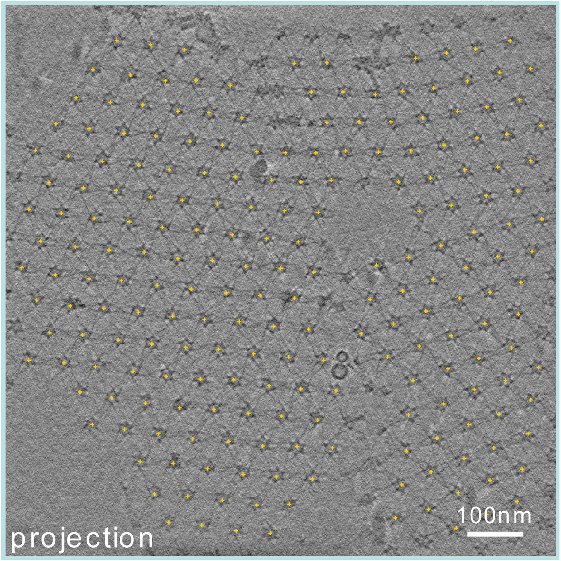
Manual picking using i3display. The image shown is a projection from a tomogram of 2D paracrystalline arrays of myosin-V (1). The centers of so-called “flower motifs” are marked in yellow. Had the image been the actual tomogram, the z-coordinate of these points would be color coded: yellow for points at the same z-level as the currently displayed section, blue for points below and green for points above that level.

If the paracrystal is reasonably flat but too poorly ordered for fitting a CCF, the boxer utility of EMAN (65) is a good alternative for manual picking of motifs from the in-plane projection of the tomogram. A single value for the z coordinate can then be added to the list of particles.

8. Motif Alignment

Before classifying 3D images they must be aligned to an appropriate reference. Invariant functions such as the autocorrelation function that reduce the angular search are not generally available for volumes. Some specialized functions have been constructed, such as an adapted version of the double-autocorrelation method (66), or using spherical harmonics (67). The drawback of the latter is that phase information must be discarded to achieve rotational invariance, and as a consequence these methods, either in 2D or 3D are not as robust and effective as standard cross-correlation alignment.

8.1. Reference Free Alignment

Reference bias must be avoided in order that the result would not depend on the choice of reference. To achieve this, we have adapted a method known as “alignment by classification” (68) to tomographic motifs (15). In this method, raw motifs are not aligned and instead averages obtained in a motif classification step are aligned by multireference alignment and the resulting transformation applied to the class members. For the first alignment step, a simple translational alignment is made to an initial global average. This average generally lacks fine detail. Subsequent alignment and classification will refine fine detail, but only if it appears in the class averages.

Procedures for the initial alignment depend on the orientational degrees of freedom of the motifs, of which the three angular degrees are of primary concern. Application of prior knowledge can greatly reduce the angular search. One example has been described by (15) where the orientation of Env spikes on SIV or HIV virions was computed by fitting an ellipsoidal surface to the manually picked spike positions, under the assumption that the spikes are oriented perpendicular to the surface. The result of the fit defines the geometrical center as well as diameters and orientations of the major axes from which the normal at the position of the spike can be computed. By fitting to an ellipsoid rather than a sphere, deformation of the virion envelope can be approximately accounted for. The program ellipsofit in i3 produces this fit using as input the spike coordinates for individual virions.

Muscle sections are often cut in variable orientations through the filament even when care is used to obtain specific orientations. For example, 80 Å thick transverse sections through the sarcomere are often cut at an angle to the filament axis that can be as large as 20° without appearing to be oblique. In these cases, the following procedure has been found useful to define the initial orientation of the filaments and thus reduce the angular search range:

1. The start and end point of a typical filament, either thick or thin filament will do, is selected using i3display. It is not necessary to select two points for all filaments due to the paracrystalline nature of the muscle.

2. Using i3resample in concert with i3display, the three Euler angles that are needed are determined one by one. These angles can be computed from the two points but it is often essential to verify that the order is applied correctly and for this i3display is used. i3resample utilizes first a rotation about the z-axis, then a rotation around the resulting x-axis and a final rotation about the resulting z-axis.

3. The program i3euler is used to generate a 3 × 3 rotation matrix by giving it the three Euler angles in the same order as determined in (2) above. This matrix is used as the starting orientation for the angular alignment.

The positions of all the motifs within the paracrystal, which can be the center of the filament along the z-axis or the center of a repeating motif, are computed and defined as the rotation center. The centers and rotation matrices are imported from a text file into a database which will be used throughout the motif alignment and classification. The alignment proceeds as follows:

1. Compute a global average of all picked motifs using i3totsum.sh after application of any prior orientation information.

2. Align by translation alone, all of the motifs to the global average using the alignment scripts generated from the template script i3align.in. The generated scripts can be run in parallel.

3. Classify all motifs using i3msa.sh and i3class.sh. For this, a mask must be constructed (see below).

4. Compute class averages.

5. Align all class averages with respect to each other using i3selectalign.in. From among all the multiple orientations for each class average, the alignment parameters are selected from the single class that provides the best overall alignment for all the other classes.

6. Apply the alignment transformations of each class to the respective class members using i3selectapply.sh.

7. Steps 4–6 are applied iteratively until one is satisfied that no further improvement can be obtained. Processing parameters are specified in a parameter file, which is applied to a single cycle “steps 4–6”. Multiple parameter files can be used if parameters change.

No bias is introduced since no arbitrary reference selection takes place. Also, the alignment is carried out with class averages that have a higher S/N ratio, so that it is more robust than a multireference alignment of raw motifs. The number of classes computed in this procedure should be chosen as high as possible, because the goal is to capture as many different spatial orientations as possible in addition to the structural differences. After completion of the alignment procedure, the final classification is based on the expected number of structures.

A problem in the classification of tomographic data is the effect of the missing wedge, which tends to group motifs according to the orientation of the missing wedge rather than structural differences (44). One way to overcome this problem is the use of constrained cross-correlation as a similarity measure for the classification (42). A similar approach based on the signal overlap of a pair of motifs in reciprocal space has been described (67). Additionally, there is also evidence that classification without explicit missing wedge compensation does not necessarily lead to an orientation based grouping of the motifs. A judicious choice of the classification mask can essentially eliminate the effects of the missing wedge. For details see (15).

8.2. Reference Based Alignment

Although it is generally best to use a reference free alignment scheme to avoid reference bias, in some cases, the S/N ratio of the raw tomogram may be sufficiently high and the heterogeneity in the motif structure comparatively low that a reference can be chosen from among the raw motifs with relatively little risk. Liu et al. (69) adopted a reference based alignment scheme to classify motifs from rigor IFM so that actin subunits could be resolved. A similar approach has been used to visualize heterogeneous conformations in myosin and actin (70). In IFM, the least variable structure within each motif is likely to be the actin filament, which is reasonable at the resolutions typical of ET. Based on this assumption, Liu et al. (69) used the following approach.

1. A single actin filament is chosen as a reference from the partly aligned raw motifs selected using a cross correlation map. This reference should have the features that you want enhanced after alignment, such as the staggered arrangement of actin subunits along the filament axis.

2. All the raw motifs are aligned to this reference using a small angular search within a cone of 4° half width about the filament axis.

3. This is followed by several cycles of MDA, using a mask that selects the actin filament, followed by multireference alignment.

4. The process is continued iteratively until the global average reveals the actin subunit structure along the filament.

The procedure is not guaranteed to resolve the actin subunits since that is also a function of preservation and staining.

9. Multivariate Data Analysis and Classification

Improvements in S/N ratio require averaging but this needs to be done within the context of identifying self-similar motifs so that S/N improvement is not achieved at the expense of the structural variation which may be at the heart of the investigation. Motif classification is the solution to this dilemma. Several classification schemes have been used in 2D image classification, among them K-means and hierarchical ascendant methods (HAC), e.g. (71) and Self Organizing Maps (SOM) (72). The classification of heterogeneous cross-bridge motifs in IFM have largely used hierarchical ascendant methods (73) but self organizing maps have proven effective for this use because all motifs have the same missing wedge orientation. K-means classification has been applied to cluster 3D motifs of negatively stained integrins (74). More recently, maximum likelihood approaches have also been investigated (75).

In addition to improvement in S/N ratio, motif averaging can reduce the need for dual axis tilt series as long as the motifs can be obtained over the largest possible range of tilt azimuth. Whatever method is used for classification one must be cognizant of the potential for missing wedge bias. Dual axis tilt series reduce the missing wedge bias and perhaps the need for specialized classification algorithms, though it may not eliminate the problem.

9.1. Mask Construction

In motif classification using MDA, a Boolean mask is computed which defines the voxels that will be used in the classification. The mask is thus a critical component of the procedure. In alignment by classification, it is not necessary to use a single mask for the entire procedure. The mask can be varied throughout the procedure from a very simple one such as a sphere or a cylinder, to a more complex mask derived from the variance map of the global average or from the merged class averages.

Conceptually, volume masks are constructed the same way as projection masks but are somewhat complicated by the added dimension. One method (76) suggests computing a global average, thresholding the average, low-pass filtering, and thresholding again to produce the final Boolean mask. A variance map of the global average is a useful alternative and tends to concentrate the classification on the most variable regions. Masks based on the variance map have been used several times in motif classification (4, 40). Masks can also be computed from the variance maps of the individual class averages using the logical “OR” operation (66). The variance map approach will not be particularly useful until at least some partial alignment has been achieved and the variance map has some structure.

9.2. Number of Classes to Compute

The problem of motif classification particularly in contracting muscle is not one of binning a finite number of discrete states, but rather one of binning a continuum of varying structures. The problem begs the question of what is the most suitable number of bins. S/N improvement and recovery of structure variability are conflicting goals; S/N improvement is achieved by computing the smallest number of classes but recovery of structure variability is achieved by computing the largest reasonable number of classes. HAC allows different numbers of classes to be computed from a single classification run but without an estimate of the optimal number of different classes needed to retain the image variance. SOMs are an alternative method to estimate the number of classes.

One useful tool in assessing the most correct number of classes to compute is the dendrogram, which is a graph produced during the classification by i3class.sh. The dendrogram shows the relationship between the different classes (Figure 5). If the dendrogram shows a number of classes that are similar, then those classes can be merged into a single class. The example shown comes from a classification of myosin-V motifs (1,15) which have undergone MDA to produce five classes. Class 3 is noticeably different from the other 4 in that the myosin heads are closer together than for the other four classes. Classes 1 and 2, which the dendrogram shows are closely related, are obviously different. This difference will be explained below. Classes 0 and 4, which the dendrogram also shows are closely related, appear different because Class 0 has four times as many members as Class 4.

Figure 5.

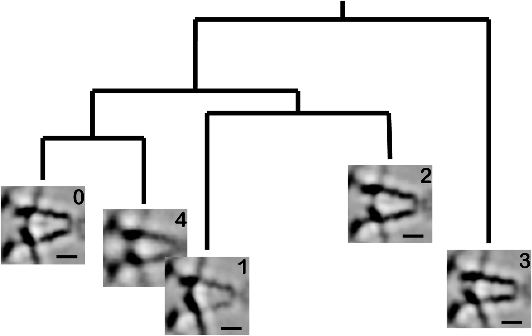
Dendrogram showing the relationship between class averages of myosin-V petal motifs. See Figure 8B legend for explanation of the structural elements. The class number is given in the upper right hand corner. Class 3 is the most isolated class because the myosin heads are more closely apposed than for the other 4 classes, all of which are related at one level. Bar equals 10 nm.

The number of factors (eigenimages) to use in the classification is also not readily defined because classifications optimizing a single feature can be performed using only a limited number of factors. Although the number of factors containing signal can be determined from a plot of the factors after sorting based on their eigenvalues, it is not necessary to use all of these factors for a classification. Factors that may bias the classification in favor of missing wedge orientation can be eliminated from the classification.

9.3. Example 1: Classifying Heterogeneity in Contracting Muscle

Contracting muscle is one challenging example of how image classification and alignment can resolve the highly heterogeneous set of actin-myosin interactions. Muscle has two sets of filaments with different protein compositions and different structures. To get the most information from tomograms of contracting muscle, multiple different sets of classifications would be necessary, each designed specifically for the structure of interest. How this might be accomplished can best be described using the following example. Although the procedure is described using utilities within i3, it was actually performed with a precursor version of i3. Where necessary, the original utility is replaced with the appropriate i3 utility.

Wu et al. (40) described an approach for analysis of highly heterogeneous motifs in contracting muscle that may be applicable for other highly heterogeneous specimens. The approach aligned the set of motifs onto one of the common frames of reference, the actin filament, and utilized the knowledge that the alignment problem was largely one of determining the rotation about the filament axis, which can take on values of either 0° or 180° due to the helical structure of the thin filament. Motifs were defined as 38.7 nm segments of the actin filament centered between successive troponin complexes; successive motifs along each thin filament are rotated 180°. This rotation can be applied to motifs from individual filaments in the initial stages prior to alignment, but entire filaments are also rotated at random by 180° (77) and this has to be determined, but a validity check can be done knowing the rotation of their individual motifs. A multireference alignment scheme was implemented utilizing class averages that showed improved actin subunit detail. Finally, a single reference alignment was applied once the axial rotations were determined in order to place all of the motifs into a single frame of reference, this being necessary to facilitate quasi-atomic model building. Each of the 14 actin subunits in the repeat could then be examined for myosin head binding by a judicious choice of classification mask.

With a common frame of reference, the next problem was to obtain class averages of the myosin heads that were attached to the thin filament. Because the alignment procedure had minimized the variance within the actin filament, the classification mask could exclude those voxels that contained exclusively actin subunits, thereby facilitating a focused classification for specific regions of the motif repeat. A total of 12 different classification masks (Figure 6) were constructed using the following general procedure:

1. Compute the variance map of the global average. The average and variance map are computed using i3avg.

2. Select an appropriate threshold. Usually, this is done by overlaying the global average and variance map in chimera (78) and adjusting the threshold. Chimera can also be used to edit the variance map to eliminate voxels in undesired regions, such as the thick filament backbone.

3. Remove the region occupied by the actin filament. Whole blocks of voxels can be removed using the i3cut utility. Alternatively, a complementary Boolean image can be constructed and the developing mask multiplied sequentially by these Boolean masks to remove entire regions, such as the thick filament backbone or the thin filament core. Images are multiplied together using the i3compute utility. This pair of masks, dubbed primary classification masks, is trimmed axially so that it covers all actin subunits except those to which a troponin complex is bound.

4. The mask is then divided into left and right hand sides using i3cut because these sides will be classified separately.

5. A set of four ellipsoidal masks are constructed covering the vicinal regions of the troponin complex.

6. To provide a cross-check on the primary mask classifications in the region of the lever arms, a key structural parameter of the contracting muscle, the primary classification mask was edited to eliminate the region occupied by the myosin motor domains. These classifications, which are based entirely on the lever arms, were then used to validate the lever arm’s C-terminal positions obtained from the primary mask class averages.

7. A final set of 4 classification masks were constructed by trimming the pair of primary classification masks to cover only pairs of actin subunits outside of the target zone. These masks were used simply for quantifying numbers of attached cross-bridges.

Figure 6.

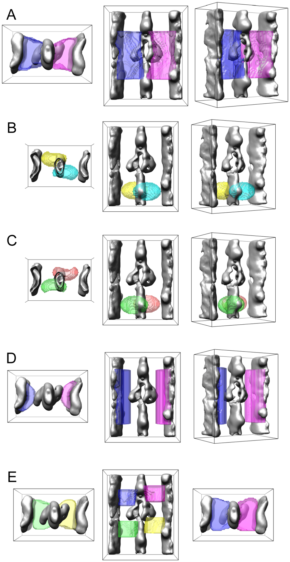
MDA masks. Masks are shown as translucent, colored surfaces superimposed on the global average as a solid gray surface to provide a spatial reference point. (A) Surface display of left (light purple) and right (magenta) primary masks for primary cross-bridge classifications. The actin target zone, where most of the myosin heads bind, is positioned in the middle of the mask. View perspectives from left to right: top view (looking toward Z-line), front view (with the Z-line positioned toward the bottom), and tilted view. (B, C) Surface display of masks specific for troponin bridges. (B) Mask for back-left (yellow) and front-right (cyan) masks. (C) Mask for front-left (green) and back-right (orange) masks. (D) Surface display of masks specific for the myosin lever arms positioned near the thick filament surface. (E) Special mask to identify out-of-target-zone cross-bridges in four separate regions of the repeat. From reference (40).

The presence of numerous focused classifications required a reassembly procedure to make the results interpretable. We define reassembly as the recombination of regions from the different classifications into an improved S/N ratio version of the individual repeats. For the reassembly, Wu et al. (40) utilized six of the focused classifications, the two primary classification masks and the four troponin region masks. The primary classification masks captured cross-bridge structures in and around the target zone, while the troponin bridge masks identified myosin head attachments in and around troponin. The class averages only have meaning for the region within the mask. However, class averages were always computed for the entire motif volume.

Class averages were combined according to their class membership, which is to say that each motif was reassembled from the six class averages to which it contributed (Figure 7). The procedure included the following steps:

1. The two primary mask class averages to which a particular repeat contributed are identified.

2. The left side of the left side class average and the right side of the right side class average were windowed separately using i3cut. Floating and apodizing around the edges is not desirable here and voxels within the rejected region are simply set to zero.

3. The windowed left and right side class averages are then combined using the i3paste utility. If the raw repeat did not contribute to any troponin bridge class averages, the procedure is stopped here. If it contributed to troponin bridge classes, then the next few steps are followed.

4. Usually, there were no more than two troponin bridges in any single motif. However, because troponin bridges are distributed over a comparably large axial range, it was necessary to examine manually the axial extent of the volume that contained the troponin bridge so this procedure could not be automated. Once the axial extent of the troponin bridge was determined, the information could be specified within i3cut to appropriately window out the left side and/or the right side troponin bridge in roughly the same manner as the primary mask class averages.

5. The region of the reassembled primary mask class average that will be replaced with the troponin bridge class average is windowed out using i3cut and the values of the voxels set to zero. The region of the troponin bridge reassembled class average that will be occupied by voxels from the primary mask class average is windowed out and the voxel values set to zero. The two windowed class averages are then added together using the i3paste utility.

6. The final result is low pass filtered to the same resolution as the class averages to remove any seams resulting from the reassembly procedure

Figure 7.

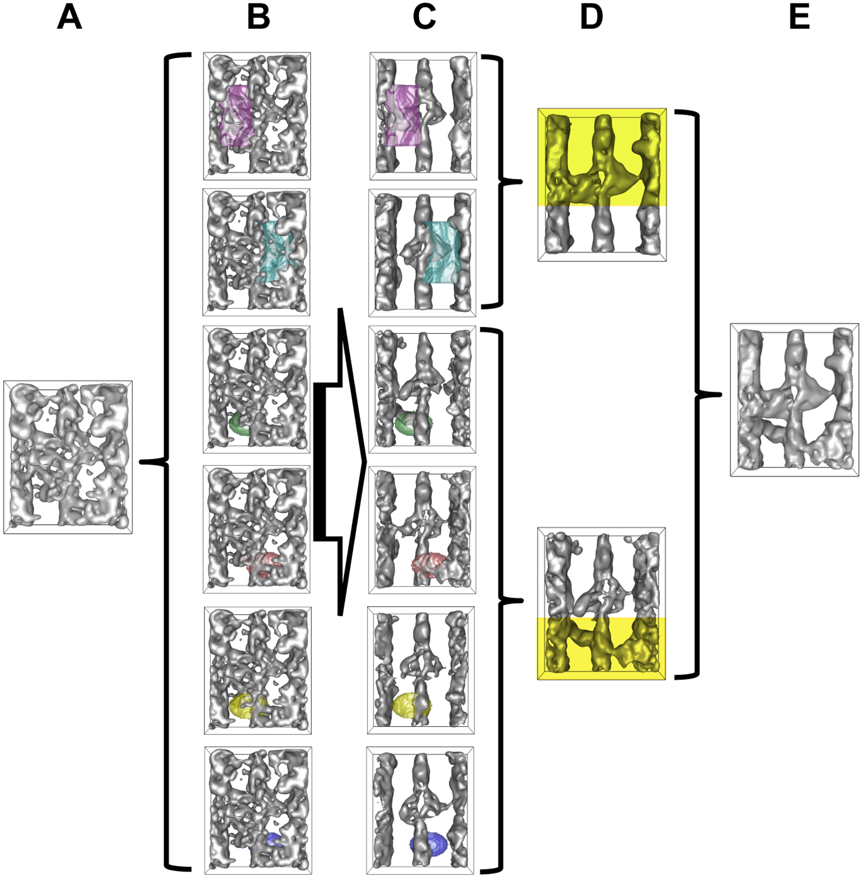
Repeat reassembly. Different masked regions of each raw repeat are subjected to separate MDA and classification using left and right-side primary masks and four Tn region masks. Each classified region is represented by a corresponding class average. The original repeat is represented by a reassembled repeat from all these class averages. From left to right: column A: a raw repeat; column B: six different MDA masks, which are the same as depicted in Figure 5, are applied to this repeat for separate MDA and classification with the mask superimposed; column C: class averages computed for each of the different masked regions of the raw repeat; column D: partially reassembled repeat, the top image combines the class averages from primary left- and right-side classifications and the bottom one combines the class averages from different Tn bridge mask classifications; column E: the whole repeat is reassembled by combining the highlighted portions in column D. Modified from reference (40).

Implicitly, this procedure answers the question of how many classes to compute. If the data set consists of N motifs, then a unique reassembled class average can be obtained for each raw motif if N^1/2 left side and N^1/2 right side class averages are computed.

9.4. Example 2: 2-D arrays of myosin-V

Several different isoforms of the motor protein myosin have been crystallized in 2D on lipid monolayers for structural analysis (1, 79–81). Most of these arrays were well enough ordered that spatial averaging could be used to solve the structure. However, 2D arrays of full length myosin-V proved to be too poorly ordered for spatial averaging (Figure 4). Images of negatively stained arrays show the presence of numerous vacancies within the lattice as well as points where insertions of new rows disrupted the alignment. This kind of disorder provided a perfect opportunity to see whether ET combined with motif averaging and classification could provide a higher resolution result.

The hexagonal unit cell was 653 Å in size and the transform of particularly extensive and well ordered arrays extended to only the 5^th or 6^th order for a resolution of ~ 90 Å (Figure 8A). The final result obtained by motif averaging from defocus corrected electron tomograms of frozen hydrated specimens achieved 25Å by an FSC criterion of 0.5. The cone-flower motif (Figure 8B) showed sufficient detail that the calmodulin light chains could be uniquely positioned and the 15Å wide coiled-coil dimerization domain was clearly seen.

Figure 8.

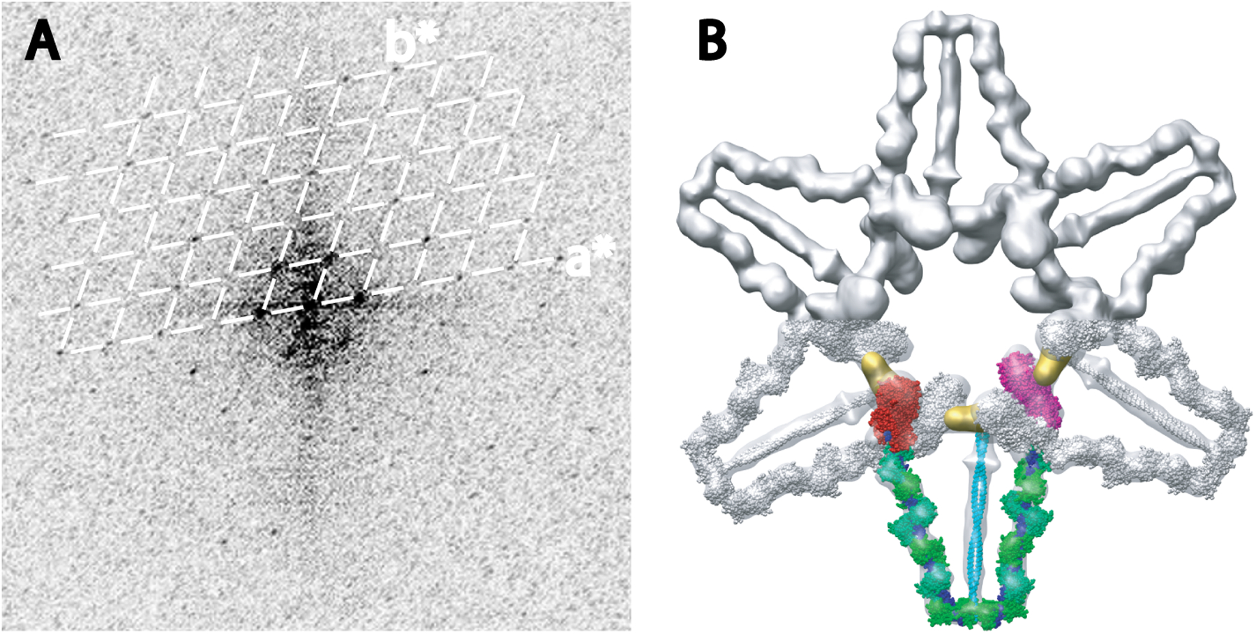
Myosin-V paracrystalline arrays. (A) Power spectrum of a myosin-V array showing the resolution limitation. White lines define the reciprocallattice. Spots extend to about the 5^th order or a resolution of ~90 Å. (B) Molecular arrangement within the “cone-flower” motif. At the top is an opaque surface rendering viewed from the solvent phase onto the lipid monolayer; bottom is a translucent surface view with the myosin-V atomic model rendered in space filling. Color scheme for the bottom molecule: motor domains - red and magenta, light chains – green, heavy chain component of the lever arm - blue, coiled-coil domain - cyan, cargo-binding domain density envelope - yellow, adjacent molecules - gray. Note that the cargo binding domains have swapped binding partners and in the cone-flower motif bind the motor domains of adjacent myosin-V molecules. Panel B from reference (1).

For data collection, a Philips CM300-FEG electron microscope operated at 300 kV. Eight single-axis tilt series were collected at 43,200X magnification. The tilt series were collected using 3.5° cosine rule increments over an angular range of −70° to +70°. Each series consisted of about 60 images. According to Equation 2, and an array thickness of ~100 Å this would be sufficient for a resolution of ~6Å so the tilt series itself was not resolution limiting. The pixel size at the specimen level, 5.56Å, would have been resolution limiting for the tilt increment used, but the final resolution did not reach this limit.

The cumulative electron dose of each tilt series was about 30 e⁻/Ų or about 0.5 e⁻/Ų per image and ~15 e⁻/pixel. At these doses and defoci and with an unstained specimen, the tilt series images themselves show literally nothing except at the highest tilt angles where the array just begins to be visible. However, the tomogram showed very distinctly the hexagonal array of cone-flower motifs in which six myosin-V molecules, the petals, are arranged symmetrically about a 6-fold rotation axis.

Because a CTF correction was anticipated, the data were collected at three different defoci (−5, −8 and −12 μm). Defocus itself was determined with CTFIT (65). Focus gradient correction (18) was applied to each image taken at more than 30° tilt, and a Wiener filter defocus correction was used for images with less than 30° tilt. The defocus-corrected images replaced the low-pass-filtered micrographs for further tilt series refinement.

The first myosin-V structure (1) was obtained before the i3 software was available and utilized both real space averaging without missing wedge compensation, and used a reference based alignment. As part of the development of the i3 software, the data were reanalyzed using reference-free alignment with missing wedge compensation (15). The following protocol is largely based on this reanalysis.

To obtain class averages of the myosin-V petal motif, the following procedure was used.

1. Cone-flower motifs are picked automatically from a cross-correlation map but using the projection of the tomogram. Each coneflower motif has x, y, z dimensions of 200 pixels × 200 pixels × 80 pixels. The z coordinate is initially assigned to be 0.

2. The first alignment cycle used projections rather than volumes to determine the single rotation angle and the x, y displacement.

3. All subsequent cycles of alignment by classification used the volume data and the angular search range over the three Euler angles was limited to a few degrees in order to take into account the wrinkling of the monolayers. Up to 60 class averages were used during the volume alignment step.

4. The final classification produced 20–80 classes but was ultimately reduced to five as the differences between many classes were slight.

The myosin-V study showed a clear effect of the missing wedge (Fig. 9). When carried out using volume data, Classes 1 and 2 had complementary distributions of orientations with respect to the tilt azimuth (Fig. 9A) that produced complementary effects on the density of the lever arm and cargo binding domains. Class 2 had higher density in the lever arm domain and lower density in the cargo binding domain while Class 1 had higher density in the cargo binding domain and lower density in the lever arm. The cargo binding domains and the lever arms are approximately at right angles to each other. The orientations of these classes with respect to the tilt azimuth were such that the lever arms of one were parallel to the tilt azimuth and for the other perpendicular to the tilt azimuth with just the opposite arrangement for the cargo binding domain. This seems to be largely an effect on the average density of the lever arm and cargo binding domain, which have similar shapes overall and in the dendrogram (Figure 5) showed a closer relationship to each other than to the other three classes. In other words, the missing wedge bias in the classification did not lead to a motif with a different overall shape.

Figure 9.

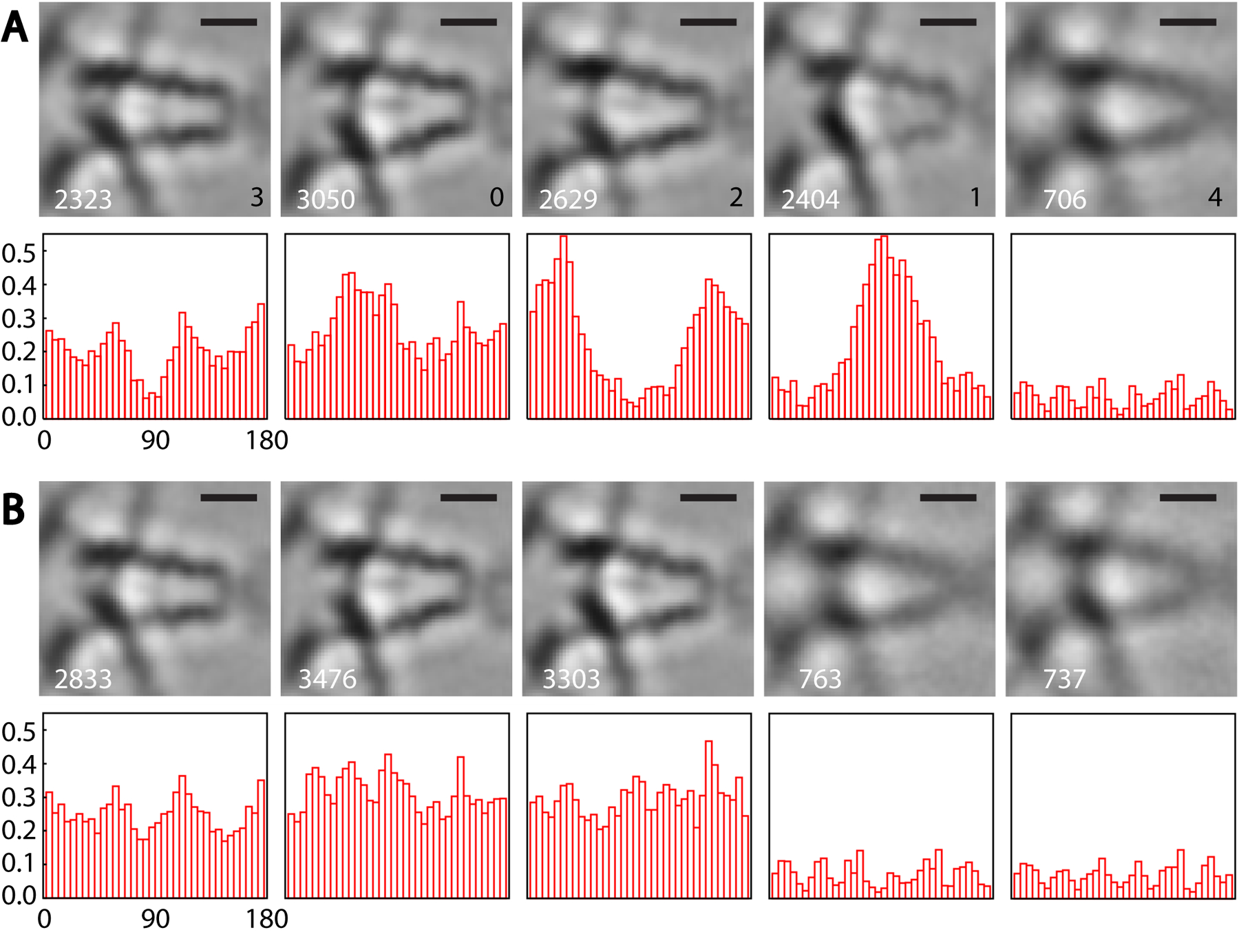
Classification of myosin V petal motifs. See Figure 8B legend for explanation of the structural elements. Bar equals 10 nm. (A) Here the classification was carried out using aligned motifs to produce five classes (0–4, black numbers in the lower right hand corner). The number of motifs (white lettering) contributing to the class averages is given at the bottom left. The bottom row shows histograms of the tilt axis directions with respect to the petal motif with each bin representing the fraction of the total number of motifs that fall within a particular angle range. Note the complementarity of the angular distribution for classes 1 and 2. The complementarity is reflected in the density of the lever arms and the density attributable to the cargo binding domain. (B) Here the classification was carried out with projections of the motifs instead of the motifs themselves. Note that when using the projections the angular bias found for the volumes disappears. Modified from reference (15).

This is exactly the missing wedge effect described above on elongated structures such as filaments. How can this be avoided? With paracrystals, it is quite likely that the motifs will have a limited range of orientations with respect to the optical axis of the microscope so that the projection of the motif can be used in place of the motif itself. When this is done, the classification does not show a missing wedge bias while at the same time, producing averages with the same kind of shape variation (Fig. 9B).

10. Future Prospects

One of the main attractions of molecular ET is the opportunity it provides to look at a molecule’s structure in situ or in vivo and compare it to the structure when removed from its original context. One of the most obvious applications here is the structure of enveloped viruses for which this method has found multiple applications (5, 27, 82–85) but it is also being used to visualize molecular complexes in situ that simply cannot be isolated. The bacterial flagellar motor is one such complex whose details are now being revealed in situ (10, 86, 87). ET also provides a means by which to study a molecular structure in a difficult-to-trap state, such as when it is generating tension in a contracting muscle. It also provides a means to visualize molecules in 3D in states or complexes that are very difficult to isolate with sufficient homogeneity for single particle reconstruction.

These applications all require that the heterogeneity inherent in visualization in situ be treated adequately. MDA as described here is but one approach to classifying heterogeneity. Other methods have been mentioned and improvements in this area are essential if heterogeneous motifs are to be accurately classified.

Advances in several areas could also improve molecular ET, particularly in instrumentation. Improvements in the quality of tomograms are needed as visualization in context becomes increasingly important. An increase in the number of tilt series images that can be recorded and merged from a single specimen are needed to answer demands for higher resolution and applications to thicker specimens. Because radiation damage provides a fundamental limit, increases in the number of images recorded from a single area require offsetting reductions in the number of electrons per image recorded. Such low exposure images become very difficult to both align to produce the tomogram and to measure the defocus to increase the resolution. Defocus measurement might be solved by improvements in accuracy of tracking during data collection so that the tracking defocus is accurate enough to be applied to the area of interest.

Phase plates (88–90) are one area where the contrast, and therefore S/N ratio in each image can be improved thereby providing a possible offset to a reduction in the number of electrons needed per image and resulting increase in the number of images. Phase plates would also allow reductions in defocus, so-called in-focus phase contrast, potentially removing the need to measure defocus in the tilt series.

As specimen thickness increases under the drive for more in situ imaging, inelastic scattering also increases and zero-loss electrons decrease. One solution to this problem is the use of an energy filter with the acceptance window set at the peak of the inelastic scattering (91). This method, known as most-probable loss imaging produces interpretable tomograms even in the near absence of zero-loss electrons. At some point, constructive use of inelastically scattered electrons is going to be a necessity and this will require a chromatic aberration corrector (92). Few of these improvements in instrumentation are widely available at the moment, but they are available in a few selected laboratories.

References

- 1.Liu J, Taylor DW, Krementsova EB, Trybus KM, and Taylor KA (2006) Three-dimensional structure of the myosin V inhibited state by cryoelectron tomography. Nature 442, 208–211. [DOI] [PubMed] [Google Scholar]
- 2.Taylor KA, Tang J, Cheng Y, and Winkler H (1997) The use of electron tomography for structural analysis of disordered protein arrays. J. Struct. Biol 120, 372–386. [DOI] [PubMed] [Google Scholar]
- 3.Wu S, Liu J, Reedy MC, Tregear RT, Winkler H, Franzini-Armstrong C, et al. (2010) Electron tomography of cryofixed, isometrically contracting insect flight muscle reveals novel actin-myosin interactions. PLoS-ONE 5, e12643. [DOI] [PMC free article] [PubMed] [Google Scholar]
- 4.Hampton CM, Liu J, Taylor DW, DeRosier DJ, and Taylor KA (2008) The 3D structure of villin as an unusual F-Actin crosslinker. Structure 16, 1882–1891. [DOI] [PMC free article] [PubMed] [Google Scholar]
- 5.Zhu P, Liu J, Bess J Jr., Chertova E, Lifson JD, Grise H, et al. (2006) Distribution and three-dimensional structure of AIDS virus envelope spikes. Nature 441, 847–852. [DOI] [PubMed] [Google Scholar]
- 6.Zhu P, Winkler H, Chertova E, Taylor KA, and Roux KH (2008) Cryoelectron tomography of HIV-1 envelope spikes: further evidence for tripod-like legs. PLoS Pathog 4, e1000203. [DOI] [PMC free article] [PubMed] [Google Scholar]
- 7.Hu G, Liu J, Taylor KA, and Roux KH (2011) Structural comparison of HIV-1 envelope spikes with and without the V1/V2 loop. J. Virol 85, 2741–2750. [DOI] [PMC free article] [PubMed] [Google Scholar]
- 8.Ye F, Liu J, Winkler H, and Taylor KA (2008) Integrin alpha IIb beta 3 in a membrane environment remains the same height after Mn2+ activation when observed by cryoelectron tomography. J. Mol. Biol 378, 976–986. [DOI] [PMC free article] [PubMed] [Google Scholar]
- 9.Ye F, Hu G, Taylor D, Ratnikov B, Bobkov AA, McLean MA, et al. (2010) Recreation of the terminal events in physiological integrin activation. J. Cell Biol 188, 157–173. [DOI] [PMC free article] [PubMed] [Google Scholar]
- 10.Liu J, Lin T, Botkin DJ, McCrum E, Winkler H, and Norris SJ (2009) Intact flagellar motor of Borrelia burgdorferi revealed by cryo-electron tomography: evidence for stator ring curvature and rotor/C-ring assembly flexion. J. Bacteriol 191, 5026–5036. [DOI] [PMC free article] [PubMed] [Google Scholar]
- 11.Frank J, and van Heel M (1982) Correspondence analysis of aligned images of biological particles. J. Mol. Biol 161, 134–137. [DOI] [PubMed] [Google Scholar]
- 12.Van Heel M, and Frank J (1981) Use of multivariate statistics in analysing the images of biological macromolecules. Ultramicroscopy 6, 187–194. [DOI] [PubMed] [Google Scholar]
- 13.Winkler H, and Taylor KA (2006) Accurate marker-free alignment with simultaneous geometry determination and reconstruction of tilt series in electron tomography. Ultramicroscopy 106, 240–254. [DOI] [PubMed] [Google Scholar]
- 14.Winkler H (2006) 3D reconstruction and processing of volumetric data in cryo-electron tomography. J. Struct. Biol 157, 126–137. [DOI] [PubMed] [Google Scholar]
- 15.Winkler H, Zhu P, Liu J, Ye F, Roux KH, and Taylor KA (2009) Tomographic subvolume alignment and subvolume classification applied to myosin V and SIV envelope spikes. J. Struct. Biol 165, 64–77. [DOI] [PMC free article] [PubMed] [Google Scholar]
- 16.Frank J, (Ed.) (2006) Electron Tomography - Methods for Three-Dimensional Visualization of Structures in the Cell, 2nd ed., Springer-verlag. [Google Scholar]
- 17.McIntosh JR, (Ed.) (2007) Cellular Electron Microscopy, Vol. 79, Academic Press, San Diego, CA. [Google Scholar]
- 18.Winkler H, and Taylor KA (2003) Focus gradient correction applied to tilt series image data used in electron tomography. J. Struct. Biol 143, 24–32. [DOI] [PubMed] [Google Scholar]
- 19.Fernandez JJ, Li S, and Crowther RA (2006) CTF determination and correction in electron cryotomography. Ultramicroscopy 106, 587–596. [DOI] [PubMed] [Google Scholar]
- 20.Hegerl R, and Hoppe W (1976) Influence of electron noise on three-dimensional image reconstruction. Z. Naturforsch 31a, 1717–1721. [Google Scholar]
- 21.Hoppe W, and Hegerl R (1981) Some remarks concerning the influence of electron noise on 3D reconstruction. Ultramicroscopy 6, 205–206. [Google Scholar]
- 22.McEwen BF, Downing KH, and Glaeser RM (1995) The relevance of dose-fractionation in tomography of radiation-sensitive specimens. Ultramicroscopy 60, 357–373. [DOI] [PubMed] [Google Scholar]
- 23.Crowther RA, Amos LA, Finch JT, De Rosier DJ, and Klug A (1970) Three dimensional reconstructions of spherical viruses by fourier synthesis from electron micrographs. Nature 226, 421–425. [DOI] [PubMed] [Google Scholar]
- 24.Saxton WO, Baumeister W, and Hahn M (1984) Three-dimensional reconstruction of imperfect two-dimensional crystals. Ultramicroscopy 13, 57–70. [DOI] [PubMed] [Google Scholar]
- 25.Nickell S, Hegerl R, Baumeister W, and Rachel R (2003) Pyrodictium cannulae enter the periplasmic space but do not enter the cytoplasm, as revealed by cryo-electron tomography. J. Struct. Biol 141, 34–42. [DOI] [PubMed] [Google Scholar]
- 26.Beck M, Forster F, Ecke M, Plitzko JM, Melchior F, Gerisch G, et al. (2004) Nuclear pore complex structure and dynamics revealed by cryoelectron tomography. Science 306, 1387–1390. [DOI] [PubMed] [Google Scholar]
- 27.Förster F, Medalia O, Zauberman N, Baumeister W, and Fass D (2005) Retrovirus envelope protein complex structure in situ studied by cryo-electron tomography. Proc. Natl. Acad. Sci. U S A 102, 4729–4734. [DOI] [PMC free article] [PubMed] [Google Scholar]
- 28.Iancu CV, Wright ER, Benjamin J, Tivol WF, Dias DP, Murphy GE, et al. (2005) A “flip-flop” rotation stage for routine dual-axis electron cryotomography. J. Struct. Biol 151, 288–297. [DOI] [PubMed] [Google Scholar]
- 29.Cheng Y, Boll W, Kirchhausen T, Harrison SC, and Walz T (2007) Cryo-electron tomography of clathrin-coated vesicles: structural implications for coat assembly. J. Mol. Biol 365, 892–899. [DOI] [PMC free article] [PubMed] [Google Scholar]
- 30.Penczek P, Marko M, Buttle K, and Frank J (1995) Double-tilt electron tomography. Ultramicroscopy 60, 393–410. [DOI] [PubMed] [Google Scholar]
- 31.Mastronarde DN (1997) Dual-axis tomography: an approach with alignment methods that preserve resolution. J. Struct. Biol 120, 343–352. [DOI] [PubMed] [Google Scholar]
- 32.Chen LF, Blanc E, Chapman MS, and Taylor KA (2001) Real space refinement of acto-myosin structures from sectioned muscle. J. Struct. Biol 133, 221–232. [DOI] [PubMed] [Google Scholar]
- 33.Lanzavecchia S, Cantele F, and Bellon PL (2001) Alignment of 3D structures of macromolecular assemblies. Bioinformatics 17, 58–62. [DOI] [PubMed] [Google Scholar]
- 34.Taylor KA, and Glaeser RM (1976) Electron microscopy of frozen hydrated biological specimens. J. Ultrastruct. Res 55, 448–456. [DOI] [PubMed] [Google Scholar]
- 35.Taylor KA, and Glaeser RM (1973) Hydrophilic support films of controlled thickness and composition. Rev. Sci. Instrum 44, 1546–1547. [DOI] [PubMed] [Google Scholar]
- 36.Glaeser RM, and Taylor KA (1978) Radiation damage relative to transmission electron microscopy of biological specimens at low temperature: a review. J. Microsc 112, 127–138. [DOI] [PubMed] [Google Scholar]
- 37.Glaeser RM (1971) Limitations to significant information in biological electron microscopy as a result of radiation damage. J. Ultrastruct. Res 36, 466–482. [DOI] [PubMed] [Google Scholar]
- 38.Luther PK (2006) Sample shrinkage and radiation damage of plastic sections, In Electron Tomography - Methods for Three-Dimensional Visualization of Structures in the Cell (Frank J, Ed.) 2nd ed., pp 17–48, Springer-verlag. [Google Scholar]
- 39.Braunfeld MB, Koster AJ, Sedat JW, and Agard DA (1994) Cryo automated electron tomography: towards high-resolution reconstructions of plastic-embedded structures. J. Microsc 174, 75–84. [DOI] [PubMed] [Google Scholar]
- 40.Wu S, Liu J, Reedy MC, Winkler H, Reedy MK, and Taylor KA (2009) Methods for identifying and averaging variable molecular conformations in tomograms of actively contracting insect flight muscle. J. Struct. Biol 168, 485–502. [DOI] [PMC free article] [PubMed] [Google Scholar]
- 41.Taylor KA, Schmitz H, Reedy MC, Goldman YE, Franzini-Armstrong C, Sasaki H, et al. (1999) Tomographic 3-D reconstruction of quick frozen, Ca2+-activated contracting insect flight muscle. Cell 99, 421–431. [DOI] [PubMed] [Google Scholar]
- 42.Förster F, Pruggnaller S, Seybert A, and Frangakis AS (2008) Classification of cryo-electron sub-tomograms using constrained correlation. J. Struct. Biol 161, 276–286. [DOI] [PubMed] [Google Scholar]
- 43.Dierksen K, Typke D, Hegerl R, Walz J, Sackmann E, and Baumeister W (1995) Three-dimensional structure of lipid vesicles embedded in vitreous ice and investigated by automated electron tomography. Biophys. J 68, 1416–1422. [DOI] [PMC free article] [PubMed] [Google Scholar]
- 44.Walz J, Typke D, Nitsch M, Koster AJ, Hegerl R, and Baumeister W (1997) Electron tomography of single ice-embedded macromolecules: three-dimensional alignment and classification. J. Struct. Biol 120, 387–395. [DOI] [PubMed] [Google Scholar]
- 45.Kremer JR, Mastronarde DN, and McIntosh JR (1996) Computer visualization of three-dimensional image data using IMOD. J. Struct. Biol 116, 71–76. [DOI] [PubMed] [Google Scholar]
- 46.Brandt SS (2006) Markerless alignment in electron tomography, In Electron Tomography - Methods for Three-Dimensional Visualization of Structures in the Cell (Frank J, Ed.) 2nd ed., pp 187–216, Springer-verlag. [Google Scholar]
- 47.Liu J, Wright ER, and Winkler H (2010) 3D visualization of HIV virions by cryoelectron tomography. Methods Enzymol. 483, 267–290. [DOI] [PMC free article] [PubMed] [Google Scholar]
- 48.Hohn M, Tang G, Goodyear G, Baldwin PR, Huang Z, Penczek PA, et al. (2007) SPARX, a new environment for Cryo-EM image processing. J. Struct. Biol 157, 47–55. [DOI] [PubMed] [Google Scholar]
- 49.Amat F, Castano-Diez D, Lawrence A, Moussavi F, Winkler H, and Horowitz M (2010) Alignment of cryo-electron tomography datasets. Methods Enzymol. 482, 343–367. [DOI] [PubMed] [Google Scholar]
- 50.Van Heel M, Schatz M, and Orlova E (1992) Correlation functions revisited. Ultramicroscopy 46, 307–316. [Google Scholar]
- 51.Horner JL, and Gianino PD (1984) Phase only matched filtering. Appl. Optics 23, 812–816. [DOI] [PubMed] [Google Scholar]
- 52.Saxton WO (1994) Accurate alignment of sets of images. J. Microsc 174, 61–68. [Google Scholar]
- 53.Vonck J (2000) Parameters affecting specimen flatness of two-dimensional crystals for electron crystallography. Ultramicroscopy 85, 123–129. [DOI] [PubMed] [Google Scholar]
- 54.Han BG, Wolf SG, Vonck J, and Glaeser RM (1994) Specimen flatness of glucose-embedded biological materials for electron crystallography is affected significantly by the choice of carbon evaporation stock. Ultramicroscopy 55, 1–5. [DOI] [PubMed] [Google Scholar]
- 55.Glaeser RM (1992) Specimen flatness of thin crystalline arrays: influence of the substrate. Ultramicroscopy 46, 33–43. [DOI] [PubMed] [Google Scholar]
- 56.Kubalek EW, Kornberg RD, and Darst SA (1991) Improved transfer of two-dimensional crystals from the air/water interface to specimen support grids for high-resolution analysis by electron microscopy. Ultramicroscopy 35, 295–304. [DOI] [PubMed] [Google Scholar]
- 57.Taylor DW, Kelly DF, Cheng A, and Taylor KA (2007) On the freezing and identification of lipid monolayer 2-D arrays for cryoelectron microscopy. J. Struct. Biol 160, 305–312. [DOI] [PMC free article] [PubMed] [Google Scholar]
- 58.Winkler H, and Taylor KA (1996) Three-dimensional distortion correction applied to tomographic reconstructions of sectioned crystals. Ultramicroscopy 63, 125–132. [DOI] [PubMed] [Google Scholar]
- 59.Crowther RA, Henderson R, and Smith JM (1996) MRC image processing programs. J. Struct. Biol 116, 9–16. [DOI] [PubMed] [Google Scholar]
- 60.Gipson B, Zeng X, Zhang ZY, and Stahlberg H (2007) 2dx--user-friendly image processing for 2D crystals. J. Struct. Biol 157, 64–72. [DOI] [PubMed] [Google Scholar]
- 61.Henderson R, Baldwin JM, Downing KH, Lepault J, and Zemlin F (1986) Structure of purple membrane from halobacterium halobium: recording, measurement and evaluation of electron micrographs at 3.5 Å resolution. Ultramicroscopy 19, 147–178. [Google Scholar]
- 62.Baldwin JM, Henderson R, Beckman E, and Zemlin F (1988) Images of purple membrane at 2.8 Å resolution obtained by cryo-electron microscopy. J. Mol. Biol 202, 585–591. [DOI] [PubMed] [Google Scholar]
- 63.Schmid M, Dargahi R, and Tam M (1993) SPECTRA: a system for processing electron images of crystals. Ultramicroscopy 48, 251–264. [DOI] [PubMed] [Google Scholar]
- 64.Frangakis AS, Bohm J, Forster F, Nickell S, Nicastro D, Typke D, et al. (2002) Identification of macromolecular complexes in cryoelectron tomograms of phantom cells. Proc. Natl. Acad. Sci. U S A 99, 14153–14158. [DOI] [PMC free article] [PubMed] [Google Scholar]
- 65.Ludtke SJ, Baldwin PR, and Chiu W (1999) EMAN: semiautomated software for high-resolution single-particle reconstructions. J. Struct. Biol 128, 82–97. [DOI] [PubMed] [Google Scholar]
- 66.Winkler H, and Taylor KA (1999) Multivariate statistical analysis of three-dimensional cross-bridge motifs in insect flight muscle. Ultramicroscopy 77, 141–152. [Google Scholar]
- 67.Bartesaghi A, Sprechmann P, Liu J, Randall G, Sapiro G, and Subramaniam S (2008) Classification and 3D averaging with missing wedge correction in biological electron tomography. J. Struct. Biol 162, 436–450. [DOI] [PMC free article] [PubMed] [Google Scholar]
- 68.Dube P, Tavares P, Lurz R, and van Heel M (1993) The portal protein of bacteriophage SPP1: a DNA pump with 13-fold symmetry. EMBO J. 12, 1303–1309. [DOI] [PMC free article] [PubMed] [Google Scholar]
- 69.Liu J, Reedy MC, Goldman YE, Franzini-Armstrong C, Sasaki H, Tregear RT, et al. (2004) Electron tomography of fast frozen, stretched rigor fibers reveals elastic distortions in the myosin crossbridges. J. Struct. Biol 147, 268–282. [DOI] [PubMed] [Google Scholar]
- 70.Burgess SA, Walker ML, Thirumurugan K, Trinick J, and Knight PJ (2004) Use of negative stain and single-particle image processing to explore dynamic properties of flexible macromolecules. J. Struct. Biol 147, 247–258. [DOI] [PubMed] [Google Scholar]
- 71.Frank J (1990) Classification of macromolecular assemblies studied as ‘single particles’. Q Rev Biophys 23, 281–329. [DOI] [PubMed] [Google Scholar]
- 72.Pascual-Montano A, Taylor KA, Winkler H, Pascual-Marqui RD, and Carazo JM (2002) Quantitative self-organizing maps for clustering electron tomograms. J. Struct. Biol 138, 114–122. [DOI] [PubMed] [Google Scholar]
- 73.van Heel M (1989) Classification of very large electron microscopical image data sets. Optik 82, 114–126. [Google Scholar]
- 74.Iwasaki K, Mitsuoka K, Fujiyoshi Y, Fujisawa Y, Kikuchi M, Sekiguchi K, and Yamada T (2005) Electron tomography reveals diverse conformations of integrin alphaIIbbeta3 in the active state. J. Struct. Biol 150, 259–267. [DOI] [PubMed] [Google Scholar]
- 75.Stolken M, Beck F, Haller T, Hegerl R, Gutsche I, Carazo JM, et al. (2011) Maximum likelihood based classification of electron tomographic data. J. Struct. Biol 175, 77–85. [DOI] [PubMed] [Google Scholar]
- 76.Frank J (1996) Three-Dimensional Elecron Microscopy of Macromolecular Assemblies, Academic Press, San Diego, CA. [Google Scholar]
- 77.Holmes KC, Tregear RT, and Barrington Leigh J (1980) Interpretation of the low angle X-ray diffraction from insect muscle in rigor. Proc. Roy. Soc. (London) - Series B: Biological 207, 13–33. [Google Scholar]
- 78.Pettersen EF, Goddard TD, Huang CC, Couch GS, Greenblatt DM, Meng EC, and Ferrin TE (2004) UCSF Chimera--a visualization system for exploratory research and analysis. J. Comput. Chem 25, 1605–1612. [DOI] [PubMed] [Google Scholar]
- 79.Jontes JD, and Milligan RA (1997) Three-dimensional structure of Brush Border Myosin-I at approximately 20 A resolution by electron microscopy and image analysis. J. Mol. Biol 266, 331–342. [DOI] [PubMed] [Google Scholar]
- 80.Wendt T, Taylor D, Trybus KM, and Taylor K (2001) Three-dimensional image reconstruction of dephosphorylated smooth muscle heavy meromyosin reveals asymmetry in the interaction between myosin heads and placement of subfragment 2. Proc. Natl. Acad. Sci. U S A 98, 4361–4366. [DOI] [PMC free article] [PubMed] [Google Scholar]
- 81.Liu J, Wendt T, Taylor DW, and Taylor KA (2003) Refined model of the 10S conformation of smooth muscle myosin by cryoEM 3-D image reconstruction. J. Mol. Biol 329, 963–972. [DOI] [PubMed] [Google Scholar]
- 82.Grunewald K, Desai P, Winkler DC, Heymann JB, Belnap DM, Baumeister W, and Steven AC (2003) Three-dimensional structure of herpes simplex virus from cryo-electron tomography. Science 302, 1396–1398. [DOI] [PubMed] [Google Scholar]
- 83.Zanetti G, Briggs JA, Grunewald K, Sattentau QJ, and Fuller SD (2006) Cryo-electron tomographic structure of an immunodeficiency virus envelope complex in situ. PLoS Pathog. 2, e83. [DOI] [PMC free article] [PubMed] [Google Scholar]
- 84.Liu J, Bartesaghi A, Borgnia MJ, Sapiro G, and Subramaniam S (2008) Molecular architecture of native HIV-1 gp120 trimers. Nature 455, 109–113. [DOI] [PMC free article] [PubMed] [Google Scholar]
- 85.Dai W, Jia Q, Bortz E, Shah S, Liu J, Atanasov I, et al. (2008) Unique structures in a tumor herpesvirus revealed by cryo-electron tomography and microscopy. J. Struct. Biol 161, 428–438. [DOI] [PMC free article] [PubMed] [Google Scholar]
- 86.Murphy GE, Leadbetter JR, and Jensen GJ (2006) In situ structure of the complete Treponema primitia flagellar motor. Nature 442, 1062–1064. [DOI] [PubMed] [Google Scholar]
- 87.Kudryashev M, Cyrklaff M, Wallich R, Baumeister W, and Frischknecht F (2010) Distinct in situ structures of the Borrelia flagellar motor. J. Struct. Biol 169, 54–61. [DOI] [PubMed] [Google Scholar]
- 88.Nagayama K, and Danev R (2009) Phase-plate electron microscopy: a novel imaging tool to reveal close-to-life nano-structures. Biophys. Rev 1, 37–42. [DOI] [PMC free article] [PubMed] [Google Scholar]
- 89.Murata K, Liu X, Danev R, Jakana J, Schmid MF, King J, et al. (2010) Zernike phase contrast cryo-electron microscopy and tomography for structure determination at nanometer and subnanometer resolutions. Structure 18, 903–912. [DOI] [PMC free article] [PubMed] [Google Scholar]
- 90.Danev R, Kanamaru S, Marko M, and Nagayama K (2010) Zernike phase contrast cryo-electron tomography. J. Struct. Biol 171, 174–181. [DOI] [PubMed] [Google Scholar]
- 91.Bouwer JC, Mackey MR, Lawrence A, Deerinck TJ, Jones YZ, Terada M, et al. (2004) Automated most-probable loss tomography of thick selectively stained biological specimens with quantitative measurement of resolution improvement. J. Struct. Biol 148, 297–306. [DOI] [PubMed] [Google Scholar]
- 92.Freitag B, Kujawa S, Mul PM, Ringnalda J, and Tiemeijer PC (2005) Breaking the spherical and chromatic aberration barrier in transmission electron microscopy. Ultramicroscopy 102, 209–214. [DOI] [PubMed] [Google Scholar]