

Abstract
Optical coherence tomography (OCT) is susceptible to the coherent noise, which is the speckle noise that deteriorates contrast and the detail structural information of OCT images, thus imposing significant limitations on the diagnostic capability of OCT. In this paper, we propose a novel OCT image denoising method by using an end-to-end deep learning network with a perceptually-sensitive loss function. The method has been validated on OCT images acquired from healthy volunteers’ eyes. The label images for training and evaluating OCT denoising deep learning models are images generated by averaging 50 frames of respective registered B-scans acquired from a region with scans occurring in one direction. The results showed that the new approach can outperform other related denoising methods on the aspects of preserving detail structure information of retinal layers and improving the perceptual metrics in the human visual perception.
1. Introduction
Optical coherence tomography (OCT) imaging is currently considered as an indispensable diagnostic tool in ophthalmology [1–3], dermatology [4,5] and cardiology [6,7]. OCT generates in vivo cross-sectional structural images of anatomical structure with microscopic resolution in real time by detecting the interference signals between the reflected signals from the reference mirror and the backscattering signals from biological tissues [8]. As a consequence, OCT is susceptible to the coherent noise, which is the speckle noise that imposes significant limitations on its diagnostic capabilities. The noise deteriorates the contrast of OCT images and the detail structural information [9], and is dependent on both the wavelength of the imaging beam and the structural characteristics of the tissues [9]. Furthermore, poor image quality can affect the accuracy of segmentation of retinal layers [10] and the measurements of tissue thickness [11]. To address this problem, a number of denoising algorithms have been proposed [12–15], among which frame averaging methods [14,15] are the most commonly used in practice. Studies have shown that both the contrast and the quality of OCT images can be improved by averaging the registered multi-frame OCT images acquired from a region with scans occurring in one direction [14,15]. Additionally, averaging more frames increase the contrast and image quality [16]. Nevertheless, this type of procedure requires longer scanning time and therefore is difficult to be performed in clinical practice, especially for elderly patients and infants due to that they cannot keep stationary during image acquisition.
Recently, deep learning has enabled promising applications and achieved significant research results in the field of ophthalmological image processing. On fundus photography, deep learning has been applied in segmentation [17], classification [18], and synthesis [19], while on OCT images, it has been applied in segmentation [20], classification [21], and denoising [22–24]. However, the application of deep learning in OCT image denoising is still in the primitive stage [22–24]. An edge-sensitive conditional generative adversarial network (cGAN) has been proposed to denoise OCT images for commercial OCT scanners [22]. Furthermore, a generative adversarial network (GAN) with Wasserstein distance and perceptual similarity has been proposed to enhance the commercial OCT images [23]. Moreover, a convolutional neural network (CNN) has been proposed and achieved good denoising performance [24]. In all these studies, noisy-label image pairs, which were used for training deep learning models, were generated based on multiple volumetric scans with the registration-averaging method. However, in ordinary clinical practice such approach is limited by the scarcity of usable B-scans in acquiring OCT volumes. Besides that, all these studies require a large OCT training data size for training, which would also limit their potential applications.
Considering the significant feature correlation commonly observed in OCT images, such as the fine structures within each retinal layer and the boundary between different layers, denoising methods should be able to remove the noise without losing the structural details and retain realistic human visual perception. To tackle these issues, this paper proposes a new method based on the end-to-end deep learning technology with a perceptually-sensitive loss function to remove speckle noise in OCT images. The method has been validated on OCT images acquired from healthy volunteers’ eyes. The label images for training and evaluating OCT denoising deep learning models are images averaged from 50 frames of registered B-scans acquired from a region with scans occurring in one direction using our custom OCT scanner. Compared to the traditional denoising methods, well-trained deep learning models are able to exploit spatial correlations at multiple levels of resolution using a hierarchical network, and such correlations are very crucial to the denoising capability. Furthermore, the perceptually-sensitive loss function proposed in this paper has the capability of preserving structure information of OCT images, which is also beneficial to noise reduction.
2. Methods
2.1. Noise reduction for OCT images
A typical OCT imaging system includes a light source, an interferometer, and corresponding electronics components, which inherently induces light intensity noise, photonics shot noise, as well as thermal noise from the electronics. The speckle noise of OCT images can be modeled as multiplicative noise [25]. An OCT image with speckle noise can be defined as:
| (1) |
where is the desired noise-free image, and are the speckle noise and the background noise, respectively.
The objective of OCT denoising methods [12,13,25] is to try to recover a noise-free OCT image from the noisy OCT image . A typical OCT denoising model can be defined as:
| (2) |
where denotes a denoised OCT image generated by an estimator of the denoising model .
2.2. Denoising model estimation using convolutional neural networks
Deep learning is currently considered as the most promising and effective denoising method in medical imaging [22–24,26–30]. Aiming at building deep learning models to reduce the noise of OCT images, CNNs were employed to model the estimator . The training of CNNs consists of forward propagation, loss function calculation, and backpropagation. Briefly, the idea is to first input the noisy OCT images to the neural networks; the convolutional layers output the denoised OCT images, after which the perceptually-sensitive loss function is used to calculate the difference between the denoised OCT images and the label OCT images. Consequently, the back-propagation step passes the loss difference back to the convolutional layers to compute the gradient and update layer weights of the neural networks. Such modeling procedure can be considered as a supervise learning, where CNNs are optimized to minimize the difference between a set of noisy images and a set of label images . Realistically speaking, the set of noise-free images is impossible to obtain. In turn, we use an innovative label data generation operation to get a set of label images as the labels. The deep learning model is trained by minimizing the empirical risk
| (3) |
where is the denoising deep learning model and the is the parameters to be trained. Once the optimal hyper-parameters of the CNNs are determined, the model is successfully established, which can be used for denoising OCT images without further training. A schematic description of the denoising pipeline in this study is shown in Fig. 1.
Fig. 1.

Schematic description of the deep learning-based denoising pipeline for OCT images.
2.3. Network architecture
In this paper, we propose a structure of feed-forward CNN with a perceptually-sensitive loss function to denoise OCT images. The network design is shown in Fig. 2. The -layered deep CNN, which was modified from the denoising convolutional neural networks (DnCNN) [31], contains three types of layers. The input and output of the CNN are the set of noisy OCT images and the denoised images , respectively. The first layer consisted 64 filters (size ) that are used to generate 64 feature maps and rectified linear units (ReLU, ). From layers 2 to layer (-1), there are 64 filters with in size (size ). In contrast to the first layer, batch normalization was added between the convolution layer and the ReLU function. In order to avoid overfitting, dropout was added between batch normalization and the ReLU function. For the output layer, a convolution filter of size was used to reconstruct the denoised OCT image.
Fig. 2.

Schematic overview of the neural network architecture in this study.
2.4. The perceptually-sensitive loss function for the denoising neural network
Loss functions are vital in training deep learning models, and affect the effectiveness and accuracy of the neural networks. Medical images always contain strong structural feature correlations and have strong interdependencies, such as intra-layer structure and boundary between layers in OCT images. The structural similarity index (SSIM) [32] is a metric to evaluate image performance in human visual perception, which is sensitive to changes in local structure and contrast of the images in the human visual perception [33]. In addition, multi-scale SSIM (MS-SSIM), by using SSIM as a basis, extends the effort by making multiple SSIM image evaluations at different image scales. Zhao et al. [34] have discovered that the network trained with MS-SSIM + MSE and MS-SSIM + can generate better results compared to the loss or MSE loss in image restoration tasks. In this study, the MS-SSIM was used as the perceptually-sensitive loss function to train denoising neural network for OCT images. The SSIM is presented as follows:
| (4) |
where and are the means and the standard deviations of the denoised image , respectively; and are the means and the standard deviations of the label image , respectively; denotes the cross-covariance between and ; and are small positive values used to avoid numerical instability.
Compared with SSIM, MS-SSIM provides a multiscale measurement of the image, which can be written as:
| (5) |
where is another form of the label image ; , and are the local image information at the level, and is the number of scales.
Therefore, the perceptually-sensitive loss function can be defined as follows:
| (6) |
3. Experimental setup
3.1. Spectral-domain OCT system
For this study, a classical spectral-domain OCT system was used to acquire the OCT B-scan images. The light source was a wideband super luminescent diode with a central wavelength of 845 nm, and a full width at half maximum bandwidth of 45 nm. The scan size was corresponding to with a macular-centered scanning protocol. The axial resolution and lateral resolution were 6 m and 16 m in our custom OCT scanner, respectively.
3.2. Data acquisition and pre-processing
For data acquisition, 47 groups of OCT B-scans were obtained from 47 healthy eyes, using the OCT scanner. The following protocol was used in the acquisition: 50 frames of B-scan OCT images were obtained along the same scanning direction; potential misalignments in tissue structure that occurred due to eye movement between different scans were eliminated by using a non-rigid registration method with the scale-invariant feature transform, which is implemented on MATLAB. Consequently, the registered noisy B-scan images were averaged to generate a label image with minimal speckle noise. Finally, one of the noisy B-scan images was randomly selected to form noisy-label B-scans pairs. The noisy and label images are shown in Fig. 3.
Fig. 3.

Noisy and label images used in the training phase. (A-C) Noisy OCT images; (D-F) the corresponding label images generated by averaging 50 frames of registered B-scans acquired from a region with scans occurring in one direction.
As for preprocessing, the original images were cropped to pixels by a cropping mask whose central point is the same as the original images. Such a cropping rule eliminates the blurred structure on the peripheral parts of the image. The image patch method was adopted to train the proposed neural networks in order to solve the memory drainage problem raised when using the entire images while training.
3.3. Training details
We designed a 10-layers CNN model, and the network was optimized using the Adam algorithm [35]. The mini-batch size was 64, and the pixel size of the image patches being input was . The training epoch was 100 with a milestone at 50; the learning rate was reduced to 1/10 the original when the training epoch reached the milestone. The training method was implemented using Pytorch (https://pytorch.org/) with a NVIDIA GTX Titan Xp GPU.
The dataset includes two parts, noisy B-scan images and B-scan label images . Each B-scan label image in the respective noisy-label image pair was generated by averaging the 50 frames of registered, as acquired B-scan OCT images. The noisy B-scan image in each pair was randomly selected from the 50 frames of B-scan OCT images along the same direction. 37 of the 47 pairs were used as training dataset, while the remaining 10 pairs were used as test dataset.
3.4. Quantitative metrics
Model evaluation, as well as benchmarking with existing models require quantitative metrics. Four popular performance indices were adopted as such metrics, namely, peak signal-to-noise ratio (PSNR), SSIM [32], MS-SSIM [36], and mean squared error (MSE).
The PSNR and MSE are two classical metrics used in quality measurement between the original and the denoised OCT image. In this work, MSE calculates the cumulative error between the denoised images and the label images, whereas PSNR measures the peak error. A small MSE value implies minor error, and a large PSNR implies better quality of the denoised image.
The MSE is defined as:
| (7) |
where, and are the number of rows and columns of the OCT image, respectively.
The PSNR (in dB) is described as:
| (8) |
where is the maximum possible pixel value of the OCT image.
Considering that the medical images contain strong feature correlations and interdependencies, we adopted the SSIM and the MS-SSIM to evaluate performance in the human visual perception and changes in tissue structure between the denoised OCT images and the corresponding label OCT images. The SSIM and MS-SSIM were respectively calculated as Eq. 4 and 5. They both measure the similarity of structural information in two images, where 0 indicates no similarity and 1 indicates total positive similarity. Although the proposed neural network is being trained with a loss function based on SSIM index, the SSIM and MS-SSIM are still objective and popular quantitative metrics in image restoration tasks [33,34].
3.5. Comparative studies
3.5.1. Comparative studies across different loss functions
To investigate the performance of the proposed perceptually-sensitive loss function in this work, we compared three loss functions with the same neural network, including MSE loss function, loss function, the edge loss function and their various combinations. Due to its convexity and differentiability [37], the MSE loss function is widely used for model optimization in many image processing tasks, such as super-resolution, deburring and denoising. However, it suffers from some inherent defects. When the tasks involve image quality restoration, the MSE loss function poorly correlates with image quality as perceived by the human visual perception since it assumes that the impact of the image noise is unrelated to the local features of the image [34]. Besides, the MSE loss function would make the denoised results unnatural and blurry [38].
The MSE loss function is defined as follows:
| (9) |
where and stand for the height and width of the image, respectively.
Another widely used loss function in image processing tasks is the loss function. The loss solves the problem of over-penalizing of incidental large differences [33]. Therefore, the loss can often outperform the MSE loss. The loss function is defined as follows:
| (10) |
As for OCT image denoising, Ma et al. have proposed the use of edge loss function to preserve the edge of OCT layers [22]. The edge loss function calculates the edge similarity between two images, and therefore is sensitive to the edge-related details.
The edge loss function inspired by the edge preservation index is defined as follows:
| (11) |
where is another form of the label image , and represent coordinates in the longitudinal and lateral direction in the B-scan images.
Besides each loss function, intuitively, combinations of the loss functions have been studied as well. In this work, there were eight loss functions being investigated in the Comparative experiments, which are recorded in Table 1. For simplicity, they were divided into three groups, namely, the conventional loss group (Group 1), the edge-aware loss group (Group 2), and the perceptually-sensitive loss group (Group 3). All trained models were tested on the same OCT test dataset. The compound loss functions of perceptually-sensitive are defined as follows:
| (12) |
where and is weighting factor, and the is the loss or MSE loss function. For the perceptually-senstitive loss together with distance, is 1, and the is 0.01. For the perceptually-senstitive loss together with MSE distance, is 1, and the is 0.02.
Table 1. Groups of the loss functions.
| Group Number | Loss Function | ||
|---|---|---|---|
| Group 1 (Conventional) | loss | MSE loss | |
| Group 2 (Edge-aware) | edge loss alone | edge loss together with distance | edge loss together with MSE distance |
| Group 3 (Perceptually-sensitive) | perceptually-sensitive loss alone | the perceptually-sensitive loss together with distance | the perceptually-sensitive loss together with MSE distance |
Similarly, the compound loss functions of edge-aware is defined as follows:
| (13) |
For the edge-aware loss together with distance, the is 1, and the is 0.025. For the edge-aware loss together with MSE distance, the is 0.95, and the is 0.05.
3.5.2. Comparative studies with traditional methods
The superiority of this method over traditional methods such as block-matching 3D (BM3D) [13] and non-local means (NLM) [12], were established through comparative studies on the same dataset. The details and implementation of these methods could be found in their literature. The quantitative metrics elaborated in Section 3.4 were used to evaluate the performance across the algorithms with the same dataset. The of the Gaussian kernel of the BM3D and the NLM is 30 and 15, respectively.
4. Results
The proposed method successfully and effectively denoise the noisy OCT images. As shown in Fig. 4, the contrast between the layers and the background in the denoised images is obviously enhanced, and the background appears homogeneous. In addition, the detailed structure of retinal tissue are successfully preserved. Furthermore, to better evaluate the performance of the proposed method, two comparative studies were conducted. In the first study, we compared the performance across different loss functions; in the second, we assessed the performance achieved by two well-known traditional denoising methods.
Fig. 4.

Noisy OCT images (A-D) and the corresponding denoised OCT images (E-H).
4.1. Comparative studies across different loss functions
The denoised results of different loss functions are shown in Fig. 5. It can be seen that, the background of the denoised images is homogeneous. The results indicate that all the loss functions are beneficial to improve the quality of noisy OCT images, and in turn reduce the inherent speckle noise. The images produced by Group 2 (edge-aware loss) are blurry with a bit distortion, resulting in small changes of the layer boundary. Moreover, the model with the edge loss function alone failed to perform denoising tasks, thus the corresponding results are not presented in Fig. 5. Group 2 presents the most intra-layer inhomogeneity within all three groups, whereas Group 3 presents the best performance by human visual perception. Such denoised images from Group 3 retain edge information of each layer and the contrast between the layers is enhanced. Besides, either perceptually-sensitive loss together with the MSE distance or with the distance, generate better results than the models using or MSE loss alone, as proved in quantitative evaluations. As for quantitative evaluations, the mean and the standard deviation of each quantitative metrics for the denoised results obtained by the eight different loss functions are listed in Table 2.
Fig. 5.

Denoised results of an OCT image processed by different loss functions. (A) original noisy image; (B) loss function; (C) MSE loss function; (D) combination of edge and ; (E) combination of edge and MSE terms; (F) perceptually-sensitive loss function; (G) combination of perceptually-sensitive and ; (H) combination of perceptually-sensitive and MSE.
Table 2. Quantitative evaluation (mean and standard deviation) across different loss functions.
| Group | CNN | PSNR | SSIM | MS-SSIM | MSE |
|---|---|---|---|---|---|
| Original images | 20.40±0.16 | 0.19±0.02 | 0.59±0.01 | 593.05±20.68 | |
| Group 1 | CNN- | 18.76±0.31 | 0.41±0.05 | 0.84±0.01 | 867.71±61.22 |
| CNN-MSE | 18.78±0.31 | 0.42±0.04 | 0.84±0.01 | 864.05±62.57 | |
| Group 2 | CNN-Edge | Bad result | Bad result | Bad result | Bad result |
| CNN-Edge- | 21.87±0.44 | 0.62±0.06 | 0.86±0.01 | 424.44±44.08 | |
| CNN-Edge-MSE | 19.73±0.32 | 0.49±0.04 | 0.81±0.02 | 693.26±51.62 | |
| Group 3 | CNN-SSIM | 26.40±1.06 | 0.71±0.06 | 0.91±0.01 | 152.94±37.84 |
| CNN-SSIM- | 25.85±0.99 | 0.71±0.06 | 0.91±0.01 | 172.98±37.31 | |
| CNN-SSIM-MSE | 26.37±0.93 | 0.71±0.06 | 0.91±0.01 | 153.27±33.00 |
Note that, perceptually-sensitive loss alone (CNN-SSIM) presents the best performance, illustrating the superiority in practical visual quality.
4.2. Comparative studies with two traditional denoising methods
The results in Section 4.1 have revealed that the proposed method has generated better visual results, with clearer layer structure and more homogeneous intensity distribution within the layers and the background region. Therefore, we compared the proposed method with two widely-used denoising approaches, i.e. BM3D and NLM. The quantitative metrics, which are shown in Table 3, were calculated between the denoised results and their corresponding label images. Although the PSNR and MSE of BM3D are superior compared with the other methods, demonstrating BM3D is still a very powerful noise reduction approach, our proposed method outperforms it on the aspect of similarity of structural information (SSIM and MS-SSIM metrics). Such superiority has been confirmed in Fig. 6, where the background regions of denoised results from BM3D and NLM are not homogeneous and some speckle noise is still observed, resulting in poor contrast of OCT images. Other more serious disadvantages, including loss of fine structure within the layers and the blurred boundaries, can also be observed in the figure.
Table 3. Quantitative evaluation (mean and standard deviation) across BM3D, NLM and CNN with the perceptually-sensitive loss function.
| PSNR | SSIM | MS-SSIM | MSE | |
|---|---|---|---|---|
| Noise | 20.40±0.16 | 0.19±0.02 | 0.59±0.01 | 593.05±20.68 |
| NLM | 26.32±0.54 | 0.45±0.02 | 0.80±0.01 | 152.92±17.90 |
| BM3D | 28.63±0.47 | 0.64±0.03 | 0.86±0.01 | 89.63±10.07 |
| CNN-SSIM | 26.40±1.06 | 0.71±0.06 | 0.91±0.01 | 152.94±37.84 |
Fig. 6.

Denoised results of two OCT images using (A, D) BM3D; (B, E) NLM; (C, F) CNN with the perceptually-sensitive loss function.
5. Discussion
Noise reduction is one of the greatest challenges in OCT image processing. The major difficulty of this task is to achieve a proper balance between maximizing the denoising effect and preserving the structural details. Traditional methods are often limited by the trade-off between these two factors. However, data-driven supervised learning methods may offer a new insight in resolving the dilemma. In our proposed method, the OCT denoising problem was treated as a supervised learning task, taking the advantage of custom dataset with improved labels, and the perceptually-sensitive loss function. This method achieved satisfying performance on the OCT denoising task, outperforming the traditional methods in terms of improved visual quality and retaining detailed features of retinal layers. In this study, a modified DnCNN was employed to denoise OCT images, which is the most well-known denoising deep network architecture and widely used in many denoising tasks [31]. On the other hand, we have also investigated some other network architectures, such as cycleGAN [39] and Residual Network (Resnet) [40]. However, according to the preliminary results listed in Table 4, they have not outperformed over the DnCNN.
Table 4. Quantitative evaluation (mean and standard deviation) across three network architectures with the perceptually-sensitive loss function.
| PSNR | SSIM | MS-SSIM | MSE | |
|---|---|---|---|---|
| DnCNN-Perceptually-sensitive loss | 26.40±1.06 | 0.71±0.06 | 0.91±0.01 | 152.94±37.84 |
| CycleGAN-Perceptually-sensitive loss | 22.66±1.84 | 0.60±0.05 | 0.86±0.02 | 377.35±124.25 |
| Resnet-Perceptually-sensitive loss | 21.97±1.95 | 0.59±0.09 | 0.88±0.02 | 451.33±195.65 |
Our approach has been proved to have higher efficacy in generating denoised images of higher quality compared to other denoising methods, such as NLM and BM3D. With reference to human vision, the NLM and BM3D images were blur with fading intra-layer details and layer boundaries. In addition, the background regions of images acquired through NLM and BM3D were not clean and less homogeneous. After quantitative analysis, additional SSIM and MS-SSIM of NLM and BM3D were not as good as the proposed deep learning methods, which is consistent with their visual quality. The better performance may be caused by the effectiveness of the deep learning algorithms, as well as the perceptually-sensitive loss function, which is friendly to human visual perception [33,34]. The improved label image generation method also aided the improvement of the denoising models. As is widely conceded, better labels are important to data-driven methods, such as the deep learning models.
One of the major highlights of this method is the introduction of the perceptually-sensitive loss function. It has been acknowledged that this kind of loss is able to preserve the image features related to the perception of the human visual perception, and has been verified on various other medical imaging denoising tasks [33]. In this work, generic loss functions (MSE and ) and the well-studied loss function (edge-aware loss function) [22] were used to benchmark the superiority of the perceptually-sensitive loss function. As validated by the quantitative metrics as well as the perceptual characteristics, under the condition of other hyperparameters (depth of layers, mini-batch size, learning rate, etc.) being the same, the perceptually-sensitive loss function outperformed the others. But compound loss functions that combine perceptually-sensitive loss function and conventional loss functions ( and MSE loss functions), may perform even worse than using the perceptually-sensitive ones alone. We further investigated the result of different weights of the loss function component of the compound loss functions of perceptually-sensitive. The preliminary results are presented in Fig. 7. The results indicate there is some fine tune required to boost the performance of the synthesized loss function, and this brings about complexity issues to the problem.
Fig. 7.
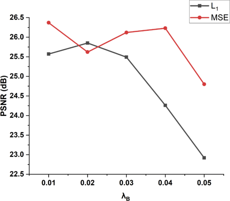
The PSNR values plotted against different weights of the conventional loss functions ( and MSE) in the compound loss function(Eq.12), while was fixed to 1.
Another reason for the success of this method is the innovative label data generation operation. In this study, label images are synthesized from multi-frame scans (50 frames in this study) along the same direction using our custom OCT scanner. The principle of the frame-averaging method indicates that averaging more frames is able to yield a cleaner image. This method generates more accurate labels for training denoising models, and in turn, produces better denoised results. This is consistent with previous findings which suggest that for images with less noise, the denoising models trained by neural networks will likely produce images with less noise, and more accurate textural details [23]. In other words, the performance of image denoising is associated with the label image quality used for training. This labeling method can acquire cleaner label data for training OCT denoising models. In the current study, 37 groups of OCT noisy-label B-scan pairs were used for training the denoising models to produce effectively and successfully denoised results. The data size, compared with related studies, is rather small.
In this study, noisy images and label images, either from healthy eyes or pathologic eyes, are the OCT images from the same region, therefore the noise between both datasets makes up the major portion of the difference. Minimizing such difference is the objective of the denoising models. Based on this fundamental, well-trained denoising models trained from healthy eyes are applicable to pathologic eyes. However, the models may have potential generalization issues when denoise OCT images with pathologic information, since the current training dataset only contains OCT images of healthy volunteers. Future studies should include different pathological OCT images to enhance the generalization capability of the proposed method.
6. Conclusion
In this work, we proposed an effective deep learning network with a perceptually-sensitive loss function to denoise speckle noise from OCT B-scans. This method well preserved information related to detailed structure of retinal layers and improved the perceptual metrics in the human visual perception. We believe the study will facilitate future efforts toward clinical applications.
Acknowledgment
We acknowledge the support of the NVIDIA Corporation with the donation of the Titan Xp GPU used for this research.
Funding
National Natural Science Foundation of China10.13039/501100001809 (81421004, 61875123); National Key Scientific Instrument and Equipment Development Projects of China10.13039/501100012149 (2013YQ030651); Deutscher Akademischer Austauschdienst10.13039/501100001655 (GSSP57145465); Natural Science Foundation of Hebei Province10.13039/501100003787 (H2019201378).
Disclosures
The authors declare no conflicts of interest.
References
- 1.Puliafito C. A., Hee M. R., Lin C. P., Reichel E., Schuman J. S., Duker J. S., Izatt J. A., Swanson E. A., Fujimoto J. G., “Imaging of macular diseases with optical coherence tomography,” Ophthalmology 102(2), 217–229 (1995). 10.1016/S0161-6420(95)31032-9 [DOI] [PubMed] [Google Scholar]
- 2.Drexler W., Morgner U., Ghanta R. K., Kärtner F. X., Schuman J. S., Fujimoto J. G., “Ultrahigh-resolution ophthalmic optical coherence tomography,” Nat. Med. 7(4), 502–507 (2001). 10.1038/86589 [DOI] [PMC free article] [PubMed] [Google Scholar]
- 3.Fujimoto J. G., “Optical coherence tomography for ultrahigh resolution in vivo imaging,” Nat. Biotechnol. 21(11), 1361–1367 (2003). 10.1038/nbt892 [DOI] [PubMed] [Google Scholar]
- 4.Pierce M. C., Strasswimmer J., Park B. H., Cense B., de Boer J. F., “Advances in optical coherence tomography imaging for dermatology,” J. Invest. Dermatol. 123(3), 458–463 (2004). 10.1111/j.0022-202X.2004.23404.x [DOI] [PubMed] [Google Scholar]
- 5.Gambichler T., Moussa G., Sand M., Sand D., Altmeyer P., Hoffmann K., “Applications of optical coherence tomography in dermatology,” J. Dermatol. Sci. 40(2), 85–94 (2005). 10.1016/j.jdermsci.2005.07.006 [DOI] [PubMed] [Google Scholar]
- 6.Kume T., Akasaka T., Kawamoto T., Watanabe N., Toyota E., Neishi Y., Sukmawan R., Sadahira Y., Yoshida K., “Assessment of coronary arterial plaque by optical coherence tomography,” Am. J. Cardiol. 97(8), 1172–1175 (2006). 10.1016/j.amjcard.2005.11.035 [DOI] [PubMed] [Google Scholar]
- 7.Schmitt J., Kolstad D., Petersen C., “Intravascular Optical Coherence Tomography—Opening a Window into Coronary Artery Disease,” Light. Imaging, Inc. Bus. Briefing: Eur. Cardiol. 1(1), 1–5 (2005). 10.15420/ECR.2005.1w [DOI] [Google Scholar]
- 8.Tomlins P. H., Wang R., “Theory, developments and applications of optical coherence tomography,” J. Phys. D: Appl. Phys. 38(15), 2519–2535 (2005). 10.1088/0022-3727/38/15/002 [DOI] [Google Scholar]
- 9.Schmitt J. M., Xiang S., Yung K. M., “Speckle in optical coherence tomography,” J. Biomed. Opt. 4(1), 95–106 (1999). 10.1117/1.429925 [DOI] [PubMed] [Google Scholar]
- 10.Xiang D., Tian H., Yang X., Shi F., Zhu W., Chen H., Chen X., “Automatic segmentation of retinal layer in OCT images with choroidal neovascularization,” IEEE Trans. on Image Process. 27(12), 5880–5891 (2018). 10.1109/TIP.2018.2860255 [DOI] [PubMed] [Google Scholar]
- 11.Devalla S. K., Renukanand P. K., Sreedhar B. K., Subramanian G., Zhang L., Perera S., Mari J.-M., Chin K. S., Tun T. A., Strouthidis N. G., “Drunet: a dilated-residual U-Net deep learning network to segment optic nerve head tissues in optical coherence tomography images,” Biomed. Opt. Express 9(7), 3244–3265 (2018). 10.1364/BOE.9.003244 [DOI] [PMC free article] [PubMed] [Google Scholar]
- 12.Aum J., Kim J.-H., Jeong J., “Effective speckle noise suppression in optical coherence tomography images using nonlocal means denoising filter with double Gaussian anisotropic kernels,” Appl. Opt. 54(13), D43–D50 (2015). 10.1364/AO.54.000D43 [DOI] [Google Scholar]
- 13.Chong B., Zhu Y.-K., “Speckle reduction in optical coherence tomography images of human finger skin by wavelet modified BM3D filter,” Opt. Commun. 291, 461–469 (2013). 10.1016/j.optcom.2012.10.053 [DOI] [Google Scholar]
- 14.Jørgensen T. M., Thomadsen J., Christensen U., Soliman W., Sander B. A., “Enhancing the signal-to-noise ratio in ophthalmic optical coherence tomography by image registration—method and clinical examples,” J. Biomed. Opt. 12(4), 041208 (2007). 10.1117/1.2772879 [DOI] [PubMed] [Google Scholar]
- 15.Alonso-Caneiro D., Read S. A., Collins M. J., “Speckle reduction in optical coherence tomography imaging by affine-motion image registration,” J. Biomed. Opt. 16(11), 116027 (2011). 10.1117/1.3652713 [DOI] [PubMed] [Google Scholar]
- 16.Wu W., Tan O., Pappuru R. R., Duan H., Huang D., “Assessment of frame-averaging algorithms in OCT image analysis,” Ophthalmic Surgery, Lasers Imaging Retin. 44(2), 168–175 (2013). 10.3928/23258160-20130313-09 [DOI] [PMC free article] [PubMed] [Google Scholar]
- 17.Li Z., He Y., Keel S., Meng W., Chang R. T., He M., “Efficacy of a deep learning system for detecting glaucomatous optic neuropathy based on color fundus photographs,” Ophthalmology 125(8), 1199–1206 (2018). 10.1016/j.ophtha.2018.01.023 [DOI] [PubMed] [Google Scholar]
- 18.Gulshan V., Peng L., Coram M., Stumpe M. C., Wu D., Narayanaswamy A., Venugopalan S., Widner K., Madams T., Cuadros J., “Development and validation of a deep learning algorithm for detection of diabetic retinopathy in retinal fundus photographs,” JAMA 316(22), 2402–2410 (2016). 10.1001/jama.2016.17216 [DOI] [PubMed] [Google Scholar]
- 19.Yu Z., Xiang Q., Meng J., Kou C., Ren Q., Lu Y., “Retinal image synthesis from multiple-landmarks input with generative adversarial networks,” Biomed. Eng. Online 18(1), 62 (2019). 10.1186/s12938-019-0682-x [DOI] [PMC free article] [PubMed] [Google Scholar]
- 20.Schlegl T., Waldstein S. M., Bogunovic H., Endstraßer F., Sadeghipour A., Philip A.-M., Podkowinski D., Gerendas B. S., Langs G., Schmidt-Erfurth U., “Fully automated detection and quantification of macular fluid in OCT using deep learning,” Ophthalmology 125(4), 549–558 (2018). 10.1016/j.ophtha.2017.10.031 [DOI] [PubMed] [Google Scholar]
- 21.Karri S. P. K., Chakraborty D., Chatterjee J., “Transfer learning based classification of optical coherence tomography images with diabetic macular edema and dry age-related macular degeneration,” Biomed. Opt. Express 8(2), 579–592 (2017). 10.1364/BOE.8.000579 [DOI] [PMC free article] [PubMed] [Google Scholar]
- 22.Ma Y., Chen X., Zhu W., Cheng X., Xiang D., Shi F., “Speckle noise reduction in optical coherence tomography images based on edge-sensitive cGAN,” Biomed. Opt. Express 9(11), 5129–5146 (2018). 10.1364/BOE.9.005129 [DOI] [PMC free article] [PubMed] [Google Scholar]
- 23.Halupka K. J., Antony B. J., Lee M. H., Lucy K. A., Rai R. S., Ishikawa H., Wollstein G., Schuman J. S., Garnavi R., “Retinal optical coherence tomography image enhancement via deep learning,” Biomed. Opt. Express 9(12), 6205–6221 (2018). 10.1364/BOE.9.006205 [DOI] [PMC free article] [PubMed] [Google Scholar]
- 24.Shi F., Cai N., Gu Y., Hu D., Ma Y., Chen Y., Chen X., “DeSpecNet: a CNN-based method for speckle reduction in retinal optical coherence tomography images,” Phys. Med. Biol. 64(17), 175010 (2019). 10.1088/1361-6560/ab3556 [DOI] [PubMed] [Google Scholar]
- 25.Wang X., Yu X., Liu X., Si C., Chen S., Wang N., Liu L., “A two-step iteration mechanism for speckle reduction in optical coherence tomography,” Biomed. Signal Process. & Control. 43, 86–95 (2018). 10.1016/j.bspc.2018.02.011 [DOI] [Google Scholar]
- 26.Lu Y., Kowarschik M., Huang X., Xia Y., Choi J.-H., Chen S., Hu S., Ren Q., Fahrig R., Hornegger J., Maier A., “A learning-based material decomposition pipeline for multi-energy x-ray imaging,” Med. Phys. 46(2), 689–703 (2019). 10.1002/mp.13317 [DOI] [PubMed] [Google Scholar]
- 27.Liu X., Huang Z., Wang Z., Wen C., Jiang Z., Yu Z., Liu J., Liu G., Huang X., Maier A., Ren Q., Lu Y., “A deep learning based pipeline for optical coherence tomography angiography,” J. Biophotonics 12(10), e201900008 (2019). 10.1002/jbio.201900008 [DOI] [PubMed] [Google Scholar]
- 28.Maier A., Syben C., Lasser T., Riess C., “A gentle introduction to deep learning in medical image processing,” Z. Med. Phys. 29(2), 86–101 (2019). 10.1016/j.zemedi.2018.12.003 [DOI] [PubMed] [Google Scholar]
- 29.Lu Y., Kowarschik M., Huang X., Chen S., Ren Q., Fahrig R., Hornegger J., Maier A., “Material decomposition using ensemble learning for spectral x-ray imaging,” IEEE Trans. Radiat. Plasma Med. Sci. 2(3), 194–204 (2018). 10.1109/TRPMS.2018.2805328 [DOI] [Google Scholar]
- 30.Jiang Z., Yu Z., Feng S., Huang Z., Peng Y., Guo J., Ren Q., Lu Y., “A super-resolution method-based pipeline for fundus fluorescein angiography imaging,” Biomed. Eng. Online 17(1), 125 (2018). 10.1186/s12938-018-0556-7 [DOI] [PMC free article] [PubMed] [Google Scholar]
- 31.Zhang K., Zuo W., Chen Y., Meng D., Zhang L., “Beyond a gaussian denoiser: Residual learning of deep cnn for image denoising,” IEEE Trans. on Image Process. 26(7), 3142–3155 (2017). 10.1109/TIP.2017.2662206 [DOI] [PubMed] [Google Scholar]
- 32.Wang Z., Bovik A. C., Sheikh H. R., Simoncelli E. P., “Image quality assessment: from error visibility to structural similarity,” IEEE Trans. on Image Process. 13(4), 600–612 (2004). 10.1109/TIP.2003.819861 [DOI] [PubMed] [Google Scholar]
- 33.You C., Yang Q., Gjesteby L., Li G., Ju S., Zhang Z., Zhao Z., Zhang Y., Cong W., Wang G., “Structurally-sensitive multi-scale deep neural network for low-dose CT denoising,” IEEE Access 6, 41839–41855 (2018). 10.1109/ACCESS.2018.2858196 [DOI] [PMC free article] [PubMed] [Google Scholar]
- 34.Zhao H., Gallo O., Frosio I., Kautz J., “Loss functions for image restoration with neural networks,” IEEE Trans. Comput. Imaging 3(1), 47–57 (2017). 10.1109/TCI.2016.2644865 [DOI] [Google Scholar]
- 35.Kingma D. P., Ba J., “Adam: A method for stochastic optimization,” Proc. 3rd Int. Conf. on Learn. Represent. (2014).
- 36.Wang Z., Simoncelli E. P., Bovik A. C., “Multiscale structural similarity for image quality assessment,” in The Thrity-Seventh Asilomar Conference on Signals, Systems and Computers, vol. 2 (IEEE, 2003), pp. 1398–1402. [Google Scholar]
- 37.Wang Z., Bovik A. C., “Mean squared error: Love it or leave it? A new look at signal fidelity measures,” IEEE Signal Process. Mag. 26(1), 98–117 (2009). 10.1109/MSP.2008.930649 [DOI] [Google Scholar]
- 38.Chen H., Zhang Y., Kalra M. K., Lin F., Chen Y., Liao P., Zhou J., Wang G., “Low-dose CT with a residual encoder-decoder convolutional neural network,” IEEE Trans. Med. Imaging 36(12), 2524–2535 (2017). 10.1109/TMI.2017.2715284 [DOI] [PMC free article] [PubMed] [Google Scholar]
- 39.Zhu J.-Y., Park T., Isola P., Efros A. A., “Unpaired image-to-image translation using cycle-consistent adversarial networks,” in Proceedings of the IEEE international conference on computer vision, (2017), pp. 2223–2232. [Google Scholar]
- 40.Jifara W., Jiang F., Rho S., Cheng M., Liu S., “Medical image denoising using convolutional neural network: a residual learning approach,” J. Supercomput. 75(2), 704–718 (2019). 10.1007/s11227-017-2080-0 [DOI] [Google Scholar]