Methods for Rapid Mobility Estimation to Support Outbreak Response

Abstract

When pressed for time, outbreak investigators often use homogeneous mixing models to model infectious diseases in data-poor regions. But recent outbreaks such as the 2014 Ebola outbreak in West Africa have shown the limitations of this approach in an era of increasing urbanization and connectivity. Both outbreak detection and predictive modeling depend on realistic estimates of human and disease mobility, but these data are difficult to acquire in a timely manner. This is especially true when dealing with an emerging outbreak in an under-resourced nation. Weighted travel networks with realistic estimates for population flows are often proprietary, expensive, or nonexistent. Here we propose a method for rapidly generating a mobility model from open-source data. As an example, we use road and river network data, along with population estimates, to construct a realistic model of human movement between health zones in the Democratic Republic of the Congo (DRC). Using these mobility data, we then fit an epidemic model to real-world surveillance data from the recent Ebola outbreak in the Nord Kivu region of the DRC to illustrate a potential use of the generated mobility estimation. In addition to providing a way for rapid risk estimation, this approach brings together novel techniques to merge diverse GIS datasets that can then be used to address issues that pertain to public health and global health security.

Outbreak detection and predictive modeling depend on realistic estimates of human and disease mobility, but these data are difficult to acquire in a timely manner, especially when dealing with an emerging outbreak in an under-resourced nation. The authors propose a method for rapidly generating a mobility model from open-source data.

The spatial diffusion of infectious diseases as a result of human mobility and social connections is a well-studied phenomenon.^1-3 But for some neglected tropical diseases, an emphasis on disease mobility is a novel development. Historically, diseases like Ebola were relatively immobile. They would emerge in an isolated community, then fade away.^4,5 The likelihood of an outbreak reaching a major urban area was small, and the threat posed to the health security of developed nations was near nil. However, recent outbreaks have shown that neglecting mobility during an ongoing outbreak response is both obsolete and ill-advised.

The 2014 West Africa Ebola outbreak provides a convincing example of this new paradigm. The initial zoonotic spillover occurred near the village of Meliandou, a town in southern Guinea with a population of 200.^6,7 But the surrounding area is one of the most highly urbanized parts of West Africa.⁸ Because of the high degree of urban connectivity, the virus quickly spread across 3 nations, eventually reaching the cities of Freetown and Monrovia. The outbreak would go on to sicken 28,652 people, of whom 11,325 died.⁹ Although the outbreak was limited to 3 nations, the threat of intercontinental spillover by way of air travel was not inconsequential.^10,11 At the time of writing, this theme threatens to repeat itself. A recent outbreak occurred in Mbandaka and threatened Kinshasa, a city of nearly 10 million,^12-14 and a second Ebola outbreak in the Democratic Republic of the Congo (DRC), this time near Beni, is currently ongoing.¹³

Models of the spread of the 2014 Ebola outbreak across West Africa showed that the strongest predictors for dispersion were population density and connectivity between urban areas.¹⁵ Both factors drive mobile epidemics, and in Africa, both are growing rapidly.¹³ Given this, it seems likely that mobile epidemics will continue to be a concern in the future.

The use of mobility derived spatial diffusion is common in retrospective epidemiologic analyses,^16,17 and such was the case for the 2014 Ebola outbreak, in which several efforts to model the spatial spread of the disease were published after the epidemic subsided.^15,18 However, in our review of the literature, no such efforts were published in time to influence the international community's response.

At the onset of the outbreak, modeling efforts focused primarily on estimating the reproductive number and predicting future case counts. These efforts widely made use of national case data^19-23 or focused on specific urban centers.²⁴ The US Centers for Disease Control and Prevention's (CDC) own efforts also fit models to national case count data.²⁵ Although the need for mobility data was recognized during the initial outbreak,²⁶ the first agent-based models did not appear until early 2015.^27,28 Mobility informed models of disease spread were not published until late 2015,^29,30 near the conclusion of the outbreak. As such, a rapid and open source means by which to approximate mobility in developing nations may fill a knowledge gap and allow spatially aware models to be deployed earlier in future epidemics.

Early Methods and the Need for Mobility Models

The most parsimonious detection methods assume that the degree of interaction between areal units is proportional to polygonal contiguity or geographic distance. Tools that run such analyses are common in geographic information system (GIS) software. But the base assumption itself is flawed. In truth, the traffic between 2 distant urban centers connected by a major highway likely far exceeds the traffic to a smaller town that is geographically proximal but hard to reach.³¹ In modern societies, diseases that spread person-to-person do not follow the “propagating front” motif found in diseases of antiquity.³² Geographic distance alone does not adequately explain the spread of such diseases, which are closely tied to the flow of commuters and long-distance travel.^33-35 However, these can be accounted for using a predefined spatial weights matrix to represent known linkages,^36,37 themselves derived from realistic models of mobility.³¹ This allows spatial relationship conceptualization as a function of model informed interconnectedness, rather than simple proximity.

Early predictive models have similar limitations. Nearly a century old, the differential equation–based compartmental model can predict case counts and epidemic curves, but assumes random mixing across an entire nation.³⁸ Though quick to deploy, such efforts also cannot forecast spatial spread. Furthermore, the assumption of random mixing across a large nation like the DRC is unrealistic, distorting contact patterns and altering in silico disease dynamics.^39-41 Models that account for more realistic network-based contact patterns may be more useful in disease control than those that assume random mixing.⁴² Mobility can be accounted for using a metapopulation-patch model,⁴³ and such models are commonly used with other person-to-person diseases such as measles,^35,44,45 influenza,⁴⁶ cholera,⁴⁷ and tuberculosis.⁴⁸

The patch model extends the original compartmental model concept by breaking the study area into multiple patches, each representing a region in which random mixing is a more reasonable assumption. Each patch has its own compartmental model, fitted to regional case data, and the interactions between these patches can be estimated by mobility model.^38,49 This allows one to forecast the spread of a disease spatially and eliminates the need to assume national random mixing.

Although curated mobility data exist for the United States, they are often unavailable for developing nations. In their absence, the modeler can estimate mobility using a gravity model^8,50 or radiation model.^31,51 Both require a measure of population for each source and destination, as well as the travel cost between them. One must also factor multiple modes of transportation and differing speeds. In many developing nations, major waterways are critical to the movement of goods and people and should not be ignored.¹³

Ideally, mobility models should be generated using validated transportation network data, such as those provided by HERE or Google, but these datasets are often proprietary and costly. Often even these sources are inadequate for developing nations. In many cases, the modeler has access to neither mobility data nor travel network data. In such cases, and when time and resources are limited, one can construct a reasonable approximation using open-source data instead.⁵²

In this article, we examine sources of such data, as well as the process by which one could rapidly create a travel network and an accompanying gravity model of mobility for use in predictive patch modeling or as a spatial weight matrix for outbreak detection. As an illustrative example, we also explore the creation of a sample patch model of the ongoing outbreak of Ebola in DRC.

Materials and Methods

Choosing Open Source Data

OpenStreetMap (OSM) is perhaps the most well-known source of open-source geospatial network data. OSM products are incredibly detailed, but the process by which their network data are created often leaves small disconnects in the road network. Whether miles or millimeters, any disconnect makes a potential route invalid. With thousands of these gaps across a nation the size of the DRC, network analysis is hampered. One could repair these manually, but not if the work is time sensitive. One could alternatively automate the repair process by using topology rules to eliminate dangles, but this runs a risk of creating false connections.

Though often less detailed than OSM, other open source alternatives exist. For our work, we chose to make use of the Digital Chart of the World (DCW),⁵³ which is available from diva-gis.org. The roads and rivers of DCW are contiguous, without disconnects, and, like OSM, the dataset covers the entire globe. While the road network detail of OSM is missing, DCW has the detail needed to model interactions between large areal units such as health zones.

The primary disadvantage is that DCW was last updated in 1992. Not only have major highways been constructed since, but the courses of major rivers have slightly changed. Nevertheless, upon comparing DCW to OSM (Figure 1), we believe that DCW will suffice when modeling travel between large areal units such as health zones. For those who prefer OSM, the methodology we outline here could just as easily be applied to their products.

Figure 1.

A comparison in the density and detail of the road and river networks provided by OSM and DCW. Both are detailed enough to model the interactions of health districts. Note that provinces of the DRC are added in pastel for scale. Color images are available online.

Inland Water Polygons

In the DRC, the rail network suffers from extensive neglect, and large-scale commercial air travel is severely limited in rural regions, but the Congo River remains a primary mode of transportation for goods and people.⁵⁴ As such, we must take the river and its navigable tributaries into account. Those attempting to convert inland waterway data to a traversable network will run into an unexpected impediment: the use of polygonal data. In both OSM and DCW products, tributaries and small streams are represented by a shapefile containing polylines, but wide stretches of river, lakes, and areas with substantial river islands are typically represented by a second file containing polygons. This is evident in Figure 2, which shows the area around Lake Mai-Ndombe. Merging these 2 files poses difficulties. If one were to convert these polygons to an edge-list network, travel would only be possible along the river's banks. An in silico agent would not be able to cross the lake or river, only travel around it.

Figure 2.

Most geographic representations of inland waterways represent streams as lines (blue) and lakes and rivers as polygons (yellow). This is evident when we look at the data corresponding to Lake Mai-Ndombe in western DRC. Combining these 2 formats poses a challenge to mobility modelers. Color images are available online.

One could reduce these polygonal outlines to one-dimensional network edges by creating a centerline between the polygon's outer boundaries. The Production Centerline tool in Esri ArcMap or the v.centerline tool in GRASS can accomplish this. However, there are limitations to this approach as well. If the tributaries are connected to the river and lake banks, they will not reach the newly created centerlines, and the network will be effectively broken. Consider again Lake Mai-Ndombe. Reducing the polygonal outline of the lake to its centerline disconnects it from most of its tributaries (Figure 3).

Figure 3.

Reducing a river polygon to a network edge via a center line operation creates artificial disconnects in the river network. Here we see the outline of Lake Mai-Ndombe in light purple, its center line in dark purple, related streams in blue. Newly created disconnects are shown in red. If the researcher attempted to convert this into an edge-list network, none of these tributaries would be considered connected to the lake. Color images are available online.

One could manually fix these issues, but not for an area as large as the DRC. Furthermore, these tools also give unusual outputs when dealing with rounded features such as lakes, ponds, and reservoirs. When dealing with a waterbody as considerable as the Congo River, which measures nearly 20 kilometers across at its widest, reducing the width to zero results in an unrealistic representation of real-world travel.

Ideally, we would like to construct a network that (1) includes the centerline, representing travel along the river; (2) maintains the original banks and true width of the river; and (3) includes edges that provide for realistic river or lake crossings. We accomplish this with the following procedure in Esri ArcMap 10.5.1. (Please see the supplementary materials at https://www.liebertpub.com/doi/suppl/10.1089/hs.2019.0101 for a detailed step-by-step guide to these methods.)

Water Polygons to Edges

We begin by converting the inland water polygons to points representing the outline of the water bodies. This is followed by a Voronoi tessellation, using these points as inputs. This creates a centerline as well as numerous lines projected perpendicularly from the water's edge to said centerline. To remove features outside of the silhouette of the original waterbody, we clip the tessellated output with the original waterway polygon, then eliminate any resulting multipart polygons. An example of the output of this operation is shown in Figure 4.

Figure 4.

Here we see the outline of Lake Mai-Ndombe midway through our polygon to travel network procedure; it has been converted to tessellated polygons. Note the numerous slivers at sharp bends that must be eliminated before proceeding. Color images are available online.

As vertices are concentrated in areas with expressive curvature, this procedure creates an overabundance of extremely thin polygons in sharp river bends, called slivers. These polygons, which often run parallel to larger ones, become superfluous edges in the finished product. Slivers can be identified as those with a very small thinness ratio, which is calculated using the Polygon Sliver Check tool. Without access to this tool, one could manually calculate the thinness ratio using the following formula, where T is the thinness ratio, A is the area of the polygon, and P is the perimeter:⁵⁵

We removed polygons with a thinness ratio of less than 0.5, as well as those with an area of less than 10 hectares. The polygons were then converted to polylines, and the resulting file was merged with the file representing the river tributaries from DCW. The finished river network file, an example of which can be seen in Figure 5, could be converted to an edge-list network. Instead, we chose to combine it with road data to create a network representing the 2 primary methods of travel in the DRC.⁵⁴

Figure 5.

The same polygon representing Lake Mai-Ndombe from Figure 4, now having been fully converted to network edges along which an in silico agent may travel. Color images are available online.

Combining with Road Data

For our modeling efforts, we merged the river data constructed in the prior section with the road data provided by DCW. We assume that river crossings are common enough in the DRC that any intersection between a major road and a large body of water will include a ford, ferry, or dock. We do not incorporate a delay when switching between modes of transportation, although this could be done by using weighted barriers. Note that bridges should already be included in the road data and not affected by the merge.

After merging the files, we split the combined features at their intersections using a planarization function. Finally, we roughly estimated speeds for each mode of travel: 3 meters per second for river travel and paths, 9 meters per second for secondary road travel, and 20 meters per second for highway travel (roughly 7, 20, and 45 mph, respectively). Using these speeds, we calculated the time to traverse each edge of the newly created bimodal travel network. The resulting file can be exported as an edge-list network or converted to a network database in Network Analyst with travel time set as the impedance parameter.

Sources of Population Data

To estimate population for each health zone, we made use of LandScan 2017⁷ and a map of DRC health zones from the Humanitarian Data Exchange.⁵⁶ An alternative source of population data is WorldPop 2015,⁵⁷ which includes most of Africa at a 3x3 arc-second resolution. We used the LandScan product because it requires far less memory. The WorldPop dataset is 100 times the resolution and includes floating point values rather than integers. This is not a consequential hurdle when calculating the zonal statistics, such as total population per health zone, but it hampers population-weighted centroid calculations.

Mean Centers

As with most patch models, the health zones in question are polygonal in nature. When calculating distances between them for use in our model, we need to reduce this complex structure to a point, or series of points. The most obvious means by which to do this is to simply take geometric centroids. The limitation of this approach is that the population centers of the zones are often not near the centroid, and the resulting zone-to-zone network distance is unrealistic.

An alternative is to use a population grid and calculate the distance between each pair of cells, and then aggregate up by zone. This is extremely resource intensive. Accordingly, we propose using population-weighted centroids instead; this is a compromise in that it requires less intensive computation than cell-to-cell calculations but is more realistic than geometric centroids. Although this system is confounded by zones with 2 distinct population centers on opposing sides, we feel it is sufficient for situations requiring rapid deployment.

We began by discarding all population grid cells with zero values for the sake of computational parsimony. After doing so, we converted the raster cells into points. Spatially joining with a shapefile of health zones, we assigned each point to a health zone. The 10 health zones that were smaller than the LandScan cells were reduced to geometric centroids. For all other health zones, we applied mean center calculation with the raster values as the weight field and health zone ID as the case field. The output of this is a point file in which each point represents the population-weighted centroid of its respective health zone. We also used LandScan to calculate the population of each health zone in question via a zonal statistics function.

Network Analysis

With the transportation network, the population data, and the population-weighted centers in hand, our last task was to create an origin-destination travel cost matrix. To do so we created a network dataset from the travel network, ensuring that travel time was a network attribute and used as an evaluator with the proper temporal unit. After the network dataset was created, we used the Network Analyst in Esri ArcMap to create the origin-destination cost matrix. These data can be extracted as a CSV and used to create a gravity or radiation model of mobility using standard methods from the literature.^20,21

For the sake of comparison, we created a second origin-destination cost matrix using the Euclidean distance between the geometric centroid of each health zone and its peers, and a uniform speed of 15 meters per second. This value was chosen as it is roughly the average speed experienced by in silico agents traversing our bimodal travel network. This allows us to directly compare the 2 matrices and to demonstrate the disparity between the 2.

Use Example: Risk Estimation for Network Epidemics

Network-based models in epidemiology⁵⁸ have gained prominence recently, thanks to their ability to model mobility-induced interaction mechanisms either at individual or population levels, and the increasing availability of data pertaining to such interactions. Metapopulation models provide an elegant framework to capture interactions between subpopulations, which are themselves homogeneously mixing.^38,59

Given the populations of each patch P_i (in this case, health zones) and the origin-destination travel matrix among the patches T_i,j, we employ a gravity model to generate the flow matrix satisfying:

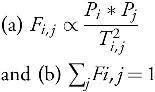
We then simulate a metapopulation SEIR (Susceptible-Exposed-Infectious-Recovered) model among the patches, with F_i,j representing the fraction of individuals from patch i spending their day in patch j on any given day. This approach is mainly used to mimic commuter-like mobility between the patches. More details on the method can be found in the literature.⁶⁰

Such a metapopulation model can be used for several purposes, such as disease forecasting and planning. In this example study, provided to illustrate the use of our mobility estimation methods, we will estimate early risk. To do so, we initialize the infections in the metapopulation model appropriately (n₀ initial cases in a seed patch i₀) and run the model forward with different levels of transmissibility β and time horizon T. At the end of T, after the epidemic has run its course, the cumulative risk is estimated for each patch as:

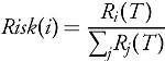
Where R_i(T) is the number of recovered individuals in patch i at time T. When coupled with a forecast, the projected risk is obtained by taking the proportion of incremental cases, instead of cumulative recovered cases.

We created 5 separate configuration stages for the most pressing North Kivu health zones: Mabalako, Beni, Butembo, Katwa, Kalnguta, and Oicha. Each configuration used uniform alpha and gamma parameters—in this case, 0.133 and 0.1, respectively—corresponding to an incubation period of 7.5 days and infectious period of 10 days.⁶¹ Meanwhile, variations were made to the beta parameters, the rate at which susceptible-infected contact results in new infections. These adjustments were made to approximate major inflection points of the different health zones, time points that likely coincided with newly introduced interventions or super-spreading events. We assume the true number of cases generally exceeds those observed; thus, the simulated case counts are generally higher than the observed ground truth being fitted.

Using case counts from January 23, 2019, the outbreak was calibrated both at the national and health zone levels (Figure 6). The mobility-linked health zones are independently calibrated at different inflection points to account for variations in the force of infection within the health zones themselves. In adjusting the beta parameter at each of the 5 stages, we found several interesting trends. First, we noticed a sharp increase in the rate of new infections in Beni from stage 1 (days 20 to 70) to stage 2 (days 70 to 110). To account for this, we increased the beta value by 92%. The ground data then experienced 3 approximate inflection points in stages 3 (days 110 to 140), 4, and 5. We accordingly decreased the beta value by around 50%, 33%, and 75%. This decrease illustrates a significant effect on the spread of Ebola in Beni.

Figure 6.

Cumulative case counts as reported through WHO situation reports are shown with a solid line; calibrated simulation curves shown with dashed lines approximate the course of the epidemic within each health district. Simulations are run 30 days past the last observation on January 24 (marked with grey vertical line at day 179) to produce 30-day risk estimates. Color images are available online.

Results

The resulting files from this methodological example as well as the travel matrix for DRC are included in the online supplemental materials (https://www.liebertpub.com/doi/suppl/10.1089/hs.2019.0101). Also included are the output from most steps in the attached methods guide.

Figure 7 compares the travel times derived from Euclidean distance calculations and a uniform speed to those derived from our network dataset. Although the 2 matrices share a mean travel time for all dyads, and a Pearson correlation of approximately 0.9, there are important disparities with individual pairings. For example, we notice that Beni, one of the epicenters of the 2019 outbreak, is much better connected to areas such as Mambasa, Musienene, and Oicha than would be expected from distance metrics alone. Conversely, it is far more distant from Tchomia and Mabalako than one would assume.

Figure 7.

A comparison between the origin-destination cost matrices, one derived using Euclidean distances with a uniform speed, the other using bimodal travel network built using the methodology presented in this article. Red values indicate that network travel time < Euclidean travel time, while black values indicate network travel time > Euclidean travel time. As we can see, most health zones are harder to reach than one would expect using Euclidean distance metrics alone. However, certain urban areas are highly connected, and travel times between them are even shorter than a distance model would predict. Color images are available online.

Figure 8 shows the predicted influence of Beni on neighboring zones of Nord Kivu as a function of disease mobility. In this case, we expect Katwa, a major city in the south, to be the most likely destination for new Ebola cases derived from the Beni outbreak. For the sake of comparison, Figure 9 shows the distance from Beni as a function of polygonal contiguity and Euclidean distance. Although the latter 2 are common metrics, they bear little resemblance to the interactions predicted by our mobility model.

Figure 8.

The influence that movement from Beni has on neighboring districts according to our completed mobility model. If Ebola does spread from Beni, we expect Katwa is the district most likely to suffer new cases. Color images are available online.

Figure 9.

The distance from Beni as a function of polygonal contiguity (left), and Euclidean distance (right). Neither is an accurate representation of mobility when modeling the spread of disease or detecting outbreaks. Note that Katwa and Butembo are not considered at great risk in these models. Color images are available online.

To provide an idea of what areas are at highest risk for future cases, we use the simulated case counts projected forward 30 days from January 23 and look at the relative proportions of cases generated in the health zones. The top 10 relative proportions of future cases are presented in Table 1, which, for the sake of comparison, also shows distance from Beni.

Table 1.

Relative Proportions of Cases Generated in the Health Zones

Health District	Future Case Proportion (%)	Polygonal Distance	Euclidean Distance (km)
Katwa	31.20	3	46.8
Butembo	7.70	3	47.6
Musienene	3.30	3	97.0
Kyondo	3.20	2	54.9
Lubero	3.10	4	84.4
Vuhovi	2.80	2	36.4
Mutwanga	2.70	2	34.9
Masereka	2.70	3	68.6
Kayna	2.20	2	120.1
Oicha	2.10	2	29.6

Discussion

These methods provide a novel means to quickly estimate mobility patterns in information-poor areas to support outbreak investigations. This allows us to put constraints on how people move about and transport diseases and can improve both outbreak detection and predictive modeling.

In our experience, one could follow the above procedures and supplemental guide and generate a transportation network in less than a day, with a mobility model deployed in less than a week. The results of such efforts could be used to improve predictive modeling or outbreak detection methods. Ignoring gravitational attractiveness of population centers produces unrealistic patterns of disease dissemination, as Figure 8 demonstrates. Furthermore, efforts that ignore network travel time miss the subtle variations in travel time that may drive the entire course of an epidemic. Consider again Figure 6: Despite the near identical mean travel time and 0.9 correlation coefficient, travel times from our outbreak's epicenter Beni to neighboring health zones varied by more than 50%. Those attempting to model the spread from that epicenter would be confounded using Euclidean distance alone, even if they accounted for gravitation attractiveness.

Our methodology is most suitable to real-time epidemic modeling efforts when rapid turnaround is required. This is particularly true in developing nations where curated travel network data are scarce. It is not an adequate replacement for a professionally curated travel network, and even less a replacement for calibrated mobility data informed by polling or cellular traffic. If such data are available for the study area and can be sourced in a timely manner, it is highly preferable to make use of them. If, however, no such data exist, we feel the method outlined above is an improvement over methods that are spatially agnostic.

Limitations

Estimating speed for rural roads in the developing world is particularly difficult. In truth, the speed is probably highly variable depending on the weather and method of transportation. Even on a major highway, a moped might travel half the speed of an automobile. On a rural route, we may need to include bicycles and animal carts. Similarly, we have no way of estimating the speed variability in river traffic or the effect of the river's current. This is not a critical flaw, however, as we are not concerned with explicit travel times, but rather the ratios of travel costs from each origin to each competing destination. So long as error introduced by inaccurate speed estimates is random across the network and each estimate is similarly affected, this should not be a substantial confounder. Another issue is the use of unpaved rural routes, which often wash out during periods of high rain. We have no means by which to account for network reliability without modeling flooding. That said, we are primarily focused on mobility between urban areas, and these areas experience the highest degree of road network centrality. Accordingly, it is difficult to isolate them completely.

Beyond that, the DCW data we used are quite out-of-date; new highways constructed between growing urban areas and newly constructed bridges are not accounted for. The method also assumes uniform rates of water-body crossings, but the schedule of ferries may confound travel time metrics. We are also unable to account for the effects of sociopolitical boundaries, including tribal affiliation, ethnicity, religion, and political affiliation. Such boundaries may be just as impassable as any river or mountain, and territorial disputes between government and rebel forces in DRC are currently confounding the Ebola response.^62-64 Also, nothing in methodology currently accounts for the fluctuations that an emerging infectious disease can introduce to human mobility. We feel this is a knowledge gap and worthy of further study. Many other methods of mobility estimation, including those based on historical cell tower records, also suffer the same challenges in making real-time inferences.

Finally, we note that uncertainty is difficult to quantify in such a study. The purpose of this method is to approximate mobility in an area with excessive data sparsity. As such, there are no competing models for comparison. There is uncertainty in both the shape and speed of the transportation network, but no obvious way to account for these in the absence of higher fidelity data. One could use competing transportation networks to increase confidence in our resulting origin-destination cost matrix, but again, such data are unavailable. Sensitivity could be modeled by introducing random variations in traversal speeds for each edge in the network and then repeating the analysis to determine how disease spread is affected. But rapid deployment is an integral feature of this methodology, and as such we did not delve further into sensitivity analysis.

Conclusion

This methodology allows one to rapidly create a transportation network and mobility model for use in epidemic response. It can be used to augment outbreak detection or forecast the spread of a disease, despite an absence of preexisting mobility data. We have demonstrated a potential use for these data in forecasting Ebola spread from Beni in the DRC. The method is not intended to replace curated mobility or transportation network data. However, in the event of an ongoing epidemic, when time is limited and data are scarce, it can improve on more traditional distance or polygonal contiguity-based analyses.

References

- 1. Gardner LI Jr, Brundage JF, Burke DS, McNeil JG, Visintine R, Miller RN. Spatial diffusion of the human immunodeficiency virus infection epidemic in the United States, 1985-87. Ann Assoc Am Geogr 1989;79(1):25-43 [Google Scholar]
- 2. Golub A, Gorr WL, Gould PR. Spatial diffusion of the HIV/AIDS epidemic: modeling implications and case study of AIDS incidence in Ohio. Geogr Anal 1993;25(2):85-100 [Google Scholar]
- 3. Wallace R, Wallace D. Socioeconomic determinants of health: community marginalisation and the diffusion of disease and disorder in the United States. BMJ 1997;314(7090):1341. [DOI] [PMC free article] [PubMed] [Google Scholar]
- 4. Pourrut X, Kumulungui B, Wittmann T, et al. The natural history of Ebola virus in Africa. Microbes Infect 2005;7(7-8):1005-1014 [DOI] [PubMed] [Google Scholar]
- 5. Breman JG, Piot P, Johnson KM, et al. The epidemiology of Ebola hemorrhagic fever in Zaire, 1976. Ebola virus Haemorrh fever 1978;103-124. http://www.enivd.de/EBOLA/ebola-24.htm Accessed January29, 2020
- 6. Baize S, Pannetier D, Oestereich L, et al. Emergence of Zaire Ebola virus disease in Guinea—preliminary report. N Engl J Med 2014;371(15):1418-1425 [DOI] [PubMed] [Google Scholar]
- 7. Bright EA, Rose AN, Urban ML. LandScan 2013 Global Population Database. East View Inf Serv ORN Lab. 2013
- 8. Wesolowski A, Buckee CO, Bengtsson L, Wetter E, Lu X, Tatem AJ. Commentary: containing the Ebola outbreak—the potential and challenge of mobile network data. PLoS Curr 2014;6. [DOI] [PMC free article] [PubMed] [Google Scholar]
- 9. Bell BP, Damon IK, Jernigan DB, et al. Overview, control strategies, and lessons learned in the CDC response to the 2014-2016 Ebola epidemic. MMWR Suppl 2016;65(3):4-11 [DOI] [PubMed] [Google Scholar]
- 10. Poletto C, Gomes MF, Pastore y Piontti A, et al. Assessing the impact of travel restrictions on international spread of the 2014 West African Ebola epidemic. Euro Surveill 2014;19(42):20936. [DOI] [PMC free article] [PubMed] [Google Scholar]
- 11. Gomes MF, Pastore y Piontti A, Rossi L, et al. Assessing the international spreading risk associated with the 2014 West African Ebola outbreak. PLoS Curr 2014;6. [DOI] [PMC free article] [PubMed] [Google Scholar]
- 12. Green A. Ebola outbreak in the DR Congo: lessons learned. Lancet 2018;391(10135):2096 [Google Scholar]
- 13. Munster VJ, Bausch DG, de Wit E, et al. Outbreaks in a rapidly changing Central Africa—lessons from Ebola. N Engl J Med 2018;379(13):1198-1201 [DOI] [PubMed] [Google Scholar]
- 14. Gostin LO. New Ebola outbreak in Africa is a major test for the WHO. JAMA 2018;320(2):125-126 [DOI] [PubMed] [Google Scholar]
- 15. Dudas G, Carvalho LM, Bedford T, et al. Virus genomes reveal factors that spread and sustained the Ebola epidemic. Nature 2017;544(7650):309-315 [DOI] [PMC free article] [PubMed] [Google Scholar]
- 16. Cliff AD, Haggett P, Ord JK, Versey GR. Spatial Diffusion: An Historical Geography of Epidemics in an Island Community. Cambridge: Cambridge University Press;1981 [Google Scholar]
- 17. Dorratoltaj N, Marathe A, Lewis BL, Swarup S, Eubank SG, Abbas KM. Epidemiological and economic impact of pandemic influenza in Chicago: priorities for vaccine interventions. PLoS Comput Biol 2017;13(6):e1005521. [DOI] [PMC free article] [PubMed] [Google Scholar]
- 18. Cenciarelli O, Pietropaoli S, Malizia A, et al. Ebola virus disease 2013-2014 outbreak in West Africa: an analysis of the epidemic spread and response. Int J Microbiol 2015;2015:769121. [DOI] [PMC free article] [PubMed] [Google Scholar]
- 19. Fisman D, Khoo E, Tuite A. Early epidemic dynamics of the West African 2014 Ebola outbreak: estimates derived with a simple two-parameter model. PLoS Curr 2014;6. [DOI] [PMC free article] [PubMed] [Google Scholar]
- 20. Althaus CL. Estimating the reproduction number of Ebola virus (EBOV) during the 2014 outbreak in West Africa. PLoS Curr 2014;6. [DOI] [PMC free article] [PubMed] [Google Scholar]
- 21. Pandey A, Atkins KE, Medlock J, et al. Strategies for containing Ebola in west Africa. Science 2014;346(6212):991-995 [DOI] [PMC free article] [PubMed] [Google Scholar]
- 22. Rivers CM, Lofgren ET, Marathe M, Eubank S, Lewis BL. Modeling the impact of interventions on an epidemic of Ebola in Sierra Leone and Liberia. PLoS Curr 2014;6. [DOI] [PMC free article] [PubMed] [Google Scholar]
- 23. Webb G, Browne C, Huo X, Seydi O, Seydi M, Magal P. A model of the 2014 Ebola epidemic in West Africa with contact tracing. PLoS Curr 2015;7. [DOI] [PMC free article] [PubMed] [Google Scholar]
- 24. Lewnard JA, Mbah MLN, Alfaro-Murillo JA, et al. Dynamics and control of Ebola virus transmission in Montserrado, Liberia: a mathematical modelling analysis. Lancet Infect Dis 2014;14(12):1189-1195 [DOI] [PMC free article] [PubMed] [Google Scholar]
- 25. Meltzer MI, Atkins CY, Santibanez S, et al. Estimating the future number of cases in the Ebola epidemic—Liberia and Sierra Leone, 2014-2015. MMWR Suppl 2014;63(3):1-14 [PubMed] [Google Scholar]
- 26. Halloran ME, Bharti N, Leora R, et al. Ebola: mobility data Ebola: public-private partnerships Ebola: Social research overlooked. Science 2014;346(6208):9-10 [Google Scholar]
- 27. Siettos C, Anastassopoulou C, Russo L, Grigoras C, Mylonakis E. Modeling the 2014 Ebola virus epidemic—agent-based simulations, temporal analysis and future predictions for Liberia and Sierra Leone. PLoS Curr 2015;7. [DOI] [PMC free article] [PubMed] [Google Scholar]
- 28. Merler S, Ajelli M, Fumanelli L, et al. Spatiotemporal spread of the 2014 outbreak of Ebola virus disease in Liberia and the effectiveness of non-pharmaceutical interventions: a computational modelling analysis. Lancet Infect Dis 2015;15(2):204-211 [DOI] [PMC free article] [PubMed] [Google Scholar]
- 29. Kramer AM, Pulliam JT, Alexander LW, Park AW, Rohani P, Drake JM. Spatial spread of the West Africa Ebola epidemic. R Soc Open Sci 2016;3(8):160294. [DOI] [PMC free article] [PubMed] [Google Scholar]
- 30. Yang W, Zhang W, Kargbo D, et al. Transmission network of the 2014-2015 Ebola epidemic in Sierra Leone. J R Soc Interface 2015;12(112):20150536. [DOI] [PMC free article] [PubMed] [Google Scholar]
- 31. Simini F, González MC, Maritan A, Barabási AL. A universal model for mobility and migration patterns. Nature 2012;484(7392):96-100 [DOI] [PubMed] [Google Scholar]
- 32. Crépey P, Barthélemy M. Detecting robust patterns in the spread of epidemics: a case study of influenza in the United States and France. Am J Epidemiol 2007;166(11):1244-1251 [DOI] [PubMed] [Google Scholar]
- 33. Viboud C, Bjørnstad ON, Smith DL, Simonsen L, Miller MA, Grenfell BT. Synchrony, waves, and spatial hierarchies in the spread of influenza. Science 2006;312(5772):447-451 [DOI] [PubMed] [Google Scholar]
- 34. Sattenspiel L, Dietz K. A structured epidemic model incorporating geographic mobility among regions. Math Biosci 1995;128:71-91 [DOI] [PubMed] [Google Scholar]
- 35. Xia Y, Bjørnstad ON, Grenfell BT. Measles metapopulation dynamics: a gravity model for epidemiological coupling and dynamics. Am Nat 2004;164(2):267-281 [DOI] [PubMed] [Google Scholar]
- 36. Black WR. Flow network autocorrelation in transport network and flow systems. Geogr Anal 1992;24(3):207-222 [Google Scholar]
- 37. Mclafferty S. Disease cluster detection methods: recent developments and public health implications. Ann GIS 2015;21(2):127-133 [Google Scholar]
- 38. Alexander KA, Lewis BL, Marathe M, Eubank S, Blackburn JK. Modeling of wildlife-associated zoonoses: applications and caveats. Vector Borne Zoonotic Dis 2012;12(12):1005-1018 [DOI] [PMC free article] [PubMed] [Google Scholar]
- 39. Newman MEJ. Spread of epidemic disease on networks. Phys Rev E 2002;66(1):1-11 [DOI] [PubMed] [Google Scholar]
- 40. Meyers LA, Pourbohloul B, Newman MEJ, Skowronski DM, Brunham RC. Network theory and SARS: predicting outbreak diversity. J Theor Biol 2005;232(1):71-81 [DOI] [PMC free article] [PubMed] [Google Scholar]
- 41. Levin SA, Grenfell B, Hastings A, Perelson AS. Mathematical and computational challenges in population biology and ecosystems science. Science 1997;275(5298):334-343 [DOI] [PubMed] [Google Scholar]
- 42. Shirley MDF, Rushton SP. The impacts of network topology on disease spread. Ecol Complex 2005;2(3):287-299 [Google Scholar]
- 43. van den Driessche P. Spatial structure: patch models. In: Brauer F, Wu J, van den Driessche, eds. Mathematical Epidemiology. Berlin: Springer-Verlag; 2008:179-189 [Google Scholar]
- 44. Riley S. Large-scale models of infectious disease. Science 2007;316(June):1298-1301 [DOI] [PubMed] [Google Scholar]
- 45. Doungmo Goufo EF, Oukouomi Noutchie SC, Mugisha S. A fractional SEIR epidemic model for spatial and temporal spread of measles in metapopulations. Abstr Appl Anal 2014;2014 [Google Scholar]
- 46. Lunelli A, Pugliese A, Rizzo C. Epidemic patch models applied to pandemic influenza: contact matrix, stochasticity, robustness of predictions. Math Biosci 2009;220(1):24-33 [DOI] [PubMed] [Google Scholar]
- 47. Njagarah JBH, Nyabadza F. A metapopulation model for cholera transmission dynamics between communities linked by migration. Appl Math Comput 2014;241:317-331 [Google Scholar]
- 48. Hickson RI, Mercer GN, Lokuge KM. A metapopulation model of tuberculosis transmission with a case study from high to low burden areas. PLoS One 2012;7(4) [DOI] [PMC free article] [PubMed] [Google Scholar]
- 49. Riley S. Models of infectious disease. Science 2007;316(5829):1298-1301 [DOI] [PubMed] [Google Scholar]
- 50. Truscott J, Ferguson NM. Evaluating the adequacy of gravity models as a description of human mobility for epidemic modelling. PLoS Comput Biol 2012;8(10) [DOI] [PMC free article] [PubMed] [Google Scholar]
- 51. Ren Y, Ercsey-Ravasz M, Wang P, González MC, Toroczkai Z. Predicting commuter flows in spatial networks using a radiation model based on temporal ranges. Nat Commun 2014;5:5347. [DOI] [PubMed] [Google Scholar]
- 52. Delmelle EM, Marsh DM, Dony C, Delamater PL. Travel impedance agreement among online road network data providers. Int J Geogr Inf Sci 2019;33(6):1251-1269 [Google Scholar]
- 53. Danko DM. The digital chart of the world project. Photogramm Eng Remote Sens 1992;58:1125-1128 [Google Scholar]
- 54. Foster V, Benitez DA. The Democratic Republic of Congo's Infrastructure: A Continental Perspective. Washington, DC: World Bank; 2010. http://documents.worldbank.org/curated/en/901171468191948305/pdf/623860WP0P12420ort0final0Image0Bank.pdf Accessed January29, 2020 [Google Scholar]
- 55. Wu Q, Merchant F, Castleman KR, eds. Microscope Image Processing. Burlington, MA: Elsevier; 2010 [Google Scholar]
- 56. HDX. Democratic Republic of Congo and neighboring countries health boundaries. 2018. https://data.humdata.org/dataset/democratic-republic-of-congo-health-boundaries Accessed January29, 2020
- 57. Linard C, Gilbert M, Snow RW, Noor AM, Tatem AJ. Population distribution, settlement patterns and accessibility across Africa in 2010. PLoS One 2012;7(2):e31743. [DOI] [PMC free article] [PubMed] [Google Scholar]
- 58. Marathe MV, Vullikanti AKS. Computational epidemiology. In: Proceedings of the 20th ACM SIGKDD International Conference on Knowledge Discovery and Data Mining. New York; 2014 [Google Scholar]
- 59. Daley DJ, Gani J. Epidemic Modelling: An Introduction. Cambridge: Cambridge University Press; 2001 [Google Scholar]
- 60. Venkatramanan S, Chen J, Gupta S, et al. Spatio-temporal optimization of seasonal vaccination using a metapopulation model of influenza. In: Healthcare Informatics (ICHI), 2017. Ieee International Conference;2017:134-143 [Google Scholar]
- 61. Camacho A, Kucharski AJ, Funk S, Breman J, Piot P, Edmunds WJ. Potential for large outbreaks of Ebola virus disease. Epidemics 2014;9(2014):70-78 [DOI] [PMC free article] [PubMed] [Google Scholar]
- 62. Moran B. Fighting Ebola in conflict in the DR Congo. Lancet 2018;392(10155):1295-1296 [DOI] [PubMed] [Google Scholar]
- 63. Arie S. Rebel attacks and political scaremongering raise risk of Ebola spreading in the Congo. BMJ 2018;362:k4117. [DOI] [PubMed] [Google Scholar]
- 64. Cousins S. Violence and community mistrust hamper Ebola response. Lancet Infect Dis 2018;18(12):1314-1315 [DOI] [PubMed] [Google Scholar]
Associated Data
This section collects any data citations, data availability statements, or supplementary materials included in this article.