Multi-pathway multi-echo acquisition and neural contrast translation to generate a variety of quantitative and qualitative image contrasts

Abstract

Purpose:

Clinical exams typically involve acquiring many different image contrasts, to help discriminate healthy from diseased states. Ideally, 3D quantitative maps of all of the main MR parameters would be obtained for improved tissue characterization. Using data from a 7-min whole-brain multi-pathway multi-echo (MPME) scan, we aimed to synthesize several 3D quantitative maps (T₁ and T₂) and qualitative contrasts (MPRAGE, FLAIR, T₁-weighted, T₂-weighted and proton density (PD)-weighted). The ability of MPME acquisitions to capture large amounts of information in a relatively short amount of time suggests it may help reduce the duration of neuro MR exams.

Methods:

Eight healthy volunteers were imaged at 3.0T using a 3D isotropic (1.2 mm) MPME sequence. Spin-echo, MPRAGE and FLAIR scans were performed for training and validation. MPME signals were interpreted through neural networks for predictions of different quantitative and qualitative contrasts. Predictions were compared to reference values at voxel and region-of-interest levels.

Results:

Mean absolute errors (MAEs) for T₁ and T₂ maps were 216 ms and 11 ms, respectively. In ROIs containing white matter (WM) and thalamus tissues, the mean T₁/T₂ predicted values were 899/62 ms and 1139/58 ms, consistent with reference values of 850/66 ms and 1126/58 ms, respectively. For qualitative contrasts, signals were normalized to those of WM, and MAEs for MPRAGE, FLAIR, T₁-weighted, T₂-weighted and PD-weighted contrasts were 0.14, 0.15, 0.13, 0.16 and 0.05, respectively.

Conclusions:

Using an MPME sequence and neural-network contrast translation, whole-brain results were obtained with a variety of quantitative and qualitative contrast in about 6.8 minutes.

Introduction

MRI exams typically involve a number of different pulse sequences that generate a number of different image contrasts. However, only a handful of basic MR parameters are at the source of these various contrasts. If these parameters could be rapidly and quantitatively evaluated, then most of the information MRI has to offer would be quickly harvested, opening the door for MRI exams of considerably reduced duration. Furthermore, quantitative parameter maps lend themselves to the use of threshold values that have physical meaning and rationale, and as such they may prove better-suited for discriminating healthy and diseased states compared to more traditional qualitative MRI contrasts. Synthetic imaging involves using quantitative knowledge about tissues, toward emulating the qualitative grayscale contrasts that would have been obtained if scans had been performed using given pulse sequences.

Motivated by the considerable promise of quantitative MRI, several different methods have been introduced over the years toward this goal. These may differ in a number of ways, most notably on the particular set of parameters they can map, whether these parameters are captured jointly or in a serial manner, and on the overall scan efficiency of the approach. For example, over the years, methods have been proposed that evaluate the longitudinal relaxation (T₁) (1-4), the transverse relaxation (T₂ and T₂*) (5-8), susceptibility effects (9-11), the apparent diffusion coefficient (ADC) (12-14) or the B₁⁺ field (15-17). As such, one could readily string together several of these mapping methods and, in the process, map multiple parameters. However, scan time could readily grow beyond reasonable bounds when compounding several methods in such manner. Other, sometimes more elaborate methods may be geared instead toward jointly estimating several parameters (18-21).

The methodology developed here can jointly map a few of the main MR parameters while also synthesizing some of the main image contrasts typically employed in clinical neuroradiology. The proposed approach involves a single 3D scan, with all required contrasts sampled every TR, which in principle should provide robustness to geometrical distortion and/or motion. The rich information content harvested by the proposed multi-pathway multi-echo (MPME) pulse sequence is translated into better-known and arguably more useful image contrasts, and this ‘contrast translation’ is performed using machine learning methods. More generally, the purpose of this study was to achieve a variety of quantitative and qualitative contrast types, over a relatively short period of time, with whole-brain coverage and spatial resolution consistent with current clinical neuroimaging protocols.

Methods

Magnetization pathways and MPME acquisition

Magnetization pathways are typically numbered such that the 0^th pathway is found nearest to k-space center flanked by the +1^st and −1^st, in opposite k-space directions, while higher-numbered pathways are found increasingly far from the 0^th pathway and tend to offer increasingly small signals. Acquisition of multiple signal pathways was introduced about 30 years ago (22-24), and a number of dedicated imaging sequences have been developed since, most notably DESS (25) (2 pathways: 0^th and –1^st) and TESS sequences (20) (3 pathways: +1^st, 0^th, and –1^st). Going a step further, we developed a multi-pathway sequence that acquires multiple pathway signals at a few different echo times every TR. In prior work (21), this multi-pathway multi-echo (MPME) sequence was applied to the problem of quantitative MRI, and 3D parameter maps were analytically calculated from the MPME signals for T₁, T₂, T₂*, M₀, B₀ and B₁⁺. Because T₁ and B₁⁺ information are entangled in most signals acquired by MRI, the accurate mapping of T₁ often requires some knowledge of B₁⁺ to be available as well; as shown in Fig. 1, a strength of MPME imaging is that different pathway signals tend to capture variations in T₁ and B₁⁺ differently thus providing information about both (simulation performed with TR = 20 ms; T₂ = 100 ms; T₂* = T₂; −2^nd, −1^st, 0^th, +1^st and +2^nd pathways; flip angles ranging from 1 to 45°, T₁ values from 100 to 1200 ms). Compared to the prior work in Ref. (21), the present MPME acquisition gathers four pathways (instead of three), at two different echo times (instead of three), and signals are interpreted through neural networks (instead of analytically), to generate a combination of quantitative and qualitative contrasts relevant to neuroradiology (instead of only quantitative maps).

Fig 1:

The present simulation shows how signals from different pathways can behave very differently as the flip angle and/or T₁ are varied. Signals from −2^nd (a), −1^st (b), 0^th (c) +1^st (d), and +2^nd (e) pathway were scaled differently for optimized illustration in the same color scale. The notation F_i⁺ refers to the steady-state signal from the i^th pathway right after an RF pulse. For T₁ values typically associated with biological tissues at 3T (e.g. T₁ ~ 1000 ms), the signal strength of the +2^nd pathway was noticeably weaker than those of other pathways, and for this reason the +2^nd pathway was not sampled here.

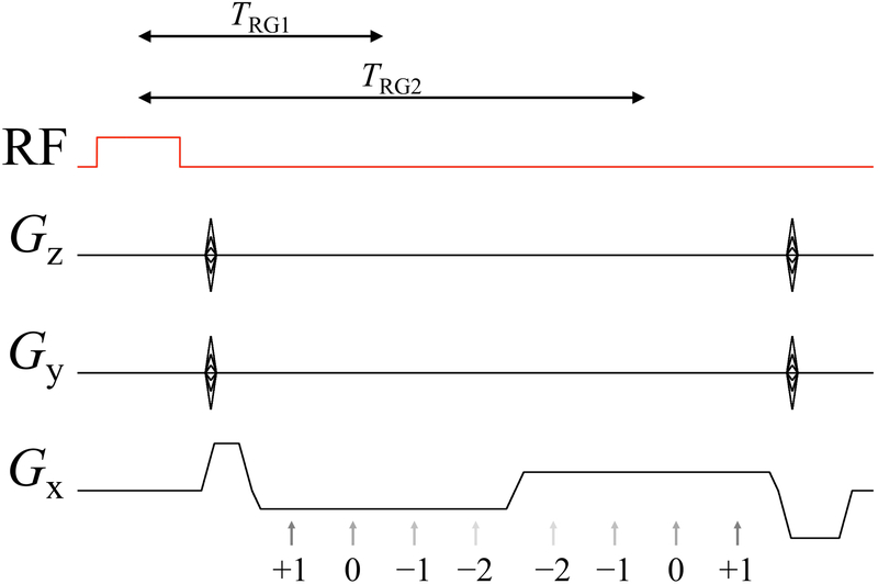
As depicted in Fig. 2, all four pathways were sampled in two macro-readout windows, leading to 8 separate 3D k-space matrices for image reconstruction, i.e., pathway signals were extracted from the macro-readout window and reconstructed separately. The readout direction was placed along B₀, and a PROPELLER-like scheme (26, 27) was implemented in the k_y-k_z plane to repeatedly sample the central k-space region for increased motion robustness. Acceleration was achieved with a non-uniform subsampling scheme (28) and associated parallel imaging reconstruction. Compared to rectangular Cartesian sampling, the combined effect of PROPELLER-like over-sampling and non-uniform under-sampling gave a net acceleration factor of about 1.55. The resulting sampling pattern in the k_y-k_z plane is depicted in Fig. 3. Spatial resolution and acceleration factor were kept constant for all volunteers, and as a consequence small variations in head size and FOV among volunteers led to corresponding variations in matrix size and scan time (see Table 1).

Fig 2:

A 3D multi-pathway multi-echo (MPME) sequence of our own design was used to acquire four signal pathways at 2 different echo times. The numerals indicate the pathway number, from −2^nd to +1^st, and the gray arrows indicate the timing of each signal formation. T_RG1 and T_RG2 define the length of the time interval from the center of the RF pulse to the center of the corresponding readout group, i.e., T_RG is to readout groups what TE would be to individual echoes.

Fig 3:

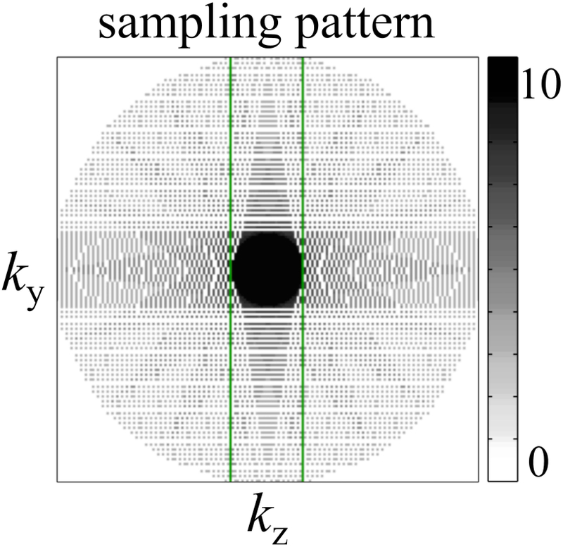
In a manner that bears resemblance to the PROPELLER acquisition scheme, the k_y-k_z plane was covered using a series of rotated blades, e.g., see green rectangle. The acquisition of each blade was accelerated using a non-linear subsampling scheme. Because all blades combine at the center the overall effect was to oversample the central region, thus providing resilience in the presence of motion. By oversampling the center while subsampling the edges, the net result was an acceleration factor of roughly 1.55-fold compared to a full Cartesian sampling. The grayscale bar shows the overall sampling density of the k-space acquisition.

Table 1:

MR imaging sequence parameters. Reference T₁- and T₂-weighted images are marked with bold font.

MPME scans	Number of pathways	TRG (ms)	TR (ms)	Flip angle (°)	Matrix size	Pixel bandwidth (Hz/pixel)	Voxel size (mm3)	Accel. factor	Acquisition time
volunteer #1-7	4	6.3, 13.1	20	15	160×176×176	638	1.2×1.2×1.2	1.55	6:41
volunteer #8	4	6.3, 13.1	20	15	160×192×192	638	1.2×1.2×1.2	1.54	7:58
Reference scans	TI (ms)	TE (ms)	TR (ms)	Flip angle (°)	Number of slices	Pixel bandwidth (Hz/pixel)	Voxel size (mm3)	Accel. factor	Acquisition time
MPRAGE	900	3.76	1750	9	192	260	1.2×1.2×1	2	3:42
FLAIR	2026.6	88	6000	130	29	260	1.2×1.2×3	2	1:38
SE	N/A	25, 50, 90, 120	1000	90/180	5	260	1.2×1.2×2	1	10:48
IR-SE	50, 300, 800, 2400	10	2500	180/90/ 180	1	260	1.2×1.2×2	2.67	12:20

Abbreviation: T_RG, time to readout group; Accel, acceleration; SE, spin echo; IR-SE, inversion-recovery spin echo; N/A, not applicable.

Subject recruitment and MR scans

Eight healthy volunteers (1/7 female/males, 32.0±8.8 years old) were scanned, following informed consent using an IRB-approved protocol. All imaging scans were performed on a 3.0T Trio system (Siemens Healthineers, Erlangen, Germany) using a product 12-channel head matrix. TR for the MPME scan was set near its minimum possible value, for the gradient strength and slew rate available on this particular scanner and the selected spatial resolution (1.2 mm isotropic).

Further scans, with product pulse sequences, were required for training and validation purposes. More specifically, the ‘magnetization prepared rapid gradient-echo’ (MPRAGE) (29), the ‘fluid-attenuated inversion recovery’ (FLAIR) (30), the spin-echo (SE) and the inversion-recovery SE (IR-SE) product sequences were employed. 2D single-echo SE scans were performed sequentially using four different TE settings, allowing T₂ to be calculated. Similarly, 2D IR-SE scans were performed with four different inversion time (TI) settings, allowing T₁ to be calculated. The 2D SE and IR-SE scans were performed for only one axial slice per volunteer, selected to contain key brain structures such as the caudate nucleus, putamen and/or thalamus. The MPRAGE and FLAIR sequences were chosen because they are common components of clinical neuroimaging protocols. Scan parameters are listed in Table 1; SE scans performed with the setting TE = 90 ms were interpreted here as models of T₂-weighted contrast to be emulated through contrast translation, and similarly, IR-SE scans performed with TI = 800 ms were interpreted as models of T₁-weighted contrast to be emulated here.

Image reconstruction

Raw data were collected for all scans and were reconstructed off-line. Through zero-filling, the reconstructed matrix size and resolution were adjusted so that all scans for a given volunteer would have matching voxel locations. Software from the BART toolbox (31) and the NCIGT fast-imaging library (32) were employed for reconstruction. Processing was performed in Matlab (R2010a, 64-bit) on a 64-bit linux machine (Intel i7–4820K 3.7GHz, 64GB of memory). Using one of the 2D T₂-weighted SE images (TE = 90 ms) as a reference, the best-matching slice from the 3D MPME and MPRAGE scans were selected. As a result, a collection of 18 different images with different contrasts were available for this same 2D axial slice: 8 images from the MPME scan (4 pathways × 2 echo times), 4 from the SE scans performed with different TE settings, 4 from the IR-SE scans performed with different TI settings, 1 from MPRAGE and 1 from FLAIR.

Images acquired with different sequences may be distorted in different ways and volunteers may move during their exam; for these reasons, a registration step was included in the reconstruction process. Still using the TE = 90 ms 2D SE image as a reference, all other images were registered to it using the six degree-of-freedom registration algorithm FLIRT (FSL, Oxford, UK) (33). Worth noting, a fully-trained version of the proposed method would not require any such registration step, as all acquired data would come from the same MPME scan. The registration step is needed here only for training and validation purposes, so that reference and MPME data could be mixed and compared on a pixel-by-pixel basis.

Reference T₁ and T₂ maps were calculated from the SE and IR-SE images, respectively. A proton density (PD)-weighted image was also calculated by removing the T₂ weighting from the S₀ map as obtained through the T₁ fit. A mask that selected brain tissues and removed background signals was generated using the BET software (33) to mask out background voxels before performing machine learning. Again, a fully-trained version of the proposed method would not require such background-masking step, but it was needed here to limit training and validation to signal-containing voxels.

Generating contrasts, first step: B₀ maps were evaluated in a conventional manner

In a first step, B₀ maps were calculated using a linear regression of the phase information from the multi-TE MPME data. Weights were used to inhibit phase noise from pathway images with lower SNR. Alternately, one could include B₀ in the training step below and rely on machine learning for evaluation. In our experience, because MPME scans readily provide the needed multi-echo information, it was preferable to calculate B₀ separately and, in so doing, to keep the machine-learning step as lean and straightforward as possible. B₀ maps were obtained by unwrapping the phase information with PRELUDE (33) and then performing a weighted linear regression with respect to TE. Different pathways provided different measurements of B₀, which were combined in an SNR-optimum fashion as described in (34). Once phase information was converted into B₀ maps, there was no further need for the phase channel of the MPME images and all further processing steps were performed on magnitude data.

Generating contrasts, second step: T₁, T₂, T₁-, T₂-, PD-weighted, MPRAGE and FLAIR

A multilayer perceptron (MLP) or feedforward neural network (NN) was employed here to learn a mapping from MPME signals to the desired image contrasts and maps. An underlying assumption of the present work is that neighboring voxels can contain different tissue types and as such should be considered mostly independent. Convolutional neural networks (CNNs), the most popular type of neural architecture used in image processing, as used in computer vision and image synthesis, are working on pixel regions, and for this reason did not prove well-suited for voxel-by-voxel contrast translation. As for recurrent neural networks (RNNs), they are typically employed to treat time-dependent data, which is not necessarily the case here. The present application involved a relatively small number of inputs and presumably for this reason a relatively simple NN proved appropriate.

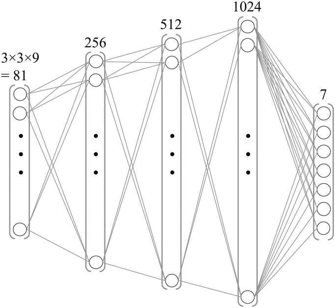
While voxel-by-voxel processing was desired, signal may readily bleed from one voxel to the next due to the shape of the imaging point-spread-function, motion and/or errors in registration. For this reason, a 3×3 window was extracted around each voxel. Nine different input contrast channels were available per voxel: the 8 MPME signals (4 pathways × 2 echo times) and the B₀ value as calculated above. Accordingly, the number of input values was the window size times the number of contrast channels, 3×3×9=81. These 81 input values were flattened into a vector to form the network input (see Fig. 4). In contrast, there were only 7 output channels: T₁, T₂, T₁-weighted (TI = 800 ms), T₂-weighted (TE = 90 ms), PD-weighted, MPRAGE-like and FLAIR-like contrasts for a given voxel, the one located in the middle of the 3×3 patch. The model architecture consisted of three hidden layers with rectified linear unit activation, and an output layer with linear activation. The number of neurons in the hidden layers increased with depth (256, 512 and 1024, respectively). The total number of trainable parameters of the network was 727,052. The mean absolute error was employed as the loss function, and the Adam update rule (with learning rate = 1e−5, beta₁ = 0.9, beta₂ = 0.999) was used to train the network using the backpropagation algorithm (35). The network was implemented using Keras v.2.2.0 (Tensorflow 1.5.0 backend) in Python 3.6 and trained on an Nvidia Titan Xp GPU (Nvidia Corporation, Santa Clara, CA, USA). The NN was trained to emulate the following quantitative and qualitative contrasts (Table 1): T₁, T₂, MPRAGE, FLAIR, IR-SE T₁-weighted (TI = 800 ms), SE T₂-weighted (TE = 90 ms), and PD-weighted contrasts. Image reconstruction was performed by sequentially feeding each 1×1×81 tensor to the network and obtaining a tensor of size 1×1×7 representing these seven output contrasts for the central voxel. Presumably due to the relatively small size of the network along with good information content at the input, regularization was not required here.

Fig. 4:

Schematic representation of the four-layer NN employed here. It accepted 81 entries in its input layer and generated 7 values in its output layer (T₁, T₂, MPRAGE, FLAIR, T₁-, T₂-, and PD-weighted).

Proper scaling was crucial as neural networks learn by minimizing prediction errors, which tend to scale with the size of the signal being predicted. For example, because T₁ tends to be an order of magnitude or so larger than T₂, unscaled training would tend to place greater emphasis on correctly predicting T₁ compared to T₂, while placing arbitrary importance to arbitrarily-scaled signals such as MPRAGE or FLAIR. For these reasons, all 88 channels involved in training (81 input and 7 output channels) were scaled to fit between 0 and 1. Scaling factors were identical for all volunteers, and the scaling was inverted after NN predictions to recover quantitative maps with proper physical scaling. More specifically, the input T₁, T₂, and B₀ values were scaled by 1/4000 ms, 1/200 ms and 1/180 Hz, respectively, while the scaling required for the arbitrarily-scaled T₁-, T₂-, and PD-weighted, MPRAGE, FLAIR and each one of the MPME pathway is of little interest here, except to say that the same scaling factor was used for both echoes of the MPME acquisition. After scaling, wherever/whenever needed, all channels were truncated to fit between 0 and 1.

As a direct consequence of the present voxel-by-voxel processing, a large number of separate ‘experiments’ were available for training and validation purposes. Excluding dark voxels located in air, each volunteer contributed on average about 12,300 signal-containing voxels. Data from seven out of eight subjects were used for training, which amounted to about 86,100 voxels, while data from the remaining subject was used for validation. More specifically, a leave-one-out approach was implemented: validation results for volunteer number n were obtained by training a network, NN_n, using data from all volunteers but volunteer number n. With n ranging from 1 to 8, a total of eight separately-trained but presumably similar NNs were obtained. This leave-one-out approach allowed a relatively large number of data points to be used for training and a relatively large number of data points to be generated for validation, while still ensuring that separate data were used for the two.

To test the effect of N, the number of recruited volunteers, reconstructions were performed while varying N from its actual (maximal) value of N=8 all the way down to N=2, whereby one volunteer would provide training data and the other volunteer would provide validation data. More specifically, for each volunteer number n ranging from 1 to 8, and with N ranging from 2 to 8, then (N−1) volunteers other than volunteer number n were randomly shuffled for training purposes. These results were used to help evaluate the effect of N, in the range from 2 to 8.

Validation

Once a given network had been trained, it could convert a 3D MPME dataset into 3D maps of T₁, T₂, MPRAGE, FLAIR, T₁-weighted, T₂-weighted, and PD-weighted contrasts. However, reference results derived from the 2D SE and 2D IR-SE scans were available only over a single 2D plane within this 3D volume. For this reason, validation could only be performed over the 2D plane where reference results and MPME-derived results were both available. As stated above, such 2D plane contributed on average about 12,300 signal-containing voxels per volunteer, which means that all eight volunteers combined into about 98,400 data points for validation purposes.

Predicted and reference values were compared, for each one of the seven quantitative and qualitative contrasts generated by the NNs. Using T₁ as an example, the error on T₁, (T_1,NN – T_1,ref), was plotted against the mean value, (T_1,NN + T_1,ref)/2. This is very similar to a Bland-Altman plot, except for the fact that the Bland Altman method requires independent measurements while repeated measurements at different location (voxels) were available here instead. Due to the relatively large number of data points per plot, about 98,400 of them, the density of points was displayed as a grayscale as opposed to plotting individual points. In addition to global (i.e., whole brain) analysis as described above, white matter and thalamus ROIs were manually contoured in both reference and prediction maps for T₁ and T₂, enabling an ROI-based (as opposed to pixel-based) validation step.

Results

Training

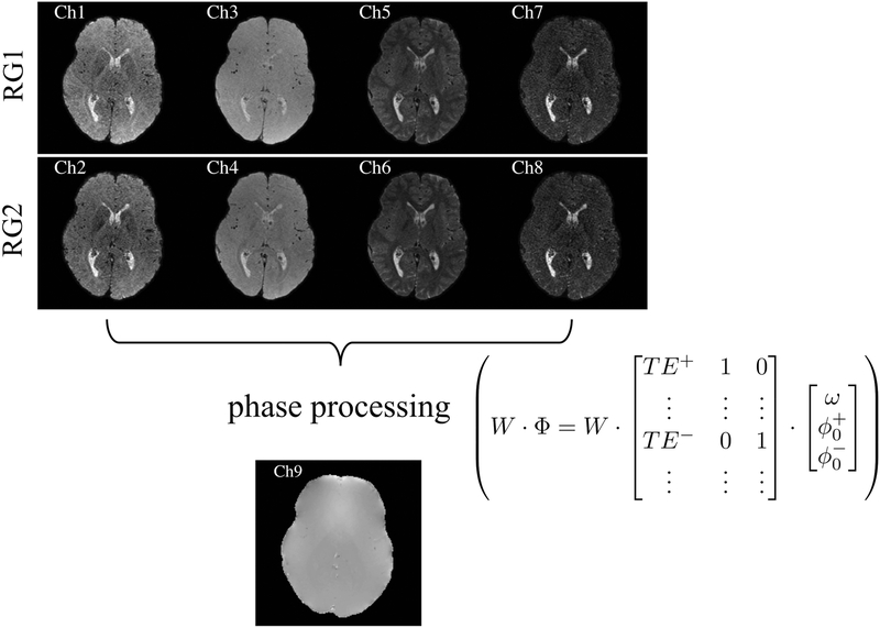
Figure 5 shows the type of MPME-related information that was provided as input to the NNs: four different pathways [−2, −1, 0, +1] at two different echo times, as well as a field map (B₀). Note how different the image contrast can be from one pathway to the next; these differences in contrast further confirm what was suggested by simulations in Fig. 1, i.e., that different pathways contribute very different information content. Training was performed for 40 epochs, which was empirically determined to prevent model overfitting. We have found the choice of training epochs to be a forgiving hyper-parameter as similar convergence behavior and visual results have been obtained with a range of settings, without overfitting; more specifically similar results were obtained with 20 or 40 epochs, and results for 40 epochs are reported here. The average training time for one single NN was 40±1 s, and it took another 102±1 s on average to perform contrast translation for the whole brain volume. In an ideal scenario, all of the trained networks would be identical, but of course in practice they would not be expected to be so. As usual with NNs, individual values at individual neurons could not readily be interpreted in meaningful ways, and the same can be said of their differences. But the rationale for training eight separate networks was that for each volunteer, different data were used for training and for validation purposes.

Fig. 5:

Inputs to the NN came from 9 different types of MR-related signals: 4 pathways acquired twice in 2 separate readout groups (RG), along with B₀ information. For each voxel location of the output, a 3×3 patch centered on that location was selected at the input, leading to 3×3×9=81 values in the input layer. The phase processing consisted of a weighted linear regression that equalized the phase noise in all pathway images, for optimum field map estimation, ω. The ‘+’ and ‘−’ signs refer to positive and negative pathways, respectively.

Validation

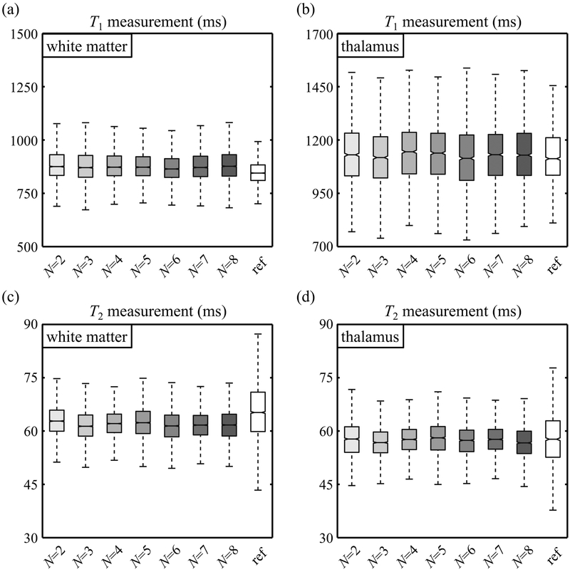
T₁ and T₂ predictions obtained while varying the number of volunteer datasets, N, are shown in Fig. 6 for white matter (Fig. 6a, c) and thalamus tissues (Fig. 6b, d). These results showed only subtle N-related effects. Images in Fig. 7 were meant to visually emphasize and help appreciate the 3D nature of the datasets generated by the proposed method. All of these contrasts were, by nature, essentially perfectly registered to each other as they all stemmed from the same 3D MPME dataset. In contrast, the validation process in Fig. 8 and 9 involved only one single 2D slice extracted from the 3D MPME-derived results, to spatially match the 2D reference data. It is worth noting that the acquisition of reference data occupied most of the acquisition time in the overall exam (see Table 1) even though such reference data were in most cases only available over a 2D slice.

Fig. 6:

The purpose of these results was to explore the effect of N, the number of volunteers, on predicted T₁ (a-b) and T₂ (c-d) values. The number of subjects was varied from its actual (maximal) value of 8 all the way down to 2, whereby data from only one volunteer would be used for training and one for validation purposes. Reference T₁ and T₂ values are tagged with ‘ref’ for comparison. Overall, there were no drastic observable effect/improvement as N is increased beyond two possibly because: 1) each volunteer contributes about 12,000 signal-containing voxels, 2) the NN is fairly simple and trained on a per-voxel basis, 3) the main limiting factor at this point might be the spatial alignment of MPME and training data, an effect that might hide more subtle N-related effects.

Fig. 7:

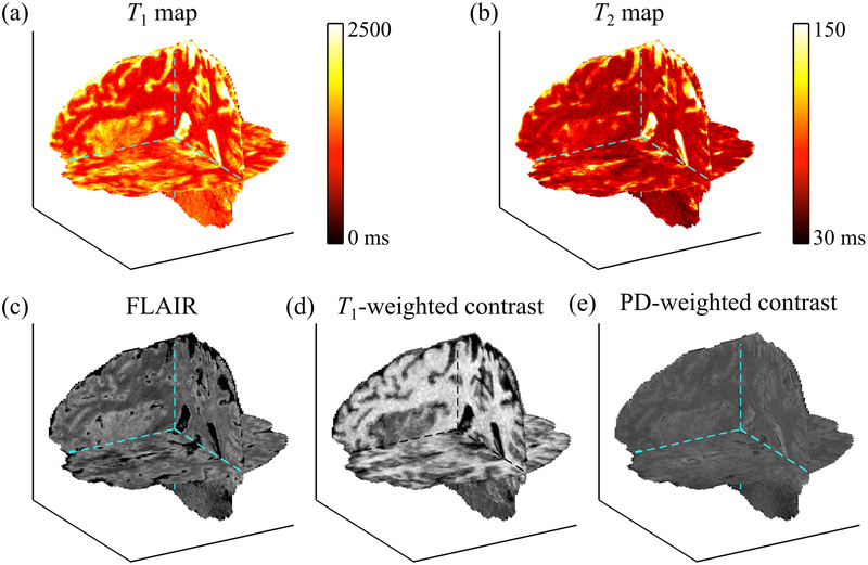
The proposed method achieved whole-brain 3D coverage with isotropic resolution, as visually emphasized here in (a) T₁ map, (b) T₂ map, (c) FLAIR, (d) T₁-weighted, and (e) PD-weighted contrasts. These contrasts would typically have to be acquired using separate pulse sequences, while they were all generated from one single MPME scan here through neural contrast translation.

Fig. 8:

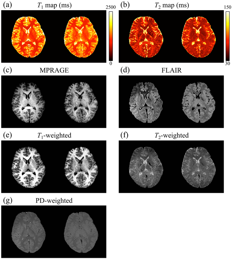
A side-by-side comparison of reference (left) and NN-predicted values (right) is shown for one representative subject (volunteer 3). Results were qualitatively similar for other subjects, and data from all subjects were included in the quantitative evaluation presented in Fig. 9 and in Supporting Information Figure S1. While reference results were available only over the 2D slice shown here, the predicted results were available over the whole brain as visually emphasized in Fig. 7.

Fig. 9:

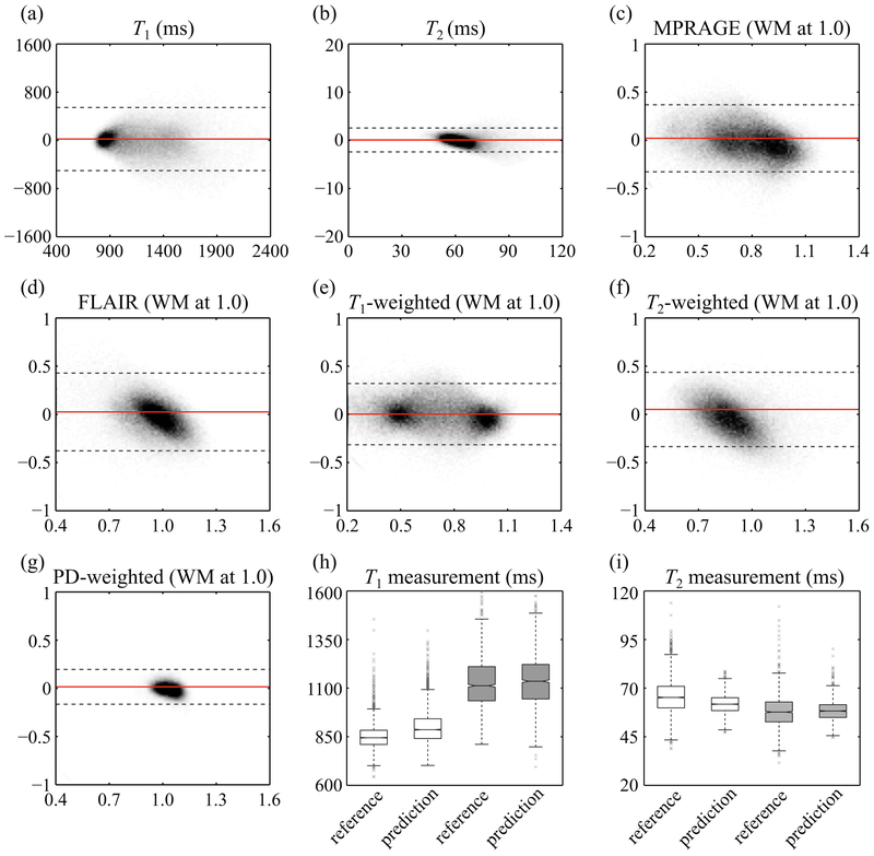
Reference and predicted results were compared, for each one of the predicted signal types (T₁, T₂, MPRAGE, FLAIR, T₁-, T₂-, and PD-weighted). Each plot, similar to a Bland-Altman analysis, combines results from all volunteers. Plots in (c-g) were normalized by defining ‘1.0’ as the signal level of white matter. Gray dashed lines represent the 95% limits of agreement, and solid red lines show the bias. Quantitative T₁ (h) and T₂ (i) values were further compared, for reference and predicted results, based on white matter (white boxes) and thalamus (gray boxes) ROIs. The plots in (h,i) combine data from all 8 subjects. Outliers are shown with gray ‘×’ markers.

Figure 8 shows side-by-side comparisons between reference and predicted results for one subject (volunteer #3), and a full comparison of all 8 volunteers is provided in the same format in Supporting Information Figure S1. Figure 9 includes data from all subjects and compares predicted and reference values for all 7 contrasts generated here: T₁, T₂, MPRAGE, FLAIR, T₁-weighted, T₂-weighted, and PD-weighted contrasts. In Fig. 9c-g, scaling was arbitrary, and signals were normalized so that a value of ‘1.0’ represented the signal strength of white matter for this particular contrast type. More specifically, the mean value of the white matter ROI was used to normalize both axes of the corresponding results, which is similar to a Bland-Altman plot. The mean absolute error for quantitative T₁ and T₂ maps were 216 and 11 ms, respectively. Those for MPRAGE, FLAIR, T₁-weighted, T₂-weighted, and PD-weighted contrasts were 0.14, 0.15. 0.13, 0.16 and 0.05, respectively. The 95% limits of agreement were 1061 and 51 ms for T₁ and T₂, and 0.69, 0.69, 0.63, 0.77, and 0.27 for MPRAGE, FLAIR, T₁-weighted, T₂-weighted, and PD-weighted contrasts, respectively.

Looking at ROIs for white matter and thalamus tissues, the predicted T₁ and T₂ values were found comparable to reference values (Fig. 9h-i). More specifically, predicted and reference values in white matter were (mean ± standard deviation): 899±87 and 850±63 ms for T₁, 62±5 and 66±9 ms for T₂, respectively. In the thalamus predicted and reference values were: 1139±133 and 1126±127 ms for T₁, 58±5 and 58±8 ms for T₂, respectively. Furthermore, the average SNR values in the white matter ROI were 12.7, 19.9, 13.1, 11.3, and 57.9 for predicted MPRAGE, FLAIR, T₁-, T₂-, and PD-weighted contrasts, respectively.

Discussion

MPME scans are rich in terms of information content, and machine learning was employed to translate the information from these pathways into more traditional formats such as parameter maps and commonly-used contrast types. Using a single 3D whole-head acquisition, quantitative T₁, T₂, and B₀ maps were generated along with synthetic T₁-weighted, T₂-weighted, PD-weighted, MPRAGE, FLAIR contrasts, with clinically-relevant 1.2 mm isotropic resolution, in 6.8±0.5 minutes of scan time. Ideally such scans might provide most of the information MRI has to offer, suggesting that considerable reductions in exam duration might be achievable for brain MRI.

The reference results in Fig. 8, which involved fairly long scan times and were for the most part limited to a single slice, maybe not surprisingly had better image quality than our predicted results; on the other hand, as shown in Fig. 7, our results achieved full-brain coverage in a relatively short scan time. Some of the generated contrasts, such as T₂-weighted and FLAIR, tended to be readily better captured than others, such as MPRAGE. These observations should be taken in consideration in future work, when further optimizing the MPME acquisition and NN reconstruction parameters toward improving image quality.

The voxel-by-voxel comparison presented in Fig. 9 was sensitive to many different types of errors, not just errors in contrast translation. For example, any distortion, displacement or rotation of the MPME data with respect to the reference SE, IR-SE, MPRAGE and/or FLAIR data would inevitably create disagreements and contribute to errors. As such, the width of the 95% limits of agreement from Fig. 9 could be considered a worst-case scenario rather than an accurate description of errors associated with contrast translation.

Once trained, a given NN should be able to handle MPME data obtained with different FOV, spatial resolution and/or receive coils fairly seamlessly as such changes affect all pathways and echoes in a same way, i.e., with a common scaling. In contrast, changes that would affect the relative signal strength of pathways and/or echoes, such as changes in TR, TE or field strength, might call for NN re-training. Small variations in flip angles, on the other hand, should readily be handled by the NN as such variations were already present in the training data. Short of fully re- training a NN, the use of pre-NN processing could possibly handle some degree/types of changes, for example among mostly-similar scanners. Compared to the analytical reconstruction from our prior work with MPME data (21), a major advantage of the present neural translation is how it handles noise: compared to results from (21), and despite a 40% reduction in scan time in the present work, T₁ and T₂ noise in white matter went down by roughly 1.9- and 4-fold, respectively.

The proposed MPME sequence used, for the most part, a traditional 3D Cartesian k-space grid. A fairly conservative acceleration setting of 1.55-fold was obtained as a result of k-space oversampling at the center and under-sampling at the edges. In future acquisitions, more aggressive settings for the acceleration factor could readily enable further reductions in scan duration and/or further improvements in spatial resolution. MR systems with better gradient performance could reach shorter TR settings and as such could enable further reductions in scan times and/or more readout groups to be sampled (see Fig. 2). Even on a better-performing scanner the number of sampled pathways would presumably remain unchanged; signal strength and SNR tend to drop rapidly with pathway number and only pathways −2^nd through +1^st were considered sufficiently useful to be sampled here.

It might be worth noting that all maps and image contrasts generated through the proposed approach were, by nature, registered to each other in space, since they were all derived from the same 3D MPME scan. Because all image contrasts were acquired every TR interval, motion could not cause any misalignment between pathway and/or echo images; while motion could certainly create artifacts, it could not spatially displace the raw pathway and echo images with respect to each other. The registration algorithm involved in the present work was needed only for training and validation purposes, to ensure that the MPME scan was registered with the reference standard spin-echo, MPRAGE and FLAIR scans. Ultimately, using a fully-trained version of the proposed method, no registration step would be required as all quantitative and grayscale contrasts would naturally be in spatial alignment. In contrast, in most current multi-parametric studies, separate acquisitions may suffer from different types/amounts of distortion. Even if the acquisition bandwidth, RF waveform and shimming parameters were matched between separate scans motion in-between scans would still lead to spatial shifts, a problem the present method is essentially immune to.

A limitation of this study comes from the number of quantitative maps and qualitative contrasts available for training and validation. Only the reference data that we opted to include in the acquired protocol (Table 1) could take part in the training and validation process. For example, the protocol did not include a B₁-mapping sequence and as such the neural network could not learn to generate explicit B₁ maps. But this in no way implies that B₁ was not taken into account when generating T₁ maps; as long as MPME scans captured B₁ information (see Fig. 1), this information could be drawn upon by the NN to implicitly contribute to any of its predictions, for example T₁. Diffusivity, B₁ and many different qualitative contrasts would be of considerable interest as potential outputs for the NN, but in practice the overall exam time was limited and choices had to be made. As such, the list of contrasts generated here (T₁, T₂, B₀, T₁-weighted, T₂-weighted, PD-weighted, MPRAGE and FLAIR) should not be thought of as an exhaustive list of contrasts that could be generated from MPME datasets, but rather as what we managed to achieve in this particular study.

Further limitations include a small number of healthy subjects, but even a small number of subjects generated a large number of samples for training and validation purposes: the processing was in essence performed on a voxel-by-voxel basis, and about 98,400 signal-containing voxels (i.e., air regions excluded) were available, an arguably sufficiently-high number for the type of machine learning algorithm employed here. Other medical applications of machine learning, for example to generate diagnostic or prognostic information, may require thousands of subjects as each subject may represent a single sample point. In contrast, in the present work, machine learning was used to generate signals at the level of individual voxels and as such, several tens of thousands of samples were readily obtained even from a small number of volunteers. That said, clearly, more data from a greater number of subjects from diverse segments of the population and including patients would be preferable.

Although very different in many ways, several interesting parallels can be drawn between the proposed approach and the popular MR fingerprinting approach (18). Both methods require prior knowledge: in fingerprinting it is generated though simulations and it takes the form of a dictionary, while in the present approach it takes the form of the reference scans employed for training. Both methods form a prediction by comparing actual acquisitions to their prior knowledge: in fingerprinting this takes the form of a matching algorithm, while in the present approach it is ‘baked in’ the trained NN. An important characteristic of the present approach, the use of several pathways, has also to some degree been explored in the context of MR fingerprinting (36). To generate spatially-resolved maps/images of several distinct parameters, both methods must sample many different k-space locations as well as many different MR contrasts, but they settled on different trade-offs: fingerprinting is greatly accelerated and samples relatively few k-space locations but samples a relatively large number of different contrasts, while the present method samples only 8 different contrasts (4 pathways × 2 echoes) but employed minimal k-space acceleration and captured a relatively-large amount of spatial information in 3D. Because all 8 contrasts sampled here can be acquired in a same TR, the present approach tends to have a speed advantage.

In conclusion, a method for quantitative and synthetic MRI was proposed that relies on a single 3D scan with a multi-pathway multi-echo sequence of our own design, along with machine learning for contrast translation. Full-brain coverage was achieved in 6.8±0.5 minutes with clinically-relevant resolution, providing an array of quantitative values as well as grayscale image contrasts.

Supplementary Material

Supp figS1

Fig. S1: Predicted values of all 8 subjects were compared side-by-side with the reference contrasts, in the same color scale as Fig. 8.

References

- 1.Kay I, Henkelman RM. Practical implementation and optimization of one-shot T1 imaging. Magn Reson Med 1991;22(2):414–424. [DOI] [PubMed] [Google Scholar]
- 2.Treier R, Steingoetter A, Fried M, Schwizer W, Boesiger P. Optimized and combined T1 and B1 mapping technique for fast and accurate T1 quantification in contrast-enhanced abdominal MRI. Magn Reson Med 2007;57(3):568–576. [DOI] [PubMed] [Google Scholar]
- 3.Hurley SA, Yarnykh VL, Johnson KM, Field AS, Alexander AL, Samsonov AA. Simultaneous variable flip angle-actual flip angle imaging method for improved accuracy and precision of three-dimensional T1 and B1 measurements. Magn Reson Med 2012;68(1):54–64. PMCID:PMC3295910 [DOI] [PMC free article] [PubMed] [Google Scholar]
- 4.Helms G, Dathe H, Dechent P. Quantitative FLASH MRI at 3T using a rational approximation of the Ernst equation. Magn Reson Med 2008;59(3):667–672. [DOI] [PubMed] [Google Scholar]
- 5.Poon CS, Henkelman RM. Practical T2 quantitation for clinical applications. J Magn Reson Imaging 1992;2(5):541–553. [DOI] [PubMed] [Google Scholar]
- 6.Welsch GH, Scheffler K, Mamisch TC, Hughes T, Millington S, Deimling M, Trattnig S. Rapid estimation of cartilage T2 based on double echo at steady state (DESS) with 3 Tesla. Magn Reson Med 2009;62(2):544–549. [DOI] [PubMed] [Google Scholar]
- 7.Deoni SC. Transverse relaxation time (T2) mapping in the brain with off-resonance correction using phase-cycled steady-state free precession imaging. J Magn Reson Imaging 2009;30(2):411–417. [DOI] [PubMed] [Google Scholar]
- 8.Ma J, Wehrli FW. Method for image-based measurement of the reversible and irreversible contribution to the transverse-relaxation rate. J Magn Reson B 1996;111(1):61–69. [DOI] [PubMed] [Google Scholar]
- 9.Bonny JM, Laurent W, Renou JP. Detection of susceptibility effects using simultaneous T(2)* and magnetic field mapping. Magn Reson Imaging 2000;18(9):1125–1128. [DOI] [PubMed] [Google Scholar]
- 10.Haacke EM, Cheng NY, House MJ, Liu Q, Neelavalli J, Ogg RJ, Khan A, Ayaz M, Kirsch W, Obenaus A. Imaging iron stores in the brain using magnetic resonance imaging. Magn Reson Imaging 2005;23(1):1–25. [DOI] [PubMed] [Google Scholar]
- 11.Haacke EM, Tang J, Neelavalli J, Cheng YC. Susceptibility mapping as a means to visualize veins and quantify oxygen saturation. J Magn Reson Imaging 2010;32(3):663–676. PMCID:PMC2933933 [DOI] [PMC free article] [PubMed] [Google Scholar]
- 12.Stejskal EO, Tanner JE. Spin Diffusion Measurements: Spin Echoes in the Presence of a Time‐Dependent Field Gradient. J Chem Phys 1965;42(1):288–292. [Google Scholar]
- 13.Le Bihan D, Breton E, Lallemand D, Grenier P, Cabanis E, Laval-Jeantet M. MR imaging of intravoxel incoherent motions: application to diffusion and perfusion in neurologic disorders. Radiology 1986;161(2):401–407. [DOI] [PubMed] [Google Scholar]
- 14.Moseley ME, Kucharczyk J, Mintorovitch J, Cohen Y, Kurhanewicz J, Derugin N, Asgari H, Norman D. Diffusion-weighted MR imaging of acute stroke: correlation with T2-weighted and magnetic susceptibility-enhanced MR imaging in cats. AJNR Am J Neuroradiol 1990;11(3):423–429. [PMC free article] [PubMed] [Google Scholar]
- 15.Chung S, Kim D, Breton E, Axel L. Rapid B1+ mapping using a preconditioning RF pulse with TurboFLASH readout. Magn Reson Med 2010;64(2):439–446. PMCID:PMC2929762 [DOI] [PMC free article] [PubMed] [Google Scholar]
- 16.Sacolick LI, Wiesinger F, Hancu I, Vogel MW. B1 mapping by Bloch-Siegert shift. Magn Reson Med 2010;63(5):1315–1322. PMCID:PMC2933656 [DOI] [PMC free article] [PubMed] [Google Scholar]
- 17.Lutti A, Hutton C, Finsterbusch J, Helms G, Weiskopf N. Optimization and validation of methods for mapping of the radiofrequency transmit field at 3T. Magn Reson Med 2010;64(1):229–238. PMCID:PMC3077518 [DOI] [PMC free article] [PubMed] [Google Scholar]
- 18.Ma D, Gulani V, Seiberlich N, Liu K, Sunshine JL, Duerk JL, Griswold MA. Magnetic resonance fingerprinting. Nature 2013;495(7440):187–192. PMCID:PMC3602925 [DOI] [PMC free article] [PubMed] [Google Scholar]
- 19.Staroswiecki E, Granlund KL, Alley MT, Gold GE, Hargreaves BA. Simultaneous estimation of T(2) and apparent diffusion coefficient in human articular cartilage in vivo with a modified three-dimensional double echo steady state (DESS) sequence at 3 T. Magn Reson Med 2012;67(4):1086–1096. PMCID:PMC3306505 [DOI] [PMC free article] [PubMed] [Google Scholar]
- 20.Heule R, Ganter C, Bieri O. Triple echo steady-state (TESS) relaxometry. Magn Reson Med 2014;71(1):230–237. [DOI] [PubMed] [Google Scholar]
- 21.Cheng CC, Preiswerk F, Hoge WS, Kuo TH, Madore B. Multipathway multi-echo (MPME) imaging: all main MR parameters mapped based on a single 3D scan. Magn Reson Med 2019;81(3):1699–1713. PMCID:PMC6347518 [DOI] [PMC free article] [PubMed] [Google Scholar]
- 22.Hennig J. Multiecho Imaging Sequences with Low Refocusing Flip Angles. J Magn Reson (1969) 1988;78(3):397–407. [Google Scholar]
- 23.Hennig J. Echoes—how to generate, recognize, use or avoid them in MR-imaging sequences. Part I: Fundamental and not so fundamental properties of spin echoes. Concept Magnetic Res 1991;3(3):125–143. [Google Scholar]
- 24.Mizumoto CT, Yoshitome E. Multiple echo SSFP sequences. Magn Reson Med 1991;18(1):244–250. [DOI] [PubMed] [Google Scholar]
- 25.Bruder H, Fischer H, Graumann R, Deimling M. A new steady-state imaging sequence for simultaneous acquisition of two MR images with clearly different contrasts. Magn Reson Med 1988;7(1):35–42. [DOI] [PubMed] [Google Scholar]
- 26.Pipe JG. Motion correction with PROPELLER MRI: application to head motion and free-breathing cardiac imaging. Magn Reson Med 1999;42(5):963–969. [DOI] [PubMed] [Google Scholar]
- 27.Zaitsev M, Maclaren J, Herbst M. Motion artifacts in MRI: A complex problem with many partial solutions. J Magn Reson Imaging 2015;42(4):887–901. PMCID:PMC4517972 [DOI] [PMC free article] [PubMed] [Google Scholar]
- 28.Hoge WS, Brooks DH, Madore B, Kyriakos WE. A tour of accelerated parallel MR imaging from a linear systems perspective. Concept Magnetic Res Part A 2005;27A(1):17–37. [Google Scholar]
- 29.Mugler JP 3rd, Brookeman JR. Rapid three-dimensional T1-weighted MR imaging with the MP-RAGE sequence. J Magn Reson Imaging 1991;1(5):561–567. [DOI] [PubMed] [Google Scholar]
- 30.Hajnal JV, Bryant DJ, Kasuboski L, Pattany PM, De Coene B, Lewis PD, Pennock JM, Oatridge A, Young IR, Bydder GM. Use of fluid attenuated inversion recovery (FLAIR) pulse sequences in MRI of the brain. J Comput Assist Tomogr 1992;16(6):841–844. [DOI] [PubMed] [Google Scholar]
- 31.Uecker M. mrirecon/bart: version 0.4.03. 2018. doi: 10.5281/zenodo.1215477. [DOI] [Google Scholar]
- 32.Madore B, Hoge WS. NC-IGT Fast Imaging Library. https://ncigt.org/fast-imaging-library Last accessed on 09/11/2018.
- 33.Jenkinson M, Beckmann CF, Behrens TE, Woolrich MW, Smith SM. Fsl. Neuroimage 2012;62(2):782–790. [DOI] [PubMed] [Google Scholar]
- 34.Cheng CC, Mei CS, Duryea J, Chung HW, Chao TC, Panych LP, Madore B. Dual-pathway multi-echo sequence for simultaneous frequency and T2 mapping. J Magn Reson 2016;265:177–187. PMCID:PMC4818735 [DOI] [PMC free article] [PubMed] [Google Scholar]
- 35.Kingma DP, Ba J. Adam: A Method for Stochastic Optimization. 3rd International Conference for Learning Representations San Diego: arXiv:1412.6980v9, 2014. [Google Scholar]
- 36.Jiang Y, Ma D, Jerecic R, Duerk J, Seiberlich N, Gulani V, Griswold MA. MR fingerprinting using the quick echo splitting NMR imaging technique. Magn Reson Med 2017;77(3):979–988. PMCID:PMC5002389 [DOI] [PMC free article] [PubMed] [Google Scholar]
Associated Data
This section collects any data citations, data availability statements, or supplementary materials included in this article.
Supplementary Materials