Ensemble QSAR Modeling to Predict Multispecies Fish Toxicity Lethal Concentrations and Points of Departure

Abstract

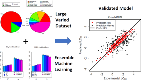
QSAR modeling can be used to aid testing prioritization of the thousands of chemical substances for which no ecological toxicity data is available. We drew on the U.S. Environmental Protection Agency’s ECOTOX database with additional data from ECHA to build a large data set containing in vivo test data on fish for thousands of chemical substances. This was used to create QSAR models to predict two types of endpoints: acute LC₅₀ (median lethal concentration) and points of departure similar to the NOEC (no observed effect concentration) for any duration (named the “LC₅₀” and “NOEC” models, respectively). These models used study covariates, such as species and exposure route, as features to facilitate the simultaneous use of varied data types. A novel method of substituting taxonomy groups for species dummy variables was introduced to maximize generalizability to different species. A stacked ensemble of three machine learning methods—random forest, gradient boosted trees, and support vector regression—was implemented to best make use of a large data set with many descriptors. The LC₅₀ and NOEC models predicted endpoints within one order of magnitude 81% and 76% of the time, respectively, and had RMSEs of roughly 0.83 and 0.98 log₁₀(mg/L), respectively. Benchmarks against the existing TEST and ECOSAR tools suggest improved prediction accuracy.

Graphical Abstract

Introduction

The Toxic Substances Control Act (TSCA) requires the US Environmental Protection Agency (EPA) to “compile, keep current and publish a list of each chemical substance that is manufactured or processed, including imports, in the United States for uses under TSCA.”¹ The TSCA Active Inventory² includes about 33,000 substances with around 400 new substances added every year, a pace that cannot be matched by in vivo toxicology studies alone. The Frank R. Lautenberg Chemical Safety for the 21st Century Act directs the EPA to reduce the use of vertebrate animal testing, instead making use of computational toxicology and bioinformatics approaches when scientifically justified³. To this end, a number of QSAR models have been developed for various mammalian toxicity endpoints, such as developmental toxicity⁴ or reproductive toxicity⁵, utilizing many strategies, such as deep learning⁶ or inclusion of study covariates.

Several QSAR models have been created specifically for aquatic toxicology. ECOSAR⁷ is a multispecies QSAR tool including models of acute and chronic lethal concentrations and points of departure created by the EPA. An independent study⁸ reported that ECOSAR’s acute LC₅₀ (median lethal concentration) fish predictions were correct within an order of magnitude (in mg/L) about 69% of the time on a set of industrial chemicals. The EPA’s TEST⁹ software includes a model that makes predictions for acute LC₅₀ in four-day fathead minnow studies; its authors reported an RMSE (root-mean-square-error) of 0.77 log₁₀(mol/L) and an R² (coefficient of determination) of 0.73. Singh et. al¹⁰ published the results of an ensemble tree learner model for four day LC₅₀ in Japanese medaka, reporting a maximum R² of 0.61 on 334 chemicals. Gramatica et. al¹¹ created a multiple linear regression based model for LC₅₀ in fathead minnows for 67 chemicals found in personal care products; they reported a Q² of 0.79 and a cross-validated RMSE of 0.63 log₁₀(mol/L).

One of the biggest challenges in QSAR modeling is correctly estimating model performance on new chemicals. Misleading error estimation can arise from using a favorable choice of validation set¹² or from statistical fluctuations, especially when the test set size is small. Differences in experimental conditions are another major obstacle, and many modelers have tried to account for this by limiting their training data to highly homogeneous sets^{7, 11, 13}. This improves model accuracy while shrinking the domain of applicability, limiting predictivity to those species, chemical groups, and experiment types where data is already abundant.

Our goal was to create robust multispecies fish toxicity QSAR models to guide testing prioritization. We incorporated as much experimental data as possible to create models with wide applicability domains that would exhibit high predictivity on new data, be less prone to overfitting, and yield a more precise estimate of their uncertainty. To deal with experimental and interspecies variability, these models include study covariates and a taxonomy-based accounting of species as parts of their feature sets. Two models have been built: one that predicts acute LC₅₀ and one that predicts repeat dose NOEC (no observed effect concentration), LOEC (lowest observed effect concentration), MATC (maximum acceptable toxicant concentration), and LC₀ (no observed lethal effect concentration). All reported concentrations and error statistics are given in log₁₀ transformed values (units of mg/L).

Materials and Methods

Data Acquisition and Cleaning

We began by downloading all of the ecotoxicity data from EPA’s ToxValDB¹⁴, a curated database that contained aquatic toxicity endpoints drawn from the ECOTOX and ECHA (European Chemicals Agency) databases. The current version of ToxValDB is accessible through the EPA’s CompTox Chemicals Dashboard¹⁵ (“CompTox”) (https://comptox.epa.gov/dashboard) and further information is given in Text S8. ECOTOX contributed 85,634 (89%) studies after cleaning, while ECHA contributed 10,226 (11%) studies. Each toxicity endpoint corresponded to one experimental study with the same covariates. The DSSTox¹⁶ library was used to match a DSSTox substance ID to each chemical according to its CAS Registry Number (CASRN); unmatched entries were discarded. Next, the ECOTOX website’s “Explore” function¹⁷ was used to match species scientific names in the ECHA data to common names in the ECOTOX data, as well as to prune non-fish species.

A substantial amount of cleaning was performed not only to standardize formatting, but also to trim away heterogeneous data types. Misspelled, uninformative, dissimilar or rare endpoint types were either standardized or discarded. LC endpoints were rounded to the nearest of LC₀, LC₂₅, LC₅₀, LC₇₅, or LC₁₀₀ (e.g. LC₁₀’s were grouped in with LC₀) while “EC₀” and “NOEL” endpoints were grouped with “NOEC”. Measurement units were standardized to units of log₁₀(mg/L) where feasible; otherwise, the entry was omitted. Exposure routes were standardized where possible, and only the major types were kept: “static”, “renewal”, and “flow-through”. A significant number of experiments had missing exposure routes and were relisted as “unreported”.

To match ECOTOX categorization, ECHA phenotypes were relabeled to study types “mortality”, “growth”, “reproductive”, “behavior”, “unreported”, or “multiple” by matching relevant keywords. Study durations for aquatic studies were converted to units of days when possible and otherwise omitted. Durations of fewer than seven days were assigned a duration class of “acute”, those longer than 28 days were labeled “chronic”, and those in between were labeled “subchronic”. This was done because fine-grained durations had a negligible predictive ability that was outweighed by the benefits of averaging multiple experiments of similar duration. Finally, experiments with an exposure method of “no substrate” or a study year of “19xx” were deleted. Overall, about 13% of the original studies were eliminated during the cleaning process (See Table S1 and Table S2).

Data Preparation

This data set was used to create two separate models: the “LC₅₀” model used only acute mortality studies for which an LC₅₀ was provided, while the “NOEC” model used endpoints similar to NOEC: NOEC, LOEC (lowest observed effect concentration), LC₀ (no observed lethal concentration), and MATC (maximum acceptable toxicant concentration). The endpoint type is treated as a kind of experimental covariate; this aggregation makes it easier for the model to extract the effects of chemical structure and other confounding variables while still ultimately accounting for the effect of endpoint type. Our design philosophy prioritized having a large amount of data over having a pure data set, based on the assumption that chemical structure is the principal driver of endpoint variation. Instead of limiting our training data by experiment type (e.g. using only fathead minnow studies) and leaving it to the user to decide whether those predictions might be extended to other situations, we incorporated all commonly available experimental setups explicitly and allowed the model to adjust its predictions accordingly.

Chemicals with incomplete chemical descriptors were discarded, primarily inorganics and mixtures. Stereoisomers and chemicals with the same desalted base were combined by matching chemicals with the same descriptor set. Only studies using species in the Actinopterygii class were kept. The final LC₅₀ data set contained 34,645 experiments performed using 2,656 unique chemicals on 358 species of fish (See Table S1). The NOEC data set, meanwhile, contained 14,484 experiments performed using 1,926 chemicals on 221 species of fish (See Table S2).

Chemical Descriptors

Chemical descriptors consisted of OPERA¹⁸ physiochemical properties and PaDEL descriptors¹⁹. OPERA is a free and open source suite of QSAR models based on PaDEL descriptors predicting physiochemical properties, (such as logP, vapor pressure, and water solubility) and environmental fate endpoints. The melting point was omitted because salt information has a significant impact on those predictions. OPERA predictions were downloaded from CompTox using DSSTox IDs.

The feature set was dominated by 1,444 PaDEL descriptors, the largest categories of which were the electrotopological states and autocorrelations; together these accounted for 835 descriptors. Other notable descriptors included the atom, ring, and bond counts, molecular weight, and various kinds of estimations for logP. For chemical structures, we used pre-curated QSAR-Ready²⁰ SMILES, which are publicly available on CompTox and described in more detail in Text S7.These were fed into a KNIME²¹ workflow that filtered out missing strings and converted the rest into Chemistry Development Kit²² .sdf formatting for increased compatibility with PaDEL. 1D and 2D PaDEL descriptors were generated from these files with the “detect aromaticity”, “remove salt”, and “standardize nitro groups” options checked (although these last two options would have no effect on QSAR-ready SMILES). PaDEL’s output contained a handful of non-numeric values, such as “Infinity”; chemicals containing these values were ultimately dropped from the data set. Logarithmic scaling was used to automatically scale any continuous, nonnegative chemical descriptors that spanned more than two orders of magnitude (See Text S1 for details). This could add a bias for descriptors near the threshold, but with thousands of descriptors, some spanning several orders of magnitude and some only one, this was judged to be the most principled method of discrimination. In practice, the scaling had a minimal effect on performance.

Experimental Covariates

Experimental covariates track potentially important study conditions. Those considered were: scientific species name, common species name, endpoint type, study type (e.g. growth, mortality), study duration class (e.g. acute, chronic), exposure route (e.g. static, renewal), exposure method (e.g. salt water, freshwater), study duration value, study phenotype (e.g. length, eggs hatched), study year, and data source. Truong et al.²³ showed that tracking these conditions at the study level can help disentangle the effects of the chemical from other factors. Only covariates expected to have a significant correlation with the endpoint were kept: species, duration class, study type, endpoint type, and exposure route (only species and exposure route were needed for the LC₅₀ model). Covariates were added to the model in the form of binary dummy variables representing each category, except in the case of species. The full taxonomy tree was downloaded from the NCBI taxonomy database²⁴ and a binary feature was created for every species, genus, family, etc. up to the largest common taxonomy group: Actinopterygii. The head of the taxonomy tree that remained after feature selection in the LC₅₀ model is shown in Figure S1. Adding taxonomy groups created a natural way to gauge experiment similarity, though there was no evidence of performance improvement versus using only the species and omitting higher taxonomy levels. Including descriptors from multiple taxonomic levels allowed experiments to be grouped at different scales according to how much data is available; the model can then choose the most useful descriptors automatically. The feature selection process described in the next section ensured that none of these descriptors were multicollinear or redundant and that they were each studied using a minimum number of chemicals.

Although our focus was modeling chronic endpoints in the NOEC model, other duration classes were included to improve predictivity. The NOEC model contained a significant number of studies with “unreported” exposure routes to bulk up its data set; conversely, these were left out of the LC₅₀ model to maintain its integrity. Study types were limited to either “mortality”, “growth” or “reproductive”.

Narcotic classifications were obtained using the OECD QSAR Toolbox (version 4.1) Verhaar classifications²⁵. Chemicals identified as belonging to class 1 and 2, polar and nonpolar narcotics, were together grouped under the “narcotic” designation and all other chemicals were designated “non-narcotic”. Similarly, we classified chemicals known to be estrogen receptor (ER) and androgen receptor (AR) agonist/antagonists to be “endocrine active” based on models incorporating multiple ER and AR assays²⁶. Those giving negative results were classified as “endocrine inactive”. These categories were used for performance analysis but were not part of the model.

Feature Selection

After data preparation, feature selection was performed using the training set. First, duplicated features, constant features, and binary features that varied in fewer than 14 unique chemicals were eliminated. This last step ensured with 95% certainty that a given feature would vary at least once in the test set. Features with a squared Pearson correlation of more than 0.8 with another feature were then removed one at a time, beginning with the feature with the most pairs, until no pairs remained; this removed about 600 features in each model. Although a significant number of features were removed in this process, the impact on predictivity was negligible and the computational time reduction significant. Features unlikely to be correlated with the endpoint were removed by performing a t-test with binary features and building a multiple linear regression with non-binary features, removing those with p-values above 0.5. Finally, any multicollinear columns within the entire set were removed. Ultimately, 552 and 495 descriptors remained in the LC₅₀ and NOEC models, respectively. Feature attrition throughout this process is outlined in Table S3 and Table S4.

Experiments with the same remaining features were merged into one experiment group, using the arithmetic mean as a representative endpoint. Experiment groups represent combinations of chemicals and covariates, so there are often multiple experiment groups corresponding to a single chemical. As an example of how the data are arranged in practice, a mockup of the first two rows of the NOEC model matrix is shown in Figure 1. Each row corresponds to one experiment group, here corresponding to the same chemical but different species, exposure route, and duration. Each experiment group is modeled separately then aggregated to provide a single prediction for each chemical.

Figure 1:

First two rows of the NOEC model matrix. (Note: Some covariates, such as the acute duration class and LC₀ endpoint, are encoded by leaving alternative covariates equal to zero.)

Machine Learning

Chemicals were randomly divided into fifths, one of which was immediately set aside as a test set. The remaining training set was then randomly split into five cross-validation folds. Splitting was performed by chemical, not experiment, so that each chemical was present in only one set/fold. Three different machine learning methods were used to build models: random forest (RF)²⁷, gradient boosted trees (GBT)²⁸, and (kernel based) support vector regression (SVR)²⁹. These base learners were implemented using the open source R packages ranger³⁰ (random forest), xgboost³¹ (gradient boosted trees), and liquidSVM³² (support vector regression). These methods were chosen for their individual ability to fit the data and for diversity of type. Each of the models used was resilient to large feature sets, requiring only minimal feature selection.

These three base learners were then stacked³³ using a multiple linear regression meta-learner. To do this, each base learner was used to make fivefold cross-validated predictions for the training set and then retrained on the full training set to obtain predictions for the test set. Cross-validated predictions became features in a new metadata training set, while external validation predictions became features in a new metadata test set. The final metadata set thus consisted of only three features: one for each base learner. The meta-learner was trained on the full set of cross-validated training set predictions, providing a weight for each base learner. Final test set predictions were generated by using these weights to take a weighted average of the three base learner test set predictions (i.e. the metalearner test set). Final cross-validated predictions were calculated similarly by using a weighted average of base learner cross-validated predictions with weights obtained by training a linear regression on the other folds.

We trained single untuned stacked models in addition to more time-intensive bootstrapped and tuned models. For clarity, the former will be referred to as the “fast” model, while the latter will be called the “full” model. For the fast model we used gamma = 5 and lambda = 1e-5 for SVR, 300 trees for RF, 25 boosting rounds for GBT, and the package defaults for all other hyperparameters. These parameters were chosen to be in the range of good results without attempting to methodically identify optimal values.

In the full model, hyperparameters for each individual method were chosen during an initial tuning phase using random search optimization³⁴. One hundred randomized combinations of hyperparameters were sampled from a predetermined range of values. The combination of hyperparameters yielding the lowest cross-validation error was saved and used during the bootstrapping phase. In the bootstrapping phase, a series of ensemble models were trained with randomized noise added and differing cross-validation splits. Noise was added by sampling study values from a normal distribution centered at the experimental mean with a standard deviation equal to the average standard deviation of experiment groups with ten or more entries. The resulting predictions were then averaged to give a bootstrapped prediction for each experiment group. A general outline of the modeling process is shown in Figure 2.

Figure 2:

Model algorithm flow chart

Error Estimation

To estimate error bounds, we relied on the root mean square error (RMSE):

$$\mathit{\text{RMSE}}=\sqrt{\frac{{\sum }_{i=1}^n{\left(y_i-\widehat{y_i}\right)}^2}{n}}$$ (1)

where n is the number of predictions, y_i is the i-th experimental value, and $\widehat{y_i}$ is the i-th prediction. To evaluate the scale-independent performance of each model we used Q² for cross-validation error:

$$Q^2=1-\frac{{\sum }_{i=1}^n{\left(y_i-\widehat{y_i}\right)}^2}{{\sum }_{i=1}^n{\left(y_i-\overline{y}\right)}^2}$$ (2)

where $\overline{y}$ is the average experimental value. Likewise, the coefficient of determination R² is used to evaluate test set error. R² and Q² can be understood as a comparison of the efficacy of the model versus the best constant model (i.e. the mean of experimental values). Since Todeschini et al.³⁵ pointed out that this measure can fluctuate based on the choice of test set, we always used the same test set when comparing two models’ performance. We also computed the standard deviation of the error:

$${\sigma }_E=\sqrt{\frac{{\sum }_{i=1}^n{\left(E_i-\overline{E}\right)}^2}{n-1}}$$ (3)

where E_i is the error of the i-th prediction $\left(y_i-\widehat{y_i}\right)$ and $\stackrel{-}{E}$ is the average error. For large n and $\overline{E}\approx 0$ (both of which hold in these models) σ_E ≈ RMSE. The benefit of calculating the standard deviation is that there is a well-known expression for calculating the upper and lower bounds of its 95% confidence interval:

$$s\sqrt{\frac{n-1}{{\chi }_{.975; n-1}^2}}\le {\sigma }_E\le s\sqrt{\frac{n-1}{{\chi }_{.025; n-1}^2}}$$ (4)

where s is the calculated standard deviation and χ² is the quantile function for the chi-squared distribution. Because σ_E ≈ RMSE, these intervals give an estimate on the bounds of a model’s RMSE based on the size of the test set. Thus, we can make conclusions about the significance of a difference in RMSE.

Benchmark Methodology

The TEST⁹ software includes a model (“TEST-LC₅₀”) that makes predictions for acute LC₅₀ but limits its scope to only fathead minnow tested over a span of four days in fresh water. TEST-LC₅₀ is a consensus model that averages the predictions of various clustering and regression-based models; its data set consists of 823 chemicals, one fifth of which were set aside for validation. For benchmarking, we chose three different test sets from chemicals not found in the TEST-LC₅₀ training set. A fast LC₅₀ model was retrained each time on all chemicals not present in the corresponding test set; other than the way the data was split into test and training sets, the model was the same as described in Machine Learning. The three test sets were:

1. Four-day FHM TEST-LC₅₀ test set: All chemicals in the TEST-LC₅₀ test set with LC₅₀ data matching the conditions (fathead minnow, four days, fresh water) required by TEST-LC₅₀.

2. Four-day FHM all chemicals: All chemicals outside the TEST-LC₅₀ training set with LC₅₀ data matching the conditions (fathead minnow, four days, fresh water) required by TEST-LC₅₀.

3. All acute, all fish, all chemicals: 523 (one-fifth of total chemicals) randomly chosen chemicals outside the TEST-LC₅₀ training set with acute LC₅₀ data for any species or exposure method.

ECOSAR⁷ uses an expert decision tree to categorize chemicals into one of 111 chemical classes, then uses a linear QSAR models based on log(K_OW) (octanol-water partition) to make predictions for both four day LC₅₀ and ChV values (equivalent to chronic MATC) for a generalized fish species. Multiple species were used to build ECOSAR’s models, with a focus on common test species, and the size of training sets varies between classes, from hundreds of chemicals to just one in some cases. We began by generating ECOSAR predictions for chemicals in our data set meeting the benchmark standards according to CAS registry number. Any chemicals that were desalted or missing from the ECOSAR database were omitted to avoid issues with different salt handling or SMILES formatting, along with any predictions that returned an alert or flag and any chemicals for which ECOSAR generated multiple predictions. As before, we retrained the appropriate fast model for each benchmark with the corresponding test set left out. Since ECOSAR training sets are laborious to extract from the documentation, they were not excluded from the LC₅₀ test set. Furthermore, a handful of ECOSAR training chemicals were kept confidential and could not be excluded from the MATC test sets. Three test sets were used:

1. LC₅₀: 523 (one-fifth of total chemicals) randomly chosen chemicals with freshwater, four-day LC₅₀ data that could be predicted by ECOSAR (ECOSAR’s training set was not omitted).

2. Chronic MATC: Chemicals outside ECOSAR’s fish ChV training set (when provided) with freshwater, chronic MATC data.

3. Expanded chronic MATC: Chemicals outside ECOSAR’s fish ChV training set (when provided) with freshwater, chronic MATC or NOEC and LOEC data, which were converted to MATC endpoints.

Software

ToxValDB was accessed August 2, 2018. Excel was used to remove dashes from and “Inf” values from PaDEL and CompTox output. KNIME (version 3.5.1) was used to reformat CompTox .sdf files to Chemistry Development Kit style .sdf files that could be used by PaDEL. PaDEL descriptors were calculated using PaDEL-Descriptor (version 2.21). All further data pre-preprocessing, model fitting, and validation steps were performed using R (version 3.4.4). ECOSAR predictions were obtained using ECOSAR (version 2.0). TEST-LC₅₀ predictions were accessed using the webTEST³⁶ service (TEST version 4.2.1, accessed August 2, 2018) accessed through CompTox. OPERA (version 1.5, accessed August 2, 2018) predictions were also accessed from CompTox.

Results and Discussion

Data Set

The data are not evenly distributed among species or chemicals (See Figure S2), the most common of which are listed in Table S5 and Table S6. While there is abundant data on some chemicals, 33% only have one entry in the LC₅₀ data, and 84% have ten or fewer entries. The distribution in the NOEC data is similar: 35% of chemicals have one entry and 85% have ten or fewer. The species distribution is likewise tilted toward a few preferred species, with rainbow trout, bluegills, and fathead minnows accounting for 43% and 50% of all studies in the LC₅₀ and NOEC data, respectively. The covariate makeup of each data set is shown in Figure S3, Figure S4, and Figure S5.

The LC₅₀ value distribution for the ten most common chemicals in the LC₅₀ data is plotted in Figure 3. Tightly clustered chemicals, such as Fenitrothion, still have an interquartile range spanning half an order of magnitude and dozens of outliers. Chemicals with more variance, like Malathion, can have interquartile ranges closer to 1.5 orders of magnitude. Dieldrin/Endrin is a case where there is a large cluster of outliers that appear to be due to a species-dependent effect. As another heuristic, the mean standard deviation of all chemicals with ten or more data points (468 in total) was 0.53 log₁₀(mg/L). The mean standard deviation of all experiment groups with ten or more data points (638 in total) was 0.41 log₁₀(mg/L). These values are intended to be a rough estimate of the noise inherent in the data; we would expect our predictive error RMSE to be larger than these values, but not by an overwhelming amount.

Figure 3:

Distribution of LC₅₀ values for the most common chemicals in the LC50 set. Asterisks indicates desalted and stereoisomer groups referred to by parent name.

Figure 4 shows the distributions for the most common chemicals in the NOEC set for each study duration class. Other confounding variables, such as species or endpoint type, remain lumped together. Some compounds vary little with duration class, while others show a significant decrease in median endpoint at longer durations (e.g. 2.4-Dinitrophenol). Even within duration classes, some chemicals, like Bisphenol A, can span nearly three orders of magnitude; however, other covariates may separate these distributions. The mean standard deviation of all chemicals with ten or more data points (319 in total) was 0.78 log₁₀(mg/L) and the mean standard deviation of all experiment groups with ten or more data points (105 in total) was 0.35 log₁₀(mg/L).

Figure 4:

Distribution of endpoints for the most common chemicals in the NOEC set. Asterisked names are desalted and stereoisomer groups referred to by parent name. Stars in the plot indicate p-value significance (* p<=.05, ** p<=.01, *** p<=.001) using the two sample Wilcoxon test versus the acute distribution.

Feature Importance

Although hundreds of features factored into each model, there were a small number possessing an outsized importance (see Figure S6). The top ten most important features in the RF and GBT base learners and LC₅₀ full model are presented in Table S7. Three OPERA predictions are prominent in both methods: water solubility, bioconcentration factor, and soil adsorption coefficient. The Ghose-Crippen prediction for octanol-water partition³⁷ is important in both learners, and the Broto-Moreau autocorrelation³⁸ shows up in each as well. The remaining features are all PaDEL descriptors, apart from the Otomorpha taxonomy group and static exposure route experimental covariates, each of which feature prominently in the gradient boosted trees learner.

Model Performance

In Table 1 we present error statistics for the LC₅₀ model. Q², R², RMSE, and σ_E are computed by comparing the average experimental value for a given chemical or experiment group to the average prediction for that chemical or experiment group. The last column shows the percentage of predictions correct within one order of magnitude. “CV” refers to the internal cross-validated predictions for one run, “EV” refers to predictions on the 20% of data that was set aside at the beginning, and “Combined” refers to both sets of predictions taken together. An external cross-validation was also performed on the fast model where each 20% of the original data was used as the EV set once (“External CV”). The first section gives the error statistics for the fast model, while the second and third repeat these for the full model aggregated by chemical and experiment group, respectively.

Table 1:

LC₅₀ model performance

	Validation Method	R2	Q2	RMSEi	σE lower	σEii	σE upper	Percent |Error| < 1
Fast model aggregated by chemical	CViii		0.59	0.84	0.81	0.84	0.86	80.9%
	EViv	0.58		0.81	0.76	0.80	0.85	81.6%
	Combined	0.59		0.84	0.81	0.83	0.85	81.1%
	External CV		0.59	0.83	0.81	0.83	0.85	80.9%
Full model aggregated by chemical	CV		0.60	0.83	0.80	0.82	0.85	81.5%
	EV	0.57		0.82	0.77	0.81	0.86	81.4%
	Combined	0.60		0.83	0.80	0.82	0.84	81.4%
Full model aggregated by experiment group	CV		0.64	0.91	0.90	0.91	0.93	77.2%
	EV	0.66		0.89	0.86	0.89	0.92	78.8%
	Combined	0.64		0.91	0.89	0.91	0.92	77.5

ⁱRMSE: Root-mean-square error

ⁱⁱσ_E : Standard deviation of error

ⁱⁱⁱCV: Cross-validation

^ivEV: External validation

Table 1 shows that the fast model had similar RMSEs and overlapping confidence intervals during EV and CV. The combined and external CV results are nearly the same, implying that the model has an Q² close to 0.59 and a RMSE near 0.83, significantly higher than the average standard deviation estimated in the Data Set section: 0.53. LC₅₀ is correctly predicted within one order of magnitude about 81% of the time. The bootstrapped model shows no improvement in the EV statistics and a small improvement in the CV statistics, suggesting that any improvement in combined error comes from overfitting due to tuning. The third section shows that the RMSEs are larger when the model is aggregated by experiment group instead of by chemical, though R² and Q² are larger as well. This may be because experiment groups are subsets of chemicals with fewer results in each; this implies there is more variability between endpoints, leading to a higher R², Q², and RMSE. Aggregating this way also skews the error towards that of the most studied chemicals.

The first three sections of Table 2 repeat these statistics for the NOEC model. The CV and EV RMSEs are roughly the same in the fast model and in the full model, though the full model again shows a slightly lower CV RMSE, probably due to overfitting during tuning. The NOEC model explains a little more of its variation than the LC₅₀ model with a Q² of 0.62, but the RMSE is significantly higher at 0.98. This RMSE is larger than the average standard deviation estimated in the Data Set section: 0.78. This can be explained by the relatively high variation of the NOEC data, relative to the more homogenous LC₅₀ set. Endpoints are correctly predicted within one order of magnitude about 76% of the time. The third section shows that the NOEC model also loses accuracy when aggregating by experiment group, though R² is unchanged. The fourth section shows the NOEC model’s performance for only chronic experiments. The chronic EV error is very high, but this appears to be a statistical anomaly, as the external CV error is similar to that of the regular fast model. This implies that there is no significant loss of performance for chronic studies.

Table 2:

NOEC model performance

	Validation Method	R2	Q2	RMSEi	σE lower	σEii	σE upper	Percent |Error| < 1
Fast model aggregated by chemical	CViii		0.60	1.00	0.95	0.98	1.02	74.3%
	EViv	0.59		1.01	0.93	1.00	1.07	76.4%
	Combined	0.60		1.00	0.96	0.99	1.02	74.7%
	External CV		0.62	0.98	0.94	0.97	1.00	75.8%
Full model aggregated by chemical	CV		0.63	0.96	0.92	0.95	0.99	75.3%
	EV	0.59		1.00	0.93	0.99	1.07	74.1%
	Combined	0.62		0.97	0.93	0.96	0.99	75.0%
Full model aggregated by experiment group	CV		0.63	1.09	1.07	1.09	1.10	69.1%
	EV	0.59		1.08	1.05	1.08	1.12	69.9%
	Combined	0.62		1.08	1.07	1.08	1.10	69.2%
Fast model chronic studies aggregated by chemical	CV		0.60	0.98	0.91	0.98	1.06	73.6%
	EV	0.33		1.20	1.05	1.20	1.41	61.5%
	Combined	0.55		1.03	0.96	1.03	1.11	71.0%
	External CV		0.57	1.01	0.94	1.01	1.08	71.2%

ⁱRMSE: Root-mean-square error

ⁱⁱσ_E : Standard deviation of error

ⁱⁱⁱCV: Cross-validation

^ivEV: External validation

Commonly studied modes of toxicity for fish and other ecological species are narcosis and endocrine disruption. Here we analyze how well the current model performs against chemicals known to act through these modes of action. When the narcotic classification was used as a feature, combined RMSE decreased by an insignificant amount, approximately .003 log₁₀(mg/L), in both the fast LC₅₀ and fast NOEC model. Table 3 shows the combined error for each of these chemical classes in the given (fast) model subset. In both models (LC₅₀ and NOEC), mortality endpoints for narcotic chemicals are significantly better predicted than those for non-narcotics, even in the absence of the explicit narcosis feature. Performance for growth and reproductive studies in endocrine active chemicals is not significantly different than performance in other chemicals. Figure 5 shows the related prediction error box plots for each of these categories. There is no obvious upward or downward shift for any of these categories. The total number of NOEC chemicals with endocrine-related data is 769 of the total 1926 (40%).

Table 3:

Performance for selected modes of action

Model	Method of Action	# Chemicals	R2	RMSE	σE lower	σE	σE upper	Percent |Error| < 1
LC50 All Studies	Narcotic	422	0.65	0.63	0.59	0.63	0.67	89.8%
	Non-narcotic	2234	0.57	0.87	0.84	0.86	0.89	79.4%
NOEC Mortality Studies	Narcotic	271	0.60	0.85	0.78	0.85	0.93	84.0%
	Non-narcotic	1655	0.58	1.01	0.97	1.00	1.04	72.3%
NOEC Growth & Reproductive Studies	Endocrine Active	110	0.16	1.03	0.89	1.03	1.23	71.6%
	Endocrine Inactive	659	0.59	1.02	0.93	1.02	1.11	74.7%

Figure 5:

Prediction errors for selected modes of action

Several other issues were explored in our analyses but did not change the overall results or conclusions. These are discussed in the supplemental material as follows: The model’s effectiveness at prioritization and the performance of individual base learners are discussed in Text S2 and accompanying figures. A brief discussion about health protective predictions is featured in Text S3. Further discussion of the error estimations resulting from bootstrapping are discussed in Text S4 and accompanying figures. Finally, the chemical space, applicability domain, and likely sources of error (activity cliffs³⁹, among them) are discussed in detail in Text S5 and accompanying figures.

Benchmark Results

Benchmarking results compared to TEST are given in Table 4. The first section of Table 4 suggests a moderate improvement with our model; however, the confidence intervals overlap, implying that the two models’ performance are not statistically separated with a benchmark this size. We hypothesize that any improvement in the first benchmark is primarily due to our larger training set, although adding taxonomic information probably contributed as well. In the second section both models perform significantly worse than before, signifying that this benchmark includes more challenging chemicals. The distance between the models’ performances has increased; now the confidence intervals barely overlap. Both models show their worst performance in terms of R² in the third benchmark; this can be explained by a difference in mean between training and test sets. With this larger test set the confidence intervals are much tighter and our model now shows a very significant increase in performance. The incorporation of many species in the third benchmark suggests that models based on a single species may not generalize very well to the entire fish population.

Table 4:

LC₅₀ external validation benchmark against TEST-LC₅₀.

	Model Used	Test Set Size	Train Set Size	R2	RMSEi	σE lower	σEii	σE upper	Percent |Error| < 1
Four-day FHM TEST-LC50 test set	TEST-LC50	141	659	0.61	0.74	0.67	0.75	0.84	83.7%
	Fast Model	141	2515	0.70	0.65	0.58	0.65	0.74	89.4%
Four-day FHM all chemicals	TEST-LC50	247	659	0.47	1.02	0.93	1.02	1.12	76.9%
	Fast Model	247	2409	0.63	0.86	0.79	0.86	0.94	79.4%
All acute, all fish, all chemicals	TEST-LC50	532	659	0.19	1.14	1.07	1.13	1.20	70.3%
	Fast Model	532	2124	0.58	0.81	0.76	0.81	0.86	81.4%

ⁱRMSE: Root-mean-square error

ⁱⁱσ_E: Standard deviation of error

Benchmarking results compared to ECOSAR are presented in Table 5. Our model performed much better than ECOSAR on the LC₅₀ benchmark with widely separated confidence intervals even with ECOSAR’s training set included. The models performed about the same on the second benchmark; however, the small sample size meant that the confidence intervals were wide and overlapping. The third benchmark saw both models decrease their performance, but while our model still performs reasonably well, ECOSAR performed very poorly, with a negative R². Though the test set size is still small, the confidence intervals no longer overlap in the third benchmark.

Table 5:

External validation benchmark against ECOSAR.

	Model Used	Test Set Size	Train Set Size	R2	RMSEi	σE lower	σEii	σE upper	Percent |Error| < 1
LC50	ECOSAR	532		0.23	1.07	1.01	1.07	1.14	83.6%
	Fast Model	532	2124	0.61	0.76	0.72	0.76	0.81	84.8%
Chronic MATC	ECOSAR	18		0.69	0.62	0.46	0.61	0.91	94.4%
	Fast Model	18	1908	0.78	0.52	0.40	0.54	0.80	94.4%
Expanded chronic MATC	ECOSAR	45		−0.60	1.50	1.24	1.50	1.89	66.7%
	Fast Model	45	1881	0.43	0.89	0.75	0.90	1.14	80.0%

ⁱRMSE: Root-mean-square error

ⁱⁱσ_E: Standard deviation of error

References

- 1.TSCA Chemical Substances Inventory. https://www.epa.gov/tsca-inventory/about-tsca-chemical-substance-inventory.
- 2.TSCA Active Inventory. https://www.epa.gov/tsca-inventory/how-access-tsca-inventory (accessed 6/6/2019).
- 3.Frank R, Lautenberg chemical safety for the 21st century act. Public Law 2016, (114–182). [Google Scholar]
- 4.Cassano A; Manganaro A; Martin T; Young D; Piclin N; Pintore M; Bigoni D; Benfenati E In CAESAR models for developmental toxicity, Chemistry Central Journal, Springer: 2010; p S4. [DOI] [PMC free article] [PubMed] [Google Scholar]
- 5.Novic M; Vracko M, QSAR models for reproductive toxicity and endocrine disruption activity. Molecules 2010, 15 (3), 1987–99. [DOI] [PMC free article] [PubMed] [Google Scholar]
- 6.Mayr A; Klambauer G; Unterthiner T; Hochreiter S, DeepTox: toxicity prediction using deep learning. Frontiers in Environmental Science 2016, 3, 80. [Google Scholar]
- 7.Mayo-Bean K; Moran K; Meylan B; Ranslow P, Methodology Document for the Ecological Structure-Activity Relationship Model (Ecosar) Class Program US-EPA: Washington DC: 2012. [Google Scholar]
- 8.Reuschenbach P; Silvani M; Dammann M; Warnecke D; Knacker T, ECOSAR model performance with a large test set of industrial chemicals. Chemosphere 2008, 71 (10), 1986–95. [DOI] [PubMed] [Google Scholar]
- 9.(a) Martin TM, User’s Guide for T.E.S.T. (version 4.2) (Toxicity Estimation Software Tool): A Program to Estimate Toxicity from Molecular Structure. EPA, U. S., 2016; [Google Scholar]; (b) Martin TM; Young DM, Prediction of the acute toxicity (96-h LC50) of organic compounds to the fathead minnow (Pimephales promelas) using a group contribution method. Chem Res Toxicol 2001, 14 (10), 1378–85. [DOI] [PubMed] [Google Scholar]
- 10.Singh KP; Gupta S; Kumar A; Mohan D, Multispecies QSAR modeling for predicting the aquatic toxicity of diverse organic chemicals for regulatory toxicology. Chem Res Toxicol 2014, 27 (5), 741–53. [DOI] [PubMed] [Google Scholar]
- 11.Gramatica P; Cassani S; Sangion A, Aquatic ecotoxicity of personal care products: QSAR models and ranking for prioritization and safer alternatives’ design. Green Chemistry 2016, 18 (16), 4393–4406. [Google Scholar]
- 12.Martin TM; Harten P; Young DM; Muratov EN; Golbraikh A; Zhu H; Tropsha A, Does rational selection of training and test sets improve the outcome of QSAR modeling? J Chem Inf Model 2012, 52 (10), 2570–8. [DOI] [PubMed] [Google Scholar]
- 13.Netzeva TI; Schultz TW, QSARs for the aquatic toxicity of aromatic aldehydes from Tetrahymena data. Chemosphere 2005, 61 (11), 1632–43. [DOI] [PubMed] [Google Scholar]
- 14.TOXVAL Database. US Environmental Protection Agency. [PubMed]
- 15.Williams AJ; Grulke CM; Edwards J; McEachran AD; Mansouri K; Baker NC; Patlewicz G; Shah I; Wambaugh JF; Judson RS, The CompTox Chemistry Dashboard: a community data resource for environmental chemistry. Journal of Cheminformatics 2017, 9 (1), 61. [DOI] [PMC free article] [PubMed] [Google Scholar]
- 16.(a) Richard AM; Williams CR, Distributed structure-searchable toxicity (DSSTox) public database network: a proposal. Mutation Research/Fundamental and Molecular Mechanisms of Mutagenesis 2002, 499 (1), 27–52; [DOI] [PubMed] [Google Scholar]; (b) Grulke CM; Williams AJ; Thillanadarajah I; Richard AM, EPA’s DSSTox database: History of development of a curated chemistry resource supporting computational toxicology research. Computational Toxicology 2019, 12, 100096. [DOI] [PMC free article] [PubMed] [Google Scholar]
- 17.ECOTOX Knowledgebase. https://cfpub.epa.gov/ecotox-new/explore.cfm (accessed 05/01/2018).
- 18.Mansouri K; Grulke CM; Judson RS; Williams AJ, OPERA models for predicting physicochemical properties and environmental fate endpoints. Journal of cheminformatics 2018, 10 (1), 10. [DOI] [PMC free article] [PubMed] [Google Scholar]
- 19.Yap CW, PaDEL‐descriptor: An open source software to calculate molecular descriptors and fingerprints. Journal of computational chemistry 2011, 32 (7), 1466–1474. [DOI] [PubMed] [Google Scholar]
- 20.(a) Mansouri K; Abdelaziz A; Rybacka A; Roncaglioni A; Tropsha A; Varnek A; Zakharov A; Worth A; Richard AM; Grulke CM; Trisciuzzi D; Fourches D; Horvath D; Benfenati E; Muratov E; Wedebye EB; Grisoni F; Mangiatordi GF; Incisivo GM; Hong H; Ng HW; Tetko IV; Balabin I; Kancherla J; Shen J; Burton J; Nicklaus M; Cassotti M; Nikolov NG; Nicolotti O; Andersson PL; Zang Q; Politi R; Beger RD; Todeschini R; Huang R; Farag S; Rosenberg SA; Slavov S; Hu X; Judson RS, CERAPP: Collaborative Estrogen Receptor Activity Prediction Project. Environmental Health Perspectives 2016, 124 (7), 1023–1033; [DOI] [PMC free article] [PubMed] [Google Scholar]; (b) Mansouri K; Grulke CM; Richard AM; Judson RS; Williams AJ, An automated curation procedure for addressing chemical errors and inconsistencies in public datasets used in QSAR modelling. SAR and QSAR in Environmental Research 2016, 27 (11), 911–937. [DOI] [PubMed] [Google Scholar]
- 21.Berthold MR; Cebron N; Dill F; Gabriel TR; Kötter T; Meinl T; Ohl P; Thiel K; Wiswedel B, KNIME-the Konstanz information miner: version 2.0 and beyond. AcM SIGKDD explorations Newsletter 2009, 11 (1), 26–31. [Google Scholar]
- 22.Steinbeck C; Han Y; Kuhn S; Horlacher O; Luttmann E; Willighagen E, The Chemistry Development Kit (CDK): An open-source Java library for chemo-and bioinformatics. Journal of chemical information and computer sciences 2003, 43 (2), 493–500. [DOI] [PMC free article] [PubMed] [Google Scholar]
- 23.Truong L; Ouedraogo G; Pham L; Clouzeau J; Loisel-Joubert S; Blanchet D; Nocairi H; Setzer W; Judson R; Grulke C; Mansouri K; Martin M, Predicting in vivo effect levels for repeat-dose systemic toxicity using chemical, biological, kinetic and study covariates. Arch Toxicol 2017. [DOI] [PMC free article] [PubMed] [Google Scholar]
- 24.Federhen S, The NCBI taxonomy database. Nucleic acids research 2011, 40 (D1), D136–D143. [DOI] [PMC free article] [PubMed] [Google Scholar]
- 25.Verhaar HJ; Van Leeuwen CJ; Hermens JL, Classifying environmental pollutants. Chemosphere 1992, 25 (4), 471–491. [DOI] [PubMed] [Google Scholar]
- 26.(a) Judson RS; Magpantay FM; Chickarmane V; Haskell C; Tania N; Taylor J; Xia M; Huang R; Rotroff DM; Filer DL, Integrated model of chemical perturbations of a biological pathway using 18 in vitro high-throughput screening assays for the estrogen receptor. Toxicological Sciences 2015, 148 (1), 137–154; [DOI] [PMC free article] [PubMed] [Google Scholar]; (b) Kleinstreuer NC; Ceger P; Watt ED; Martin M; Houck K; Browne P; Thomas RS; Casey WM; Dix DJ; Allen D; Sakamuru S; Xia M; Huang R; Judson R, Development and Validation of a Computational Model for Androgen Receptor Activity. Chem Res Toxicol 2017, 30 (4), 946–964. [DOI] [PMC free article] [PubMed] [Google Scholar]
- 27.Ho TK, The random subspace method for constructing decision forests. IEEE transactions on pattern analysis and machine intelligence 1998, 20 (8), 832–844. [Google Scholar]
- 28.Friedman JH, Greedy function approximation: a gradient boosting machine. Annals of statistics 2001, 1189–1232. [Google Scholar]
- 29.Drucker H; Burges CJ; Kaufman L; Smola AJ; Vapnik V In Support vector regression machines, Advances in neural information processing systems, 1997; pp 155–161. [Google Scholar]
- 30.(a) Wright MN; Ziegler A, ranger: A Fast Implementation of Random Forests for High Dimensional Data in C++ and R. 2017 2017, 77 (1), 17; [Google Scholar]; (b) Wright M. N. W., Stefan; Probst Philipp, ranger: A Fast Implementation of Random Forests. R Package version 0.9.0 2018. [Google Scholar]
- 31.(a) Chen T; Guestrin C In Xgboost: A scalable tree boosting system, Proceedings of the 22nd acm sigkdd international conference on knowledge discovery and data mining, ACM: 2016; pp 785–794; [Google Scholar]; (b) Chen T. H., Tong; Benesty Michael; Khotilovich Vadim; Tang Yuan, Xgboost: extreme gradient boosting. R package version 0.6.4.1 2018, 1–4. [Google Scholar]
- 32.(a) Steinwart I; Thomann P, liquidSVM: A fast and versatile SVM package. arXiv preprint arXiv:1702.06899 2017; [Google Scholar]; (b) Steinwart I. T., Philipp, liquidSVM: A Fast and Versatile SVM Package. R package version 1.2.1 2017. [Google Scholar]
- 33.(a) Wolpert DH, Stacked generalization. Neural networks 1992, 5 (2), 241–259; [Google Scholar]; (b) Witten IH; Frank E, Data Mining: Practical machine learning tools and techniques. Second ed.; Morgan Kaufmann: 2005. [Google Scholar]
- 34.Bergstra J; Bengio Y, Random search for hyper-parameter optimization. Journal of Machine Learning Research 2012, 13 (February), 281–305. [Google Scholar]
- 35.Todeschini R; Ballabio D; Grisoni F, Beware of Unreliable Q(2)! A Comparative Study of Regression Metrics for Predictivity Assessment of QSAR Models. J Chem Inf Model 2016, 56 (10), 1905–1913. [DOI] [PubMed] [Google Scholar]
- 36.Todd Martin AW, Valery Tkachenko In Prediction of toxicity and comparison of alternatives using WebTEST (Web-services Toxicity Estimation Software Tool) QSAR, Bled, Slovenia, June 11–15, 2018; Bled, Slovenia, 2018. [Google Scholar]
- 37.Ghose AK; Crippen GM, Atomic physicochemical parameters for three‐dimensional structure‐directed quantitative structure‐activity relationships I. Partition coefficients as a measure of hydrophobicity. Journal of computational chemistry 1986, 7 (4), 565–577. [Google Scholar]
- 38.Broto P; Moreau G; Vandycke C, Molecular structures: perception, autocorrelation descriptor and sar studies: system of atomic contributions for the calculation of the n-octanol/water partition coefficients. European journal of medicinal chemistry 1984, 19 (1), 71–78. [Google Scholar]
- 39.Cruz-Monteagudo M; Medina-Franco JL; Perez-Castillo Y; Nicolotti O; Cordeiro MND; Borges F, Activity cliffs in drug discovery: Dr Jekyll or Mr Hyde? Drug Discovery Today 2014, 19 (8), 1069–1080. [DOI] [PubMed] [Google Scholar]
Associated Data
This section collects any data citations, data availability statements, or supplementary materials included in this article.