Abstract
This work introduces a new software package “Sesame” for the numerical computation of classical semiconductor equations. It supports 1 and 2-dimensional systems and provides tools to easily implement extended defects such as grain boundaries or sample surfaces. Sesame is designed to facilitate fast exploration of the system parameter space and to visualize local charge transport properties. Sesame has been benchmarked against other software packages, and results for single crystal and polycrystalline CdS-CdTe heterojunctions are presented. Sesame is distributed as a Python package or as a standalone GUI application, and is available at https://pages.nist.gov/sesame/.
I. INTRODUCTION
Numerical simulations are an essential aspect of photovoltaic research and design. A number of free software packages have been developed and extensively used for solar cell modeling in 1-dimension, including AMPS [1], PC-1D [2], SCAPS [3], and wxAMPS [4]. Freely available 2-dimensional simulation tools are less common [5 7], but are necessary for describing systems with lateral inhomogeneity. A common class of such systems are polycrystalline thin film photovoltaics, such as CdTe [8], CIGS [9], and hybrid perovskites [10]. In these materials grain boundaries break the lateral symmetry of the p-n junction, leading to complex system geometries. Lateral inhomogeneity is also often encountered in nanoscale or mesoscopic measurements. The resolution of these measurements is typically achieved by using an excitation source or measurement probe with nanoscale spatial extent. Examples include electron beam induced current (EBIC) or scanning Kelvin probe microscopy, which are also often surface sensitive. An appropriate model for these measurements is therefore (at least) 2-dimensional and includes localized excitation/detection sources and relevant boundary conditions.
There are numerous examples of 2-dimensional solar cell modeling in the literature. For instance, the impact of grain boundaries in polycrystalline cells has been previously studied numerically [11–13] and analytically [14, 15]. Simulations have been used for interpreting experiments with localized excitations such as EBIC [16, 17], cathodololuminescence [18, 19], and two-photon photoluminescence [20]. Although these works are instructive, nonlinearities in the system response prevent a simple extrapolation of previous results to all possible system configurations of interest. Indeed there remain a number of unresolved questions of fundamental interest in polycrystalline photovoltaics, questions as basic as whether grain boundaries are harmful or beneficial to cell performance [8, 21]. It is therefore desirable for researchers to have widespread access to 2-d simulation software.
In this work we introduce Sesame, a Python package developed by the authors (B. G. and P. M. H.) which solves the drift-diffusion-Poisson equations in 1 and 2 dimensions. Sesame is open source and distributed under the BSD license. Sesame is designed to easily construct systems with planar defects, such as grain boundaries or sample surfaces, which may contain both discrete or a continuum of gap state defects. While full-featured commercial packages allow simulations of complex device configurations together with multiple physical effects, the needs of research sometimes require access to the source code and licensing that enables usage on computing clusters. Access to source code enables researchers to modify the program to suit their needs. The free licensing and Python implementation of Sesame allows batch processing of an arbitrary number of simultaneous simulations (limited only by cluster access). This provides the capacity for performing large scale parameter sweeps in multiple dimensions. The program and its code are publicly available at https://pages.nist.gov/sesame/.
The paper is organized as follows: In Sec. II we present a brief overview of the model and geometry. In Sec. III we compare the output of Sesame to established semiconductor modeling software, including SCAPS [3], Sentaurus [22], and COMSOL Semiconductor Module [23] [24]. In Sec. III we also present a hands-on tutorial script for solving a 2-dimensional system with a grain boundary, and briefly describe the functionality of the GUI. The mathematics underlying the model and technical details of the numerical implementation can be found in the Appendix.
II. OVERVIEW OF THE PHYSICAL MODEL
The system geometry consists of a semiconductor device connected to contacts at x = 0 mid x = L (see Fig. 1. Sesame describes the steady state behavior of this system, which is governed by the drift-diffusion-Poisson equations:
| (1) |
| (2) |
| (3) |
with the currents
| (4) |
| (5) |
where n and p are the respective electron and hole number densities, and φ is the electrostatic potential. is the charge current density of electrons (holes). Here, q is the absolute value of the electron charge, ρ is the local charge density, ϵ is the dielectric constant of the material, and ϵ0 is the permittivity of free space. μn,p is the electron/hole mobility, and is assumed to satisfy the Einstein relation: Dn,p = kBTμn,p/q. G is the electron/hole pair generation rate density and R is the recombination rate density.
FIG. 1.
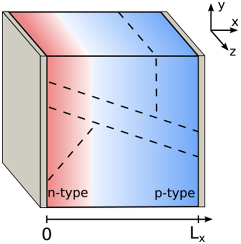
Coordinate system of Sesame: rectilinear geometry and contacts located at x = 0 and x = L. pn junction doping is shown as an example.
Sesame includes Schockley-Read-Hall, radiative, and Auger recombination mechanisms. Sesame is currently limited to describing non-degenerate semiconductors with Boltzmann statistics, and does not include thermionic emission and quantum tunneling at interfaces. These can be important contributions to the transport in heterojunctions [25], so care should be exercised when using Sesame to simulate such systems. Sesame includes Ohmic and Schottky contact boundary conditions, and periodic or hardwall (infinite potential) transverse boundary conditions. See Table I for a list of software capabilities and data output options. Note that Sesame currently does not include a solver for Maxwell’s equations. Sesame uses finite differences to solve Eqs. (1–3), and the standard Scharfetter-Gummel scheme for discretizing the current [26]. Details of the implementation can be found in the Appendix.
TABLE I.
List of features of Sesame (✓ indicates feature is available, ✗ indicates a feature is not available).
| Model features | |||
| Heterojunction | ✓ | Schottky contact | ✓ |
| Radiative/Auger recombination | ✓ | Schockley-Read-Hall recombination | ✓ |
| Graded material parameters | ✓ | Planar defects | ✓ |
| Thermionic emission | ✗ | Tunneling | ✗ |
| Boltzmann statistics | ✓ | Fermi-Dirac statatistics | ✗ |
| Time-dependent | ✗ | Scripting/batch processing | ✓ |
| Model output | |
| Spatially resolved electron/hole density | ✓ |
| Spatially resolved electron/hole current | ✓ |
| Surface (grain boundary) recombination | ✓ |
| Total recombination (defect, radiative, and Auger) | ✓ |
| J – V (Dark and light conditions) | ✓ |
III. BENCHMARKS AND EXAMPLES
A. Benchmarks
We first verify the consistency between Sesame and other software packages. We have compared the output of Sesame with the well-established software packages Sentaurus, COMSOL, and SCAPS for many systems, and present two illustrative examples here. We first consider a 1-d heterojunction consisting of a thin n+-doped layer of CdS and a p-type CdTe. The material parameters are shown in Table II. Fig 2(a) shows the computed J-V curve under a uniform generation rate density of G = 3.3 × 1020 cm−3 s−1. We find close agreement between Sesame, Sentaurus, and COMSOL. To quantify the comparison, we define the relative difference between two computed currents J1 and J2 as |J1 − J2|/〈J1 + J2〉, where 〈〉 denotes the average. The maximum relative difference between Sesame and Sentaurus is 0.2 %, and between Sesame and COMSOL it is 2 %. We observe a more substantial difference between Sesame and SCAPS, with a maximum value of 7 %. In all cases, the maximum discrepancy occurs near Voc, where the current is minimized so that relative differences are maximized. We attribute the larger difference between Sesame and SCAPS to the different interface recombination model used in SCAPS, in which the system variables are multi-valued at the interface and allow for recombination between layers [3].
TABLE II.
List of bulk parameters used for the 1-d and 2-d simulations. The label (D) and (A) for the doping value indicate donor and acceptor, respectively.
| Param. | CdS | CdTe |
|---|---|---|
| L [nm] | 25 | 4000 |
| ϵ | 10 | 9.4 |
| τn [ns] | 10 | 5 |
| τp [ns] | 10−4 | 5 |
| NC [cm−3] | 2.2 × 10¹⁸ | 8 × 10¹⁷ |
| NV [cm−3] | 1.8 × 10¹⁹ | 1.8 × 10¹⁹ |
| Eg [eV] | 2.4 | 1.5 |
| χ [eV] | 4.0 | 3.9 |
| μn [cm2/(V · s)] | 100 | 320 |
| μp [cm2/(V · s)] | 25 | 40 |
| doping [cm −3] | 1017 (D) | 1015 (A) |
FIG. 2.
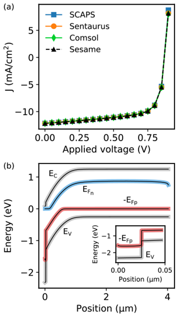
Comparison between Sesame and SCABS, Sentaurus, and COMSOL for a CdS-CdTe heterojunction, (a) Illuminated J-V curve. (b) Band diagram under short circuit conditions. Inset shows the valence band and hole quasi-Fermi level near the CdS layer. Black thin lines are the Sentaurus results, and thick colored lines are Sesame results.
We next, consider a 2-d system comprised of the same bulk materials, with a vertical grain boundary in the CdTe layer (see inset of Fig. 3(a)). The system width is 3 μm and we use hard wall boundary conditions for the vertical system edges. The grain boundary is positioned in the middle of the CdTe layer, and terminates a distance 0.1 μm from the p-type contact, and 25 nm away from the CdS interface. The grain boundary contains a discrete donor and acceptor defect, both positioned at 0.4 eV above midgap, with defect density ρGB = 1014 cm−2 electron capture cross section σGB = 10−14 cm2. For this simulation we again use a uniform generation rate G = 3.3 × 1021 cm−3 s−1. Fig. 3(a) shows the illuminated J-V curve obtained with Sesame, COMSOL, and Sentaurus (SCAPS is not included, as it does not support 2-d geometries). We again find good agreement between Sesame and the other software packages: the largest relative difference between Sesame and Sentaurus is 1.8 %, and between Sesame and COMSOL it is 0.7 %. Fig. 3(b) shows the good agreement obtained for the band diagram along the grain boundary core under short-circuit conditions for the three software packages.
FIG. 3.
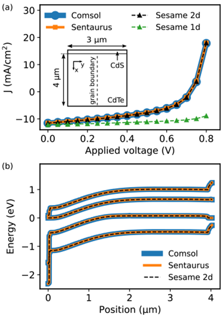
Comparison between Sesame, COMSOL and Sentaurus for a 2-dimensional system, (a) Illuminated JV curve. Inset: schematic of the system, an n-p junction with a columnar grain boundary, (b) Band diagram along the grain boundary core under short-circuit conditions.
In Fig. 3(a) we also include the J – V curve obtained with the 1-d simulation: the large difference between the 1-d and 2-d results reveals the crucial role the grain boundary plays in the system response. We’ve also checked that Sesame matches commercial software for systems with non-vertical, or “tilted” grain boundaries, and for system with multiple, intersecting grain boundaries [27]. Systems with complex grain boundary geometries are easily constructed in Sesame: the grain boundary endpoints are the only required input, and the software automatically embeds the planar defect in the real space mesh. The dependence of device behavior on grain boundary orientation and geometry was recently studied using Sesame in Ref. [28].
B. Scripting example
Sesame is run either through a self-contained GUI, or as a python package which is called in scripts. Running sesame with scripts is particularly convenient for running large-scale batch simulations on a computing cluster. Scripting also provides more flexibility in system definition (e.g. continuous grading of electronic parameters and doping). In the distribution, we provide several example scripts which describe standard PV simulations (e.g. J-V, IQE calculations), along with in-depth tutorials in the documentation. Here we give a description of a script to build and solve a simple 2-d simulation with a grain boundary.
We first import the numpy and sesame packages:
import sesame
import numpy as np
Next we define the grids for x and y. We use uniform grids for this example, but generally non-uniform grids are necessary to optimize the simulation accuracy and speed (non-uniform grids are used in the simulation of Fig. 3). (Note: Sesame assumes all lengths are given in units of cm.)
x = np.linspace(0,3e-4, 100)
y = np.linspace(0,3e-4, 100)
We create the system with the Builder function. The input to Builder are the x and y grids. The output is an object sys which contains all the information needed to describe the simulation.
sys = sesame.Builder(x, y)
Additional simulation settings are set by calling various methods of sys, as we show below.
Next we define the material properties with a python dictionary object (called mat in this example). The dictionary key names correspond to standard definitions. (Note: Sesame assumes times are given in units of s, energies in units of eV, densities in units of cm−3, mobility in units of cm/V · s)).
mat = {‘Nc’:8e17, ‘Nv’:1.8e19, ‘Eg’:1.5, ‘affinity’:4.1, ‘epsilon’:9.4, ‘Et’:0, ‘mu_e’:320, ‘mu_h’:40, ‘tau_e’:1e-8, ‘tau_h’:1e–8}
The dictionary key Et represents the energetic position of bulk recombination centers, as measured from the intrinsic energy level, and tau_e/tau_h are the electron/hole lifetimes. The dependence of the Schockloy-Road-Hall recombination on these parameters can be found in the Appendix. The material is added to the system using the add_material function, which takes the mat dictionary as input. Note that add_material is a method of the sys object, and is called with the command:
sys.add_material(mat)
To build a p-n junction we add a position-dependent doping profile to the system. We must define functions which describe the different doping regions: for this example, these functions are called n_region and p_region. They return True when the input variable position belongs to the region. For this example the two regions are delimited at the junction coordinate which corresponds to x = 10−5 cm.
junction = 1e–5
def n_region(position):
x, y = position
return x < junction
def p_region(position):
x, y = position
return x >= junction
Having defined the different doping regions, we add the donors and acceptors with the sys methods add_donor and add_acceptor. The input for these methods are the doping magnitude and doping region functions we just defined. Sesame currently assumes that all bulk dopants are fully ionized. (Note: Sesame assumes the units of density is cm−3):
donorDensity = 1e17
sys.add_donor(donorDensity, n_region)
acceptorDensity = 1e15
sys.add_acceptor(acceptorDensity, p_region)
Next we specify the contact boundary conditions. For this example, we specify Ohmic contacts with the function contact_type. Note the order of input arguments is left contact (x = 0) type first, right contact (x = L) type second:
sys.contact_type(‘Ohmic’,’Ohmic’)
We next specify the value of recombination velocity for electrons and holes at both contacts (Note: Sesame assumes the units of velocity are cm/s). For this example, both contacts only collect majority carriers. This is accomplished with the function contact_S:
Sn_L, Sp_L, Sn_R, Sp_R = 1e7, 0, 0, 1e7
sys.contact_S(Sn_L, Sp_L, Sn_R, Sp_R)
Next we add a grain boundary. We must specify the grain boundary defect energy level EGB (note the defect energy level is measured from the intrinsic energy level), the electron and hole capture cross sections sigmaeGB and sigmahGB, the defect density rhoGB, and the endpoints of the line defining the grain boundary p1, p2. These are input arguments to the function add_defects which creates a grain boundary. We also specify the charge transition states of the defect with the function input transition. In this case the specified charge states are (+1,−1), corresponding to having a donor and acceptor at the same energy level.
EGB =0.4
sigmaeGB = 1e–15
sigmahGB = 1e–15
rhoGB = 1e14
p1 = (.1e–4, 1.5e–4)
p2 = (2.9e–4, 1.5e–4)
sys.add_defects([p1, p2], rhoGB, sigmaeGB, sigmahGB, EGB, transition=(+1, −1))
We add illumination by defining a function illumination which returns the position-dependent intensity as a function of the input coordinate x,y
def illumination (x,y):
return 2.3e21 * np.exp(−2.3e4 * x)
sys.generation(illumination)
With the system now fully defined, we specify the list of applied voltages used to compute the current-voltage relation with the IVcurve function:
voltages = np.linspace(0,1,11)
jset = sesame.IVcurve(sys, voltages, ‘GB_JV’)
The function IVcurve returns an array jset containing the computed current density for each applied voltage. The IVcurve function also saves output files with seedname “GB_JV” concatenated with a suffix labeling the applied voltage index. These output files contain objects describing the simulation settings and the solution arrays. By default these files are compressed data files containing python Pickle objects (.gzip files). There is also an option to output the data in Matlab format (.mat files). Sesame includes an Analyzer object which contains several functions for computing quantities of interest from the solution, such as current densities, total recombination, carrier densities, and others. We refer the reader to the online documentation for a detailed list of all these functions.
C. GUI
Use of the standalone GUI as an alternative to scripting can be more convenient for small-scale calculations, or for those without access to a python distribution. Simulation settings can be saved and loaded, and the GUI also provides an interactive python prompt. The GUI is divided into three tabs, as shown in Fig. 4:
FIG. 4.
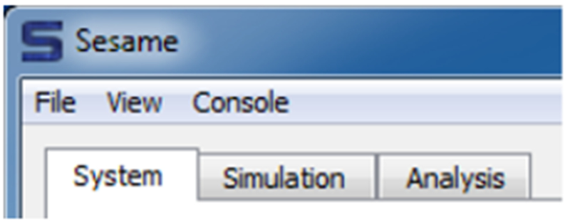
Menu and 3 main tabs of the Sesame GUI. See text for a description of the functionality of each tab.
1. The System tab contains fields to define the system geometry and material parameters (see Fig. 5).
FIG. 5.
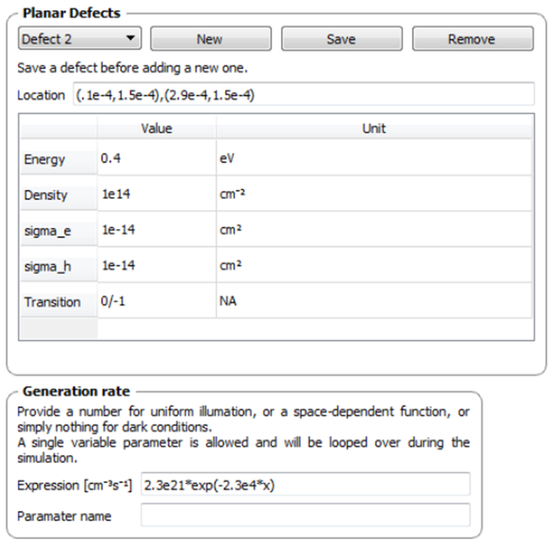
Panels from System tab of the GUI. In the planar defects panel, an arbitrary number of planar defects can be defined by specifying the endpoints of the boundary (a 1-d line for a 2-dimensional simulation), the defect energy, density, electron and hole capture cross sections, and charge states. The Generation rate panel allows for one user-defined parameter to be varied.
2. The Simulation tab lets the user specify which parameter is varied: either the voltage is swept, or a user-defined variable related to the generation rate density is swept. The boundary conditions and output file information is also set here, and the simulation is launched from this tab. The program output is provided so that the user can follow the progress of the calculations.
3. The Analysis tab enables the user to plot the output of the simulation, and to save and export plotted data (see Figs. 6 and 7).
FIG. 6.
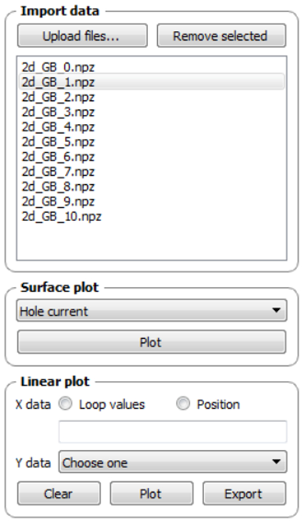
Panel from Analysis tab of the GUI. Data files can be selected for analysis, and surface plots of system variables and observables can be generated for 2-dimensional systems. A linear plot with two modes is available. In “loop values” mode, a scalar (such as total current) is plotted versus the looped parameters. In the “position” mode, a system variable or observable from a single solution is plotted versus spatial coordinate.
FIG. 7.
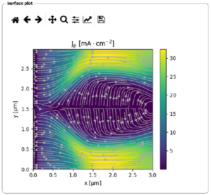
The surface plot panel of the Analysis tab of the GUI. This shows the hole currents flowing in a homojunction with a single grain boundary.
Sesame is distributed with a number of sample input files for setting up standard PV simulations in the GUI. More detailed documentation for the GUI is included in the distribution.
IV. CONCLUSION
Modeling tools are essential for describing and understanding polycrystalline materials and nanoscale measurements. System behavior for complex, 2-dimensional geometries can be drastically different than the textbook 1-dimensional p-n junction model. Numerical simulations provide the capability to explore and develop intuition about this rather unchartered territory. Our aim in releasing Sesame is to provide the research community with a free, easy-to-use resource which will enable broader use of simulation in complex photovoltaic systems. There are opportunities for additional functionalities (e.g. time-dependence, small-signal analysis, more advanced interface transport models) and further optimizations (e.g. use of Cython) of the code. Our intent in releasing the fully documented source code is to provide users the option to make these and other additions as their research needs require. An additional feature not discussed here is 3-dimensional modeling, which is included in the distribution as an untested feature which will be investigated further in future work.
ACKNOWLEDGMENTS
B. G. acknowledges support under the Cooperative Research Agreement between the University of Maryland and the National Institute of Standards and Technology Center for Nanoscale Science and Technology, Award 70NANB14H209, through the University of Maryland. Y. S. and P. B. acknowledge Support provided by the Department of Energy, under DOE Cooperative Agreement No. DE-EE0004946 (PVMI Bay Area PV Consortium), and the National Science Foundation Award EEC 1454315 CAREER: Thermophotonics for Efficient Harvesting of Waste Heat as Electricity. We thank Marc Burgelman for helpful correspondence, and thank Mike Scarpulla and Heayoung Yoon for helpful feedback on the software design. We thank Nick Rohrman for assistance in code development.
Appendix A. MODEL DETAILS
A. Mathematical Description
In this section we provide a full description of the equations solved by Sesame. These are fairly standard and can be found in textbooks [29–32], but we include them here for the sake of completeness and to specify notation and conventions used in the code. We first write densities in terms of quasi-Fermi levels, denoted by EFn and EFp for electrons and holes, respectively. Since we assume Boltzmann statistics (i.e. a non-degenerate semiconductor), the carrier densities are related to quasi-Fermi levels by:
| (6) |
| (7) |
where Eg is the material band gap, χ is the electron affinity, and NC,V are the conduction, valence band effective density of states, respectively. All quantities except temperature can vary with position.
The electron and hole current can be expressed in terms of the spatial gradient of the quasi-Fermi levels [33]:
| (8) |
| (9) |
1. Recombination
Sesame includes Shockley-Read-Hall, radiative and Auger recombination. The steady-state Shockley-Read-Hall recombination rate density is given by:
| (10) |
FIG. 8.
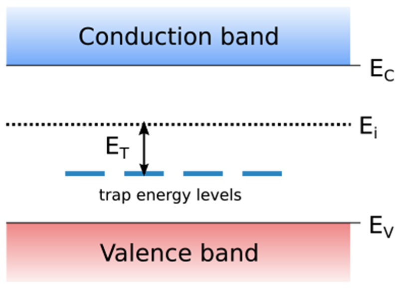
Depiction of energy levels of defect states. The intrinsic energy level is Ei = Eg/2 − kBT/q ln (NC/NV) as measured from the valence band edge.
where ni is the material intrinsic carrier density, given by . The equilibrium Fermi energy at which n = p = ni is the instrinsic energy level Ei. We specify the defect energy level ET relative to Ei (see Fig. 8), so that the expressions for n1 and p1 in Eq. 10 are given by:
| (11) |
| (12) |
τn,(p) is the bulk lifetime for electrons, holes. It is given by
| (13) |
where NT is the three-dimensional trap density, is the thermal velocity of carriers ( with mn,p the electron/hole effetive mass), and σn,p is the capture cross-section for electrons, holes.
The radiative recombination has the form
| (14) |
where B is the radiative recombination coefficient of the material. The Auger mechanism has the form
| (15) |
where Cn (Cp) is the electron (hole) Auger coefficient.
2. Planar defects
Sesame has been created with the intent of studying extended defects in solar cells, such as grain boundaries and sample surfaces. These extended planar defects are represented by a point in a 1-d model, a line in a 2-d model, and a plane in a 3-d model. The extended defect energy level spectrum can be discrete or continuous. For a discrete spectrum, we label the defect with the subscript d. The occupancy of the defect level fd is given by [34]
| (16) |
where n (p) is the electron (hole) density at the spatial location of the defect, Sn, Sp are recombination velocityparameters for electrons and holes respectively. nd and pd are
| (17) |
| (18) |
where Ed is calculated from the intrinsic level Ei.
The electron/hole recombination velocity are related to the electron/hole capture cross section and the defect density ρd according to:
| (19) |
The defect recombination is of Shockley-Read-Hall form:
| (20) |
The charge density given of a single defect depends on the defect type (acceptor vs. donor)
| (21) |
where ρd is the defect density of state at energy Ed. Multiple defects are described by summing over defect label d, or performing an integral over a continuous defect spectrum.
B. Boundary conditions at the contacts
For a given system definition, Sesame first solves the equilibrium problem. In equilibrium, the quasi-Fermi level of electrons and holes levels are equal and spatially constant. We choose an energy reference such that in equilibrium, EFp = EFn = 0. The equilibrium problem is therefore reduced to a single variable ϕeq (r). Sesame employs both Dirichlet and von Neumann equilibrium boundary conditions for ϕeq, which we discuss next.
1. System in thermal equilibrium
Sesame uses Dirichlet boundary conditions as the default. This is the appropriate choice apply when the equilibrium charge density at the contacts is known a priori. This applies for Ohmic and ideal Schottky contacts. For Ohmic boundary conditions, the carrier density is assumed to be equal and opposite to the ionized dopant density at the contact. For an n-type contact with ND ionized donors at the x = 0 contact (i.e. no free excess carriers at the contact), Eq. 6 yields the expression for ϕeq(x = 0):
| (22) |
Similar reasoning yields expressions for qϕeq for p-type doping and at the x = L contact.
For Schottky contacts, we assume that the Fermi level at the contact is equal to the Fermi level of the metal. This implies that the equilibrium electron density is NC exp [− (ΦM − χ)/kBT], where ΦM is the work function of the metal contact. Eq. 6 then yields the expression for ϕeq (shown here for the x = 0 contact):
| (23) |
An identical expression applies for the x = L contact.
Sesame also has an option for von Neumann boundary conditions, where it’s assumed that the electrostatic field at the contact vanishes:
| (24) |
The equilibrium potential ϕeq determines the equilibrium densities neq, peq according to Eqs. 6 and 7 with EFn = EFp = 0.
2. System out of thermal equilibrium
Out of thermal equilibrium, Dirichlet boundary conditions are imposed on the electrostatic potential. For example, in the presence of an applied bias V at x = L, the boundary conditions are
| (25) |
| (26) |
where ϕeq is the equilibrium electrostatic potential.
For the drift-diffusion equations, the boundary conditions for carriers at charge-collecting contacts are parameterized with the surface recombination velocities for electrons and holes at the contacts, denoted respectively by Scn and Scp :
| (27) |
| (28) |
| (29) |
| (30) |
C. Numerical implementation
In this section we review the set of equations solved by Sesame and provide some details of their implementation in the one-dimensional case.
1. Scharfetter-Gummel scheme
Sesame uses finite differences to solve the drift-diffusion-Poisson equations on a nonuniform grid. Fig. 9 shows our index-labeling convention for sites and links: link i connects site i and site i+1. Site-defined quantities (such as density and electrostatic potential) are labeled with a subscript denoting the site number. Link-defined quantities (such as electrical current and electric field) are labeled with a superscript denoting the link number.
We consider a one-dimensional system to illustrate the model discretization. First, we rewrite the current on link i in semi-discretized form:
| (31) |
| (32) |
A key step to ensure numerical stability is to integrate Eqs. (31) and (32) in order to get a completely discretized version of the current . This discretization is known as the Scharfetter-Gummel scheme [26]. Here we give the final expressions for the hole current between sites i and i + 1:
| (33) |
where ψp = qϕ + χ + Eg − kBT ln(NV) is the effective potential. The electron current is given by:
| (34) |
where ψn = qϕ + χ + kBT ln(NC).
In the limit where either δψn(p) ≡ −q(ψn(p),i+1 − ψn(p),i)/kBT or δEFn(p) ≡ (EFn(p),i+1 − EFn(p),i+1)/kBT are smaller than 10−5
FIG. 9.

Sites and links of the grid used in the discretization of the drift diffusion and Poisson equations.
TABLE III.
Quantities used to scale variables to dimension-less form.
| Quantity | Expression | Value |
|---|---|---|
| Density | N0 | 1019 cm−3 |
| Mobility | μ0 | 1 cm2/(V · s) |
| Temperature | T0 | 300 K |
| Energy | kBT0 | 0.0258 eV |
| Length (x0) | 3.78 × 10⁻⁸ cm | |
| Time | ϵ0/(qμ0N0) | 5.5 × 10⁻⁴ s |
| Gen. rate density | 1.81 × 1032 1/(cm3 · s) | |
| Current | μ0N0kBT/x0 | 1.10 × 10⁶ A/cm2 |
and 10−9, respectively, we replace the expressions for the current with a Taylor series expansion of the small parameter. In the expansion, we evaluate the current up to second order in δψn(p), and up to first order in δEFn(p).
Embedding a two-dimensional density into the three-dimensional model is formally accomplished with the use of a delta function. Numerically, the two-dimensional defect densities of states and the surface recombination velocities are divided by the size of the discretized grid at the position of the plane, and along the direction normal to the plane.
2. Newton-Raphson algorithm
The discretization of Eqs. (1)–(3) leads to the system of three equations for all sites of the discretized space (except boundary sites):
| (35) |
| (36) |
| (37) |
Because we exchanged the carrier densities for the quasi-Fermi levels as the unknowns of the problem, we are therefore looking for the sets EFn, EFp, ϕ at every grid point.
We use the Newton-Raphson method to solve the above set of equations: Given a general nonlinear function f(x), we want to find its root . Given x1 δx guess, assuming that the function varies linearly all the way to its root
| (38) |
An updated guess is provided by x2 = x1 − δx. The assumption of linear variation is key here, as if the guess x1 is too far from the root, the convergence of the algorithm is very uncertain.
In multiple dimensions the derivative in Eq. (38) is replaced by the Jacobian. In this case, Eq. (38) is a matrix equation of the form
| (39) |
where F is a vector function of the unknowns of the problem on all sites of the discretized space, and A is the Jacobian matrix given by
| (40) |
We find that convergence of the Newton-Raphson algorithm for this problem requires exact (analytically computed) values for the Jacobian.
In case the guess is far from the root we are looking for, the correction given by Eq. 38 can overshoot the solution. A simple way to improve the convergence is to damp the corrections δx given by Eq. (39). Inspired by an earlier work [35], we found that the following procedure gives good results. For δxi > 1, we replace δxi by
| (41) |
Contributor Information
Benoit Gaury, Center for Nanoscale Science and Technology, National Institute of Standards and Technology, Gaithersburg, MD 20899, USA and Maryland Nano Center, University of Maryland, College Park, MD 20742, USA.
Yubo Sun, School of Electrical & Computer Engineering, Purdue University, West Lafayette, IN, 47907, USA.
Peter Bermel, School of Electrical & Computer Engineering, Purdue University, West Lafayette, IN, 47907, USA.
Paul M. Haney, Center for Nanoscale Science and Technology, National Institute of Standards and Technology, Gaithersburg, MD 20899, USA
References
- [1].Zhu H, Kalkan AK, Hou J, and Fonash SJ, in AIP Conference Proceedings. Vol. 462 (AIP, 1999) pp. 309 [Google Scholar]
- [2].Basore PA and Clugston DA, in Photovoltaic Specialsts Conference, 1996., Conference Record of the Twenty Fifth IEEE (IEEE, 1996) pp. 377–381. [Google Scholar]
- [3].Burgelman M, Nollet P, and Degrave S, Thin Solid Films 361, 527 (2000). [Google Scholar]
- [4].Liu Y, Sun Y, and Rockett A, Solar Energy Materials and Solar Cells 98, 124 (2012). [Google Scholar]
- [5].Gray JL, in Photovoltaic Specialists Conference, 1991., Conference Record of the Twenty Second IEEE (IEEE, 1991) pp. 436–438. [Google Scholar]
- [6].Altermatt PP, Journal of computational electronics 10, 314 (2011). [Google Scholar]
- [7].Basore PA and Cabanas-Holmen K, IEEE Journal of Photovoltaics 1, 72 (2011). [Google Scholar]
- [8].Major JD, Semiconductor Science and Technology 31, 093001 (2016). [Google Scholar]
- [9].Yan Y, Noufi R, and Al-Jassim M, Physical review letters 96, 205501 (2006). [DOI] [PubMed] [Google Scholar]
- [10].Yun JS, Ho-Baillie A, Huang S, Woo SH, Heo Y,Seidel J, Huang F, Cheng Y-B, and Green MA, The journal of physical chemistry letters 6, 875 (2015). [DOI] [PubMed] [Google Scholar]
- [11].Edmiston S, Heiser G, Sproul A, and Green M, Journal of applied physics 80, 6783 (1996). [Google Scholar]
- [12].Gloeckler M, Sites JR, and Metzger WK, Journal of applied physics 98, 113704 (2005). [Google Scholar]
- [13].Rau U, Taretto K, and Siebentritt S, Applied Physics A 96, 221 (2009). [Google Scholar]
- [14].Gaury B and Haney PM, Journal of applied physics 120, 234503 (2016). [DOI] [PMC free article] [PubMed] [Google Scholar]
- [15].Gaury B and Haney PM, Physical Review Applied 8, 054026 (2017). [Google Scholar]
- [16].Haney PM, Yoon HP, Gaury B, and Zhitenev NB, Journal of applied physics 120, 095702 (2016). [DOI] [PMC free article] [PubMed] [Google Scholar]
- [17].Jin Y and Dunham ST, IEEE Journal of Photovoltaics 7, 329 (2017). [Google Scholar]
- [18].Kanevce A, Moseley J, Al-Jassim M, and Metzger WK, IEEE Journal of Photovoltaics 5, 1722 (2015). [Google Scholar]
- [19].Mendis B, Howkins A, Stowe D, Major J, and Durose K, Ultramicroscopy 167, 31 (2016). [DOI] [PubMed] [Google Scholar]
- [20].Kanevce A, Levi D, and Kuciauskas D, Progress in Photovoltaics: Research and Applications 22, 1138 (2014). [Google Scholar]
- [21].Kumar SG and Rao KK, Energy & Environmental Science 7, 45 (2014). [Google Scholar]
- [22].Guide SDU and Version E, Mountain View, CA, USA: (2013). [Google Scholar]
- [23].Multiphysics C, COMSOL AB, Stockholm, Sweden: (2017). [Google Scholar]
- [24].The full description of the procedures used in this paper requires the identification of certain commercial products. The inclusion of such information should in no way be construed as indicating that such products are endorsed by NIST or are recommended by NIST or that they are necessarily the best software for the purposes described.
- [25].Horio K and Yanai H, IEEE transactions on electron devices 37, 1093 (1990). [Google Scholar]
- [26].Gummel HK, IEEE Trans. Electron Devices 11, 455 (1964). [Google Scholar]
- [27].Gaury B, Sun Y, Bermel P, and Haney P, in 2018 IEEE 7th, World Conference on Photovoltaic Energy Conversion (WCPEC)(A Joint Conference of 45th IEEE PVSC, 28th, PVSEC & Sfth EU PVSEC) (IEEE, 2018) pp. 1882–1885. [Google Scholar]
- [28].Gaury B and Haney PM, ACS Applied Energy Materials 2, 144 (2018). [Google Scholar]
- [29].Pierret RF, Semiconductor device fundamentals (Pearson Education; India, 1996). [Google Scholar]
- [30].Fonash SJ, Solar cell device physics (Academic Press, 1981). [Google Scholar]
- [31].Selberherr S, Analysis and simulation of semiconductor devices (Springer Science & Business Media, 2012). [Google Scholar]
- [32].Vasileska D, Goodnick SM, and Klimeck G, Computational Electronics: semiclassical and quantum device modeling and simulation (CRC press, 2017). [Google Scholar]
- [33].Van Vliet KM and Marshak AH, Solid-State Electronics 23, 49 (1980). [Google Scholar]
- [34].Shockley W and Read WT, Phys. Rev 87, 835 (1952). [Google Scholar]
- [35].Brown G and Lindsay B, Solid-State Electronics 19, 991 (1976). [Google Scholar]


