Comprehensive Exploration of Target‐specific Ligands Using a Graph Convolution Neural Network

Abstract

Machine learning approaches are widely used to evaluate ligand activities of chemical compounds toward potential target proteins. Especially, exploration of highly selective ligands is important for the development of new drugs with higher safety. One difficulty in constructing well‐performing model predicting such a ligand activity is the absence of data on true negative ligand‐protein interactions. In other words, in many cases we can access to plenty of information on ligands that bind to specific protein, but less or almost no information showing that compounds don't bind to proteins of interest. In this paper, we suggested an approach to comprehensively explore candidates for ligands specifically targeting toward proteins without using information on the true negative interaction. The approach consists of 4 steps: 1) constructing a model that distinguishes ligands for the target proteins of interest from those targeting proteins that cause off‐target effects, by using graph convolution neural network (GCNN); 2) extracting feature vectors after convolution/pooling processes and mapping their principal components in two dimensions; 3) specifying regions with higher density for two ligand groups through kernel density estimation; and 4) investigating the distribution of compounds for exploration on the density map using the same classifier and decomposer. If compounds for exploration are located in higher‐density regions of ligand compounds, these compounds can be regarded as having relatively high binding affinity to the major target or off‐target proteins compared with other compounds. We applied the approach to the exploration of ligands for β‐site amyloid precursor protein [APP]‐cleaving enzyme 1 (BACE1), a major target for Alzheimer Disease (AD), with less off‐target effect toward cathepsin D. We demonstrated that the density region of BACE1 and cathepsin D ligands are well‐divided, and a group of natural compounds as a target for exploration of new drug candidates also has significantly different distribution on the density map.

1. Introduction

Current machine learning approaches using sophisticated methodologies and advanced computational techniques are highly developed. In cheminformatics, various applications of machine learning have been proposed for the construction of useful models to predict the chemical properties of compounds. One fascinating challenge is the prediction of the binding specificity of compounds to specific proteins. Such research is highly beneficial for the field of drug discovery, as many new drug candidates are withdrawn from nonclinical or clinical trials because of safety issues. One major cause of such safety issues is the nonspecific interaction of the drug with proteins other than the treatment target, i. e., off‐target effects. One example of such off‐target effects has been observed during the development of drugs to treat Alzheimer's disease (AD), the most common type of dementia, which causes neurocognitive disorders such as memory loss and loss of thinking ability. In AD, β‐secretase (β‐site amyloid precursor protein [APP]‐cleaving enzyme 1, abbreviated as BACE1) is considered a possible target for treatment.1 BACE1 is an enzyme that initiates the synthesis of amyloid β peptides (Aβ), a cause of AD. Although BACE1 inhibitors have been investigated, and some have been the subject of clinical trials, none has yet received approval from Food and Drug Administration. Safety concerns seem to be a major cause of these withdrawals, and some BACE1 inhibitors have been found to have ocular toxicity in preclinical animal models. The mechanism of this toxicity had been unclear, but a recent study implied that cathepsin D is an off‐target ligand of some BACE1 inhibitors, and that this undesirable binding is the cause of ocular toxicity.2 Therefore, improving the specificity of drugs for the target protein is a key factor in drug development. Quantum chemistry allows the quantitative prediction of a drug's binding affinity for a target protein, but requires a huge number of calculations, which imposes a large time and cost burden. Moreover, this approach requires high‐resolution information about the three‐dimensional (3D) structure of the target protein. A majority of targets is membrane proteins, and obtaining information about the 3D structure of membrane proteins is challenging because of technical difficulties in their crystallization. By contrast, a machine‐learning approach does not necessarily require information about the 3D structure of target proteins, provided that information is available about whether and/or how strongly each ligand binds to the target protein. By taking these factors into consideration, machine‐learning techniques make it possible to predict the binding specificity of ligand compounds.

When applying machine‐learning methods to chemical compounds, a major interest is how to extract the compound features and process them as vectors. One traditional way to do this is to construct vectors using molecular properties such as molecular weight, the number of atoms, octanol/water partition coefficient called logP, and polar surface area. However, model construction using such molecular properties does not always result in better predictive ability. As an alternative, researchers have investigated the extraction of structural properties directly from chemical structures, i. e., chemical fingerprints, to evaluate the existence of structural fragments. There are various types of chemical fingerprints depending on divergent definitions of structural fragments of interest (e. g., circular fingerprints [CF]). Using fingerprints as descriptors of ligands, machine learning can be applied to classify compounds or predict their properties (e. g., a neural network using fingerprinting dramatically improved performance for predicting quantitative structure–activity relationships3). Moreover, the use of graph theory for highlighting chemical structures using a graph convolutional neural network (GCNN) has been suggested. GCNNs enable the direct incorporation of the overall structural features of the compounds as input data, as in image processing. Compared with other machine‐learning methods, GCNNs have shown a better ability to predict drug absorption, distribution, metabolism and excretion (ADME) based on the chemical structure4, 5 and binding affinity of ligand compounds to specific target proteins.6 Similar to image processing, GCNNs consist of feature extraction layers, i. e., convolution and pooling layers and fully connected layers for classification/regression. Input data as graphs pass through the feature extraction layers, which results in decomposition of the vector dimensions used in fully connected layers. GCNNs seem to allow more efficient featurization, and perform well compared with chemical fingerprints such as CF.

To construct a classification model for the exploration of ligand candidates with higher specificity, it is not sufficient to prepare datasets for groups of selective and nonselective ligands, because the compounds used for exploration must be neither selective nor nonselective ligands; datasets for “nonligands” are also needed to allow construction of classification models that distinguish them from selective and nonselective ligands. In many cases, we can obtain plenty of information about ligands that bind to the target proteins of interest, but little or almost no information about ligands that do not bind to the proteins; i. e., true negative ligand–protein interactions are missing. To avoid this problem, ligands for entirely different proteins can be used as negatives, but even these ligands may have some binding affinity for the proteins of interest. Considering these factors, we proposed the development of a methodology using a GCNN to evaluate ligand‐binding specificities without requiring data for true negatives. The method developed in the present study consists of the following four steps: 1) constructing a model that distinguishes ligands for the target proteins of interest from those targeting proteins that cause off‐target effects; 2) extracting feature vectors after convolution/pooling processes and mapping their principal components in two dimensions; 3) specifying regions with higher density for two ligand groups through kernel density estimation; and 4) investigating the distribution of compounds for exploration on the density map using the same classifier and decomposer. If compounds for exploration are located in higher‐density regions of ligand compounds, these compounds can be regarded as having relatively high binding affinity to the major target or off‐target proteins compared with other compounds. We can evaluate the selectivity of these compounds toward target proteins using the developed GCNN classifiers. Because the GCNN can only classify between ligands with one target and the other, the subject of classification should be either of them. Our approach using principal component map enables us to remove other compounds in advance.

In this study, we constructed a classifier using BACE1 and cathepsin D ligands as examples, extracted their feature vectors, and visualized them in a two‐dimensional (2D) principal component map. Using the classifier and decomposer, we developed feature vectors for the dataset of natural compounds from the KNApSAcK database7 and mapped their first and second principal components. We then evaluated whether the distributions of ligands and natural products were clearly separated.

2. Methods

2.1. Assessment of Strength of Binding of Compounds to BACE1 and Cathepsin D

We constructed a dataset of binding information for BACE1 and cathepsin D ligands through referencing Binding DB (https://www.bindingdb.org/). We collected 10,084 records for BACE1 ligands and 3,042 for cathepsin D ligands. The database includes information on different measures of binding affinity, e. g., inhibition constant (K_i) and IC50. These properties cannot be compared directly, so was difficult to rank the ligands’ binding affinity strictly for the target proteins. To solve this problem, we ranked their binding affinity in two categories: “1: higher or moderate binding affinity” for compounds for which the minimum values of $K_i$ , $K_d$ , IC50, and EC50 were less than 1 μM, and “0: lower or no binding affinity” for compounds that did not satisfy the above criterion, which is commonly used to evaluate the strength of ligand binding to target proteins.8 From this process, we obtained a dataset containing label information for both BACE1 and cathepsin D in each record. Binding DB includes some duplicated records that have the same simplified molecular‐input line‐entry system (SMILES) ID, but different Binding DB ID, so we removed one of each of the duplicated records using the following process: 1) duplicated records with exactly the same information on binding affinity were removed; and 2) for records in which the SMILES were duplicated but the values for binding affinity differed, only the record with the lowest K_i, K_d, IC50, and EC50 values was retained. Through these processes, we obtained a dataset with 4,603 compounds that had higher binding affinity only for BACE1, 471 only for cathepsin, 268 for both, and 2,851 for neither. As the purpose of this study was to classify compounds with higher affinity for BACE1 or for cathepsin D based on their structural properties, we removed the 268 records that had higher affinity for both proteins and the 2,851 records that had lower/no affinity for both. Moreover, to eliminate the imbalance of sample size between the subsets with higher affinity for BACE1 and for cathepsin D, the former subset was reduced to one‐ninth its size by random sampling. Eventually, we obtained a dataset containing 1,004 records, including 533 and 471 compounds that have higher binding affinity for BACE1 and cathepsin D, respectively.

2.2. Graph Convolution Neural Networks

The GCNN consisted of two main steps: feature extraction and classification.5 The feature extraction step included repeated convolution and pooling layers. Vectors processed by the feature extraction step were transferred to gathering and dense layers in the classification step. Figure 1 shows a schematic of the GCNN, in which molecular structures are regarded as graphs. Atoms and chemical bonds correspond to vertices and edges of graphs, respectively. Information about each atom was translated to feature vectors with a size of 75, and information on the linkage of atoms was represented as an adjacency matrix. The feature vectors were used as input data and processed by convolution and pooling layers. In the convolution process, the neighboring atoms of each atom were taken into consideration. The details of the convolution and pooling filter are defined by Eq. (1):

$${\displaystyle Convolution:v_i^P=f_{ReLU}\left({\sum }_{j\in Adj\left(i\right)}{W}_c\left(d\right)v_i^c\right),Pooling:v_i^{c+1}={max}_{j\in Adj\left(i\right)}\left(v_j^P\right)}$$ (1)

Figure 1.

The scheme of the GCNN for molecular feature extraction.

where $v_i^c$ is the vector of the $i$ th vertex as the input from the $c$ th layer, $W_c\left(d\right)$ is the weight of the $c$ th convolution layer, which depends on the distance $d$ between the $i$ th and $j$ th vertices, $Adj\left(i\right)$ gives a set of adjacent vertices of $i$ th vertex (including the $i$ th vertex itself), and $f_{ReLU}$ is the activation function known as the rectified linear unit function.9 In the pooling process, the output value of the $i$ th atom in the $c$ th layer is replaced with the maximum value for the neighbor atoms of the $i$ th vertex (including the $i$ th vertex itself), using so‐called max pooling. In this study, we constructed feature extraction with three sets of convolution/pooling layers, resulting in the generation of feature vectors with a size of 128.

The outputs generated by the feature extraction step were calculated for each atom. Therefore, the results were summed for each molecule in a gather layer. In addition to the summed value, the maximum value of atoms was used to represent the features of the molecules. Thus, a single vector with a size of 256 was obtained for each molecule and used as input data for the classification process. In this process, a fully connected layer called the dense layer was prepared to generate output channels. In this study, we needed to classify ligands of either of two proteins, BACE1 or cathepsin D; thus, two variables were set for the outputs. The softmax function was applied to the output values to convert them to probabilistic values, so that each compound could be classified to one or other of the ligand groups. The converted output vectors are denoted with $\widehat{\mathbf{y}}=({\widehat{y}}_1,{\widehat{y}}_2)$ . The corresponding training label data, denoted with $\mathbf{y}=(y_1,y_2)$ , are given by (1, 0) for BACE1 ligands and (0, 1) for cathepsin D ligands. The loss function to evaluate the classification performance of the neural network is defined by Eq. (2) using the softmax cross entropy function:

$${\displaystyle L\left(\mathbf{y},\widehat{\mathbf{y}}\right)=-\sum _{k=1}^K\left\{y_{k1}\log \left({\widehat{y}}_{k1}\right)+y_{k2}\log \left({\widehat{y}}_{k2}\right)\right\}}$$ (2)

We trained the weights from the convolution layers and fully connected layers using the gradient descent method to optimize the loss function $L$ . In detail, we minimized $L$ by repeated updating of weights in accordance with the following process: when prediction result $\widehat{\mathbf{y}}$ was obtained by applying the set of weights $W=W_1,\cdots ,W_C$ in the $t$ th updating, the weights were updated using Eq. 3:

$${\displaystyle {\mathbf{W}}^{t+1}={\mathbf{W}}^t-{\alpha }^t\frac{\partial L}{\partial \mathbf{W}}}$$

where

$${\displaystyle \frac{\partial L}{\partial \mathbf{W}}={\left[\frac{\partial L}{\partial W_1},\frac{\partial L}{\partial W_2},\cdots ,\frac{\partial L}{\partial W_C}\right]}^T}$$ (3)

where α gives a learning rate that controls how much the weights would be adjusted with respect to the loss gradient. In this study, adaptive moment estimation (Adam)10 was used to update α because it is well known to work best in many situations. We set the actual number of updates to the point where the loss value was saturated and the model performance seemed adequate. To train the neural network, 80 % of the dataset was randomly extracted from the overall dataset. The remaining 20 % of the overall dataset was used for testing the performance of the classifier. The classification performance was compared with that of other traditional machine learning approaches such as random forest and support vector machines (SVMs).

2.3. Mapping of Extracted Feature Vectors

Through the GCNN described above, feature vectors with a size of 256 were extracted. PCA was applied to these vectors to decompose their dimension. Then, the first and second principal components were plotted on a 2D map. In addition, the cumulative contribution of total variance was calculated for the two components. The distribution of the plots was estimated by applying kernel density estimation and visualized on the 2D map. Scott's rule was applied for bandwidth selection.

3. Results

3.1. Constructing a Model for Classifying BACE1 and Cathepsin D Ligands

We started by constructing a classifier to distinguish ligands for BACE1 from those for cathepsin D using the GCNN. Figure 2 shows that the algorithm successfully classified the compounds into two groups with an approximate accuracy of 0.999 for the training and 0.999 for the test dataset after 160 epochs. The classification performance was higher than those of the other traditional machine learning methods, random forest (0.877 for the training and 0.881 for the test dataset) and SVMs (1 for the training and 0.965 for the test dataset). The loss function defined by softmax cross entropy also saturated after 160 epochs.

Figure 2.

Learning curves for the classification algorithm with the GCNN. Upper: Accuracy; Lower: Loss function.

3.2. Extracting Feature Vectors and 2D Mapping

Successful discrimination between ligands binding to BACE1 and those binding to cathepsin D means that the output vectors from feature extraction layers should also be in a space dividing the two ligand groups. To confirm this, the feature vectors were decomposed using PCA and components (Figure 3a). The contribution to total variance by the two components was 55 %. The two groups of ligands were located in separate areas in the map, indicating that feature vectors for each group were also transferred to the space dividing the two ligand groups.

Next, the probability density was calculated for the training dataset for BACE1/cathepsin D ligand classification through kernel density estimation and visualized on the map (Figure 3b), from which we can identify approximately two regions with higher probability density. The region with the highest density (range of PC1 from −6 to −2 and PC2 near 0) seemed to demonstrate the chemical space for BACE1 ligands, as estimated from the results of PCA (Figure 3a). Similarly, it was estimated that the right region with high density (PC1 from 3 to 6 and PC2 from 0 to 2) was the chemical space for cathepsin D ligands. There seemed to be another space for cathepsin D ligands in the range of PC1 from 2 to 4 and PC2 from −4 to −2, implying that ligands for cathepsin D have a broader chemical space than those for BACE1.

Figure 3.

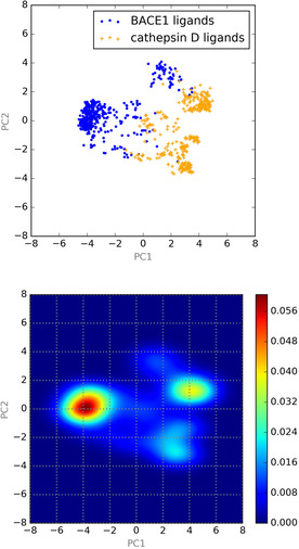
a(upper): Map of first (PC1) and second (PC2) principal components; b(lower): heatmap of the kernel density estimation the probability distribution.

3.3. Application of the Classifier/Decomposer for new Dataset

As seen in Figure 3a and Figure 3b, BACE1 and cathepsin D ligands were separately distributed in 2D space. Next, we wanted to understand how the mapping methodology functioned when applied to new datasets as subjects for the exploration of new ligand candidates. We used two datasets as input data to the GCNN model: one was a validation dataset for BACE1/ cathepsin D ligands, and the other was a dataset for natural compounds collected from the KNApSAcK database.7 We had no information about the binding properties of these natural compounds for BACE1/cathepsin D. Next, extracted feature vectors were decomposed using the same PCA model constructed for the training dataset as described above. The distributions of the components were visualized by scatterplots on the density map. As shown in Figure 4a, points for BACE1 and cathepsin D ligands accumulated in each chemical space. By contrast, Figure 4b shows that a majority of the points from natural compounds were distributed in the lower density space. Although some natural compound points were within the chemical space of cathepsin D ligands, few were within the space of BACE1 ligands.

Figure 4.

Map of principal components of known ligands overlaid on the probability density heatmap. a(upper): BACE1 (white) and cathepsin D (black) ligands; b(lower): 200 randomly selected natural compounds whose data are available in KNApSAcK database. The density map is the same as Figure 3b.

Therefore, the distributions of BACE1/cathepsin D ligands with high density differed significantly from those of the natural compounds. These results suggest the possibility that this process can be used to explore new candidate compounds that may have highly selective binding affinity to each protein. When data for new compounds are used as input data, and some are located near the distribution of a protein's ligand group in the probability density map, the probability is high that the new compounds belong to the ligand group of that protein. As discussed earlier, BACE1 is considered to be a good candidate treatment target for AD; therefore, we investigated the distribution of compounds in the KNApSAcK database on the probability density map generated from BACE1/cathepsin D (Figure 5) and counted the number of compounds located in the region where BACE1 ligands were concentrated (PC1 from −5 to −3 and PC2 from −0.5 to 1). As a result, 368 natural compounds were selected as potentially having highly selective binding affinity for BACE1. By contrast, 3,845 compounds were located in the chemical spaces where cathepsin D ligands exist at a higher density.

Figure 5.

Map of principal components of natural compounds. a (upper): Estimated probability density map of the distribution of the first and second principal components of 50,000 natural compounds; b(lower): Location of feature vectors from natural compounds after decomposition through PCA on the probability (right) density map showing the chemical space of the BACE1/cathepsin D ligand groups. Scatterplots in white show the location of natural compounds. The density map was generated from the training dataset for BACE1/cathepsin D ligand classification. The number of compounds located in the chemical spaces of BACE1, PC1 [−5, −3] and PC2 [−0.5, 1], was 368. For the chemical spaces of cathepsin D ligands, 3,583 compounds were in the region with PC1 [3, 5] and PC2 [1,2], and 262 were in the region with PC1 [2.5, 3.5] and PC2 [−3.5, 2.5]. (right). For both (a) and (b), a probability density map was generated from the training dataset for BACE1/cathepsin D ligands

4. Discussion

In the present study, we constructed a classification model to distinguish between ligands for a major target protein and those for an off‐target protein using a GCNN, selecting BACE1 and cathepsin D as example proteins. Feature vectors generated through the convolution/pooling processes were visualized in 2D maps after decomposition by PCA, and their probability density was calculated by kernel density estimation. This process could be expected to allow visualization of the localized distribution of both ligand groups, and may be useful for the evaluation of the ligands’ selectivity. In case of just using the GCNN model for classification, the output should indicate that the compounds are BACE1‐specific or cathepsin D specific. However, most compounds in the world must be none of them. That is why we suggested the approach to clarify chemical space of compounds feasible for evaluation in advance. We chose Binding DB as a good candidate dataset for use in the model construction and performance testing because it includes many types of molecular properties of various protein ligands. Some may wonder why we did not use the binding scores as objective variables and construct models that directly predicted the binding affinity to both BACE1 and cathepsin D. One problem we face when using an open‐source database such as Binding DB is that values relating to the binding affinity of ligands for proteins, e. g., inhibition and dissociation constants, are not consistent, and are difficult to compare directly. In such cases, it is not appropriate to use these values as objective variables to predict the binding properties by regression. Instead, we can consider categorizing these ligands in accordance with their binding affinity, and dealing with them as classification problems. That is why we set the classification processes described above instead of using regression.

The GCNN functioned very well for constructing the classification model to distinguish between ligands for BACE1 and those for cathepsin D. The classification performance was remarkably better than that of the other traditional classifiers, such as random forest and SVMs.

A scatter plot of principal components and a probability density map generated from the extracted feature vectors through the GCNN indicated that we successfully extracted the structural properties that clearly separated the distributions of BACE1 and cathepsin D ligands on the 2D map. We used only the first and second principal components for the mapping. To ensure that the two components are enough to explain The contribution to total variance from the first and second principal components, 55 %, was much higher than the 31 % from the first and second principal components of feature vectors in CF (radius=3, count vector without hash function). In addition, the dimension of the feature vectors generated from GCNN was apparently less (256) than that from CF (7,709), implying that feature extraction through a GCNN is efficient enough to represent significant variance of the compound groups. Ligands for cathepsin D had a broader distribution than those for BACE1. This broadening was in the direction of the second principal axis, which is orthogonal to the first principal axis. The first principal axis is derived from the variance explaining the structural difference between ligands related to their target proteins. Therefore, we consider that the broadening merely indicates the structural variety of reported cathepsin D ligands.

Using the classifier and decomposer constructed through the training process of the GCNN, we investigated the distribution of feature vectors from the validation dataset of BACE1/cathepsin D ligands and the dataset of natural compounds. The distributions of BACE1 and cathepsin D ligands were clearly reproduced for the validation dataset, indicating the rigor of the result obtained during the training process. However, the distribution obtained from the dataset of natural compounds was in a significantly different space from that of BACE1/cathepsin D ligands. Based on the results, we were able to implement a comprehensive exploration of candidates for BACE1 or cathepsin D ligands with higher selectivity. To do the exploration, we extracted 368 natural compounds located in the chemical space of BACE1 ligands in the principal component map.

To ensure that these compounds are considered candidates of specific ligands, we investigated the chemical space of 268 non‐specific ligands, with high affinity to both BACE1 and cathepsin D (Figure 6). Such compounds also had the distribution clearly different from specific ligands. Compounds on the chemical space of BACE1 ligands were used as input data for the classifier, and extracted the logit values of the output channel. Compounds with higher values for the output channel of BACE1 ligands and lower values for cathepsin D ligands were considered to have potential binding affinity for BACE1. As examples, the 10 compounds with the highest logit values in the channel for BACE1 ligands were extracted (data in the area highlighted in red in Figure 7). The chemical structures of these compounds are shown in Figure 8.

Figure 6.

Map of principal components of non‐specific ligands, with high binding affinity to both BACE1 and cathepsin D, overlaid on the probability density heatmap. The density map is the same as Figure 3b.

Figure 7.

Scatter plot of the output values from GCNN before applying softmax function for 195 natural compounds, which are located on a chemical space of BACE1 ligands in probability density map. Compounds existing in the region highlighted with red would be considered good candidates for BACE1 ligands.

Figure 8.

Chemical structures of compounds extracted from the region highlighted in red in Figure 6. In accordance with their skeletal structures, these can be divided into four groups, from (a) to (d). Extracted compounds are identified by C_ID in KNApSAcK database.

In these 10 compounds, 9 compounds are purified from plantae (Menispermaceae, Apocynaceae and Amaryllidaceae). One common feature of these compounds is that they are 5‐ or 6‐membered heterocyclic compounds conjugated to an aromatic ring. In addition, these compounds can be divided into four groups based on their skeletal structures, implying that such structural features may be crucial for selective binding of compounds to BACE1. It is also possible that these compounds might merely belong to a tail of the distribution of natural compounds that coincidently overlaps the chemical space of BACE1 ligands. Even in this case, we can at least dramatically narrow down candidate ligands using this methodology.

In this study, we selected a dataset of natural compounds as a target for comprehensive exploration. The advantages of using natural products as targets of exploration have been pointed out:11 development of drugs derived from natural compounds is beneficial because these are easily obtainable compared with synthetic compounds, and drugs derived from natural compounds are considered to be biodegradable and to pose less risk of unpredictable residues in the human body and the environment. Although there are huge varieties of natural products because of the variety of species of plants, marine species, sponges, mushrooms, lichen, and animals, only a minority of these natural products have been investigated as candidates for new drugs. One limitation has been the difficulty in isolating natural compounds from living systems, but high‐resolution techniques of isolation and purification have been advancing. Moreover, there are currently many libraries available that store data on natural compounds, including SMILES information. Therefore, a convenient screening method would be beneficial to allow evaluation of the potential of these compounds as drugs. The methodology we suggested does not require excess time and calculation, implying the possibility of using it for rapid screening.

5. Conclusions

We suggested a new approach using a GCNN for the comprehensive exploration of compounds having highly selective binding affinity for proteins of interest. To evaluate the effectiveness of this approach, we successfully constructed a GCNN classification model and extracted structural features relating to the differences between ligands for BACE1 and those for cathepsin D. The probability density of the extracted features decomposed to principal components differed significantly between BACE1/cathepsin D ligands and natural compounds on a 2D map. This approach is considered beneficial for two main reasons: 1) it does not need a dataset of true negatives, which is difficult to collect, and 2) it has lower calculation costs compared with other methodologies, such as quantum chemistry‐based approaches to molecular dynamics simulation. Moreover, using natural compounds as targets of exploration is beneficial for many reasons. Application of the methodology established in this study could be expected to accelerate the exploration of new candidates for highly selective drug compounds.

Conflict of Interest

None declared.

Y. Miyazaki, N. Ono, M. Huang, M. Altaf-Ul-Amin, S. Kanaya, Mol. Inf. 2020, 39, 1900095.

References

- 1. Steele L. S., Can. Fam. Physician. 1999, 45, 917–9. [PMC free article] [PubMed] [Google Scholar]
- 2. Yan R., Lancet Neurol. 2014, 13, 319–29. [DOI] [PMC free article] [PubMed] [Google Scholar]
- 3. Zuhl A. M., Nat. Commun. 2016, 7, 13042. [DOI] [PMC free article] [PubMed] [Google Scholar]
- 4. Liu K., arXive preprint 2018, 1803.06236. [Google Scholar]
- 5. Eguchi R., BMC Bioinf. 2019, [Google Scholar]
- 6. Torng W., bioRxiv preprint 2018, 10.1101/473074v1. [Google Scholar]
- 7. Afendi F. M., Plant Cell Physiol. 2012, 53, e11-12. [DOI] [PubMed] [Google Scholar]
- 8. Shortridge M. D., J. Comb. Chem. 2018, 10, 948–58. [DOI] [PMC free article] [PubMed] [Google Scholar]
- 9. Glorot X., PMLR 2011, 15, 315–23. [Google Scholar]
- 10. Kingma D. P., arXiv preprint 2014, 1412.6980. [Google Scholar]
- 11.T. Engel, Applied Chemoinformatics: Achievements and Future Opportunities, First Edition. Wiley-VCH Verlag GmbH & Co. KGaA. 2018, 165–167.