Harmonization of Infant Cortical Thickness Using Surface-to-Surface Cycle-Consistent Adversarial Networks

Abstract

Increasing multi-site infant neuroimaging datasets are facilitating the research on understanding early brain development with larger sample size and bigger statistical power. However, a joint analysis of cortical properties (e.g., cortical thickness) is unavoidably facing the problem of non-biological variance introduced by differences in MRI scanners. To address this issue, in this paper, we propose cycle-consistent adversarial networks based on spherical cortical surface to harmonize cortical thickness maps between different scanners. We combine the spherical U-Net and CycleGAN to construct a surface-to-surface CycleGAN (S2SGAN). Specifically, we model the harmonization from scanner X to scanner Y as a surface-to-surface translation task. The first goal of harmonization is to learn a mapping G_X : X → Y such that the distribution of surface thickness maps from G_X(X) is indistinguishable from Y. Since this mapping is highly under-constrained, with the second goal of harmonization to preserve individual differences, we utilize the inverse mapping G_Y : Y → X and the cycle consistency loss to enforce G_Y (G_X(X)) ≈ X (and vice versa). Furthermore, we incorporate the correlation coefficient loss to guarantee the structure consistency between the original and the generated surface thickness maps. Quantitative evaluation on both synthesized and real infant cortical data demonstrates the superior ability of our method in removing unwanted scanner effects and preserving individual differences simultaneously, compared to the state-of-the-art methods.

1. Introduction

In recent years, large-scale multi-site infant neuroimaging datasets are increasingly facilitating the research on understanding early brain development with larger sample size and bigger statistical power [3,7]. However, directly combining neuroimaging data across scanners will unavoidably introduce the non-biological variance to the data, typically due to differences in imaging acquisition protocol (e.g., field of view, coil channels, gradient directions, etc.) and hardware (e.g., manufacturer, magnetic field strengths, etc.). Such unwanted sources of bias and variability are referred as “site effects” in [1] that are non-biological in nature and associated with different scanning parameters. Herein, we also use different sites to represent different scanners. In previous studies, the site effects have been long understood to hinder the accurate detection of imaging features [2] and preclude joint analysis of multi-site data [9]. Therefore, harmonizing neuroimaging data to both remove site effects and preserve biological associations is imperative for joint analysis of the multi-site data.

Several harmonization techniques have been developed for adult diffusion MRI [4,8]. However, there are very few published methods for harmonizing brain morphological properties from structural MRI, e.g., cortical thickness, which are highly associated with brain development and disorders. Fortin et al. [1] proposed a statistical data pooling tool that uses Combat (a batch-effect correction tool used in genomics) for adult cortical thickness harmonization. Combat estimates a linear model with additive and multiplicative site-effect coefficient at each cortical region, thus accounting for site differences. However, this method has several limitations. First, a linear model at the region level might not be able to account for the complex mapping between multi-site data. Second, their optimization procedure assumes that the site-effect parameters follow a particular parametric prior distribution (Gaussian and Inverse-gamma), which might not hold well in many scenarios of cortical property harmonization. Third, as a statistical tool, the major drawback of Combat is the weak generalization ability, because Combat processes all data at one time and treat them equally, making it sensitive to outliers. Forth, Combat is designed for harmonizing two sites into one intermediate site, which is not applicable for mapping one less reliable site (with low-quality data) to another more reliable site (with high-quality data).

While not developed explicitly for harmonization, a number of recently developed deep learning techniques [11,12] could potentially be adapted to address these issues. First, the spherical U-Net architecture [11] provides an effective Direct Neighbor (DiNe) filter to extend conventional convolutional neural network (CNN) to the cortical surface with an inherent spherical topology. It was originally designed for cortical surface parcellation [10] and achieves state-of-the-art performance, which could be used as a generator for site-to-site cortical surface property map translation. Second, since most neuroimaging studies do not have paired data across sites, the popular image generation technique CycleGAN [12] could be leveraged for the unpaired surface translation. Therefore, we propose to extend the conventional CycleGAN to cortical surface data based on spherical U-Net termed S2SGAN. Specifically, we model harmonization from site X to site Y as a surface-to-surface translation task. A preliminary goal of harmonization is to learn a mapping G_X : X → Y such that the distribution of G_X(X) is indistinguishable from the distribution of Y. Since this mapping is highly under-constrained, with the second goal of harmonization to preserve biological variance, we utilize the inverse mapping G_Y : Y → X and the cycle consistency loss to enforce G_Y (G_X(X)) ≈ X (and vice versa). Furthermore, we incorporate the correlation coefficient loss to guarantee the structure consistency between the original surface thickness maps and the generated maps.

2. Method

2.1. Loss Design

As shown in Fig. 1(a), suppose we have two cortical surface datasets obtained from two sites, site X and site Y. Our goal is to learn the cross-site mapping functions of cortical surface property (e.g., cortical thickness) maps G_X and G_Y for X → Y and Y → X mapping, respectively. In addition, discriminator D_X is used to distinguish real and generated site X surface maps, and discriminator D_Y is similarly for site Y. All the mapping and discrimination functions can be approximated by spherical neural networks. The objective of optimizing the whole model includes three types of losses: (1) an adversarial loss for matching the distribution of generated surface maps to the distribution in the target site; (2) a cycle-consistency loss to prevent generators from producing surface maps that are irrelevant to the inputs; and (3) a correlation coefficient loss to constrain structure consistency between original and generated surface maps.

Fig. 1.

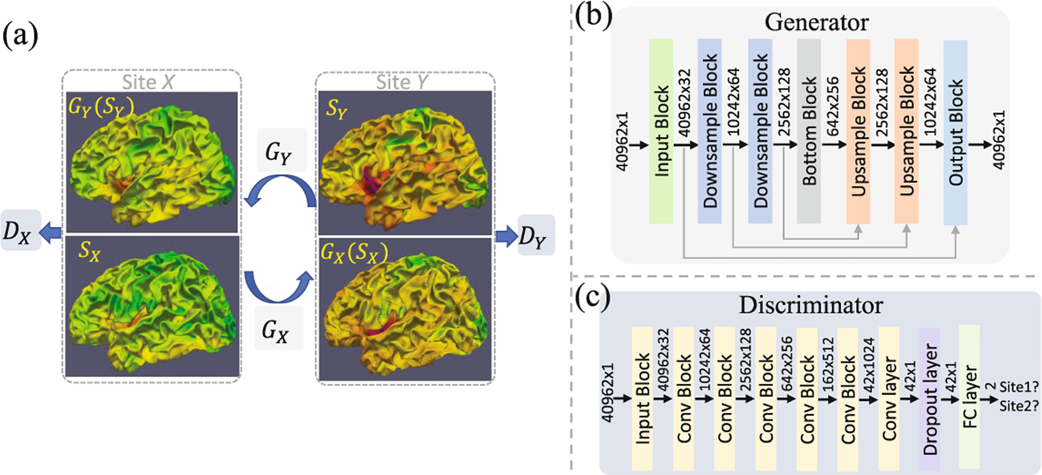
The framework of our proposed S2SGAN. (a) Two generators (G_X and G_Y) learn cross-site mappings of surface maps (herein, cortical thickness maps). Two discriminators (D_X and D_Y) distinguish generated surface maps and real surface maps. (b) In generators, each block contains repeated DiNeConv+BN+ReLU with input size and output size denoted before and after the block, and one more spherical pooling layer for each downsample block, one more spherical transposed convolution layer for upsample block to deal with the skip concatenated feature maps (grey arrows). (c) In discriminators, each block is DiNeConv+BN+ReLU+Pooling, except for the input block without pooling.

Adversarial Loss.

We apply adversarial loss to both mapping functions G_X : X → Y and G_Y : Y → X. For the mapping function G_X and its discriminator D_Y, the objective function is expressed as:

$${\mathcal{L}}_{GAN}\left(G_X,D_Y\right)=E_{x~p_{\mathit{\text{data}}}(X)}\left[{\left(1-D_Y\left(G_X(x)\right)\right)}^2\right]+E_{y~p_{\mathit{\text{data}}}(Y)}\left[D_Y{(y)}^2\right],$$

where x ~ p_data(X) and y ~ p_data(Y) denotes the data distribution of X and Y. G_X aims to generate surface maps G_X(x) close to the real target surface maps in site Y, while D_Y is to distinguish between generated surface maps and real surface maps of site Y. Therefore, the optimization of this minimax two-player game can be written as: ${\mathit{\text{min}}}_{G_X}{\mathit{\text{max}}}_{D_Y}{\mathcal{L}}_{GAN}\left(G_X,D_Y\right)$. A similar adversarial loss is also applied for G_Y and D_X.

Cycle-Consistency Loss.

To guarantee the generated surface maps are meaningful to the original surface maps, an additional cycle consistency loss [12] is defined as the difference between original and reconstructed surface maps:

$${\mathcal{L}}_{cyc}\left(G_X,G_Y\right)=E_{x~p_{\mathit{\text{data}}}(X)}\left[\Vert G_Y\left(G_X(x)\right)-x{\Vert }_1\right]+E_{y~p_{\mathit{\text{data}}}(Y)}\left[\Vert G_X\left(G_Y(y)\right)-y{\Vert }_1\right].$$

Correlation Coefficient Loss.

For cortical surface property maps, it is crucial to preserve local structural information in the mapping functions. To further reduce the ambiguity of indirect cycle-consistency loss between the original and generated surface maps, we adopt the correlation coefficient loss to enforce structure consistency between input and generated surface maps:

$${\mathcal{L}}_{cc}\left(G_X,G_Y\right)=-E_{x~p_{\mathit{\text{data}}}(X)}\left[\frac{\text{cov}\left(G_X(x),x\right)}{{\sigma }_{G_X(x)}{\sigma }_x}\right]-E_{y~p_{\mathit{\text{data}}}(Y)}\left[\frac{\text{cov}\left(G_Y(y),y\right)}{{\sigma }_{G_Y(y)}{\sigma }_y}\right],$$

where cov denotes the covariance, σ denotes the standard deviation.

(Optional) Paired Loss.

In our method, we don’t require any paried data from different sites for training, which are typically hard to acquire. However, if we have paired data, we can add an additional paired loss to directly constrain the vertex-wise similarity between the generated surface maps and the corresponding groundtruth surface maps:

$${\mathcal{L}}_{\mathit{\text{pair}}}\left(G_X,G_Y\right)=E_{x~p_{\mathit{\text{data}}}(X)}\left[\Vert G_X(x)-gt(x){\Vert }_1\right]+E_{y~p_{\mathit{\text{data}}}(Y)}\left[\Vert G_Y(y)-gt(y){\Vert }_1\right],$$

where gt(x), gt(y) represent the groundtruth of x and y in the paired dataset.

Full Objective.

Finally, the full objective of our model is written as: $\mathcal{L}\left(G_X,G_Y,D_X,D_Y\right)={\mathcal{L}}_{GAN}\left(G_X,D_Y\right)+{\mathcal{L}}_{GAN}\left(G_Y,D_X\right)+\alpha {\mathcal{L}}_{cyc}\left(G_X,G_Y\right)+\beta {\mathcal{L}}_{cc}\left(G_X,G_Y\right)+\lambda {\mathcal{L}}_{\mathit{\text{pair}}}\left(G_X,G_Y\right)$, where α, β, and λ control the relative importance of the loss terms. Note that the last loss term will be removed when having no paired data.

2.2. Network Architecture

We use the spherical U-Net [11] architecture as our generative network. Leveraging the spherical topology of cortical surfaces, the spherical U-Net first extends convolution, pooling, and upsampling operations to the spherical space using DiNe filter on regularly resampled spherical surfaces, and then constructs U-Net using corresponding spherical operations. We modified the spherical U-Net with half feature channels and 4 resolution steps, first 3 of which are concatenated with skip connections; see Fig. 1(b) for more detailed information. For the discriminator network, we extend a VGG style classification CNN to spherical surfaces. It consists of 7 DiNe convolution layers, 5 spherical pooling layers, a dropout layer with probability 0.2, and 1 fully connected layer, as shown in Fig. 1(c). Note all the DiNe convolution layers are followed by batch normalization (BN) and leaky rectified linear unit (ReLU) with negative slope of 0.2.

3. Experiments and Results

3.1. Validation on Synthetic Paired Surface Data

To better evaluate the performance of our method for harmonizing cortical thickness maps across sites, we synthesized a paired dataset to simulate cortical surfaces reconstructed from images scanned at different resolutions, which is a typical occurrence in harmonization task. Specifically, we used the BCP dataset [3] from one scanner, with 360 MRI scans from 183 infants and age from 0 to 2 years, named site X. Both T1w and T2w images were acquired at the resolution of 0.8 × 0.8 × 0.8 mm³. We resampled all T1w and T2w images in site X to 1 × 1 × mm³ to form another dataset, site Y. All MR images were processed using an infant-dedicated computational pipeline [6]. All cortical surfaces were mapped onto the spherical space, nonlinearly aligned, and further resampled.

In our experiment, for S2SGAN model without paired data, we set α as 15, β as 1, and λ as 0; for S2SGAN model with paired data, we set α as 15, β as 1, and λ as 100. We trained both models using Adam optimizer to alternately update G and D with an initial learning rate 0.0001 for the first 20 epochs and linearly-reduced rate to 0 for the next 180 epochs. We used 70% of the data as the training set and remaining 30% as the testing set using stratified sampling. We used two well accepted metrics of mean absolute error (MAE) and peak signal-noise ratio (PSNR) for quantitatively evaluating the results.

We compare the harmonization results from site Y with low quality data to site X with high quality data. On average, our S2SGAN achieves MAE 0.0928 ± 0.0109 mm, PSNR 31.48 ± 1.116 (the standard deviation is between scans). The S2SGAN (paired) model achieves MAE 0.082 ± 0.0178 mm and PSNR 33.09 ± 1.727, which represents the best that a S2SGAN can achieve. For comparison, the Combat [1] results were obtained by using the official code with age and gender as biological covariates, achieving MAE 0.124 ± 0.0137 mm and PSNR 29.00 ± 1.019. In all, our S2SGAN achieves better performance than Combat in both MAE and PSNR and also produces closer results to S2SGAN (paired). Figure 2 shows the harmonization results of different methods on a testing subject.

Fig. 2.

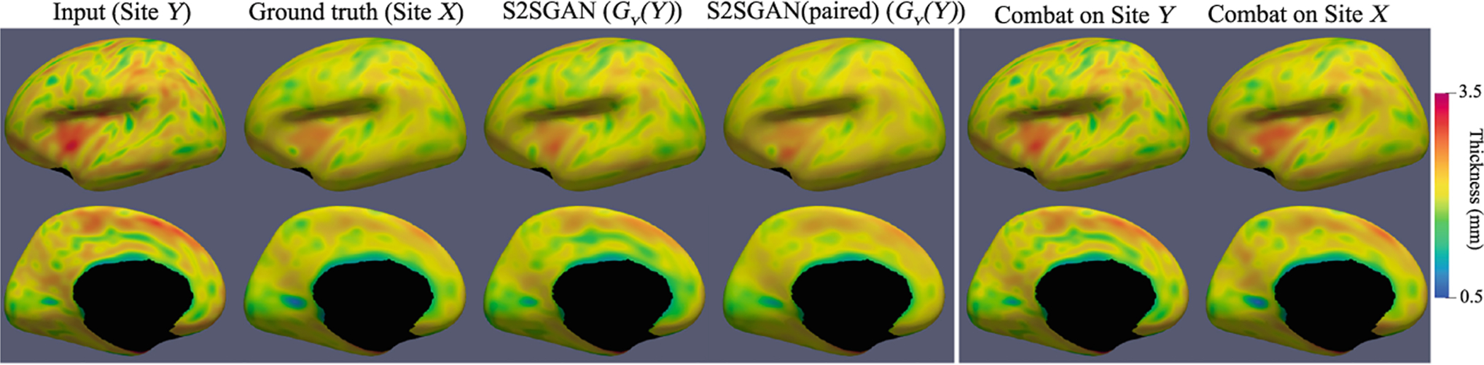
Comparison of harmonization results using different methods on a testing subject. The first four columns show the S2SGAN model results. The last two columns show the Combat results. Note that Combat harmonizes two sites into one intermediate site, thus should generate two identical surfaces in the last two columns.

3.2. Validation on Real Unpaired Surface Data

To demonstrate the practical ability of our method in harmonizing cortical thickness across sites, we employed two real longitudinal infant datasets with matched demographics. Site X is the same dataset in Sect. 3.1. Site Y has 251 longitudinal scans from 50 infants, acquired at the resolution of 1 × 1 × 1 mm³, from a different scanner. We trained our S2SGAN model using the same experimental configuration as in Sect. 3.1.

Validation on Removing Site Effects.

For unpaired data, we use the same evaluation method in [5] to perform ROI-based analysis to estimate if the site effects are removed. With matched demographics, we aim to achieve the same average ROI thickness values as the target site after harmonization. In Fig. 3, we show the 36 mean ROI thickness values of site X, site Y, and harmonized site Y. We observed that statistical differences of ROI thickness are significant prior to harmonization and are successfully removed after harmonization. Same as in [1], we also performed unsupervised dimension reduction on all vertex-wise thickness data: site X + site Y + harmonized Y, using PCA. The data projected into the first two principal components are presented in Fig. 4. Figure 5 shows the boxplots of vertex-wise thickness for stratified sampled 100 subjects from site X, site Y and harmonized Y, sorted by age. We note that our method not only achieves similar distribution as the target site, but also well preserves the individual differences.

Fig. 3.

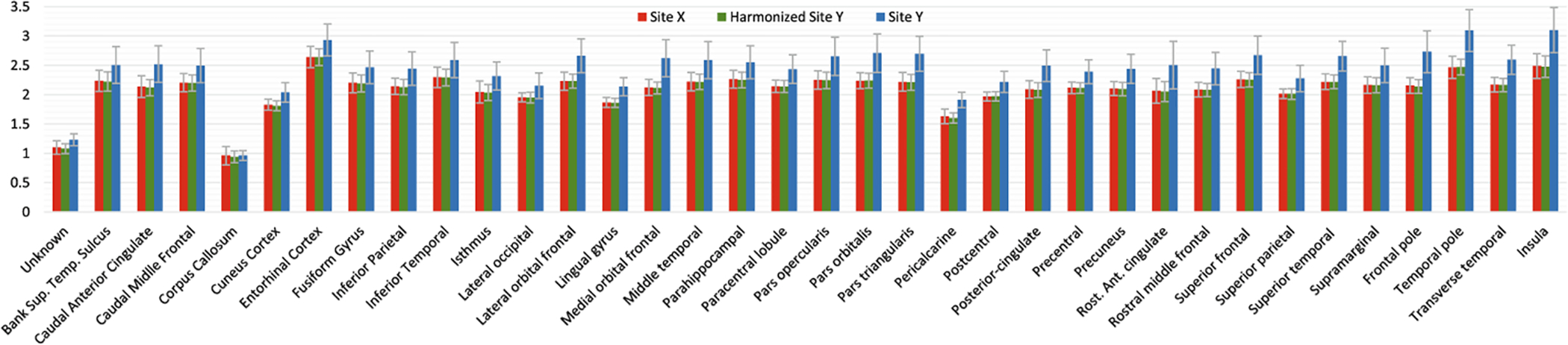
Comparison of cortical thickness value across sites for each ROI.

Fig. 4.

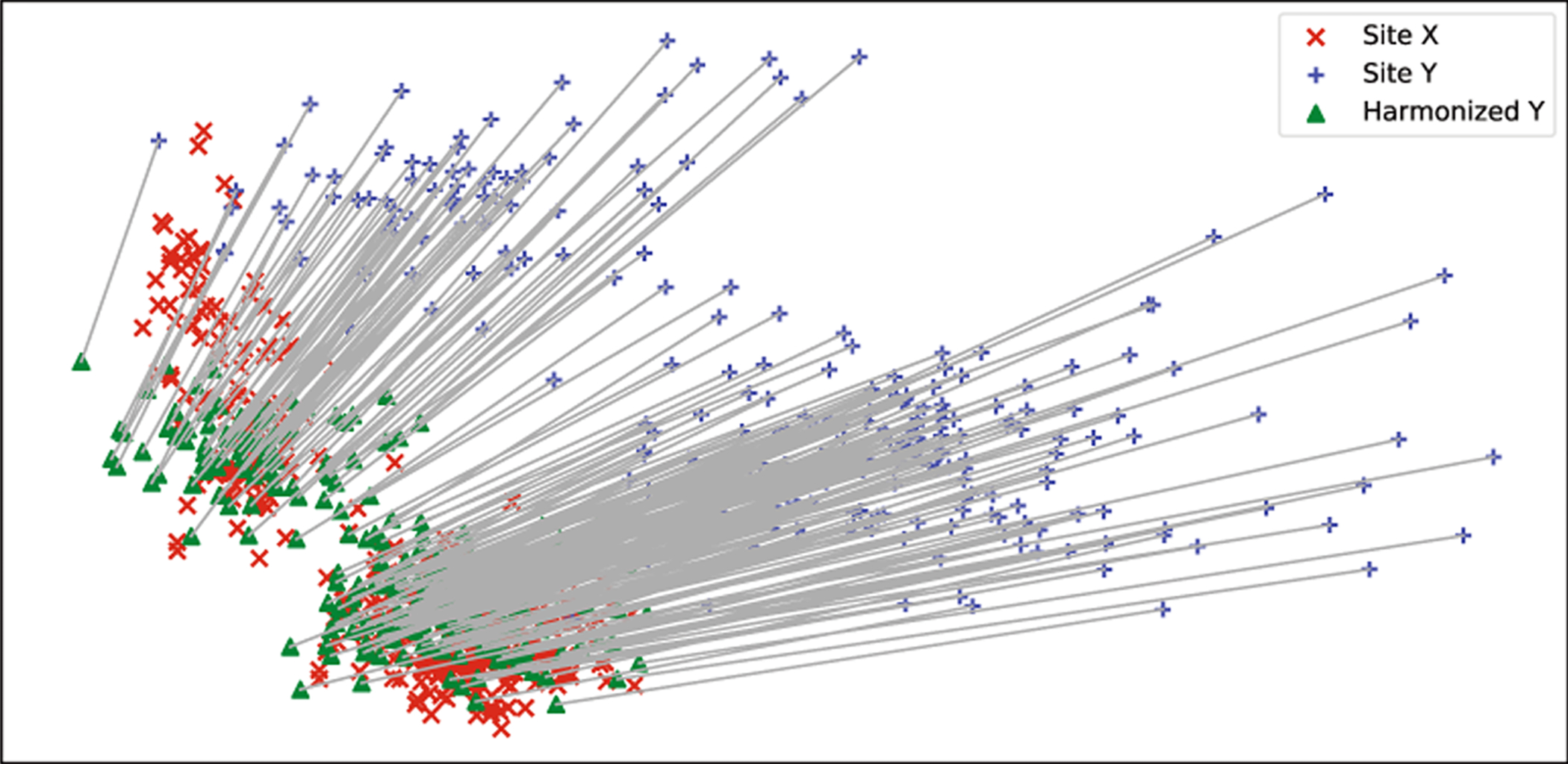
Dimension reduction results of site X + site Y + harmonized site Y using PCA. The x-axis is the first principal component and y-axis is the second principal component. The grey lines represent the correspondences of the same scans before and after harmonization.

Fig. 5.

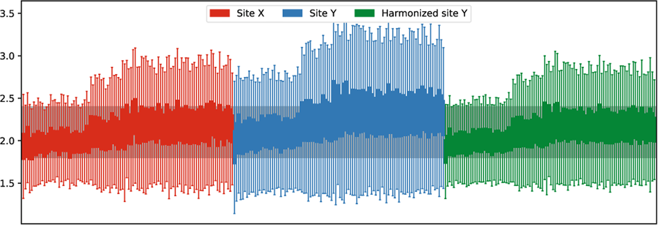
Boxplots of vertex-wise thickness for different sites. Each boxplot represents a scan. Stratified sampled 100 scans are presented for each site and are sorted by age within the site.

Validation on Preserving Group Differences.

Same as in [5], we adopted Cohen’s d for evaluating age group differences preservation. Cohen’s d is defined as the group differences: $d_{ij}=\frac{1}{N_r}\sum _r\left|\left(M_{ir}-M_{jr}\right)/\sqrt{\frac{\left(n_i-1\right)s_{ir}^2+\left(n_j-1\right)s_{jr}^2}{n_i+n_j-2}}\right|$, where i and j represent two groups, r represents each ROI feature, N_r is the number of ROIs, M is the mean cortical thickness, s is the standard deviation and n is the number of subjects in the group. Cohen’s d is thus free of data value size and generally ranges from 0.1 to 2.0, proportional to the effect sizes between groups. We divided all the data into 6 groups separated by 45, 135, 225, 315, and 450 days of age and compute Cohen’s d for each two of them. The Δd is then computed as the mean absolute deviation of Cohen’s d before and after harmonization: $\Delta d=\frac{1}{N_g\left(N_g-1\right)}\sum _{i=1}^{N_g}\sum _{j\ne i}^{N_g}|d_{ij}^{\mathit{\text{before}}}-d_{ij}^{\mathit{\text{after}}}|$, where N_g is the number of groups and $d_{ij}^{\mathit{\text{before}}}$, $d_{ij}^{\mathit{\text{after}}}$ represent the Cohen’s d before and after harmonization, respectively. Thus a smaller Δd generally represents a better difference preservation. For comparison, we adopted Combat using the official code with age as biological covariate. On average, our S2SGAN achieves Δd 0.0683 ± 0.0520 and Combat achieves Δd 0.2069 ± 0.1467 (the standard deviation is between group pairs). With a smaller Δd, we can conclude that our method better preserves the group differences in brain development.

Validation on Preserving Individual Differences.

Instead of using median values in [4], we use ROI feature values to compute Euclidean distances between any two scans, thus forming a distance matrix, denoted as $E_{ij}^{n\times n}={\Vert F_i-F_j\Vert }_2$, where n is the number of scans, and F is the feature vector. The goal is to estimate how the distances are preserved relatively to each other before and after harmonization. Therefore, we compute the correlation Cor of the two distance matrices before and after harmonization. We also adopted Combat with age and gender as biological covariates for comparison. Our S2SGAN achieves Cor 0.9766, and Combat achieves Cor 0.9606. With a higher Cor, we can conclude that our method better preserves the individual differences. Figure 6 shows two age-matched subjects’ harmonization results. We can see that the differences both between subjects and ages are well preserved.

Fig. 6.

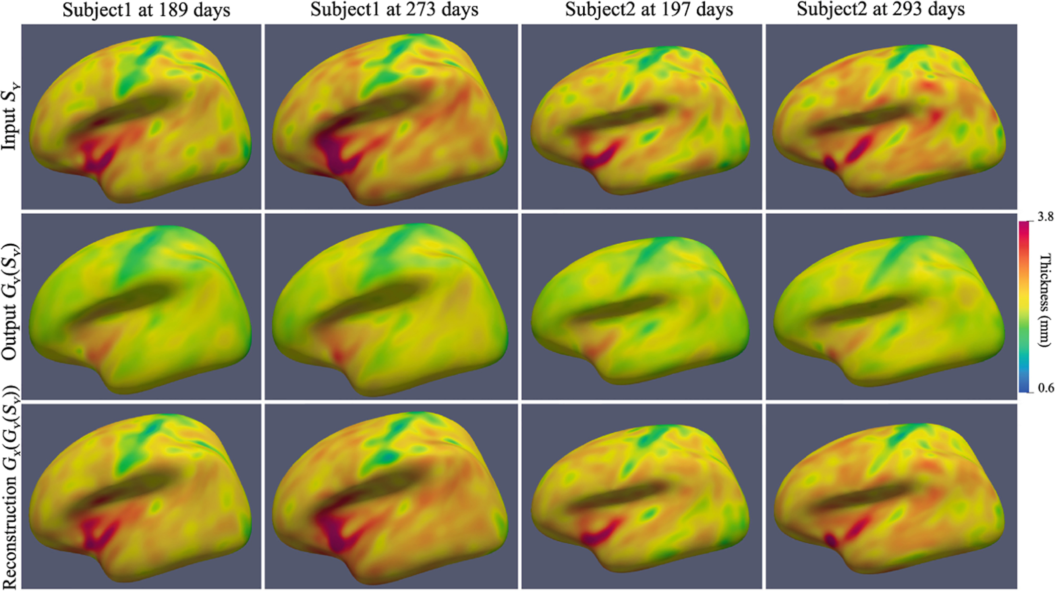
Visualization of harmonization results on two age-matched testing subjects.

4. Conclusion

In this paper, we propose a novel cortical thickness harmonization method, based on spherical U-Net to learn the inherent complex mapping from one site to another site in a CycleGAN manner. Our proposed method, S2SGAN, has been validated on both synthetic paired data and real unpaired data of infant brain MRI. Both visual and quantitative results demonstrate its superior capability to reduce inter-site variance, while preserving individual variance simultaneously.

References

- 1.Fortin JP, et al. : Harmonization of cortical thickness measurements across scanners and sites. Neuroimage 167, 104–120 (2018) [DOI] [PMC free article] [PubMed] [Google Scholar]
- 2.Han X, et al. : Reliability of mri-derived measurements of human cerebral cortical thickness: the effects of field strength, scanner upgrade and manufacturer. Neuroimage 32(1), 180–194 (2006) [DOI] [PubMed] [Google Scholar]
- 3.Howell BR, et al. : The UNC/UMN baby connectome project (BCP): an overview of the study design and protocol development. NeuroImage 185, 891–905 (2019) [DOI] [PMC free article] [PubMed] [Google Scholar]
- 4.Huynh KM, et al. : Multi-site harmonization of diffusion mri data via method of moments. IEEE Trans. Med. Imaging 38, 1599–1609 (2019) [DOI] [PMC free article] [PubMed] [Google Scholar]
- 5.Karayumak SC, et al. : Retrospective harmonization of multi-site diffusion MRI data acquired with different acquisition parameters. Neuroimage 184, 180–200 (2019) [DOI] [PMC free article] [PubMed] [Google Scholar]
- 6.Li G, et al. : Construction of 4D high-definition cortical surface atlases of infants: methods and applications. Med. Image Anal 25(1), 22–36 (2015) [DOI] [PMC free article] [PubMed] [Google Scholar]
- 7.Li G, et al. : Computational neuroanatomy of baby brains: a review. Neuroimage 185, 906–925 (2019) [DOI] [PMC free article] [PubMed] [Google Scholar]
- 8.Mirzaalian H, et al. : Harmonizing diffusion MRI data across multiple sites and scanners. In: MICCAI, pp. 12–19 (2015) [DOI] [PMC free article] [PubMed] [Google Scholar]
- 9.Takao H, et al. : Effect of scanner in longitudinal studies of brain volume changes. J. Magn. Reson. Imaging 34(2), 438–444 (2011) [DOI] [PubMed] [Google Scholar]
- 10.Zhao F, et al. : Spherical U-Net for infant cortical surface parcellation. In: ISBI, pp. 1882–1886 (2019) [DOI] [PMC free article] [PubMed] [Google Scholar]
- 11.Zhao F, et al. : Spherical U-Net on cortical surfaces: methods and applications. In: IPMI, pp. 855–866 (2019) [DOI] [PMC free article] [PubMed] [Google Scholar]
- 12.Zhu JY, et al. : Unpaired image-to-image translation using cycle-consistent adversarial networks. In: ICCV, pp. 2223–2232 (2017) [Google Scholar]