Single-cell reconstruction of emerging population activity in an entire developing circuit

Summary

Animal survival requires a functioning nervous system to develop during embryogenesis. Newborn neurons must assemble into circuits producing activity patterns capable of instructing behaviors. Elucidating how this process is coordinated requires new methods that follow maturation and activity of all cells across a developing circuit.

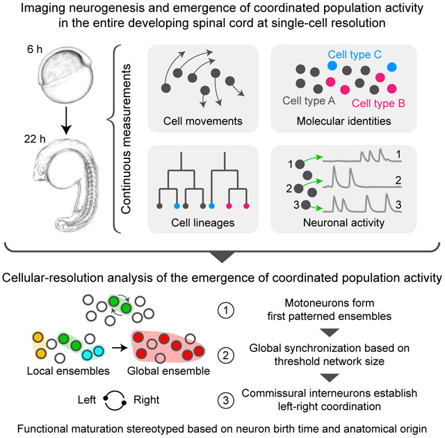
We present an imaging method for comprehensively tracking neuron lineages, movements, molecular identities, and activity in the entire developing zebrafish spinal cord, from neurogenesis until the emergence of patterned activity instructing the earliest spontaneous motor behavior.

We found that motoneurons are active first and form local patterned ensembles with neighboring neurons. These ensembles merge, synchronize globally after reaching a threshold size, and finally recruit commissural interneurons to orchestrate the left-right alternating patterns important for locomotion in vertebrates. Individual neurons undergo functional maturation stereotypically based on their birth time and anatomical origin. Our study provides a general strategy for reconstructing how functioning circuits emerge during embryogenesis.

Graphical Abstract

In brief

Wan et al. reconstruct neurogenesis and the emergence of coordinated neuronal activity at the single-cell level in the zebrafish spinal cord by tracking neuron lineages, movements, molecular identities, and activity in the entire developing circuit. They find that functional maturation of neurons is stereotyped, based on birth time and anatomical origin, and that early motoneuron activity leads ensembles that synchronize globally, based on network size.

Introduction

For a functioning animal to develop during embryogenesis, circuits need to assemble from individual neurons and form functional networks capable of orchestrating behaviors crucial for survival. The assembly of these neural circuits requires neurons to acquire their functional identities, form connections with each other, and generate patterned neural activity as a network to perform computations and instruct behaviors. To succeed in this task, the developmental programs of the neurons that form a circuit must be coordinated in space and time, from the moment they are born until network activity is reliably produced.

Population activity in developing circuits critically reflects the structural and functional organization of the emerging network and can itself influence the developmental process (Blankenship and Feller, 2010; Katz and Shatz, 1996; Kirkby et al., 2013; Moody and Bosma, 2005). Our understanding of circuit development has benefitted tremendously from in vivo and in vitro recordings of population activity in circuits related to sensory (Lippe, 1994; Meister et al., 1991; Torborg and Feller, 2005; Wiesel and Hubel, 1963), motor (Landmesser and O'Donovan, 1984; Wenner and O'Donovan, 2001) and cognitive functions (Cattani et al., 2007; Corlew et al., 2004; Garaschuk et al., 2000; Rubenstein and Rakic, 2013). However, it has not been possible so far to follow individual neurons throughout whole-circuit development, which precluded continuous measurements of circuit-wide activity at the single-cell level as well as the circuit-wide tracking of cell identities and developmental lineages. These fundamental limitations constrain our ability to (1) study the functional maturation of individual neurons and their role in the emergence of network activity, (2) dissect how the network state dynamically changes during development, and (3) elucidate how neurons collectively form entire circuits capable of producing patterned network activity. A comprehensive measurement of emerging population activity in an entire developing circuit at the single-neuron level would offer unprecedented access to these questions.

Here we developed and applied a light-sheet imaging assay and computational framework capable of systematically reconstructing, at the single-cell level, the emergence of coordinated population activity throughout an entire circuit from neurogenesis to the onset of behavior. Using the capabilities provided by our approach, we set out to investigate how the earliest functioning circuit, the motor circuit in the spinal cord, emerges during zebrafish embryogenesis.

In many vertebrates and invertebrates, motor activity occurs spontaneously during early embryonic development, without a need for external stimuli (Hamburger, 1963; Provine, 1972), and its emergence is a fundamental first step reflecting de novo circuit assembly in the nervous system (Blankenship and Feller, 2010; Borodinsky et al., 2004; Hanson and Landmesser, 2004; Hanson et al., 2008). The zebrafish offers several advantages for studying motor circuit development (Fetcho et al., 2008; Fetcho and Liu, 1998). Embryos develop rapidly and show transient, spontaneous motor behaviors by the end of the first day of embryogenesis in the form of slow tail contractions alternating between the left and right side. Spontaneous motor network activity is mediated from within the spinal cord by motoneurons (MNs) electrically coupled to interneurons (INs) on the same side of the body (Saint-Amant and Drapeau, 2000, 2001; Warp et al., 2012), and one IN type was identified in rostral segments as pacemaker INs generating rhythmic activity patterns (Tong and McDearmid, 2012). Intermittent calcium recordings in subsets of neurons in the embryonic spinal cord furthermore suggested correlated activity to be associated with strengthening of ipsilateral connections (Warp et al., 2012). In addition, developmental studies uncovered mechanisms underlying cell fate determination (Jessell, 2000; Lewis and Eisen, 2003), axonal pathfinding (Eisen et al., 1986; Kuwada et al., 1990; Myers et al., 1986; Pike et al., 1992), and cell subtype specification (Lewis and Eisen, 2004; Moreno and Ribera, 2010). The relative simplicity of the early spinal cord has provided us with an opportunity to work towards a systems-level understanding of motor circuit development and connecting mechanisms underlying neural development to the emergence of network function at the whole-circuit level.

We simultaneously measured cell movements, lineages, and calcium dynamics of all neurons across multiple segments of the embryonic spinal cord. Thereby, we characterized circuit development and activity with single-cell resolution and continuous temporal coverage throughout development, while annotating individual cells and cell types using anatomical and cell type-specific markers. Using our computational methods, we then extracted and analyzed the corresponding single-neuron activity traces, and modeled the emergence of patterned activity and changes in activity patterns in the neuronal network throughout development. We integrated these analyses with functional perturbation experiments to dissect the underlying network properties and roles of different cell types in circuit maturation.

Our systematic reconstruction of the emergence of function in the spinal circuit reveals how patterned activity develops in the early motor circuit. First, MNs with stereotypic soma locations emerge as the earliest active neurons and form local ensembles by recruiting neighboring neurons that inherit their activity signatures. Next, these local patterned ensembles coalesce and grow beyond a threshold network size required for global network synchronization. Finally, dorsal commissural INs are recruited to the emerging network and establish left-right alternating oscillations, which concludes the maturation of the activity pattern underlying the earliest spontaneous motor behavior.

We furthermore analyzed the relationships between neuronal cell lineages, movements and activity patterns, and discovered multiple links between neurogenesis and the emergence of neuronal activity and circuit function. By constructing a dynamic atlas that integrates our data of the anatomical, developmental and functional properties of all active neurons in the early spinal circuit, we reveal how a functioning circuit emerges during embryogenesis and establish a general paradigm for dissecting population activity throughout circuit development.

Results

Long-term imaging of development and functional maturation of the embryonic spinal cord with single-cell resolution

To understand the dynamic process of building a functional motor circuit during zebrafish embryogenesis, we developed an experimental protocol for imaging entire embryos throughout neurogenesis and capturing the developmental origins of neurons, which is seamlessly followed by longitudinal functional imaging of population-wide neuronal dynamics in the spinal cord at the single-cell level until patterned activity emerges (Fig. 1A-C). This approach captures long-term dynamics of activity in the developing spinal circuit while simultaneously identifying cell types and tracking cell identities and lineages from the neural plate to the embryonic spinal cord.

Figure 1 ∣. Imaging and data analysis framework for reconstructing development and functional maturation of the embryonic spinal cord at the single-cell level.

(A) Experimental paradigm and computational workflow for combined whole-embryo developmental imaging and longitudinal functional imaging of developing zebrafish spinal cord.

(B) Lateral-view snapshots of developmental imaging data. Blue: ubiquitous reporter, yellow: MNs and ventral INs.

(C) Dorsal-view snapshots of functional imaging data of embryonic spinal cord. Grey: GCaMP6f baseline.

(D) Dorsal- and lateral-view snapshots of mnx1 expression pattern at 22 hpf. Grey: GCaMP6f baseline.

(E) Curated cell tracks of active neurons in spinal cord over 4.5 hours of functional imaging. Time color-coded red to blue.

(F) Example traces of long-term activity in single neurons.

(G) Single-neuron activity traces of all active neurons in spinal circuit within field-of-view at 17.5, 19.5, 21 hpf. Neuron order is preserved across time windows and examples from (F) are highlighted.

(H) Cell type identification of active neurons. Top: locations of active neurons on left (green) and right (magenta) sides of spinal cord, overlaid with mnx1 channel (gray). Bottom: enlarged view of boxed region (left: cross-section, right: side view). Arrows indicate soma locations of mnx− active neurons on dorsal side.

(I) Characterization of mnx+ and mnx− cell morphologies. Top: elavl3 (blue) and mnx1 (green) expression at 24 hpf. Bottom: labeling of active mnx− neuron by electroporation (contralateral and ascending projection to hindbrain, imaged at 2 dpf). Magenta channel gamma-corrected to visualize thin processes. Cross-section (left) and side view (right).

Hours pf (or hpf), hours post fertilization; A, anterior; P, posterior; L, left; R, right; D, dorsal; V, ventral.

Scale bars: 50 μm (B, left; H, top), 20 μm (B, right; C; D; H, bottom; I).

See Movies S1, S2A, S3, S4; Fig. S1.

To block spontaneous muscle contractions throughout neural development while keeping patterned neuronal activity intact, we injected zebrafish embryos with a custom-designed, membrane-tethered alpha-bungarotoxin mRNA at the one-cell stage (Fig. S1A,B; Methods). We then mounted these embryos, which expressed a ubiquitous nuclear marker, a pan-neuronal nuclear-targeted calcium indicator, and a cell type-specific marker, at the shield stage (6 hours post fertilization, hpf). To follow embryonic development, we first used simultaneous multi-view light-sheet microscopy (SiMView) (Tomer et al., 2012) to image the ubiquitous and cell type-specific markers across the entire embryo from four angles in 90-second intervals until the 20-somite stage (17.5 hpf) when spontaneous activity first emerges in the nervous system (Movie S1A; Fig. 1B). We then seamlessly transitioned to longitudinal functional imaging from 17.5 to 22 hpf of all post-mitotic neurons across 9-10 segments of the spinal cord at 4 Hz, using hs-SiMView light-sheet microscopy (Lemon et al., 2015). We also acquired images of cell-type specific markers during functional imaging, while the nuclear-localized calcium indicator served as a readout for single-cell neuronal activity (Movie S2A; Fig. 1C,D).

We used the whole-embryo developmental imaging data for cell tracking and lineage reconstructions of all neurons identified from the functional imaging data (Movie S1A), as well as for creating a multi-specimen database integrating development, function, anatomy, and molecular profiles of neurons in circuit development. In addition, we used the functional imaging data to reconstruct the process of emergence of population neuronal activity. To this end, we first identified the spatial locations of all neurons from the image data of the pan-neuronally expressed calcium indicator, which covers all cells in the spinal cord expressing HuC/HuD (Movie S3A). We then developed a semi-automated computational method for accurate reconstruction of the movements of all cells over the 60,000 time points each recording comprises (Movie S3B; Figs. 1E, S1C; Methods). We furthermore annotated cell types using the cell type-specific markers employed during live imaging and by immunolabeling at the end of time-lapse acquisition. Finally, we spatially registered the developmental, functional and cell-type image data at the single-cell level in order to jointly analyze neuron lineages, molecular information and functional properties.

Using the calcium imaging data, we measured single-cell activity across several hundred neurons over 4.5 hours of development, from the onset of sporadic single-neuron activity to emergence of circuit function (Fig. 1F). We observed that the globally coordinated circuit activity pattern forms within a short period of time: spontaneous single-neuron activity emerges at ~17.5 hpf; at ~19 hpf, several small groups of neurons exhibit patterned activity while activity of other neurons remains sporadic; by ~22 hpf all active neurons have formed a globally synchronized ensemble, with the left and right sides of the spinal cord showing the alternating pattern required for early motor behaviors (Fig. 1G). This coarse description at the population level is in agreement with previous studies (Saint-Amant and Drapeau, 2000, 2001; Warp et al., 2012) and with results we obtained using cytoplasmic-localized calcium indicators (Movie S3C). Interestingly, in non-immobilized fish, spontaneous muscle contractions occur before the onset of large-scale patterned activity in the nervous system; however, by 22 hpf neural activity and muscle activity are synchronized and motor events occur with comparable frequency and left-right alternation index in immobilized and non-immobilized embryos (Fig. S1B).

To identify cell types and investigate the role of individual cells in development, we integrated cell type-specific genetic markers in our imaging assay, which complement the pan-neuronal calcium indicator used for functional imaging. We used the line Tg(mnx1:TagRFP-T) (Jao et al., 2012) to label a sub-population of cells that includes MNs and ventral longitudinal descending INs (VeLDs) in the ventral spinal cord (Fig. 1D). When overlaying cell locations in this fluorescently labeled mnx+ population with those of active neurons (Movie S4A; Fig. 1H), we found a separate active mnx− population that is located more dorsally. To identify the cell types these mnx− neurons belong to, we used single-cell electroporation to selectively label active mnx− neurons. All labeled cells in the mnx− population that exhibited patterned activity were commissural neurons (Fig. 1I, n = 6), which send axons ventrally, across the midline and then predominantly ascendingly toward the hindbrain. Since commissural primary ascending (CoPA) INs were shown to be involved in sensory gating but not active in the spontaneous coiling circuit (Higashijima et al., 2004; Knogler and Drapeau, 2014), we hypothesize that this mnx− population consists of commissural secondary ascending (CoSA) INs. Some (two out of six) of the commissural neurons labeled by electroporation show bifurcating projection patterns with a secondary branch projecting descending axons at the larval stage. These neurons are likely commissural longitudinal ascending (CoLA) INs (Hale et al., 2001; Liao and Fetcho, 2008). The commissural morphology of these mnx− neurons is also apparent from our functional imaging data of pan-neuronal cytosolic GCaMP acquired together with the mnx1:TagRFP marker (Movie S4B; Fig. S1D). We furthermore found the population of active mnx− neurons to overlap substantially with glycinergic neurons labeled by a Tg(glyt2-hs:loxP-DsRed-loxP-ChR) line (Kimura et al., 2014), suggesting that these mnx− neurons have a glycinergic identity. Notably, cerebrospinal fluid-contacting Kolmer-Agduhr (KA) neurons also exhibit sporadic, spontaneous activity, as described previously (Hubbard et al., 2016; Sternberg et al., 2018); however, they do so relatively late in the functional development of the spinal cord and their activity is not synchronized or in phase with the patterned motor network (Fig. S1E-H).

Circuit-wide, longitudinal analysis of single-neuron activity reveals stereotyped maturation of coordinated population activity

Next, we set out to reconstruct the emergence of coordinated population activity from our population-wide data of single-neuron activity traces. To examine the intrinsic structure of the data and reveal the principles underlying long-timescale evolution of circuit dynamics in the zebrafish spinal cord, we developed a framework based on factor analysis. Factor analysis is a multivariate statistics approach that seeks to explain the variance in a set of jointly measured attributes as a combination of a small number of shared factors, plus a residual individual variability in each attribute (Fig. 2A). Factor analysis is useful for analyzing neural population activity, since neurons are often strongly influenced by a set of shared components (Wei et al., 2019; Yu et al., 2009a), and thus neurons with strong shared components can be grouped into patterned ensembles. Moreover, the inherent separation between activity that can be described by isolated single neuron variability and that described by shared variability is of particular interest, since it can serve as a metric for the synchronization level of population activity.

Figure 2 ∣. Circuit-wide, longitudinal analysis of single-neuron activity reveals stereotyped maturation of coordinated population activity.

(A) Illustration of factor analysis: high-dimensional population activity (activity of all active neurons) modeled by low-dimensional shared dynamical modes (activity of patterned ensembles) that contribute to individual neuron activity with different weights, plus individual residuals.

(B) Top: location of patterned ensembles in developing spinal cord over time. Colors indicate different ensembles. Bottom: dorsal-view map of ensembles at six time points (horizontal dashed lines: segmental boundaries, vertical dashed line: midline, filled/open circles: active/inactive neurons). Active neurons in same colored patch belong to same ensemble.

(C) Time-dependent fractions of active neurons (red) and non-factored neurons (black). Circles: raw data. Lines: sigmoidal fits. Phases of circuit maturation colored as in (B).

(D) Time-dependent number of patterned ensembles. Circles: raw data. Line: Hodrick-Prescott fit.

(E) Fits of time-dependent fractions of active neurons (solid) and non-factored neurons (dashed) for 7 fish (different colors). Time relative to half-decay time of non-factored neuron count (t = 0).

(F) Fits of time-dependent number of patterned ensembles for 7 fish.

(G) Distribution of neuron patterning time in each segment (red: median, box: 25^th/75^th percentiles, whiskers: full data range). Black line: linear fit of median patterning time.

(H) mnx+ vs. mnx− neuron patterning time. Visualization as in (G). Grey: raw data.

(I) Fits of location-dependent segmental patterning time for 7 fish. Solid/dashed lines: significant/non-significant positive Spearman correlation between patterning time and location.

(J) mnx+ vs. mnx− neuron segmental patterning time for 4 fish. Solid/dashed lines: significant/non-significant difference between mnx+ and mnx− neurons (Wilcoxon rank-sum test).

A, anterior; P, posterior.

See Movie S5A-C; Fig. S2

After filtering neurons that were inactive throughout circuit development, we applied factor analysis to 5-minute wide windows of population activity that were moved in 1-minute steps along the developmental timeline. This analysis provided quantitative information on the existence and properties of patterned neuronal ensembles (factors) at each time point (Movie S5A; Methods). We then mapped the locations of neurons involved in these ensembles to our anatomical atlas of the spinal cord (Figs. 2B, S2A). This analysis revealed three phases in the maturation process of the spinal cord circuit (Movie S5B; Fig. 2B): In phase I (17.5-18.5 hpf), patterned ensembles only appeared in the form of small, local groups with average span smaller than one segment. In phase II (18.5-20 hpf), recruitment of active neurons and formation/growth of patterned ensembles occurred at a rapid pace. Concurrent with the formation of new patterned ensembles, two ensembles became increasingly dominant in size by recruiting neighboring neurons and ensembles. In phase III (after 20 hpf), only two patterned ensembles remained, located on the left and right sides of the spinal cord. We derived three time-dependent quantifications for seven fish in total: the number of active neurons, the number of patterned ensembles, and the fraction of neurons whose variance can be explained by these ensembles (Fig. 2C,D). To assess the level of stereotypy across individuals, we aligned time based on progression of network synchronization to account for small mismatches in developmental stage at the onset of functional imaging. The dynamic features captured by our analysis were consistent across individuals (Fig. 2E,F): while the fraction of active neurons steadily increased and the fraction of neurons showing unpatterned, sporadic activity steadily decreased (Fig. 2C,E), the number of patterned ensembles initially increased and then decreased over development (Fig. 2D,F) due to the formation of new patterned ensembles and the merging between neighboring patterned ensembles in phase II. These results suggest that the emergence of patterned population activity in the developing spinal cord follows a stereotyped dynamic process (Movie S5C).

At a more fine-grained level, we also estimated the activation time of each neuron and the time at which it joined a patterned ensemble (patterning time) (Fig. S2B). Although neurons within the same segment were variable in their patterning time, neurons in the anterior spinal cord were recruited to patterned ensembles earlier on average than those in the posterior spinal cord (Fig. 2G, Pearson correlation, r = 0.526, p < 0.001), and ventral mnx+ neurons joined patterned ensembles earlier than dorsal mnx− neurons (Fig. 2H, Wilcoxon rank-sum test, p = 0.02). This anatomy-function relationship was conserved across individuals (Fig. 2I,J), and we obtained consistent results also for non-immobilized embryos (Fig. S2C-E).

Having modeled the continuous changes in network state as individual neurons join the circuit over the course of several hours of development, we next investigated the emergence of the two primary dynamic features of this network: ipsilateral network synchronization and left-right alternation. In this analysis, we also sought to identify the role of individual neurons and neuronal cell types in modulating network states during circuit development.

Motoneurons serve as segmental leader neurons in the initiation of local patterned activity

We first investigated the formation of initial patterned ensembles during Phase I of circuit maturation. Ipsilateral synchronization originates from neurons in close spatial proximity (Movie S5B; Fig. 2B). The majority of initial patterned ensembles emerge from neurons within the same segment (50 of 68 pairs) and consist of only two cells (64 of 68 pairs). The two neurons that form a patterned ensemble typically exhibit very different levels of activity prior to synchronization (Figs. 3A, S3A): long pre-ensemble activity occurs in one cell (LPA cell) whereas the other cell exhibits short pre-ensemble activity (SPA cell). Irrespective of the activity threshold used to define LPA vs. SPA cells, the occurrence of pairs comprised of an LPA cell and an SPA cell was significantly higher than what would be expected if LPA and SPA cells were randomly paired up (Fig. 3B, Monte-Carlo simulation, n = 7 fish, p < 0.001; Fig. S3B; Methods). To test whether LPA cells are not only active early, but also imprint their activity patterns on SPA cells, we analyzed the similarity of activity patterns in pre- and post-ensemble formation periods in LPA and SPA cells by comparing the power spectra of z-scored calcium traces in corresponding time windows (Methods). As LPA and SPA cells form initial ensembles, the power distributions of the two cells become more similar (Fig. 3C). Importantly, the power distribution of SPA pre-ensemble activity is closer to white noise and then acquires the shape of the power distribution of the LPA cell after ensemble formation (Fig. 3C; Methods). This kind of imprinting of LPA activity on SPA cells during ensemble formation was observed in 92% of LPA-SPA pairs (n = 49, Methods), and at the population level, both LPA and SPA spectra in the post-ensemble window were found to be statistically more similar to pre-ensemble power spectra of LPA cells than to those of SPA cells (Fig. 3D, Wilcoxon singed-rank test, n = 49, p < 0.001). This suggests a potential leading role of LPA cells in defining the oscillatory patterns in local ensembles emerging within individual segments. To rule out that these LPA cells receive input from other neurons, we performed time-lapse imaging with embryos expressing pan-neuronal GCaMP in the cytosol, which revealed no such neurons or neuronal processes exhibiting activity preceding or coordinated with LPA cell activity. Gap junction coupling between MNs and INs is likely to contribute to the formation of initial patterned ensembles (Saint-Amant, 2010; Saint-Amant and Drapeau, 2001; Warp et al., 2012), although cells with such “leader” properties have not been identified before.

Figure 3 ∣. Motoneurons serve as segmental leader neurons that initiate local patterned activity.

(A) Example of two cells forming initial ensemble. Left: ΔF/F of LPA and SPA cell around ensemble formation. Pre-ensemble period ranges from activation time of first-active neuron to ensemble formation. Post-patterned period is period of equal length starting at ensemble formation. Right: Enlarged view of ΔF/F, showing correlated activity.

(B) Composition of initial cell pairs forming patterned ensembles (left: experimental data, right: random pairing simulation). Histograms show number of cell pairs with different (LPA and SPA cell) and same (two LPA or two SPA cells) cell types. Colors as in Fig. 2E.

(C) Characterization of single-neuron activity patterns before/after ensemble formation for example pair in (A). Left: cumulative power distributions of z-scored ΔF/F. Right: pair-wise similarity scores of power distributions.

(D) Similarity scores of power spectra for SPA and LPA pre-ensemble activity vs. LPA (left) and SPA (right) post-patterned activity.

(E) Distribution of LPA and SPA cells along AP axis within each segment (n = 7 fish). Segment boundary (0°) marks location of motor nerve roots.

(F) Molecular identities of LPA vs. SPA cells (n = 4 fish).

See Movie S5A-C; Fig. S3.

To characterize the identity of LPA and SPA cells, we first examined the anatomical distribution of these cells within their corresponding segments. LPA cell bodies clustered significantly at the segment boundary (defined by the location of the motor nerve roots), whereas SPA cells were uniformly distributed (Fig. 3E, Kolmogorov-Smirnov test: n = 73, p < 0.001 (LPA); n = 218, p = 0.60 (SPA); multiple-hypotheses test (LPA): p < 0.05 with Holm-Bonferroni correction, n = 7 fish). Second, we used immunohistochemical staining against Islet1/2 in addition to the mnx1 live reporter to test for a distinct molecular identity of LPA cells. We chose these particular markers since the transcription factors Islet1 and Islet2 are expressed by MNs but not VeLDs (Lewis and Eisen, 2004). By matching immuno-staining and live imaging data at the single-cell level using non-linear 3D image registration (Fig. S3C,D), we found that the majority of LPA cells are MNs (mnx1+ and islet1/2+, 31 of 40 LPA cells), rather than ventral INs (mnx1+/islet−, 9 of 40 LPA cells) or dorsal commissural INs (mnx1−, 0 of 40 LPA cells) (Fig. 3F, n = 4 fish). This pairing of MNs with other neurons to form LPA-SPA pairs at the onset of spinal circuit development was also observed in non-immobilized embryos (Fig. S3E).

Coalescence of segment-spanning microcircuits by global network synchronization

We next investigated the transition from Phase II to III in spinal circuit development, the emergence of global network synchronization from local patterned ensembles (Fig. 2B). Although supraspinal input is dispensable for pattern generation during early spontaneous coiling (Downes and Granato, 2006; Saint-Amant and Drapeau, 1998), our observation of an anterior-to-posterior progression in neuron recruitment to patterned ensembles (Fig. 2G,I) and the existence of pacemaker neurons (Tong and McDearmid, 2012) in rostral spinal segments suggest that global network synchronization may be driven by centralized descending control from within the spinal cord. It has also been proposed that rhythm generation could be achieved through interactions between neurons in networks of sufficiently large size (Wiggin et al., 2014), and the pacemaker IC neurons in the rostral spinal cord are segmentally distributed (Saint-Amant and Drapeau, 1998; Tong and McDearmid, 2012). If such a network-size-dependent mechanism applies here, this would raise the question of what the minimum size of functioning rhythm-generating networks is and where they are located. We thus set out to test these candidate models and designed two-photon laser ablation experiments for systematically transecting the spinal cord at either one or two sites along the anterior-posterior (AP) axis.

We performed laser ablation in different spinal segments, deleting 10-μm long three-dimensional tissue sections along the AP axis, spanning across the full medio-lateral and dorso-ventral extent of the spinal cord. The lesions were applied at 22-24 hpf, after emergence of global patterned activity, such that cell bodies and axons connecting anterior and posterior regions were eliminated (Movie S6A; Fig. 4A). Patterned activity anterior (A) and posterior (P) to the ablation site (Fig. 4A) was characterized before and after ablation using factor analysis (Methods). After ablation, correlation between neural activity in regions A and P decreased significantly (Fig. 4B, Wilcoxon signed-rank test, n = 14 fish, p < 0.001) and no ensembles spanning across ablation sites were identified by factor analysis, although patterned activity was observed within regions A or P, or both (Movie S3C). Interestingly, depending on the AP location of the transection, patterned activity persisted to different degrees in regions A and P (Figs. 4C, S4A). Lesions anterior to segment 5 typically resulted in a lack of patterned activity in region A, whereas large-scale patterned activity persisted in region P; for lesions posterior to segment 7, large-scale activity persisted in region A but not in region P; lesions between segments 5 and 7 resulted in the formation of two independent large-scale activity patterns in regions A and P, both alternating between the left and right spinal cord (Movie S6A; Fig. 4D). Notably, in 3 of the 9 fish without large-scale patterned activity post-ablation, local patterned activity spanning 1-2 segments was detected instead (Fig. 4D). These results for transection by laser ablation were also in good agreement with those obtained for surgical transections: when fully transecting the spinal cord at segments 5-7 with a micro knife, regions A and P showed independent oscillatory patterns, and when using a spinalized preparation we observed persistent patterned activity posterior to the cutting site (Movie S6B). The existence of independent patterned ensembles anterior and posterior to the lesion site strongly disfavors the model of descending control driving global patterned activity from a single location in the spinal cord. Rather, our results suggest that global synchronization arises from (a) multiple neurons/microcircuits with rhythm-generating capabilities located in segments 5-7, and/or (b) interactions between neurons in a network of sufficiently large size.

Figure 4 ∣. Coalescence of segment-spanning microcircuits by global network synchronization.

(A) Illustration of single-lesion experiment, dividing spinal circuit into anterior (A, blue) and posterior (P, red) regions.

(B) Correlation of neuronal activity in A and P, before and after creating single transverse lesion. Black: individual fish (n = 14), red: mean.

(C) Relative AP segmental span of patterned ensembles in A (blue) and P (red) after vs. before creating single transverse lesion, as a function of lesion location. Points: raw data. Trend lines: mean. Error bars: SD (n = 14).

(D) Presence and scale of patterned ensembles in A and P after single lesion, shown for individual fish (n = 14). Large-scale patterned ensembles (solid squares) span >50% of AP range of active neurons in that region; local ensembles (striped squares) span 10-50% of AP range; “no patterned ensembles” (empty squares) indicates lack of ensembles or span <10%.

(E) Illustration of double-lesion experiment, dividing spinal circuit into anterior (A, blue), middle (M, green) and posterior (P, red) regions.

(F) Relative AP segmental span of ensembles in A, M and P before and after creating two transverse lesions. Black: individual fish (n = 7), red: mean.

(G) Presence and scale of patterned ensembles in A, M and P after double lesions, shown for individual fish (n = 7). Tile textures as in (D).

(H) Normalized AP span of patterned activity as a function of network size and location. Matrix is based on interpolated data from 14 fish with single lesions and 17 fish with double lesions.

A, anterior; M, middle; P, posterior.

See Movies S2B, S6; Fig. S4, S5.

To test the first hypothesis, we designed further ablation experiments to determine whether segments 5-7 (and only those segments) can generate patterned activity on their own. We transected the spinal cord in two locations, thus creating three partitions: segments 1-4 (region A), segments 5-8 (region M), and segments 9+ (region P) (Movie S6C; Fig. 4E). The middle segments were thus isolated in a small network. Following ablation, patterned activity was significantly decreased in all three regions, for all fish examined (Fig. 4F; Wilcoxon signed-rank test, n = 7 fish, p < 0.001 (A, M), p < 0.01 (P); Movie S4A). When isolated as a small network, region M failed to generate large-scale patterned activity in all cases and local patterned activity in almost all cases (Fig. 4G). On average, patterned activity in region M decreased at least as much as in regions A and P (Fig. 4F, Wilcoxon signed-rank test (M vs. A), n = 7 fish, p = 0.03), which disfavors a model of global synchronization coordinated by neurons or microcircuits in segments 5-7. By contrast, when segments 5-7 were part of a larger network, large-scale patterned activity almost always persisted in this large network after ablation, as seen in the single-lesion experiments (Fig. 4C,D). The loss of large-scale patterned activity in region M cannot be attributed to excessive ablation-induced tissue damage, since large-scale patterned activity was observed for sufficiently large networks when applying the same double-lesion ablation protocol to different spinal cord regions (Fig. S4B). However, our data also indicate that isolated anterior regions require fewer segments for large-scale network synchronization than isolated posterior regions, presumably because anterior segments comprise more cells and effective connections at this developmental stage (Fig. S4B).

Overall, these results support a segment-spanning microcircuit model, in which global patterned activity arises from interactions between sub-networks in different segments, and where a larger effective network (with a larger number of excitable neurons and connections) exhibits a higher level of synchronization (Fig. 4H). How is such a large effective network formed in the course of development? Long-term, high-speed imaging of the developing spinal cord at a volume rate of 18 Hz using isotropic multi-view (IsoView) light-sheet microscopy (Chhetri et al., 2015) reveals a traveling wave of activity propagating from anterior to posterior regions of the global patterned ensemble (Movie S2B; Fig. S5A,B). At 19 hpf, we measured a propagation time of 169 ms/segment for this wave. This time steadily decreased to 40 ms/segment at 21 hpf (Fig. S5C,D). The tightening of the intersegmental delay time suggests a steady increase in functional connectivity between segments, and may point to an essential role of INs in synchronizing neurons across segments in the global dynamic network during development.

Late-joining commissural interneurons are essential for establishing left-right coordination

Shortly before the spinal circuit transitions to the global activity pattern of phase III, stereotyped left-right alternation emerges as a new key property of circuit dynamics. We asked how this coordination dynamically arises and whether new types of neurons join the circuit to establish this pattern. Our data show that, as the network activity pattern becomes less sporadic and more cells collectively show ipsilaterally synchronized activity, a consistent time delay between the left and right sides of the spinal cord emerges. This transition can be quantified by pairwise phase delay estimation between patterned ensembles located on the left and right sides (Methods). The estimated phase delays were initially either outside the physiologically meaningful range (>10 s) or highly variable across the neuronal population and unstable over time. At ~19 hpf, the activity patterns on the left and right sides transition to a well-defined phase-locked state, with an average delay of 1.5 ± 0.25 s (mean ± SD, n = 7 fish) between the two sides (Fig. 5A). Since active mnx− neurons have commissural projection patterns (Fig. 1I), tend to join patterned ensembles later than mnx+ neurons (Fig. 2H,J), and generally do not initiate patterned ensembles (Fig. 3F), we tracked the timing of recruitment of mnx− neurons to each ensemble and color-coded the estimated phase delay according to whether ensembles consisted only of mnx+ neurons, or included mnx− neurons on either or both sides of the spinal cord (Fig. 5A). We found that the transition from variable to stable phase delay coincides with the recruitment of mnx− neurons (Fig. 5A): a robust phase-locked state is established when mnx− neurons have joined ensembles on both sides of the spinal cord. These results suggest that mnx− commissural neurons may be essential circuit components for regulating the phase delay between left and right sides of the spinal cord.

Figure 5 ∣. Late-joining mnx− commissural interneurons are essential for establishing left-right coordination.

(A) Top: scatter plot of phase delay between pairs of ensembles on opposite sides of spinal cord, as a function of time. Ensemble count (red) shown for reference. Bottom: Percentage of contralateral ensemble pairs with long phase delay.

(B) Image data of spinal cord at 23 hpf, with white spheres highlighting neurons involved in patterned activity. Bottom: enlarged views of boxed region, showing cross-sectional projection of two spinal segments and side view of left hemi-segments.

(C) Activity on left (L, blue) and right (R, red) sides of spinal cord at 24 hpf, before and after ablation of all (~40) glyt2+ neurons in field of view. ΔF/F across 3-4 hemi-segments and detected peaks are shown.

(D) Left-right alternation index (number of pairs of consecutive patterned events on opposite sides of spinal cord, divided by total event count minus one, measured over 10 min) of patterned activity before and after ablation of glyt2+ neurons and control (mnx+) neurons. Black: individual fish (n = 5), red: mean.

Scale bars: 20 μm (B).

See Movie S5D; Fig. S6

To test this hypothesis, we designed perturbation experiments to determine the degree of left-right alternation after loss of function of mnx− neurons. We used a Tg(glyt2-hs:loxP-DsRed-loxP-ChR) transgenic line, in which all glycinergic neurons were labeled with DsRed (Kimura et al., 2014), as a reference for identifying active mnx− neurons during live imaging. We confirmed that the glyt2 marker did not intersect with the mnx1 marker in the hb9 progenitor domain (Fig. S6A), and that the vast majority of brightly labeled glyt2 neurons were indeed active members of the spinal circuit and residing in a domain that was located more dorsally than MNs (Fig. 5B). We eliminated 20-22 glyt2 neurons on each side of the spinal cord using two-photon mediated plasma ablation (Vladimirov et al., 2018) at 22-24 hpf when the alternating left-right pattern was already established. Before ablation, fish exhibited typical patterned network activity alternating between left and right sides, which, in immobilized fish, resembles fictive coiling behavior: for each fictive coiling event, the probability of the next event occurring on the opposite side of the spinal cord was 79.2 ± 9.6%, and the infrequent ipsilateral events were usually separated by a silence period that was longer than two consecutive alternating events (Fig. 5C). After ablation, the fraction of alternating events decreased significantly to 50.2 ± 11.5% (Wilcoxon signed-rank test, n = 5 fish, p = 0.031), i.e. it became equally likely for successive events to occur on the same or opposite sides of the spinal cord. By contrast, ablating the same number of mnx+ neurons did not affect the level of left-right alternation, indicating that glycinergic mnx− neurons, but not mnx+ neurons, are required for left-right phase regulation in the spinal circuit (Fig. 5D). However, we did not observe synchronous events on the left and right sides, suggesting that the left-right antagonism was not completely abolished at least in spontaneous network events. This is likely due to the remaining contralateral inhibition from mnx− neurons located outside the region targeted in the ablation experiments. Notably, no significant difference was detected in overall frequency of network activity before and after ablation under any experimental conditions (Fig. S6B). These data again suggest that rhythm generation in the spinal cord originates from a robust network mechanism and remains unperturbed even when removing a subset of ventral INs and MNs from the circuit.

To further dissect the putative role of glycine in this process, we reconstructed circuit development in genetically perturbed embryos. In the shocked mutant (and in morpholino-injected embryos that phenocopy these mutants), knockdown of the slc6a9 gene that encodes the glycine transporter GlyT1 has been shown to result in a decreased spontaneous coiling frequency (Cui et al, 2005). When we performed longitudinal functional imaging in GlyT1-deficient embryos, we found that local patterned ensembles emerge normally but are gradually silenced (likely by excessive glycine in the synaptic cleft), before global patterned ensembles can be established (Movie S5D). Interestingly, phase I of spinal circuit development is not perturbed in GlyT1-deficient embryos, i.e. neurons form the same type of local patterned ensembles observed in wild-type embryos and do so within a comparable time span (Fig. S6C-E). By contrast, phases II and III are strongly affected by disrupting glycine reuptake: number of active neurons and AP span of patterned ensembles are dramatically decreased compared to wild-type embryos (Fig. S6F,G). Moreover, coordination between patterned ensembles on the left and right sides is never properly established (Fig. S6H). Overall, our result indicate that proper maintenance of glycine levels is critical during the late stages of spinal circuit formation but does not affect the formation of initial patterned ensembles.

Long-term imaging of whole-circuit development and function reveals conserved links between neurogenesis and functional maturation of neurons

Both our descriptive and perturbation-based analyses of the emergence of patterned activity suggest that circuit maturation in the early spinal cord is a robust, stereotyped process (Movie S5C; Fig. 2E,F,I,J). We thus investigated to what extent the building plan and functional characteristics of the circuit are encoded by developmental processes during neurogenesis. Although there is long-standing consensus that cell fate determination and early wiring decisions are primarily genetically encoded (Jessell, 2000; Tessier-Lavigne and Goodman, 1996), the extent of stereotypy of developmental programs in the context of emerging circuit function is less well understood. To be able to systematically investigate the relationship between pre-mitotic and post-mitotic processes in circuit formation, we first had to overcome the technical challenge of following dynamic cell behavior across this entire developmental period in the same animal. This includes tracking cell movements and divisions in early development as well as measuring long-term neuronal activity of the same cells after they reach a post-mitotic state.

Taking advantage of the system-level coverage and high speed of SiMView microscopy, we combined whole-embryo developmental imaging with functional imaging of circuit development, using a two-part experimental design (Fig. 6A). After whole-embryo imaging of ubiquitous nuclear and cell-type specific mnx labels from 6 to 17.5 hpf (Part I), we seamlessly transitioned to high-speed functional imaging of the spinal cord until 22 hpf (Part II). Part I captured the process of neurogenesis, during which the neural plate converges towards the dorsal midline and then extends longitudinally along the future body axis to form the neural tube, at the single-cell level and with cell-type specificity (Movie S1B; Fig. 6B). Part II continuously monitored single-cell activity across the developing circuit. By spatially registering the developmental and functional recordings (Fig. S7A), we tracked all spinal cord neurons involved in patterned activity back to their developmental origins in the neural plate. The combined analysis of these data thus yielded spatiotemporal trajectories (Movie S1A; Fig. 6C), birth times and lineage history (Fig. 6D) as well as long-term calcium traces for all neurons (Fig. 6D).

Figure 6 ∣. Long-term imaging of whole-circuit development and function enables comprehensive reconstruction of neuron lineages and activity profiles.

(A) Timeline of combined developmental and functional imaging of spinal cord development.

(B) Maximum-intensity projections of whole-embryo developmental imaging data at four time points. Colored spheres show tracked precursors of spinal neurons that are active by 22 hpf. Cell-type specific marker (mnx) not shown. Time stamps (hrs:min:sec): imaging time.

(C) Dorsal view of reconstructed tracks of all active neurons in spinal circuit. Colors: time (left) or random colors for lineages (right).

(D) Lineage tree and activity profiles of all active neurons for data shown in (C). Horizontal order in tree determined by medio-lateral cell position in neural plate. For neurons involved in patterned activity, fraction of activity variance explained by shared factors is shown below tree. Grey dots at end of branches mark siblings that are not active neurons.

Scale bars: 100 μm (B).

See Movie S1; Fig. S7.

We extracted developmental, anatomical, activity- and cell type-related features from the image data, and performed a correlative analysis to identify conserved relationships (Fig. 7A, 3 fish, n = 57, 89, 78 active neurons). This analysis revealed a network of correlated and anti-correlated features that were conserved across all fish (Fig. 7B,C). To test the robustness and sensitivity of our approach, we first determined whether we could successfully recover known relationships characterizing neurogenesis. Our correlation analysis revealed several conserved spatiotemporal patterns in this process: dorsal mnx− neurons originated from the lateral neural plate, ventral mnx+ neurons originated from the medial neural plate (Fig. 6D), and early cell divisions were oriented along the AP axis, thus supporting the extension of the spinal cord along the AP axis (Fig. 7A,B). All of these observations are consistent with previous clonal tracing studies (Kimmel et al., 1994; Papan and Campos-Ortega, 1994; Papan and Campos-Ortega, 1999). However, in contrast to earlier studies based on snapshot analyses of hundreds of embryos, our methodology allows measuring dynamic single-cell behavior across the entire embryo, drawing statistically meaningful conclusions from a much smaller number of specimens and, most importantly, systematically connecting dynamic developmental processes to emerging functional circuit properties. Taking advantage of these capabilities, we examined the relationship between developmental and functional parameters, which revealed a significant correlation of neuron birth time to neuron activation and patterning time (Fig. 7C; Spearman rank correlation test, p < 0.01 (fish 1, 3), p = 0.02 (fish 2)). The correlation between birth time and activation/patterning time was conserved not only at the population level but also in neuronal populations within individual segments of the spinal cord (which exhibited substantial heterogeneity in birth times): birth order and activation order of individual neurons were significantly correlated (Fig. S7B, n = 3 fish, 38 segments, 100 neurons, Spearman rank correlation test, r = 0.522, p < 0.001).

Figure 7 ∣. Circuit-wide reconstruction of neuron lineages, movements, molecular identities and activity reveals conserved links between neurogenesis and functional maturation of neurons.

(A) Correlation matrices of developmental, functional, anatomical and molecular properties of active neurons in spinal cord, for 3 fish. Asterisks mark Spearman correlations with p < 0.05.

(B) Graph of statistically significant correlations conserved across all 3 fish. Red and blue lines indicate positive and negative correlations (p < 0.05 with Holm-Bonferroni correction).

(C) Scatter plot of neuron birth time and patterning time. Time axes of different fish were aligned with respect to their median birth times and patterning times.

See Movie S1; Fig. S7.

Despite the many conserved spatial features in our cell lineage reconstructions (Fig. 7B), modes of division and sibling relationships between active neurons varied dramatically between clones (Figs. 6D, S7C). In the mouse neocortex, lineally related neurons preferably connect with each other or share common feature selectivity (Li et al., 2012; Yu et al., 2009b; Yu et al., 2012). In the zebrafish spinal circuit, excitatory V2a and inhibitory V2b INs were shown to derive from the same progenitor cell at around 16-17 hpf (Kimura et al., 2008; Okigawa et al., 2014). However, it is an open question whether sibling neurons in general share functional properties when building the early spinal circuit. Using our cell lineage reconstructions, we found that only about a quarter of neurons have sibling cells that become neurons participating in patterned network activity (2 fish, range 21.4-26.5%), and the small number of sibling neuron pairs that are recruited to the spinal circuit are equally likely to end up on the same or opposite sides of the spinal cord (17 sibling pairs, 9 ipsilateral, 8 contralateral). When comparing the developmental time course of the level of shared ensemble activity between ipsilaterally located siblings to the baseline of ipsilateral pairs of non-sibling cells that participate in patterned activity and are born within a ±1 hour window, we found siblings to be more similar to each other than control pairs (Fig.S7D, n = 7 pairs, more similar than 78% control pairs, based on correlation coefficient of explained variance). These data suggest that neurons of the same lineage may experience similar progression of their functional maturation and are generally more similar than non-sibling neurons born around the same time.

Discussion

We developed imaging and computational methods for reconstructing the neurogenesis and emergence of coordinated population activity in an entire circuit at the single-cell level. By applying this framework to the developing zebrafish embryonic spinal cord and integrating our reconstruction with perturbation experiments, we examined how patterned activity is initiated and coordinated, revealing a stereotyped developmental sequence, and dissected the role of different cell types and cell lineages in the development and functional maturation of the circuit (Movie S7). To our knowledge, this is the first reconstruction at the single-cell level of the development of a functioning circuit capable of instructing behavior, from the birth of neurons to the emergence of population activity.

Motoneurons act as leader cells in early circuit assembly

Traditional models of spinal circuits assume that the central pattern generator for locomotion is composed of a network of spinal INs that project to MNs; the latter receive command signals from the INs and primarily serve to relay these instructions to the muscles (Grillner, 2006; Kiehn, 2016; Li et al., 2009; Roberts et al., 2012). Based on their respective functional roles, it may thus seem intuitive to assume that, during early development, MNs are mostly passive while INs initiate circuit activity. However, our analysis of the formation of the first patterned pairs of neurons shows that MNs generally become active first and act as segmental leader cells in early, local circuit assembly. In fact, the vast majority of leader cells (LPA cells) forming local ensembles are MNs: 78% of all segments with early patterned ensembles contain MN LPA cells but no non-MN LPA cells. LPA cells precede their partners (SPA cells) in these early ensembles with respect to their activation time, exhibit richer dynamics than SPA cells prior to ensemble formation, and imprint their activity patterns on SPA cells. These findings suggest that, at least within segments, the spinal circuit may be built “from the motor up”, with MNs playing a key role in the synchronization of activity patterns within initial intrasegmental ensembles and maturing before INs join the patterned network activity (Movie S7). By contrast, subsequent intersegmental network synchronization is likely mediated by INs. Interestingly, recent progress in the study of spinal circuit function also points to other non-passive roles for MNs in vertebrate central pattern generators (Falgairolle and O’Donovan, 2019). In developing spinal networks of chick embryos, depolarization and discharge of MNs were found to occur earliest at the onset of each cycle of rhythmic activity (O'Donovan et al., 1994), and were suggested to trigger network activity through activation of R-INs (Wenner and O'Donovan, 2001). In adult zebrafish, MNs influence the recruitment threshold and firing activity of pre-motor INs via gap junctions and thereby directly impact circuit function (Song et al., 2016). Chronic inhibition of spontaneous activity in MNs and VeLD INs by optogenetic manipulation leads to a partial developmental defect in the embryonic zebrafish spinal cord, although synchronized activity still exists across distant segments in the spinal cord (Warp et al., 2012). Activity-dependent competition between primary MN subtypes was also suggested to regulate MN axon pathfinding in the embryonic zebrafish spinal cord (Plazas et al., 2013). In a developing circuit, early maturation of MNs, combined with their ability to retrogradely control network excitability and activity through electrical coupling with pre-motor INs, may provide a robust mechanism for generating reliable behavioral output while regulating network activity at the same time. We also note that patterned activity in the spinal cord emerges normally in the absence of muscle contractions or sensory feedback, and motor patterns are highly similar in immobilized and non-immobilized fish (Fig. S1B). This is different in invertebrates such as Drosophila, where the polarity of motor patterns is abnormal in the absence of sensory input (Fushiki et al., 2013; Suster and Bate, 2002).

Development of global rhythm generation in networks of sufficient size

It has been a long-standing debate whether rhythm generation in the spinal circuit originates from discrete groups of neurons that comprise particular cell types and are located in every spinal segment, or from continuous populations of neurons associated with gradients of excitability and synaptic density (Wadden et al., 1997; Wiggin et al., 2014; Wolf et al., 2009). Our data show that, following the ablation of connections between anterior and posterior spinal cord, global patterned activity is maintained in the resulting disconnected regions if the network therein is sufficiently large. This result suggests that global synchronization critically involves a network interaction mechanism and does not rely only on rhythm-generating units located in specific segments of the spinal cord. This mechanism may explain why global ensembles are formed by ipsilateral coalescence of local “microcircuits” as observed by us and others (Eisen, 1992; Saint-Amant and Drapeau, 2001; Warp et al., 2012). Notably, in Phase II of spinal circuit development and prior to global synchronization, segmentally emerging local ensembles transiently co-exist with larger ensembles, which suggests that neurons in different segments indeed have heterogeneous levels of excitability and network connectivity. This heterogeneity may be related to the order of somitogenesis and/or axonal growth of the descending INs (Kimmel et al., 1995; Kimmel et al., 1994). Notably, despite the conserved trend in dynamic features in circuit development, different fish still exhibit substantial variability with respect to the precise activation time of individual neurons and the number of patterned ensembles prior to global synchronization (Fig. 2E,F,I,J). Presumably, this is due to the non-stereotyped execution of neurogenesis, which produces differentiating neurons with some amount of variability in cellular excitability and connectivity. Indeed, we propose that network interaction mechanisms serve as an effective strategy to ensure that network activity emerges regardless of developmental variation in individual neurons. In fact, our analysis revealed a remarkable level of robustness in all stages of circuit development, including (1) the presence of a large pool of leader MNs distributed throughout the spinal cord, which represent the first-active neurons in the emergence of patterned activity and imprint their activity signatures on their neighbors, and (2) redundancies in the mechanisms underlying network synchronization and left-right coordination, which remained largely intact at the cellular level after deleting large sets of circuit components and even entire spinal cord segments.

Development of left-right coordination

Left-right coordination is a fundamental feature of the motor patterns of both limbed and non-limbed vertebrates. Our descriptive and perturbation-based analyses of a neuronal population we identified as glyt2+/mnx− commissural INs suggests that these neurons are essential for establishing and maintaining the appropriate alternating activity pattern between the left and right sides of the zebrafish spinal cord. On average, these commissural INs become active and join patterned ensembles later than mnx+ MNs and INs. In previous work, V0 commissural INs were found to play an essential role in generating left-right coordination in tadpoles, lampreys and mammals (Buchanan, 1982; Kiehn, 2011; Roberts et al., 2010). Moreover, partial or complete ablation of the V0 population in the mouse spinal cord upsets left-right alternation and causes a hopping gait at high frequency (Lanuza et al., 2004; Talpalar et al., 2013). However, in mice and rats, spontaneous activity is synchronized between left and right sides before switching to an alternating mode (Hanson and Landmesser, 2003; Nakayama et al., 2002), whereas bilateral synchronization was observed neither in our experiments nor in previous studies (Warp et al., 2012). Whether ipsilateral synchronization preceding contralateral alternation is an evolutionarily conserved mechanism in the development of all bilaterally asymmetric central pattern generators remains an open question.

A framework for reconstructing the functional development of entire circuits at the single-cell level

The methodology presented here for the first time provides access to the functional maturation of an entire circuit at the single-cell level, from neuronal birth to the emergence of patterned activity. Our imaging assay and computational methods offer a general strategy for monitoring and analyzing long-term changes in circuit dynamics, which makes it possible to identify the role of individual neurons in the development of network activity.

The general design of our methodological approach should enable the systematic interrogation of developmental processes and functional roles of neurons in a variety of neuronal systems. Our open-source computational methods are broadly applicable to neuronal population recordings and could benefit investigations of any circuit exhibiting changes in neural population dynamics over time. Our imaging framework is based on light-sheet microscopy and thus offers fast and gentle imaging that is particularly well-suited to monitoring population activity over extended periods of time (Ardiel et al., 2017; Chhetri et al., 2015). To support the dissemination of this technology, we provide public access to the complete blueprint of our microscope, including the optical modules for high-speed light-sheet imaging and for laser ablation, as well as technical drawings of all custom parts (Methods). Our assay for combined whole-embryo developmental imaging and circuit-wide longitudinal functional imaging as well as the associated methods for cellular-resolution multimodal image registration could be applied to other circuits in the zebrafish nervous system, as well as circuits in other model organisms, such as Drosophila embryos and larvae. Our approach also enables comparative experimental investigations of circuit development/function in perturbed systems, such as mutants or pharmacologically perturbed specimens. Such continuous whole-circuit measurements across developmental timescales will provide an unprecedented ability to examine and understand the complex process of functional circuit formation at the system level, across circuits and species.

STAR Methods

LEAD CONTACT AND MATERIALS AVAILABILITY

Plasmids generated in this study have been deposited to Addgene (zebrafish-derived membrane-tethered αBTX, plasmid no. 122257). The transgenic zebrafish line Tg(β-actin2:H2B-HaloTag) generated in this study is available from the Janelia Research Campus (stock no. 2193). Further information and requests for resources and reagents should be directed to and will be fulfilled by the Lead Contact, Philipp J. Keller (kellerp@janelia.hhmi.org).

EXPERIMENTAL MODEL AND SUBJECT DETAILS

Zebrafish

Adult zebrafish were maintained and bred at 28.5 °C. Embryos were raised at 28.5 °C and staged based on hours post fertilization (hpf) (Kimmel et al., 1995). All experiments were conducted with embryos in the age range 0-48 hpf, according to protocols approved by the Institutional Animal Care and Use Committee of the HHMI Janelia Research Campus. Zebrafish sex cannot be determined until ~3 weeks post fertilization, and thus the sex of experimental animals was unknown.

Transgenic lines

Transgenic lines Tg(mnx1:TagRFP-T) (Jao et al., 2012), Tg(glyt2-hs:loxP-DsRed-loxP-ChR) (Kimura et al., 2014), Tg(mnx1:GFP)(Flanagan-Steet et al., 2005), Tg(Gal4s1020t) (Scott et al., 2007), Tg(elavl3:H2B-GCaMP6f), Tg(elavl3:GCaMP6f) (Vladimirov et al., 2014), and the slc6a9(ta229g) mutant (Haffter et al., 1996) have been described previously. Tg(β-actin2:H2B-HaloTag) was created by co-injecting the corresponding DNA construct, as described below, and Tol2 mRNA. Double- and triple-transgenic lines were produced by crossing the corresponding single- or double-transgenic lines.

Constructs and embryo injection

To create membrane-tethered alpha-bungarotoxin (αBTX) mRNA, the coding sequence of αBTX from Bungarus multicinctus was codon-optimized for zebrafish, and given an N-terminal secretion leader sequence with a FLAG epitope tag, as well as a C-terminal glycosylphosphatidylinositol (GPI) membrane-anchoring peptide. Two versions of the construct were made: first, one using the secretion leader from mouse trypsin (MSALLILALVGAAVA) and GPI anchor from mouse Lynx1 (GAGFATPVTLALVPALLATFWSLL), as in (Ibanez-Tallon et al., 2004). Reasoning that export machinery was likely to be species-specific, we made a second version with the homologous regions of the Danio trypsin secretion leader (MKAFILLALFAVAYAA) and the GPI anchor from the fish Lynx1 homologue Lye (GASAVQLSTTAAFSTALLASIWSSYML). Both full-length constructs were synthesized (Integrated DNA Technologies) and sub-cloned between the EcoRI and XhoI sites of the pCS2+ plasmid (Addgene).

To make the transgenic line Tg(β-actin2:H2B-HaloTag), the construct pDestTol2CG-β-actin2-H2B-HaloTag-pA was made with the Tol2kit (Kwan et al., 2007) by using the HaloTag sequence as the middle element. In addition to using this transgenic line, ubiquitous fluorescent labeling of nuclei was also alternatively achieved by injection of H2B-mCherry mRNA. The vector pCS2+ H2B-mCherry was made by cloning a fusion of human histone H2B and fluorescent protein mCherry into the pCS2+ backbone (Addgene, plasmid no. 99265).

RNA was created by linearizing with NotI enzyme, followed by in vitro transcription from the SP6 promoter using mMessage mMachine SP6 Kit (Ambion). 1 nl of 50 ng/μl mRNA was injected into the yolk of one-cell stage embryos to achieve immobilization or ubiquitous nuclear labeling up to 24 hpf.

To generate the knock-down of GlyT1, antisense slc6a9 morpholino oligonucleotides (MO) (Gene Tools, Philomath, OR) were designed (5’-gataaaaacggtcacCTCCTCCATT-3’; bases in lowercase are complementary to the intronic sequence) according to Cui et al. (Cui et al., 2005). A standard control MO with randomized sequence from Gene Tools was used as the negative control. 1 nl of 50 ng/μl morpholino was injected into the yolk of one-cell stage embryos to generate the mutant phenotype.

METHOD DETAILS

Microscopy and Live Imaging

Whole-embryo developmental and functional imaging using light-sheet microscopy

Zebrafish embryos from the double-transgenic line Tg(elavl3:H2B-GCaMP6f)Tg(mnx1:TagRFP) injected with αBTX and H2B-mCherry mRNA, or zebrafish embryos from the triple-transgenic line Tg(elavl3:H2B-GCaMP6f)Tg(mnx1:TagRFP)Tg(β-actin2:H2B-HaloTag) injected with αBTX mRNA were dechorionated at 6 hpf and screened for presence of the ubiquitous nuclear marker prior to the imaging experiment. If the HaloTag system was used for imaging, embryos were incubated with 0.1 nmol/μl JF635 HaloTag ligand (Grimm et al., 2017) in the dark for 2 hours before imaging. The embedding procedure was the same as for experiments involving only functional imaging but the shield-stage embryos were embedded such that the node was facing one camera with a tilt angle of ~30 degrees relative to the horizontal plane. This approach ensured that segments 3-12 of the spinal cord would end up in the middle of the field of view when switching to functional imaging after the initial developmental imaging period.

For hs-SiMView functional imaging (Lemon et al., 2015), zebrafish embryos from the lines Tg(elavl3:H2BGCaMP6f) or Tg(elavl3:H2BGCaMP6f)Tg(mnx1:TagRFP) were dechorionated at 17 hpf and screened positive for the fluorescent transgenic indicators and markers. The embryo selected for imaging was then embedded in 0.4-0.5% low gelling temperature agarose (Type VII, Sigma-Aldrich) prepared in filtered fish water encased within a Teflon FEP tube with 25 μm thick walls (Zeus), and with segments 3-12 aligned parallel to the wall of the tube. The tube was held in place by a custom-designed glass capillary (3 mm outer diameter, 20 mm length; Hilgenberg GmbH). The capillary itself was mounted vertically in the imaging specimen chamber filled with filtered fish facility water, with the dorsal side of the spinal cord facing the detection objective and the anterior-posterior axis aligned vertically. Lasers beams were focused for scanned light-sheet illumination (Keller et al., 2008) using Nikon 10x/0.3 NA water-dipping objectives and sent into the specimen chamber from opposite sides (Tomer et al., 2012). Light sheets were designed to have a waist thickness of approximately 1.5 μm. Images were acquired using Nikon 16x/0.8 NA water-dipping objectives and Hamamatsu Orca Flash 4.0 v2 sCMOS cameras. GCaMP and TagRFP were excited with scanned light sheets using 488 nm and 561 nm lasers, and fluorescence was detected through 525/50-nm band-pass and 561 nm long-pass detection filters (Semrock), respectively. The acquisition field-of-view was cropped to an appropriate region covering only the spinal cord. Using a laser beam sweep time of 3 ms and exposure time of 4 ms per frame, volumetric imaging was performed at a step size of 2.437 μm along the axial direction across a 110 μm deep volume, resulting in volume imaging rate of 4 image stacks per second. The piezo-based imaging mode of the light-sheet microscope (Ahrens et al., 2013) and the high-speed data acquisition framework (Lemon et al., 2015) were implemented as previously described.

To ensure normal development and accurate staging of embryos, a perfusion system was used to pump warm water into the specimen chamber. 1 L of filtered fish water was perfused through an incubator set at 37°C (Fisher) at a speed of 6.6 mL/min (tubing inner diameter 1/16 inch, outer diameter 1/8 inch, Fisher) and then circulated back to the bottle containing fish water (tubing inner diameter 1/8 inch, outer diameter 3/16 inch, Fisher), maintaining a constant temperature of 28°C at the location of the specimen.

The microscope configuration for SiMView developmental imaging was identical to that used for functional imaging except for the following adaptations: both cameras in the SiMView microscope (Tomer et al., 2012) were used for image acquisition, images were acquired with confocal slit detection (Baumgart and Kubitscheck, 2012; McDole et al., 2018), and the entire field-of-view of the camera was utilized. mCherry/HaloTag-JF635 were excited with scanned light sheets using 594-/647-nm lasers and fluorescence was imaged via 594/647 nm long-pass detection filters (Semrock). Light-sheet scanning was synchronized with confocal slit detection, using a laser beam sweep time and frame exposure time of 20 ms. Volumetric imaging was performed by moving the sample stage with a step size of 2.437 μm along the axial direction and over a z-range of 840 μm. At each time point, two stacks with views from opposite directions (using the two opposing cameras) were acquired, and the sample was then rotated by 90 degrees around the axis of gravity in order to acquire two additional stacks along view axes orthogonal to the initial axes. The acquisition of these four orthogonal views was repeated in 90-s intervals for the nuclear (mCherry or HaloTag-JF635) channel. Every 5 time points (7.5 min), a four-view data set of the mnx1:TagRFP channel was acquired, and every 40 time points (1 hour), a four-view data set of the elavl3:H2B-GCaMP6f channel was acquired. Image acquisition for the mnx1:TagRFP and elavl3:GCaMP6f channels was interleaved with the acquisition cycles for the ubiquitous nuclear channel to ensure the feasibility of a uniform temporal spacing of 90 s. The AutoPilot framework was used for optimizing resolution and signal strength via spatiotemporal adaptive imaging (Royer et al., 2018; Royer et al., 2016).

Maximum-intensity projections of the three image channels were streamed to an internet-connected file server in order to continuously monitor the onset of mnx1 expression. 30 min after the onset of mnx1 expression (when the embryo reaches ~17.5 hpf), developmental imaging was terminated, and the system was switched over to functional imaging mode, with a total transition time of no more than 10-20 min to minimize cell displacements and ensure the feasibility of single-cell-precise registration of developmental and functional imaging data in post-processing. For functional imaging, the sample was rotated by a small angle to ensure that the dorsal side of the spinal cord faced the camera. The functional imaging protocol described above was then utilized for high-speed calcium imaging from 17.5 hpf until 22 hpf.

Ultrafast volumetric imaging of the spinal cord with sub-cellular resolution was performed using isotropic multi-view (IsoView) light-sheet microscopy (Chhetri et al., 2015). Tg(elavl3:GCaMP6f) embryos were embedded in 0.6% low melting point agarose (Sigma-Aldrich, Type VII) and oriented such that their medio-lateral axis was aligned with one of the microscope’s two optical axes. The imaging volume was set up to cover 10 segments on the left side of the spinal cord, using 8 image planes evenly spaced across a z-range of 41 μm. GCaMP6f was excited with a 488 nm laser and fluorescence images were acquired using a 525/50 nm bandpass filter. Imaging was performed at an 18 Hz volume rate for 10 min every 30 min from 19 to 22 hpf. The image data sets were analyzed as described in sections “Image Processing” and “Activity timing analysis of high-speed calcium imaging data throughout circuit development” below.

Immunohistochemistry

Directly after live imaging, embryos were fixed in 4% paraformaldehyde and stored in PBS with 0.1% tween-20, treated with acetone at −20°C for 30 minutes for permeabilization, and then processed as previously described (Lewis and Eisen, 2004). As primary antibodies, a 1:1 mix of mouse anti-Islet-1 homeobox (Developmental Studies Hybridoma Bank, 39.4D5) and mouse anti- Islet-1 & Islet-2 homeobox (Developmental Studies Hybridoma Bank, 40.2D6) was used, both diluted at a final concentration of 1/300. As a secondary antibody, Alexa Fluor 647 goat anti-mouse (Abcam, ab150115) was used. The use of the fluorescent marker Alexa Fluor 647 allowed spectral separation of the Islet 1/2 staining from the intrinsic transgenic fluorescence of GCaMP and TagRFP. For characterization of the pan-neuronal expression pattern of the Tg(elavl3:H2B-GCaMP6f) transgenic line, a HuC/HuD monoclonal antibody (Invitrogen, 16A11) was diluted 1:1000 and used as a primary antibody. Alexa Fluor 594 goat anti-mouse (Abcam, ab150116) was used as a secondary antibody.

Single-cell electroporation and imaging with two-photon and confocal microscopy

For single-cell electroporation, embryos from the double-transgenic line Tg(elavl3:GCaMP6f)Tg(mnx1:TagRFP-T), which had been immobilized by αBTX injection, were dechorionated at 22-24 hpf and mounted in 2% agarose (Sigma-Aldrich) prepared in filtered fish water in the imaging chamber, with their lateral side facing up. The embedded embryos were imaged with a custom-built two-photon microscope based on the Janelia MIMMS microscope design (Flickinger et al., 2010) and equipped with a resonant scan head (Thorlabs, MPM-SCAN4). GCaMP and TagRFP were excited simultaneously using 920- and 1040-nm femtosecond lasers. Single-plane images of both fluorescent channels and scanned Dodt gradient contrast were acquired at an effective frame rate of 15 Hz (512 × 256 pixels acquired at 60 Hz with 4 averages) for at least 20 s to identify active cells that were TagRFP-negative. 10% Alexa Fluor 647 Dextran, 10,000 MW, Anionic, Fixable (ThermoFisher Scientific), in vehicle ((in mM) 125 Kgluconate, 2 MgCl2, 10 HEPES, 10 EGTA, and 4 Mg ATP adjusted to pH 7.2 with KOH) was electroporated through a patch micropipette pushed against one of the identified cells by applying a three second train of 3-7 V, one millisecond duration pulses at 50 Hz.

Specimens were taken out of the experimental chamber and imaged with confocal microscopy right after single-cell electroporation (24 hpf) and also at 2 and 3 dpf. The labeled zebrafish embryos were imaged with Carl Zeiss LSM 710 laser-scanning confocal microscope. Embryos were mounted in a deep-well microscope slide, embedded in 2% low-gelling-temperature agarose (Sigma-Aldrich, Type VII) prepared in filtered fish water, with the lateral side containing the electroporated cell facing the objective. GCaMP, TagRFP and Alexa 647 were excited sequentially with 488, 561 and 633 nm lasers, respective, and images were acquired with a Plan Apochromat 20×/NA 1.0 water-dipping objective (Carl Zeiss). The lateral pixel size in the acquired images (1024 × 512 pixels each) was 415 nm. Each image stack contained 60-80 planes with an axial step size of 1.5 μm. At 2 and 3 dpf, the labeled neurons projected to the hindbrain and exceeded the size of the field-of-view; thus, tiling was utilized to assemble a complete image and multiple stacks were acquired while moving the sample along the body axis by no more than 50% of the length of the field-of-view between successive acquisitions. The stacks were stitched together using the Pairwise Stitching Plugin (Preibisch et al., 2009) in the ImageJ/Fiji software (Schindelin et al., 2012) for visualization and analysis.

Optical and Surgical Manipulations

Two-photon laser-induced tissue surgery and ablation of spinal neurons

Embryos from the double-transgenic lines Tg(elavl3:H2B-GCaMP6f) Tg(glyt2-hs:loxP-DsRed-loxP-ChR) and Tg(elavl3:H2B-GCaMP6f)Tg(mnx1:TagRFP) were injected with membrane-tethered αBTX RNA at the one-cell stage. Embryos positive for both transgenic markers were selected and dechorionated at 22 hpf prior to the imaging/ablation experiment. The dechorionated embryo was embedded in 0.7% low-gelling-temperature agarose (Type VII, Sigma-Aldrich) prepared in filtered fish water encased within a Teflon FEP tube with 25 μm thick walls (Zeus), with segments 3-12 aligned parallel to the wall of the tube. The tube was held in place by a custom-designed glass capillary (3 mm outer diameter, 20 mm length; Hilgenberg GmbH).

For disruption of neural connectivity between anterior and posterior spinal regions, a two-photon laser ablation arm was coupled into the SiMView light-sheet microscopy via one of the detection objectives. The two-photon laser beam was focused to a 3D location in sample space using an illumination point-spread function with a FWHM size of ~1 μm laterally and ~3 μm axially. The lateral position of the beam was controlled by an X-Y galvanometer scanner and the Z position by a piezo nanopositioner moving the detection objective. For single-lesion experiments, a rectangular raster scan (0.4 μm step size between lines) was performed across an 8 μm x 80 μm area in the segment of interest, and the scanning pattern was then repeated after translating the focus in the axial direction in steps of 1.22 μm across a ~50 μm range, from the ventral end to the dorsal end of the spinal cord. To account for light absorption and depth-dependent energy requirements, the ventral-most rectangular scan was performed with a scan duration of 100 ms, and the dorsal-most rectangular scan was performed with a scan duration of 40 ms. Scan durations were interpolated linearly for the z-locations in between. Functional imaging was performed for 5 min before ablation and for 15 min after ablation, using a volume rate of 4 Hz. For double-lesion experiments, ablation patterns defined as described above were applied at two different anterior-posterior locations of the spinal cord that were 3-4 segments apart. Functional imaging was performed for 10 min before ablation and for 15-30 min after ablation, using a volume rate of 4 Hz. Animals were given 5-10 min to recover between ablation and the onset of functional imaging.

For ablation of commissural glycinergic interneurons, the sample holder was mounted at the bottom of the imaging chamber in an upright light-sheet microscopy set-up (Vladimirov et al., 2014) equipped with a two-photon laser for ablation. A 561-nm laser was used to excite DsRed in embryos of the transgenic line Tg(glyt2-hs:loxP-DsRed-loxP-ChR) or TagRFP in embryos of the transfenic line Tg(mnx1:TagRFP-T), and a 481-nm laser was used for functional imaging with GCaMP6f. A single light sheet was used for fluorescence excitation and coupled into the imaging chamber though a glass window via an Olympus 4x/0.28 NA illumination objective. Images were acquired using a Nikon 16x/0.8 NA water immersion detection objective and a Hamamatsu Orca Flash 4.0 sCMOS camera. The piezo nanopositioner for moving the detection objective was translated together with the light sheet using a z-step size of 2.437 μm over a 110 μm z-range, generating image stacks of 1024 x 2048 x 47 pixels. Calcium imaging was performed by acquiring images in the 488 nm channel at a volume rate of 2 Hz for 10 min before and after ablation. Single image stacks of the 561 nm channel were acquired prior to ablation to serve as an anatomical reference.

The two-photon laser was directed to the sample via the detection objective and focused on a user-defined 3D spot using lateral positioning with galvanometer scanners and axial positioning with the piezo-mounted detection objective. Each targeted cell/coordinate was exposed to a 1 ms pulse of laser light at 930 nm (400 mW after objective), and a 5 ms wait time was used in between exposures to acquire an image of the plane containing the targeted cell. Coordinates were defined manually using a custom-developed plugin embedded in the Fiji/ImageJ software (Schindelin et al., 2012).

Surgical transection of the spinal cord and spinalized preparations

Transgenic embryos Tg(elavl3:H2B-GCaMP) were staged at 22-24 hpf and transferred to Ringer’s solution (116 mM NaCl, 2.9 mM KCl, 1.8 mM CaCl2, 5 mM HEPES, pH 7.2). For transection preparations, the spinal cord was severed with a micro knife (FST, 10056-12) between somites 5-7 down to the location of the yolk. For spinalized preparations, the embryos were completely transected between somites 5-7 using a micro knife, and the head and tissue anterior to the cut were removed. Embryos were subsequently transferred to a light-sheet microscope for calcium imaging as described above.

Image Processing

Semi-automatic cell tracking pipeline for functional image data

A semi-automatic computational pipeline was developed for systematic identification and error-free tracking of neurons in calcium light-sheet image data. The software, including all automated tracking algorithms, and modules for signal extraction and conversion between different image and file formats, was developed in MATLAB (MathWorks). The pipeline consists of the following six steps:

Step 1: Pre-processing

The raw images, originally recorded in a custom binary file format for maximum data throughput during imaging, were first corrected for camera-related image artifacts and sCMOS chip imperfections and subsequently compressed using the lossless KLB format (Amat et al., 2015). The processed image stacks were then subdivided into groups of 200 time points, which each corresponded to 50 seconds of calcium imaging in real time. The stacks from each group were median-filtered and maximum-intensity projected along the time axis to produce a single stack (referred to below as the stack of a “master time point”). Since the time window was chosen short enough to avoid significant sample/cell movement, the stacks generated in this manner provided accurate information of the spatial locations of all spinal neurons within the respective imaging interval.

Step 2: Initial image segmentation

After pre-processing, the image stack at the last time point was segmented using a hierarchical super-voxel representation created with a watershed-based algorithm (Amat et al., 2014). For those analyses that required completely error-free results, the segmentation data were curated at this stage using the MTrackJ plugin (Meijering et al., 2012) for the ImageJ/Fiji software (Schindelin et al., 2012). Centroids of the segmented regions or the curated results were saved as seeds for the next step of cell tracking.

Step 3: Automated cell tracking

An automated algorithm was designed to systematically track the cells from their locations at the final time period backwards to the beginning of time-lapse recording. At each time point, the algorithm initializes the cell locations using the results from the last time point that was analyzed, and then updates these locations via a region-growing algorithm: each region is grown independently until the foreground-to-background intensity ratio reaches a threshold, generating a spatial mask for the corresponding cell. If masks of different cells overlap with each other, k-means clustering (Lloyd, 1982) was performed on the combined binary mask to separate the two regions, with the cluster centers assigned as the new centers. The algorithm assumes that no cell divisions, cell death or birth occur, but in order to handle over-crowded regions and cells moving out of the field-of-view, the following two conditions were introduced to trigger the termination of cell tracks: 1) if a cell moved too close to the boundary of the imaging volume, the corresponding track was terminated; and 2) if two cells were too close to each other even after splitting mediated by k-means clustering, the track of the cell that experienced the larger displacement just prior to splitting was terminated. The frame-to-frame linkage accuracy of the automated tracking algorithm was determined to be > 99.9% (~30 errors made across 62 tracks each spanning 689 time points), and over 67% of the tracks were found to be error-free and required no further corrections during manual curation (see Step 5).

Step 4: Identification of active neurons

To identify active neurons in the spinal circuit, the intensity traces of all automatically tracked neurons were extracted for the last 20 min of the recording (4800 time points) and used to calculate cellular ΔF/F traces (see step 6 “signal extraction”). A neuron was labeled as active if its ΔF/F trace passed either of the two tests: 1) patterned test: the trace contributed more than 0.3 to the factor loading of either factor in a factor analysis constrained to two factors (see “Mathematical modeling of functional connectivity in the circuit” for a description of the factor analysis); or 2) activation test: the trace contained significant signal above the background noise (Kolmogorov-Smirnov test, p < 0.05 against white noise, and the signal distribution is positively skewed).

Step 5: Manual curation of automated tracking results

The automatic tracking result of the selected active neurons was imported into the MaMuT software (Wolff et al., 2018) to facilitate manual curation from the end to the beginning of the time-lapse recording. Broken tracks were linked in time and if the trajectory of a cell overlapped with that of another cell during automated tracking, both cells were followed manually throughout the time-lapse recording. When creating new tracks, new spots were added every 5 master time points unless higher precision was required to confirm that linkages were correctly assigned. This procedure ensured that cell tracks were error-free across the full length of the recording and reduced the manual data curation time to a few hours per experiment.

Step 6: Signal extraction

The manually curated cell tracks were interpolated in time to assign spatial coordinates to all master time points and smoothed using the rlowess method of Matlab’s smooth function, using a window size of 5. The tracks were then interpolated using the 250-ms time intervals of the imaging experiment and mapped back to each time point in the raw image data. The intensity of a cell at a particular point in time was calculated as the average intensity inside a circle with a radius of 4 pixels surrounding the provided 3D coordinates. To achieve sub-pixel localization precision along the axial direction, the local bounding box around the cell location was interpolated to isotropic dimensions before signal extraction. Since all cell locations were calculated prior to signal extraction, this step was implemented for parallelized execution on multi-core CPUs or computer cluster environments.

ΔF/F values were calculated from the fluorescence intensity (F_cell) of all neurons over all time points using the definition:

$$\frac{dF}{F}=\frac{F_{cell}-F_{bsl}}{\overline{F_{bsl}-F_{bkgd}}}$$

Here, F_bsl is the baseline intensity, defined as the 20^th percentile of a sliding time window of 61 time points centered on the time point of interest; F_bkgd is the estimated background intensity of the camera frame. Other algorithms for baseline calculation were also tested (e.g. different window sizes or percentiles, as well as use of a Savitzky-Golay filter), and no notable difference on the main results (e.g. identity and composition of patterned ensembles, or activation time or patterning time of individual cells) were observed.

Activity timing analysis of high-speed calcium imaging data throughout circuit development

Using ultrafast IsoView recordings of patterned activity in the spinal cord acquired at a volume rate of 18 Hz, we measured the propagation of activity through the spinal network with sub-cellular resolution for 5 different 10-min time windows during circuit development (19, 19.5, 20, 20.5, 21 hpf). For this purpose, we automatically detected time windows containing activity peaks in the nerve root of the 3^rd segment, and performed a high-resolution activity timing analysis for our volumetric time-lapse imaging data as described by Lemon et al. (Lemon et al., 2015). Briefly, this analysis reveals the relative timing of peak activity for all neurons and neuronal processes at the single-voxel level, measured statistically across a large number of network events. This timing analysis provides quantitative information about the anterior-to-posterior propagation of peak activity throughout the developing spinal cord network, from which we computed the average wave propagation speed as a function of time in development using linear regression.

Lineage reconstruction of the active neurons in the spinal cord

The image stacks of the last time point of the developmental imaging period and the first time point of the functional imaging period were registered using the following, semi-automatic method. Reliable landmarks with corresponding content (e.g. motoneurons with identifiable morphology, nuclei on the epidermal layer of the embryo) were manually identified in each stack, and a coarse non-linear registration was used to match the corresponding landmarks, using the Fiji plugin BigWarp (Bogovic et al., 2016). A subsequent non-linear registration step (Guignard et al., 2014) was used to refine the spatial correspondence of the two image volumes. The 3D locations of the active neurons in the functional imaging data were then transformed back to the developmental image stack as seeds for manual tracking. The fine registration and point correspondence computation were implemented using custom code written in Python.

To take full advantage of the multi-view, multi-color developmental imaging data, the four orthogonal views acquired for the ubiquitous nuclear channel at each time point of the developmental imaging experiment were registered using BigDataViewer (Pietzsch et al., 2015) with an affine registration model, and the resulting transforms were then also applied to the respective image data in the GCaMP and TagRFP channels. Cells were manually tracked backwards in time, from the identified seed point to the starting time of the time-lapse recording, using the Fiji plugin MaMuT (Wolff et al., 2018). When cell divisions were detected, branch points were marked and the respective sibling cells were later tracked forward in time until the last time point of the time-lapse recording. All lineage reconstructions were performed independently by two curators to enable consistency checks and maximize accuracy. During the first round of annotations, the two annotators showed discrepancies in individual linkage assignments within less than 5% of all tracks (producing conflicting annotations in 3 tracks on average per data set, n = 3 data sets). All discrepancies could be resolved by detailed follow-up data inspection and side-by-side comparison of the annotations. The average spatial distance of cell coordinates annotated by the two annotators was 1.37 ± 1.42 μm (mean ± S.D., n = 25,689 data points). Color-coded 3D tracks were generated using the software Tulip (Auber, 2004).

QUANTIFICATION AND STATISTICAL ANALYSIS

Mathematical modeling of functional connectivity in the circuit

The factor analysis pipeline was implemented in MATLAB (MathWorks) and comprises the following eight steps:

Step 1: Activation test

The ΔF/F time series for each neuron was sliced in time using a sliding window with a length of 5 min (1200 time points), which was evaluated in 1 min steps along the time axis. To exclude possible bias by heterogeneous signal-to-noise ratios across the neuronal population, only z-scored values were used unless otherwise indicated. Neurons that met at least one of the following criteria were classified as active:

1) The activity of the neuron deviates significantly from white noise. Since calcium indicators exhibit asymmetrical rise and decay times, the z-scored activity trace of an active neuron should contain an asymmetric distribution of positive and negative signal. We therefore used the Kolmogorov-Smirnov test (Massey Jr, 1951) to compare the positive and negative signal in the ΔF/F activity trace of each neuron within every sliced window, and defined neurons as active if the positive signal had a longer tail than the negative signal (p < 0.05).

2) The activity of the neuron is significantly correlated to the activity of at least one other neuron (r > 0.3 and p < 0.05, paired t-test).

3) The activity of the neuron exhibits a sufficiently strong signal (ΔF/F peak value exceeds the amplitude of 90% of all other active neurons).

Neurons that were not classified as active for the full duration of the recording were excluded from further analysis. Time points associated with high collinearity in activity among the entire neuronal population were also removed to avoid bias arising from conditions that influence neural activity traces globally, such as the occurrence of abrupt global drift or changes in lighting conditions.

Step 2: Factor analysis and computation of explained variance

Factor analysis was performed on the z-scored ΔF/F data for each sliced time window. We reconstructed the neuronal activity y ∈ R^q×T of a network of neurons (q, number of neurons; T, time points) as follows:

$$\mathit{y}=\mathit{L}\mathit{x}+\mathit{v}$$

Here, L is a sparse loading matrix, x ∈ R^p×T (p < q) is the activity trace of a factor (whose covariance matrix is Λ ), and v ∈ R^q×T represents the uncorrelated neural noise (whose covariance Ψ is a diagonal matrix). Our optimization goal is thus defined as:

$$\begin{gathered} \text{min}\mid \mathit{L}{\mid }_1 \\ \mathit{s}.\mathit{t}.\mathit{y}{\mathit{y}}^{\mathit{T}}=\mathit{L}\Lambda {\mathit{L}}^T+\Psi \end{gathered}$$

Algorithmically, we first performed factor analysis using the built-in function of Matlab and then applied an oblique rotation to minimize the number of non-zero elements in the loading matrix. This operation naturally finds the loading matrix with minimal overlap of neurons across factors.

The prediction error was calculated using leave-one-neuron-out (LONO) analysis (Wei et al., 2019; Yu et al., 2009a). We divided each time window into training (90%) and testing (10%) data. We obtained a fit from the training data and computed the prediction error on the testing data. The activity of the j-th neuron (y_j ∈ R^1×T) was predicted using the estimated parameters from the training data as well as the activity of the remaining q-1 neurons (denoted as y_−j ∈ R^(q−1)×T):

$${\widehat{y}}_J={\mathit{L}}_{j}E[\mathit{x}\mid {\mathit{L}}_{-j},{\Psi }_{-j},y_{-j}]$$

The explained variance (EV) of the j-th neuron was defined as:

$$E{V}_j=1-\frac{\Vert y_j-{\widehat{y}}_J{\Vert }^2}{var(y_j)}$$

The EV of the entire network was defined as EV = < EV_j >_j.

Step 3: Estimation of variance-saturating dimensionality of factors

For each sliced time window, we performed 10-fold cross-validation to compute the EV of the network for factor analysis with 2 to 12 factors. The number of factors was then defined as the minimum number of factors at which 90% of the maximum EV of all scenarios is reached. To validate the decision on the dimensionality of factors, we compared our computation of variance-saturating dimensionality of factors with the dimensionality obtained using other criteria, including the Kaiser-Guttman criterion (Yeomans and Golder, 1982), parallel analysis (Ledesma and Valero-Mora, 2007), standardized root mean square residual (SRMR) (Hooper et al., 2008) and comparative fit index (CFI) (Bentler, 1990).

Step 4: Assignment of neurons to individual factors and estimation of factor activity

We excluded all neurons with EV < 5% from the analysis and performed a second round of factor analysis at the variance-saturating dimensionality for estimation of loading-matrix L and factor activity x. A neuron was attributed to a specific factor if its factor loading for that factor was larger than 0 in the corrected loading matrix.

Step 5: Construction of anatomical atlas

First, locations of motor nerve roots were identified and indexed as reference points based on the mnx1:TagRFP-T image volume. These reference points were used to fit two quadratic curves representing the axonal tracts on the left and right sides of the spinal cord. For any neuron P in the spinal cord, its anterior-posterior (AP) location was defined as the segmental position of the point P_a that is closest to P (using the curve that provides the shorter distance, i.e. using the left curve if P is located on the left side of spinal cord, and using the right curve otherwise). P, P_a and the corresponding point P_b on the respective other curve with the same AP location as P_a define the cross-sectional plane PP_aP_b. The dorsal-ventral (DV) coordinate of P was defined as the signed distance of P from P_aP_b, and the left-right (LR) coordinate was defined as the signed distance of P from the line segment bisector of P_aP_b (Fig. S2A).

Step 6: Identification and analysis of ensemble formation events

After pre-filtering of unstable patterned ensembles that do not exist for more than 10 min in total in any 20-min sliding window, stable patterned ensembles were identified and compared to all previously existing patterned ensembles to assign a factor identity. If a patterned ensemble shared at least two neurons with a previously existing patterned ensemble, it was assigned the identity of the most similar previously existing patterned ensemble; otherwise, it was classified as a newly emerging patterned ensemble.

Once a newly emerging patterned ensemble was detected, all neurons contributing to the ensemble at the time of emergence were identified to calculate the pre-ensemble patterned activity:

$$preActLevel(j)=\frac{{\sum }_{t=t_{firstAct}}^{t_{merge}}activeMat(j,t)}{t_{merge}-t_{firstAct}}$$

Here, t_merge is the time of ensemble formation, t_firstAct is the activation time of the first active neuron in the corresponding patterned ensemble, and activeMat(j, t) is a binary parameter indicating whether neuron j is active at time point t. If preActLevel ≥ 0.6, a cell was defined as an LPA cell, otherwise it was defined as an SPA cell.

Step 7: Similarity analysis of power spectra associated with initial ensemble formation

For each initial ensemble formation event, a post-ensemble time window was defined with the same length as the pre-ensemble time window. Using these windows, the power spectra of LPA and SPA cells were compared before and after ensemble formation. The power spectrum of the △F/F data for each cell was calculated using the multitaper power spectral density estimate (101 tapers) with 1/f normalization (Cohen, 2014), such that the power spectra of inactive cells were approximately uniform across frequencies (f). Power at f > 1 Hz was truncated and the spectral density was normalized such that the total power was the same for all traces. The similarity score of two power spectra was defined as the Pearson correlation of the normalized power spectral density distribution curves and thus ranges from −1 to 1. If the power spectrum of a cell A in the pre-ensemble window (A-Pre) was more similar to the post-ensemble power spectra of A and B (A-Post and B-Post) than that of cell B in the pre-ensemble window (B-Pre), cell A was considered as dominating ensemble activity in the context of this ensemble formation event.

Step 8: Analysis of left-right phase delay

To analyze the phase delay between neurons on the left and right side of the spinal cord, we first calculated the cross-correlation of the activities between two factors (e.g. x_i and x_j), for all pairs of factors located on opposite sides of the spinal cord. The phase delay between factors was defined as the time shift yielding the maximum cross-correlation (larger than zero). If the peak cross-correlation between the two factors was not statistically significant from zero or if the delay was longer than 10 s, the delay was not defined. The peak cross-correlation, number of factor pairs with undefined delay, as well as the absolute delay time were all evaluated in the delay analysis. However, only the latter metric is presented in the manuscript for simplicity and clarity.

Analysis of global ipsilateral network synchronization in ablation experiments

Cell locations at the last time point (Im_ref_before) of the functional imaging period before ablation were segmented and curated based on the elavl3:H2B-GCaMP6f channel as described above. 3D drift correction was performed individually for imaging sessions before and after ablation. Cell coordinates throughout the time window before ablation were registered to those at the last time point of the recording before ablation (Im_ref_before), and cell coordinate throughout the time window after ablation were registered to those at the 1200^th time point of the recording after ablation (Im_ref_after). The respective x, y and z shifts were estimated in steps of 120 time points (30 s of imaging time) and interpolated for all time points in between using the rlowess method. Im_ref_before and Im_ref_after were then mapped to each other using non-linear image registration (Guignard et al., 2014) and a corresponding warp field was computed. Thereby, the curated cell locations in Im_ref_before were registered across all time points before and after ablation. The ΔF/F activity traces of all cells were extracted within the corresponding tracked ROIs as described previously, and spatial coordinates of motor nerve roots were annotated in Im_ref_before, so that all neurons evaluated in the ablation analysis could be mapped to a standardized anatomical atlas. An activation test was implemented using the Kolmogorov-Smirnov method as described above. Factor analysis was then performed using a sliding window with a length of 5 min that was evaluated in 1 min steps along the time axis, as described above.

For single-lesion experiments, the median value of the optimal factor count was determined across the time series, and factor analysis was then performed for the full imaging time window using this median value in order to obtain an average factor analysis result. Neurons with factor loading Φ > 0.5 were excluded, ensuring that only neurons with high signal-noise ratio were considered in the analysis. The anterior-posterior (AP) span of the factors before and after ablation was used as a metric for the level of network synchronization. Factors with an AP span larger than half of the AP range of active neurons were classified as global patterned ensembles. Factors with an AP span smaller than 50% but larger than 10% of the AP range of active neurons were classified as local patterned ensembles. Regions without factors or with factors spanning no more than 10% of the AP range of active neurons were classified as containing no patterned ensembles. The largest factor in a given region was selected to represent the corresponding level of network activity.

For double-lesion experiments, the factor sizes in each of the six sectors (left and right sides of regions A, M and P) were calculated for each time window, and the median size (computed across time) was reported as the synchronization level of each sector. The classes of patterned ensembles (global, local, no patterned ensemble) were defined as in the single-lesion experiment.

Analysis of image data from non-immobilized embryos

Non-immobilized embryos exhibit rapid movements due to muscle contractions. To facilitate quantitative, longitudinal analysis of single-neuron activity from the respective time-lapse image data, it is thus necessary to correct for these non-linear deformations. To do so, we first selected a reference time point, at which the embryo’s muscles were in a relaxed/resting state. All other time points were then independently registered onto this reference time point to maintain optimal spatial correspondences and to prevent residual drift and deformations.

This time-dependent spatial registration scheme involved two steps. First, we computed the affine transformation (A_t←frameref) required to register an image I_t at time t to the spatial frame of the reference image I_ref. This affine transformation was then used as the initialization for the computation of the non-linear transformation. In this second step, we computed the non-linear transformation ($N{L}_{fram{e}_{ref}\leftarrow ref}^t$) required to deform the affinely registered image at time t, I_t ° A_t←frameref such that it matches the reference image. The resulting image, I_t←ref, was then produced by applying the composition of the affine and non-linear transformations to the image at time t:

$$I_{t\leftarrow ref}=I_t°A_{t\leftarrow fram{e}_{ref}}°N{L}_{fram{e}_{ref}\leftarrow ref}^t$$

These transformations were generated using a block-matching pyramidal algorithm (Guignard et al., 2014). The results of this time-dependent spatial registration were validated by manual inspecting of the transformed image data.

Cells were segmented from the transformed image data using a watershed-based algorithm (Amat et al., 2014). Calcium traces were extracted from an area within a lateral radius of 4 pixels around the centroids of the segmented regions. Factor analysis and atlas generation were performed as described above.

Analysis of the fictive coiling pattern

For each time point of a calcium imaging recording, the maximum-intensity projection of the respective image stack was computed along the z-axis. For immobilized embryos, one ROI each on the left and right sides of the spinal cord, comprising at least four active neurons involved in the activity patterns underlying fictive or real coiling events, was defined based on this projection series. For non-immobilized embryos, ROIs were selected such that when the fish exhibited coiling, the spinal tissue moved into the ROI and average intensity thus increased accordingly. The average intensity within each ROI was then extracted as a function of time from the full 3D image stacks.

ΔF/F activity traces were calculated from the fluorescence intensity traces obtained from the left and right ROIs and normalized by z-scoring. Time points exhibiting a peak-to-valley change in ΔF/F larger than 1 were detected and marked as a coiling event on the corresponding side. Frequencies, delays and left-right transition rates were subsequently measured using custom software written in MATLAB (MathWorks), as described in the Results.

Computation of developmental statistics

Anterior-posterior (AP), left-right (LR) and dorsal-ventral (DV) axes of the embryo were defined based on the last time point of developmental imaging data. The AP axis was defined as the line linearly fitted from the 3D coordinates of all neurons with regards to their AP locations in the spinal cord atlas (see “Mathematical modeling of functional connectivity in the circuit, Step 5: Construction of anatomical atlas”). All neurons were projected onto the plane perpendicular to this AP axis, and the LR axis was defined as the line on this plane linearly fitted from the projected points to the LR location in the spinal cord atlas (see “Mathematical modeling of functional connectivity in the circuit, Step 5: Construction of anatomical atlas”). With these two perpendicular axes fixed, the line perpendicular to the AP and LR axes was defined as DV axis. The 3D locations of all neurons and progenitors were projected to the plane defined by the AP and LR axes (the plane of the neural plate), and the AP division angle was defined as the angle between the AP axis and the vector connecting sibling cells right after division, projected to the plane of the neural plate. The extraction of developmental metrics, as well as the correlative analysis and lineage tree visualization, were performed by custom-developed software in MATLAB (MathWorks).

Multi-specimen statistics

Information about statistics and statistical tests used is provided in the Results and figure legends. When reporting statistics by combining data from multiple fish, we performed a Holm-Bonferroni correction (Hommel, 1988) on the p-value at p < 0.05. In this analysis, we furthermore discarded those fish with insufficient sample size for single-fish statistics (sample size < 8). Analyses in Fig. 3B,D were thus not subjected to multi-specimen correction.

DATA AND CODE AVAILABILITY

The blueprint of our microscope, including the optical modules for high-speed light-sheet imaging and for laser ablation, as well as technical drawings of all custom parts are available at https://janelia.figshare.com/s/1b1e0d019aebb3940577 (DOI: 10.25378/janelia.9696254).

The documented source code and a user guide for all software modules developed in this study, including modules for image processing, signal processing and computational data analysis, are available at https://github.com/zqwei/Zebrafish_spinal_cord_development.

Comprehensive data sets of single-cell calcium traces extracted from longitudinal functional imaging experiments, with annotations for cell types and cell lineage information, are available at https://janelia.figshare.com/s/10833cd5447dbc9aa840 (DOI: 10.25378/janelia.7605824).

Comprehensive data sets of single-cell calcium traces extracted from laser ablation experiments for inducing transverse lesions to the spinal cord are available at https://janelia.figshare.com/s/859c06f5e24fd111f8ef (DOI: 10.25378/janelia.7607411).

Supplementary Material

Figure S1

Figure S1 ∣ Immobilization of embryos, processing of longitudinal functional imaging data, and identification and characterization of KA neurons in the developing spinal cord, Related to Figure 1 and STAR Methods

(A) Comparison of immobilization efficiency for embryos injected at the 1-cell stage with 50 ng/μl mRNA of alpha-bungarotoxin (αBTX) with zebrafish membrane-tethering sequences (blue), 50 ng/μl mRNA αBTX with mouse membrane-tethering sequences (red), and for uninjected siblings (orange) at 20, 24, 36 and 48 hpf. Membrane-tethered αBTX effectively immobilizes over 80% of the injected embryos until 24 hpf. Efficiency is shown as the percentage of embryos that do not react to dechorionation at 20 hpf or touch response at 24, 36 and 48 hpf.

(B) Comparison of parameters characterizing the activity patterns underlying real and fictive coiling behavior in non-immobilized embryos and in embryos injected with 50 ng/μl mRNA of membrane-tethered alpha-bungarotoxin at 22-24 hpf. No significant difference (Wilcoxon rank-sum test, p > 0.1) was observed in behavior frequency (left panel), ratio of left vs. right patterns (middle panel) or left-right alternation index (right panel). The alternation index is defined as the number of consecutive pairs of patterned events occurring on opposite sides of the spinal cord, divided by the total number of events minus one, over a 10 min recording time period.

(C) Flowchart of the semi-automated cell tracking pipeline for functional image data (see Methods for details). First, raw images are pre-processed and subdivided into groups of 200 time points. For each group, a single image stack is computed by maximum-intensity projection along the time axis. Second, the resulting stacks are input into an automatic tracking algorithm, which comprises initialization, update and merge detection/split steps. In parallel, active neurons are identified and selected based on the last 20 minutes of the time-lapse recording. Subsequently, tracks of the selected active neurons are validated by manual curation. Finally, the locations of the tracked cells are interpolated across the full time series and the calcium signal for each cell is extracted from the images as a function of time to calculate ΔF/F. Procedures in black boxes are performed by automated algorithms, steps in orange boxes are interactively integrated with a manual curation workflow using the Fiji plugins MTrackJ and MaMuT.

(D) Identification of morphology and types of neurons involved in patterned activity. Active neurons involved in patterned activity on the left (green) and right (magenta) side of the spinal cord were identified and their morphologies visualized by voxel-based independent component analysis (ICA) of volumetric functional image data of a pan-neuronally expressed cytosolic calcium indicator (elavl3:GCaMP6f). The ICA results are furthermore superimposed with the cell-type specific marker mnx1:TagRFP-T (blue) that labels motoneurons and VeLD interneurons. The morphologies of the corresponding neuron populations are visualized here using maximum-intensity projections showing dorsal and lateral views of the spinal cord (left), together with enlarged views of the regions highlighted by white boxes on the right. White arrows in the dorsal-view image indicate the commissural projections of mnx− interneurons, and the white arrow in the lateral-view image indicates the location of an mnx− neuron cell body located in the dorsal spinal cord. Scale bars, 50 μm (left and middle) and 20 μm (right).

(E) Dorsal-view images of an embryo from a cross of the transgenic lines Tg(elavl3:H2B-GCaMP6f) and Tg(Gal4s1020t)Tg(UASmCherry) at different depths along the dorso-ventral axis. The pan-neuronal expression pattern of elavl3:H2BGCaMP6f (green) covers all cells, including KA neurons (example indicated by white arrow), labeled by the transgenic line Tg(Gal4s1020t)Tg(UASmCherry) (magenta). Scale bar, 20 μm.

(F) Identification of KA neurons and representative motoneurons during longitudinal functional imaging of elavl3:H2B-GCaMP6f. A dorsal view of the spinal cord is shown as a maximum-intensity projection of the image volume at 22 hpf, with four KA neurons and four motoneurons (MN) highlighted by green circles. Scale bar, 50 μm.

(G) Calcium traces of the four KA neurons and four motoneurons highlighted in panel (F) at 22 hpf. Notably, the activity of KA neurons is not synchronized or in phase with the rhythmic motor patterns.

(H) Activity classification of the four KA neurons and four motoneurons highlighted in panel (F) during spinal circuit development. KA neurons become active later than the earliest active motoneurons.

Figure S2

Figure S2 ∣ Mapping neurons and characterizing the time course of their functional maturation in the developing spinal circuit, Related to Figure 2 and STAR Methods

(A) Mapping the spatial locations of neurons for creating an anatomical atlas of the spinal cord suitable for integrating data across multiple specimens. Top: locations of motor nerve roots (colored spheres) identified using the mnx1:TagRFP-T fluorescent marker (grayscale). Bottom: definition of anterior-posterior (AP), left-right (LR), and dorsal-ventral (DV) coordinates of neurons. The locations of motor nerve roots were used to fit two quadratic curves representing the axonal tracts on the left (red) and right (green) sides of the spinal cord, which in turn define the AP axis. For any neuron in the spinal cord (for example, the neuron in location P), its AP coordinate was defined as the location along the fitted curves that is closest to P. In the example shown here, P_a defines this coordinate for P, since P is closer to the red curve representing the fitted curve on the left side. The corresponding point P_b on the other fitted curve with the same AP coordinate as P_a was selected to define a cross-sectional plane PP_aP_b, and the DV and LR locations of P were determined as the distance from P to P_aP_b and its distance to the bisection, respectively (inset). Scale bar, 100 μm.

(B) Measurement of maturation time for a single neuron. Top: calcium trace (ΔF/F) of an example neuron over the entire time course of the functional recording (4.5 hours). Bottom: the activation time of the neuron is defined by fitting a step function of the activation state of the neuron (the activation state is a binary variable that is computed as a function of time by the activation test described in step 1 of the section “Mathematical modeling of functional connectivity in the circuit” in the Methods), and the patterning time of the neuron is defined as the half-rise time of the sigmoidal fit of the level of shared activity of the neuron (i.e. the explained variance of the neuron in the factor analysis model, see step 2 of the section “Mathematical modeling of functional connectivity in the circuit” in the Methods).

(C) Time-dependent number of active neurons located in dorsal and ventral regions of the spinal cord in a representative, immobilized embryo expressing elavl3:H2B-GCaMP6f.

(D) As in (C) but for a representative, non-immobilized embryo. The embryos shown in (C) and (D)exhibit qualitatively similar trends in the time-dependent number of active neurons. Moreover, dorsal neurons join the circuit later than ventral neurons in both scenarios.

(E) Factor analysis results for the non-immobilized elavl3:H2B-GCaMP6f embryo shown in (D). The spatial organization of patterned ensembles is shown for six selected time windows from a dorsal view, by mapping neurons in the spinal cord onto a 3D anatomical atlas. Vertical dashed lines represent the midline. Active neurons are indicated by filled circles (black), inactive neurons by open circles (white). Active neurons located within the same colored patch belong to the same patterned ensemble. The spatial organization of factored neurons in the non-immobilized embryo closely resembles the organization observed in immobilized embryos (Figure 2B).

Figure S3

Figure S3 ∣ Definition and properties of LPA and SPA cells, Related to Figure 3 and STAR Methods

(A) The level of pre-ensemble activity (as defined in step 6 of the section “Mathematical modeling of functional connectivity in the circuit” in the Methods) follows a bimodal distribution across the neuronal population. The histogram shows the distribution of the level of pre-ensemble activity of all neurons (n = 99) in an example fish, and the threshold setting of Thres = 0.6, which separates the two modes of the distribution, was chosen to distinguish LPA and SPA cells. Note that the key findings from our analysis of LPA and SPA cell behavior and characteristics are independent of the numerical choice of this threshold (see panel B).

(B) Rank percentiles of our experimental measurements of cell-type pairing frequencies in initial patterned ensembles relative to the results of a Monte-Carlo random-pairing simulation (n = 5000), plotted as a function of the threshold setting used to define LPA and SPA cells based on the level of pre-ensemble activity. For all thresholds within the range of 0.2~0.85, the frequency of LPA-SPA pairs (orange curve) is above the upper bound marking the 95% confidence interval of frequencies observed in the Monte-Carlo random-pairing simulation, while the frequencies of LPA-LPA (yellow curve) and SPA-SPA (blue curve) pairs are below the lower bound marking the 5% confidence interval in the simulation. The experimental observation of a preferred heterogeneous pairing between LPA and SPA cells is thus effectively independent of the threshold setting.

(C) Non-linear registration of the live imaging data with IHC result. The last time point of the mnx1:TagRFP-T channel in the longitudinal functional imaging was used as fixed image (green), while the image of the same marker after IHC was used as moving image (magenta). The two images were manually registered together in BigWarp using manually defined landmarks (blue dots) placed at the centroids of the corresponding cells, and the resulting warped image was shown with the warp field (grey grid lines) overlaid on top of the image. Maximum-intensity projection of the 3D stack, with fixed image in green and warped moving image in magenta, was shown from the dorsal view and side view of the spinal cord to illustrate the accuracy of the registration. Scale bars, 50 μm.

(D) Identification of motoneurons based on islet1/2 staining. The image of islet1/2 staining result (cyan) was warped with the same parameters derived from BigWarp as in (C), and overlaid on top of the fixed image (green) and warped fixed image (magenta). Location of the neurons used in the analysis of longitudinal functional imaging data were overlaid on top of the registered images in the MaMuT software to determine the islet identity. Magenta circles show neurons within ± 10 μm of the current plane, and magenta dots show neurons outside ± 10 μm of the current plane.

(E) Example of a pair of LPA and SPA cells in an non-immobilized embryo expressing elavl3:GCaMP6f. Top: The locations of the two cells are shown from dorsal and lateral views, with calcium activity (ΔF/F, color look-up-table) overlaid with neural anatomy (baseline of calcium indicator, grayscale). In this example, the LPA and SPA cells are both motoneurons. Bottom: Calcium traces of the LPA and SPA cells. The activity patterns of the two cells become very similar after initial patterned ensemble formation. Scale bar, 50 μm.

Figure S4

Figure S4 ∣ Effect of single and double lesions on synchronization of the spinal network, Related to Figure 4

(A) Degree of network synchronization before and after single lesions at various locations along the anterior-posterior axis. Network synchronization was quantified as the anterior-posterior span of the patterned ensembles identified in the corresponding regions, divided by the total anterior-posterior span of all neurons within those regions. Irrespectively of the lesion location, the degree of network synchronization decreased in all experiments (Wilcoxon signed-rank test, n = 4, 6, 4 fish in plots from left to right, analyzing the left and right sides of the spinal cord independently; three asterisks correspond to p < 0.001, two asterisks to 0.001 ≤ p < 0.01, and one asterisk to 0.01 ≤ p < 0.05).

(B) Distributions of the degree of network synchronization after double lesions, shown separately for different isolated network sizes (measured in number of segments) and for different locations in the spinal cord (anterior/A: blue, middle/M: green, posterior/P: red; see schematic to the right). The data corresponds to n = 17 double-lesion experiments performed at various locations along the anterior-posterior axis. Probability density was computed using a Gaussian kernel with a bandwidth of 0.1. Note that region A requires a smaller number of segments than region M and P to form large-scale patterned network activity.

Figure S5

Figure S5 ∣ High-resolution measurement of spatiotemporal network structure by high-speed imaging throughout development, Related to Figure 4

(A) Lateral view (maximum-intensity projections) of the left half of the spinal cord in an embryo from the transgenic line elavl3:GCaMP6f at 18 hpf (left) and 22 hpf (right), respectively. Volumetric imaging was performed at 18 Hz using IsoView light-sheet microscopy and covers 10 hemi-segments of the spinal cord. Please see Movie S2B for representative examples of the time-lapse image data. Scale bar, 50 μm.

(B) Visualization of the relative timing and order of activity in individual neurons during patterned network activity in the spinal cord at different developmental stages, from 19 to 21 hpf, measured by voxel-based activity timing analysis. The color of each pixel represents the relative local activity peak time during the network event measured in the timing analysis, using a color code with a dynamic range from 0 ms (blue) to 1000 ms (red). The intensity of each pixel represents the local information gain measured in the timing analysis, i.e. the temporal consistency of the occurrence of local activity peaks at the indicated peak time. Left: timing maps computed for a single network event. Right: timing maps computed by jointly fitting multiple network events (n = 31-131). Anterior-to-posterior waves (blue-to-red color transition) were consistently observed within the global patterned ensemble in the anterior spinal cord. Scale bar, 50 μm.

(C) Relative time of peak activity at different motor nerves during network events, measured by activity timing analysis at five different developmental stages (green to magenta: 19 to 21 hpf). The peak activity time of all segments was measured relative to the anterior-most motor nerve within the field of view.

(D) Measurement of wave propagation time during spinal circuit development. The five lines represent the linear fits obtained for data points shown in panel (C). Values shown to the right represent the segment-to-segment propagation time for the anterior-to-posterior activity wave at the respective developmental stage. As the global patterned network emerges during development, the speed of motor waves increases, suggesting a continuous strengthening of functional connectivity.

Figure S6

Figure S6 ∣ Ablation of glycinergic neurons guided by the glyt2 transgenic line, and analysis of the impact of a deficiency in glycine transporter GlyT1 on spinal circuit development, Related to Figure 5

(A) Lateral-view maximum-intensity projection of image volume showing the expression patterns of glyt2 (magenta) and hb9 (green) in the embryonic spinal cord at 24 hpf, using a Tg(glyt2-hs:loxP-DsRed-loxP-ChR)Tg(hb9:GFP) double-transgenic line. No overlap was observed between the two labeled neuronal populations. Scale bar, 20 μm.

(B) Frequency of fictive motor patterns before and after ablation of mnx+ and glyt2+ neurons. No significant change in frequency was found for either type of perturbation (Wilcoxon signed-rank test, ablation of mnx+ neurons: n = 5 fish, p = 0.25; ablation of glyt2+ neurons: n = 4 fish, p = 0.81).

(C) Time-dependent fraction of unfactored neurons in the spinal cord of wild-type embryos (black, n = 7) and GlyT1-deficient embryos (slc6a mutant or slc6a9 morpholino injection that phenocopies the mutant) (red, n = 5). Sigmoidal fits of the raw data are shown, with solid lines representing the mean and shaded areas representing the standard error across the respective group. Time axes of different embryos are aligned with respect to the half-decay time of the percentage of unfactored neurons (t = 0).

(D) Segmental patterning time as a function of anterior-posterior location in the spinal cord of wild-type embryos (black, n = 7) and GlyT1-deficient embryos (red, n = 5). Linear fits of the raw data are shown, with solid lines representing the mean and shaded areas representing the standard error across the respective group. Time axes of different embryos are aligned with respect to the half-decay time of the percentage of unfactored neurons (t = 0).

(E) Length of neuron recruitment period in wild-type embryos (black) and GlyT1-deficient embryos (red), defined as the length of the time interval during which the sigmoidal fit of the fraction of unfactored neurons drops from 90% to 10%. Recruitment periods are of similar length in wild-type and GlyT1-deficient embryos (Wilcoxon rank-sum test, p = 0.22).

(F) Time-dependent number of active neurons in the spinal cord of wild-type embryos (black, n = 7) and GlyT1-deficient embryos (red, n = 5). Mean values (solid lines) and standard errors (shaded areas) of the corresponding groups are shown. Time axes of different embryos are aligned with respect to the half-decay time of the percentage of unfactored neurons (t = 0). GlyT1-deficient embryos show a significant decrease in the number of active neurons in Phases II and III of spinal circuit development.

(G) Time-dependent ensemble span along the anterior-posterior axis in the spinal cord of wild-type embryos (black, n = 7) and GlyT1-deficient embryos (red, n = 5). Mean values (solid line) and standard errors (shaded area) of the corresponding groups are shown. Time axes of different embryos are aligned with respect to the half-decay time of the percentage of unfactored neurons (t = 0). Global patterned ensembles fail to emerge in GlyT1-deficient embryos during Phases II and III of spinal circuit development.

(H) Top: Scatter plot of the activity phase delay between contralateral pairs of patterned neuronal ensembles (one ensemble each is located on the left and right sides of the spinal cord, respectively), as a function of time in development for a representative GlyT1-deficient embryo. For reference, the time-dependent number of patterned ensembles is shown in blue. Bottom: Percentage of contralateral pairs of patterned neuronal ensembles with a long phase delay. In contrast to wild-type embryos (Fig. 5A), GlyT1-deficient embryos fail to develop a phase-locked state between the left and right sides of the spinal cord.

Figure S7

Figure S7 ∣ Dissecting the relationship between neural development and functional maturation of the spinal cord, Related to Figures 6 and 7 and STAR Methods

(A) Registration of circuit-wide functional imaging and whole-embryo developmental imaging data using the mnx1:TagRFP-T channel. An image stack created by temporal maximum-intensity projection across the first 200 time points of the functional imaging data was used as the reference image (red), and the (near-)dorsal view image stack corresponding to the last time point of the whole-embryo developmental imaging data was used as the floating image (blue). First, corresponding manual landmarks were defined in both image stacks and used to compute an initial affine registration, which served the purpose of ensuring that the subsequent registration steps converge to the correct solution. An improved image-based affine registration was then computed and followed by a final non-linear registration step (Guignard et al., 2014). The two images to the left are maximum-intensity projections along the z-axis of the reference and floating image stacks, and the three images to the right show a two-color overlay of an example image slice from these stacks (at imaging depth of z = 60 μm) after affine registration with manual landmarks, automated affine registration, and final non-linear registration. Scale bars, 50 μm.

(B) Distribution of the birth order and activation order of neurons within individual hemi-segments of the spinal cord. Spearman rank correlation test, r = 0.522, p < 0.001. Data was taken from 3 fish containing 38 hemi-segments with n = 100 neurons in total.

(C) Reconstructed cell lineage trees and activity profiles of all active neurons in the data sets of fish #2 and #3. Lineage trees are arranged from left to right according to the position of cell origins along the medio-lateral axis in the neural plate. For neurons that are involved in patterned activity in the spinal cord, the temporal progression of their level of shared activity (determined by factor analysis and quantified as the fraction of variance of their activity trace that can be explained by shared factors) is shown below the lineage tree. A grey dot at the end of a branch in the lineage tree indicates a sibling that is not an active neuron in the spinal cord. Neurons located on the left or right side of the spinal cord are labeled with an “L” or “R”, respectively, and mnx− neurons are marked with an asterisk. Note that cell lineage reconstructions in fish 3 were performed only for the purpose of determining neuron birthdates and do not include tracking data for siblings that do not represent active neurons in the spinal cord.

(D) Temporal progression of level of shared activity between siblings in ipsilateral clones (first sibling shown in magenta, second sibling shown in green), compared to that of non-sibling neurons born within a +/− 1 hour time window (gray). Sibling neurons tend to have similar maturation patterns and exhibit a higher level of shared activity than non-siblings (n = 7 pairs, range 52.5-100%, similarity measured as correlation coefficient of explained variance).

Movie S1

Movie S1 ∣ Whole-embryo developmental imaging of spinal cord neurogenesis, and reconstruction of cell tracks and lineages of neurons in the spinal circuit, Related to Figures 1, 6 and 7

(A) Embryo-wide reconstruction of cell tracks and lineages of neurons in the spinal circuit. Locations of tracked neuronal progenitor cells (spheres) and their trajectories (tails) during embryonic development, superimposed with the time-lapse image data of whole-embryo development (nuclear-localized fluorescent reporter, cyan) acquired by simultaneous multi-view light-sheet microscopy in 90-second intervals from 8 to 17.5 hpf. Tracked cells are color-coded according to the coordinates of their origin in the neural plate (medial to lateral locations are shown as pink to yellow). Tails represent cell trajectories in a 15-minute time window. After the time-lapse sequence, a rotating maximum-intensity projection of the image data and cell positions at the last time point is shown together with the full cell tracks for the 9.5-hour window of development. Note that neurons in the dorsal spinal cord originate from the lateral neural plate and neurons in the ventral spinal cord from the medial neural plate.

(B) Whole-embryo developmental imaging of spinal cord neurogenesis. Time-lapse recording of zebrafish whole-embryo development acquired with simultaneous multi-view (SiMView) light-sheet microscopy from 6 to 18 hpf. Volumetric images were acquired in 90-second intervals from 4 orthogonal views, comprising dorsal, ventral, left and right views of the future spinal cord. The ubiquitous nuclear marker β-actin2:H2B-HaloTag, which is labeled by the fluorogenic JF635 dye, is shown in cyan, and the cell-type specific marker mnx1:TagRFP-T is shown in yellow. The mnx1 expression pattern emerges by the end of the developmental imaging time window, as indicated by the yellow arrows. Our full experimental protocol includes longitudinal functional imaging of the spinal cord (Movie S1A), starting directly after the developmental imaging period shown here.

Movie S2

Movie S2 ∣ Longitudinal functional imaging and measurement of spatiotemporal network structure throughout the developing zebrafish embryonic spinal cord at the single-cell level, Related to Figures 1 and 4

(A) Longitudinal functional imaging of the developing zebrafish embryonic spinal cord at the single-cell level. Dorsal and lateral maximum-intensity projections of circuit-wide, neuron-level functional activity in the developing embryonic zebrafish spinal cord, reported by a pan-neuronal nuclear-localized genetically encoded calcium indicator using a Tg(elavl3:H2B-GCaMP6f)Tg(mnx1:TagRFP-T) double-transgenic line and recorded with volumetric hs- SiMView light-sheet microscopy. ΔF/F activity (red-to-yellow look-up-table) is superimposed with the reference anatomy (baseline of the calcium indicator, gray), covering 9 spinal segments. Calcium dynamics were continuously recorded at 4 Hz for 5 hours (17.5-22.5 hpf) and three example time windows are shown here: at 17.5 hpf (left), only sporadic single-neuron activity was observed; at 19.5 hpf (middle), synchronized activity occurs in several small groups of neurons (patterned ensembles); by 22.5 hpf (right), all active neurons form two globally synchronized ensembles (on the left and right side of the spinal cord, respectively), which exhibit a left-right alternating pattern. The mnx marker is used as a reference marker for cell-type identification and is not shown in this video (see Movies S3B and S3C for overlays that include the mnx channel).

(B) High-resolution measurement of spatiotemporal network structure by IsoView high-speed imaging of the developing spinal cord. Lateral-view maximum-intensity projections of spinal network events in the left half of the spinal cord in an embryo from the transgenic line Tg(elavl3:GCaMP6f). ΔF/F activity (red-to-yellow look-up-table) is superimposed with the reference anatomy (baseline of the calcium indicator, gray), covering 10 hemi-segments of the spinal cord. Volumetric imaging was performed at 18 Hz for five 10-min time windows in 30-min intervals (starting at 19.0, 19.5, 20.0, 20.5 and 21.0 hpf) using IsoView light-sheet microscopy. A representative spinal network event is shown for each of these time windows. The activity timing maps shown on the left side of Fig. S5B, which reveal the relative timing and order of activity in individual neurons across the developing spinal network, are based on these time-lapse data.

Movie S3

Movie S3 ∣ Assessment of cell-type coverage throughout the spinal cord, circuit-wide error-free cell tracking in longitudinal functional imaging data, and functional imaging with a cell-type specific reference marker, Related to Figure 1

(A) Assessment of cell coverage of Tg(elavl3:H2B-GCaMP6f) transgenic line. Slice-by-slice view of image stack acquired for a HuC/HuD immunolabeled Tg(elavl3:H2B-GCaMP6f) embryo at 22 hpf. To characterize pan-neuronal expression of GCaMP in this transgenic line, immunolabeling was performed with a HuC/HuD antibody, which showed that the elavl3:H2B-GCaMP6f expression pattern covers all cells in the spinal cord expressing HuC/HuD. Left: pan-neuronally expressed calcium indicator, middle: HuC/HuD antibody (detected via Alexa Fluor 594), right: two-color overlay.

(B) Circuit-wide, error-free cell tracking in longitudinal functional imaging data. Locations of active (large light grey spheres) and non-active (small blue spheres) neurons superimposed with dorsal and lateral maximum-intensity projections of image data of a pan-neuronal calcium indicator (green) and a cell type-specific reporter (magenta), showing the zebrafish embryonic spinal cord from 17.5 to 22 hpf. The data set is 200-fold subsampled in time, i.e. images of the pan-neuronal calcium indicator are temporal maximum-intensity projections of windows comprising 200 time points each (50 s in real time). Image data of the cell-type specific reporter mnx1:TagRFP-T were acquired in 5-minute intervals (in steps of 1200 time points) and are thus updated once every sixth frame in the video. Cell tracking was performed with the computational method described in the section “Image Processing” in the Methods.

(C) Functional imaging of the zebrafish spinal cord at 24 hpf with a cell-type specific reference marker. Dorsal and lateral maximum-intensity projections of neuronal activity in the zebrafish spinal cord at 24 hpf, reported by a pan-neuronal cytosolic genetically encoded calcium indicator (GCaMP6f, red-to-yellow look-up-table), superimposed with the reference anatomy (baseline of the calcium indicator, gray) and image data of the cell-type specific marker mnx1:TagRFP-T (blue) in a Tg(elavl3:GCaMP6f)Tg(mnx1:TagRFP-T) double-transgenic fish.

Movie S4

Movie S4 ∣ Visualization of soma locations of neurons involved in circuit function superimposed with a cell-type specific reference marker, and identification of commissural morphology of mnx− neurons using a pan-neuronal cytosolic calcium indicator, Related to Figure 1

(A) Volume rendering of soma locations of neurons involved in circuit function superimposed with a cell-type specific reference marker. Soma locations of neurons involved in patterned activity on the left (green spheres) and right (magenta spheres) side of zebrafish spinal cord at 24 hpf. The subset of neurons involved in patterned activity was identified using factor analysis of the functional imaging data. As a reference, the cell type-specific marker mnx1:TagRFP-T from the same imaging experiment is shown in gray. mnx+ active neurons are located on the ventral side of the spinal cord, while mnx− active neurons are located on the dorsal side of the spinal cord.

(B) Calcium imaging with a pan-neuronal cytosolic indicator reveals commissural morphology of mnx− neurons. Morphology of neurons involved in patterned activity on the left (green) and right (magenta) sides of the spinal cord are revealed by voxel-based factor analysis of functional imaging data (using image data shown in Movie S2A). The cell type-specific marker mnx1:TagRFP-T (cyan) is superimposed to mark the locations of motoneurons and VeLD interneurons. Note that mnx− neurons involved in patterned activity make commissural projections (see also Fig. S1D).

Movie S5

Movie S5 ∣ Dynamic mapping of neuronal activity and patterned ensembles in the developing spinal circuit at the single-cell level and across individuals, for wild-type and GlyT1-deficient embryos, Related to Figures 2, 3 and 5

(A) Dynamic mapping of neuronal activity and patterned ensembles in the developing spinal circuit at the single-cell level. Visualization of calcium traces (left) and patterned ensembles (right, mapped onto the anatomical reference atlas) in the developing zebrafish spinal cord, identified by factor analysis every minute from 17.5 to 22 hpf using a 5-minute sliding window.

Left: calcium traces (z-scored ΔF/F) of each individual neuron in the spinal circuit. The traces of all factored neurons that belong to a specific patterned ensemble are shown in the same color. The traces of unfactored, active neurons (i.e. neurons that do not belong to a patterned ensemble) are shown in white, and traces of inactive neurons are shown in gray.

Right: spatial organization of neurons and patterned ensembles corresponding to the time window for which calcium traces are shown to the left, mapped onto the anatomical reference atlas and visualized from a dorsal view (top), left-side view (middle) and right-side view (bottom). Vertical dashed lines in the atlas panels correspond to the locations of motor nerve roots (indicating the locations of individual segments), and the horizontal dashed line in the dorsal view indicates the midline. Active neurons are shown as solid white circles and inactive neurons as empty circles. Neurons that belong to the same patterned ensemble are highlighted by a convex hull in the same color as their corresponding calcium traces in the left panel.

(B) Spatiotemporal progression of patterned ensembles over development. Patterned ensembles mapped to anatomical atlas and shown from a dorsal view (left, see Movie S4B for additional views), and the respective spatial locations of the centroids of these patterned ensembles along the anterior-posterior axis, plotted as a function of time (right). The size of circles in the plot to the right represents the size of the respective patterned ensembles (smallest circles: 2 neurons, largest circles: 44 neurons). During circuit development, local patterned ensembles merge (thus forming larger ensembles) while new patterned ensembles emerge from the previously silent neuron population.

(C) The process of emergence of patterned activity in the embryonic spinal cord is conserved across individuals. Time-course of the formation of patterned ensembles shown from a dorsal view in the anatomical reference atlas, visualized side-by-side for 7 individuals. The developmental time lines of all fish were aligned to that of fish #1 by correcting for their relative time offsets, which were estimated from the time-course of the percentage of factored neurons in the network (see Methods).

(D) Dynamic mapping of neuronal activity and patterned ensembles in a GlyT1-deficient embryo. Visualization of calcium traces (left) and patterned ensembles (right, mapped onto the anatomical reference atlas) in the developing spinal cord of a representative GlyT1-deficient embryo, identified by factor analysis every minute from 17.5 to 22 hpf using a 5-minute sliding window. To generate the knock-down of GlyT1, an antisense slc6a9 morpholino was injected at the one-cell stage. Calcium traces and patterned ensembles were mapped onto the anatomical reference atlas, following the convention of Movie S4B. The embryo fails to form two global patterned ensembles, and instead exhibits patterned ensembles that remain small and gradually move to posterior regions of the spinal cord while patterned ensembles in the anterior spinal cord become silent.

Movie S6

Movie S6 ∣ Disrupting network synchronization by laser-induced transverse lesion of the spinal cord and by surgical transection of the spinal cord, Related to Figure 4

(A) Disrupting network synchronization by laser-induced transverse lesion of the spinal cord. Dorsal-view maximum-intensity projections of neuronal activity in the zebrafish spinal cord before (left) and after (right) applying a transverse lesion between segments 5 and 6. Neuronal activity (red-to-yellow look-up-table) was imaged using a pan-neuronal nuclear-localized genetically encoded calcium indicator in Tg(elavl3:H2B-GCaMP6f) transgenic fish, and is shown superimposed with the reference anatomy (baseline of the calcium indicator, gray). Ablation results in independent large-scale oscillatory network activity in the anterior and posterior spinal cord.

(B) Surgical transection of the spinal cord. Dorsal-view maximum-intensity projections of neuronal activity in the zebrafish spinal cord after surgical transverse lesion between segments 5 and 7. Images were acquired with hs-SiMView light-sheet microscopy. Left (surgical transection of the spinal cord): dislocation between the anterior and posterior spinal cord results in independent large-scale oscillatory network activity in the anterior and posterior spinal cord. Right (spinalized preparation): surgical removal of the brain and anterior spinal cord results in persistent patterned activity in the tail.

(C) Disrupting network synchronization by double-lesion laser ablation. Dorsal-view maximum-intensity projections of neuronal activity in the zebrafish spinal cord before (left) and after (right) applying transverse lesions at two sites, between segments 4 and 5 as well as between segments 8 and 9. Neuronal activity (red-to-yellow look-up-table) was imaged using a pan-neuronal nuclear-localized genetically encoded calcium indicator in Tg(elavl3:H2B-GCaMP6f) transgenic fish, and is shown superimposed with the reference anatomy (baseline of the calcium indicator, gray). Double lesions disrupt large-scale network activity in all remaining sub-networks of the circuit.

Movie S7

Movie S7 ∣ Model of the functional development of the spinal cord circuit, Related to Figures 1-5

Schematic illustration of the model describing the functional development of the spinal cord circuit, based on our reconstruction of the emergence of patterned activity at the single-cell level and the associated functional perturbation of the developing network.

Research Highlights.

• Neurons are tracked from birth to entire circuit at cell type and functional levels

• Neurogenesis and emergence of coordinated activity is shown at a single-cell level

• Motoneurons, active first, form ensembles that synchronize globally, based on size

• Neuron maturation is stereotyped, based on birth time and anatomical origin

References

- Amat F, Hockendorf B, Wan Y, Lemon WC, McDole K, and Keller PJ (2015). Efficient processing and analysis of large-scale light-sheet microscopy data. Nat Protoc 10, 1679–1696. [DOI] [PubMed] [Google Scholar]
- Amat F, Lemon W, Mossing DP, McDole K, Wan Y, Branson K, Myers EW, and Keller PJ (2014). Fast, accurate reconstruction of cell lineages from large-scale fluorescence microscopy data. Nat Methods 11, 951–958. [DOI] [PubMed] [Google Scholar]
- Ardiel EL, Kumar A, Marbach J, Christensen R, Gupta R, Duncan W, Daniels JS, Stuurman N, Colon-Ramos D, and Shroff H (2017). Visualizing Calcium Flux in Freely Moving Nematode Embryos. Biophys J 112, 1975–1983. [DOI] [PMC free article] [PubMed] [Google Scholar]
- Auber D (2004). Tulip - A huge graph visualization framework. In Graph Drawing Software, pp. 105–126. [Google Scholar]
- Baumgart E, and Kubitscheck U (2012). Scanned light sheet microscopy with confocal slit detection. Opt Express 20, 21805–21814. [DOI] [PubMed] [Google Scholar]
- Bentler PM (1990). Comparative fit indexes in structural models. Psychol Bull 107, 238. [DOI] [PubMed] [Google Scholar]
- Blankenship AG, and Feller MB (2010). Mechanisms underlying spontaneous patterned activity in developing neural circuits. Nat Rev Neurosci 11, 18–29. [DOI] [PMC free article] [PubMed] [Google Scholar]
- Bogovic JA, Hanslovsky P, Wong A, and Saalfeld S (2016). Robust registration of calcium images by learned contrast synthesis. ISBI, 1123–1126. [Google Scholar]
- Borodinsky LN, Root CM, Cronin JA, Sann SB, Gu X, and Spitzer NC (2004). Activity-dependent homeostatic specification of transmitter expression in embryonic neurons. Nature 429, 523–530. [DOI] [PubMed] [Google Scholar]
- Buchanan JT (1982). Identification of interneurons with contralateral, caudal axons in the lamprey spinal cord: synaptic interactions and morphology. J Neurophysiol 47, 961–975. [DOI] [PubMed] [Google Scholar]
- Cattani AA, Bonfardin VD, Represa A, Ben-Ari Y, and Aniksztejn L (2007). Generation of slow network oscillations in the developing rat hippocampus after blockade of glutamate uptake. J Neurophysiol 98, 2324–2336. [DOI] [PubMed] [Google Scholar]
- Chhetri RK, Amat F, Wan Y, Hockendorf B, Lemon WC, and Keller PJ (2015). Whole-animal functional and developmental imaging with isotropic spatial resolution. Nat Methods 12, 1171–1178. [DOI] [PubMed] [Google Scholar]
- Cohen MX (2014). Analyzing Neural Time Series Data: Theory and Practice. [Google Scholar]
- Corlew R, Bosma MM, and Moody WJ (2004). Spontaneous, synchronous electrical activity in neonatal mouse cortical neurones. J Physiol 560, 377–390. [DOI] [PMC free article] [PubMed] [Google Scholar]
- Cui WW, Low SE, Hirata H, Saint-Amant L, Geisler R, Hume RI, and Kuwada JY (2005). The zebrafish shocked gene encodes a glycine transporter and is essential for the function of early neural circuits in the CNS. J Neurosci 25, 6610–6620. [DOI] [PMC free article] [PubMed] [Google Scholar]
- Downes GB, and Granato M (2006). Supraspinal input is dispensable to generate glycine-mediated locomotive behaviors in the zebrafish embryo. J Neurobiol 66, 437–451. [DOI] [PubMed] [Google Scholar]
- Eisen JS (1992). The role of interactions in determining cell fate of two identified motoneurons in the embryonic zebrafish. Neuron 8, 231–240. [DOI] [PubMed] [Google Scholar]
- Eisen JS, Myers PZ, and Westerfield M (1986). Pathway selection by growth cones of identified motoneurones in live zebra fish embryos. Nature 320, 269–271. [DOI] [PubMed] [Google Scholar]
- Falgairolle M, and O’Donovan MJ (2019). Feedback regulation of locomotion by motoneurons in the vertebrate spinal cord. Curr Opin Physiol (in press). [DOI] [PMC free article] [PubMed] [Google Scholar]
- Fetcho JR, Higashijima S, and McLean DL (2008). Zebrafish and motor control over the last decade. Brain Res Rev 57, 86–93. [DOI] [PMC free article] [PubMed] [Google Scholar]
- Fetcho JR, and Liu KS (1998). Zebrafish as a model system for studying neuronal circuits and behavior. Ann N Y Acad Sci 860, 333–345. [DOI] [PubMed] [Google Scholar]
- Flanagan-Steet H, Fox MA, Meyer D, and Sanes JR (2005). Neuromuscular synapses can form in vivo by incorporation of initially aneural postsynaptic specializations. Development 132, 4471–4481. [DOI] [PubMed] [Google Scholar]
- Flickinger D, Iyer V, Huber D, O’Connor D, Peron S, Clack N, and Svoboda K (2010). MIMMS: A modular, open design microscopy platform for in vivo imaging of neural tissues. Paper presented at: 2010 Neuroscience Meeting Planner San Diego, CA: Society for Neuroscience. [Google Scholar]
- Garaschuk O, Linn J, Eilers J, and Konnerth A (2000). Large-scale oscillatory calcium waves in the immature cortex. Nat Neurosci 3, 452–459. [DOI] [PubMed] [Google Scholar]
- Grillner S (2006). Biological pattern generation: the cellular and computational logic of networks in motion. Neuron 52, 751–766. [DOI] [PubMed] [Google Scholar]
- Grimm JB, Muthusamy AK, Liang Y, Brown TA, Lemon WC, Patel R, Lu R, Macklin JJ, Keller PJ, Ji N, et al. (2017). A general method to fine-tune fluorophores for live-cell and in vivo imaging. Nat Methods 14, 987–994. [DOI] [PMC free article] [PubMed] [Google Scholar]
- Guignard L, Godin C, Fiuza UM, Hufnagel L, Lemaire P, and Malandain G (2014). Spatio-temporal registration of embryo images. ISBI, 778–781. [Google Scholar]
- Haffter P, Granato M, Brand M, Mullins MC, Hammerschmidt M, Kane DA, Odenthal J, van Eeden FJ, Jiang YJ, Heisenberg CP, et al. (1996). The identification of genes with unique and essential functions in the development of the zebrafish, Danio rerio. Development 123, 1–36. [DOI] [PubMed] [Google Scholar]
- Hale ME, Ritter DA, and Fetcho JR (2001). A confocal study of spinal interneurons in living larval zebrafish. J Comp Neurol 437, 1–16. [DOI] [PubMed] [Google Scholar]
- Hamburger V (1963). Some aspects of the embryology of behavior. Q Rev Biol 38, 342–365. [DOI] [PubMed] [Google Scholar]
- Hanson MG, and Landmesser LT (2003). Characterization of the circuits that generate spontaneous episodes of activity in the early embryonic mouse spinal cord. J Neurosci 23, 587–600. [DOI] [PMC free article] [PubMed] [Google Scholar]
- Hanson MG, and Landmesser LT (2004). Normal patterns of spontaneous activity are required for correct motor axon guidance and the expression of specific guidance molecules. Neuron 43, 687–701. [DOI] [PubMed] [Google Scholar]
- Hanson MG, Milner LD, and Landmesser LT (2008). Spontaneous rhythmic activity in early chick spinal cord influences distinct motor axon pathfinding decisions. Brain Res Rev 57, 77–85. [DOI] [PMC free article] [PubMed] [Google Scholar]
- Higashijima S, Masino MA, Mandel G, and Fetcho JR (2004). Engrailed-1 expression marks a primitive class of inhibitory spinal interneuron. J Neurosci 24, 5827–5839. [DOI] [PMC free article] [PubMed] [Google Scholar]
- Hommel G (1988). A stagewise rejective multiple test procedure based on a modified Bonferroni test. Biometrika 75, 383–386. [Google Scholar]
- Hooper D, Coughlan J, and Mullen MR (2008). Structural equation modelling: guidelines for determining model fit. Electronic Journal of Business Research Methods 6, 53–60. [Google Scholar]
- Hubbard JM, Bohm UL, Prendergast A, Tseng PB, Newman M, Stokes C, and Wyart C (2016). Intraspinal Sensory Neurons Provide Powerful Inhibition to Motor Circuits Ensuring Postural Control during Locomotion. Curr Biol 26, 2841–2853. [DOI] [PubMed] [Google Scholar]
- Ibanez-Tallon I, Wen H, Miwa JM, Xing J, Tekinay AB, Ono F, Brehm P, and Heintz N (2004). Tethering naturally occurring peptide toxins for cell-autonomous modulation of ion channels and receptors in vivo. Neuron 43, 305–311. [DOI] [PubMed] [Google Scholar]
- Jao LE, Appel B, and Wente SR (2012). A zebrafish model of lethal congenital contracture syndrome 1 reveals Gle1 function in spinal neural precursor survival and motor axon arborization. Development 139, 1316–1326. [DOI] [PMC free article] [PubMed] [Google Scholar]
- Jessell TM (2000). Neuronal specification in the spinal cord: inductive signals and transcriptional codes. Nat Rev Genet 1, 20–29. [DOI] [PubMed] [Google Scholar]
- Katz LC, and Shatz CJ (1996). Synaptic activity and the construction of cortical circuits. Science 274, 1133–1138. [DOI] [PubMed] [Google Scholar]
- Keller PJ, Schmidt AD, Wittbrodt J, and Stelzer EHK (2008). Reconstruction of zebrafish early embryonic development by scanned light sheet microscopy. Science 322, 1065–1069. [DOI] [PubMed] [Google Scholar]
- Kiehn O (2011). Development and functional organization of spinal locomotor circuits. Curr Opin Neurobiol 21, 100–109. [DOI] [PubMed] [Google Scholar]
- Kiehn O (2016). Decoding the organization of spinal circuits that control locomotion. Nat Rev Neurosci 17, 224–238. [DOI] [PMC free article] [PubMed] [Google Scholar]
- Kimmel CB, Ballard WW, Kimmel SR, Ullmann B, and Schilling TF (1995). Stages of embryonic development of the zebrafish. Dev Dyn 203, 253–310. [DOI] [PubMed] [Google Scholar]
- Kimmel CB, Warga RM, and Kane DA (1994). Cell cycles and clonal strings during formation of the zebrafish central nervous system. Development 120, 265–276. [DOI] [PubMed] [Google Scholar]
- Kimura Y, Hisano Y, Kawahara A, and Higashijima S (2014). Efficient generation of knock-in transgenic zebrafish carrying reporter/driver genes by CRISPR/Cas9-mediated genome engineering. Sci Rep 4, 6545. [DOI] [PMC free article] [PubMed] [Google Scholar]
- Kimura Y, Satou C, and Higashijima S (2008). V2a and V2b neurons are generated by the final divisions of pair-producing progenitors in the zebrafish spinal cord. Development 135, 3001–3005. [DOI] [PubMed] [Google Scholar]
- Kirkby LA, Sack GS, Firl A, and Feller MB (2013). A role for correlated spontaneous activity in the assembly of neural circuits. Neuron 80, 1129–1144. [DOI] [PMC free article] [PubMed] [Google Scholar]
- Knogler LD, and Drapeau P (2014). Sensory gating of an embryonic zebrafish interneuron during spontaneous motor behaviors. Front Neural Circuits 8, 121. [DOI] [PMC free article] [PubMed] [Google Scholar]
- Kuwada JY, Bernhardt RR, and Nguyen N (1990). Development of spinal neurons and tracts in the zebrafish embryo. J Comp Neurol 302, 617–628. [DOI] [PubMed] [Google Scholar]
- Kwan KM, Fujimoto E, Grabher C, Mangum BD, Hardy ME, Campbell DS, Parant JM, Yost HJ, Kanki JP, and Chien CB (2007). The Tol2kit: a multisite gateway-based construction kit for Tol2 transposon transgenesis constructs. Dev Dyn 236, 3088–3099. [DOI] [PubMed] [Google Scholar]
- Landmesser LT, and O'Donovan MJ (1984). Activation patterns of embryonic chick hind limb muscles recorded in ovo and in an isolated spinal cord preparation. J Physiol 347, 189–204. [DOI] [PMC free article] [PubMed] [Google Scholar]
- Lanuza GM, Gosgnach S, Pierani A, Jessell TM, and Goulding M (2004). Genetic identification of spinal interneurons that coordinate left-right locomotor activity necessary for walking movements. Neuron 42, 375–386. [DOI] [PubMed] [Google Scholar]
- Ledesma RD, and Valero-Mora P (2007). Determining the number of factors to retain in EFA: An easy-to-use computer program for carrying out parallel analysis. Practical assessment, research & evaluation 12, 1–11. [Google Scholar]
- Lemon WC, Pulver SR, Hockendorf B, McDole K, Branson K, Freeman J, and Keller PJ (2015). Whole-central nervous system functional imaging in larval Drosophila. Nat Commun 6, 7924. [DOI] [PMC free article] [PubMed] [Google Scholar]
- Lewis KE, and Eisen JS (2003). From cells to circuits: development of the zebrafish spinal cord. Prog Neurobiol 69, 419–449. [DOI] [PubMed] [Google Scholar]
- Lewis KE, and Eisen JS (2004). Paraxial mesoderm specifies zebrafish primary motoneuron subtype identity. Development 131, 891–902. [DOI] [PubMed] [Google Scholar]
- Li WC, Roberts A, and Soffe SR (2009). Locomotor rhythm maintenance: electrical coupling among premotor excitatory interneurons in the brainstem and spinal cord of young Xenopus tadpoles. J Physiol 587, 1677–1693. [DOI] [PMC free article] [PubMed] [Google Scholar]
- Li Y, Lu H, Cheng PL, Ge S, Xu H, Shi SH, and Dan Y (2012). Clonally related visual cortical neurons show similar stimulus feature selectivity. Nature 486, 118–121. [DOI] [PMC free article] [PubMed] [Google Scholar]
- Liao JC, and Fetcho JR (2008). Shared versus specialized glycinergic spinal interneurons in axial motor circuits of larval zebrafish. J Neurosci 28, 12982–12992. [DOI] [PMC free article] [PubMed] [Google Scholar]
- Lippe WR (1994). Rhythmic spontaneous activity in the developing avian auditory system. J Neurosci 14, 1486–1495. [DOI] [PMC free article] [PubMed] [Google Scholar]
- Lloyd S (1982). Least squares quantization in PCM. IEEE Trans Inf Theory 28, 129–137. [Google Scholar]
- Massey FJ Jr (1951). The Kolmogorov-Smirnov test for goodness of fit. Journal of the American statistical Association 46, 68–78. [Google Scholar]
- McDole K, Guignard L, Amat F, Berger A, Malandain G, Royer LA, Turaga SC, Branson K, and Keller PJ (2018). In Toto Imaging and Reconstruction of Post-Implantation Mouse Development at the Single-Cell Level. Cell. [DOI] [PubMed] [Google Scholar]
- Meijering E, Dzyubachyk O, and Smal I (2012). Methods for cell and particle tracking. Methods Enzymol 504, 183–200. [DOI] [PubMed] [Google Scholar]
- Meister M, Wong RO, Baylor DA, and Shatz CJ (1991). Synchronous bursts of action potentials in ganglion cells of the developing mammalian retina. Science 252, 939–943. [DOI] [PubMed] [Google Scholar]
- Moody WJ, and Bosma MM (2005). Ion channel development, spontaneous activity, and activity-dependent development in nerve and muscle cells. Physiol Rev 85, 883–941. [DOI] [PubMed] [Google Scholar]
- Moreno RL, and Ribera AB (2010). Developmental regulation of subtype-specific motor neuron excitability. Ann N Y Acad Sci 1198, 201–207. [DOI] [PubMed] [Google Scholar]
- Myers PZ, Eisen JS, and Westerfield M (1986). Development and axonal outgrowth of identified motoneurons in the zebrafish. J Neurosci 6, 2278–2289. [DOI] [PMC free article] [PubMed] [Google Scholar]
- Nakayama K, Nishimaru H, and Kudo N (2002). Basis of changes in left-right coordination of rhythmic motor activity during development in the rat spinal cord. J Neurosci 22, 10388–10398. [DOI] [PMC free article] [PubMed] [Google Scholar]
- O'Donovan M, Ho S, and Yee W (1994). Calcium imaging of rhythmic network activity in the developing spinal cord of the chick embryo. J Neurosci 14, 6354–6369. [DOI] [PMC free article] [PubMed] [Google Scholar]
- Okigawa S, Mizoguchi T, Okano M, Tanaka H, Isoda M, Jiang YJ, Suster M, Higashijima S, Kawakami K, and Itoh M (2014). Different combinations of Notch ligands and receptors regulate V2 interneuron progenitor proliferation and V2a/V2b cell fate determination. Dev Biol 391, 196–206. [DOI] [PubMed] [Google Scholar]
- Papan C, and Campos-Ortega JA (1994). On the formation of the neural keel and neural tube in the zebrafishDanio (Brachydanio) rerio. Dev Genes Evol 203, 178–186. [DOI] [PubMed] [Google Scholar]
- Papan C, and Campos-Ortega JA (1999). Region-specific cell clones in the developing spinal cord of the zebrafish. Dev Genes Evol 209, 135–144. [DOI] [PubMed] [Google Scholar]
- Pietzsch T, Saalfeld S, Preibisch S, and Tomancak P (2015). BigDataViewer: visualization and processing for large image data sets. Nat Methods 12, 481–483. [DOI] [PubMed] [Google Scholar]
- Pike SH, Melancon EF, and Eisen JS (1992). Pathfinding by zebrafish motoneurons in the absence of normal pioneer axons. Development 114, 825–831. [DOI] [PubMed] [Google Scholar]
- Plazas PV, Nicol X, and Spitzer NC (2013). Activity-dependent competition regulates motor neuron axon pathfinding via PlexinA3. Proc Natl Acad Sci U S A 110, 1524–1529. [DOI] [PMC free article] [PubMed] [Google Scholar]
- Preibisch S, Saalfeld S, and Tomancak P (2009). Globally optimal stitching of tiled 3D microscopic image acquisitions. Bioinformatics 25, 1463–1465. [DOI] [PMC free article] [PubMed] [Google Scholar]
- Provine RR (1972). Ontogeny of bioelectric activity in the spinal cord of the chick embryo and its behavioral implications. Brain Res 41, 365–378. [DOI] [PubMed] [Google Scholar]
- Roberts A, Li W-C, and Soffe SR (2010). How neurons generate behaviour in a hatchling amphibian tadpole: an outline. Front Behav Neurosci 4, 16. [DOI] [PMC free article] [PubMed] [Google Scholar]
- Roberts A, Li WC, and Soffe SR (2012). A functional scaffold of CNS neurons for the vertebrates: the developing Xenopus laevis spinal cord. Dev Neurobiol 72, 575–584. [DOI] [PubMed] [Google Scholar]
- Royer LA, Lemon WC, Chhetri RK, and Keller PJ (2018). A practical guide to adaptive light-sheet microscopy. Nat Protoc 13, 2462–2500. [DOI] [PubMed] [Google Scholar]
- Royer LA, Lemon WC, Chhetri RK, Wan Y, Coleman M, Myers EW, and Keller PJ (2016). Adaptive light-sheet microscopy for long-term, high-resolution imaging in living organisms. Nat Biotechnol 34, 1267–1278. [DOI] [PubMed] [Google Scholar]
- Rubenstein JL, and Rakic P (2013). Neural Circuit Development and Function in the Healthy and Diseased Brain (Academic Press; ). [Google Scholar]
- Saint-Amant L (2010). Development of motor rhythms in zebrafish embryos. Prog Brain Res 187, 47–61. [DOI] [PubMed] [Google Scholar]
- Saint-Amant L, and Drapeau P (1998). Time course of the development of motor behaviors in the zebrafish embryo. J Neurobiol 37, 622–632. [DOI] [PubMed] [Google Scholar]
- Saint-Amant L, and Drapeau P (2000). Motoneuron activity patterns related to the earliest behavior of the zebrafish embryo. J Neurosci 20, 3964–3972. [DOI] [PMC free article] [PubMed] [Google Scholar]
- Saint-Amant L, and Drapeau P (2001). Synchronization of an embryonic network of identified spinal interneurons solely by electrical coupling. Neuron 31, 1035–1046. [DOI] [PubMed] [Google Scholar]
- Schindelin J, Arganda-Carreras I, Frise E, Kaynig V, Longair M, Pietzsch T, Preibisch S, Rueden C, Saalfeld S, Schmid B, et al. (2012). Fiji: an open-source platform for biological-image analysis. Nat Methods 9, 676–682. [DOI] [PMC free article] [PubMed] [Google Scholar]
- Scott EK, Mason L, Arrenberg AB, Ziv L, Gosse NJ, Xiao T, Chi NC, Asakawa K, Kawakami K, and Baier H (2007). Targeting neural circuitry in zebrafish using GAL4 enhancer trapping. Nat Methods 4, 323–326. [DOI] [PubMed] [Google Scholar]
- Song J, Ampatzis K, Bjornfors ER, and El Manira A (2016). Motor neurons control locomotor circuit function retrogradely via gap junctions. Nature 529, 399–402. [DOI] [PubMed] [Google Scholar]
- Sternberg JR, Prendergast AE, Brosse L, Cantaut-Belarif Y, Thouvenin O, Orts-Del'Immagine A, Castillo L, Djenoune L, Kurisu S, McDearmid JR, et al. (2018). Pkd2l1 is required for mechanoception in cerebrospinal fluid-contacting neurons and maintenance of spine curvature. Nat Commun 9, 3804. [DOI] [PMC free article] [PubMed] [Google Scholar]
- Talpalar AE, Bouvier J, Borgius L, Fortin G, Pierani A, and Kiehn O (2013). Dual-mode operation of neuronal networks involved in left-right alternation. Nature 500, 85–88. [DOI] [PubMed] [Google Scholar]
- Tessier-Lavigne M, and Goodman CS (1996). The molecular biology of axon guidance. Science 274, 1123–1133. [DOI] [PubMed] [Google Scholar]
- Tomer R, Khairy K, Amat F, and Keller PJ (2012). Quantitative high-speed imaging of entire developing embryos with simultaneous multiview light-sheet microscopy. Nat Methods 9, 755–763. [DOI] [PubMed] [Google Scholar]
- Tong H, and McDearmid JR (2012). Pacemaker and plateau potentials shape output of a developing locomotor network. Curr Biol 22, 2285–2293. [DOI] [PMC free article] [PubMed] [Google Scholar]
- Torborg CL, and Feller MB (2005). Spontaneous patterned retinal activity and the refinement of retinal projections. Prog Neurobiol 76, 213–235. [DOI] [PubMed] [Google Scholar]
- Vladimirov N, Mu Y, Kawashima T, Bennett DV, Yang CT, Looger LL, Keller PJ, Freeman J, and Ahrens MB (2014). Light-sheet functional imaging in fictively behaving zebrafish. Nat Methods 11, 883–884. [DOI] [PubMed] [Google Scholar]
- Vladimirov N, Wang C, Hockendorf B, Pujala A, Tanimoto M, Mu Y, Yang CT, Wittenbach JD, Freeman J, Preibisch S, et al. (2018). Brain-wide circuit interrogation at the cellular level guided by online analysis of neuronal function. Nat Methods 15, 1117–1125. [DOI] [PubMed] [Google Scholar]
- Wadden T, Hellgren J, Lansner A, and Grillner S (1997). Intersegmental coordination in the lamprey: Simulations using a network model without segmental boundaries. Biol Cybern 76, 1–9. [Google Scholar]
- Warp E, Agarwal G, Wyart C, Friedmann D, Oldfield CS, Conner A, Del Bene F, Arrenberg AB, Baier H, and Isacoff EY (2012). Emergence of patterned activity in the developing zebrafish spinal cord. Curr Biol 22, 93–102. [DOI] [PMC free article] [PubMed] [Google Scholar]
- Wei Z, Inagaki H, Li N, Svoboda K, and Druckmann S (2019). An orderly single-trial organization of population dynamics in premotor cortex predicts behavioral variability. Nat Commun 10, 216. [DOI] [PMC free article] [PubMed] [Google Scholar]
- Wenner P, and O'Donovan MJ (2001). Mechanisms that initiate spontaneous network activity in the developing chick spinal cord. J Neurophysiol 86, 1481–1498. [DOI] [PubMed] [Google Scholar]
- Wiesel TN, and Hubel DH (1963). Single-cell responses in striate cortex of kittens deprived of vision in one eye. J Neurophysiol 26, 1003–1017. [DOI] [PubMed] [Google Scholar]
- Wiggin TD, Peck JH, and Masino MA (2014). Coordination of fictive motor activity in the larval zebrafish is generated by non-segmental mechanisms. PLoS One 9, e109117. [DOI] [PMC free article] [PubMed] [Google Scholar]
- Wolf E, Soffe SR, and Roberts A (2009). Longitudinal neuronal organization and coordination in a simple vertebrate: a continuous, semi-quantitative computer model of the central pattern generator for swimming in young frog tadpoles. J Comput Neurosci 27, 291–308. [DOI] [PMC free article] [PubMed] [Google Scholar]
- Wolff C, Tinevez JY, Pietzsch T, Stamataki E, Harich B, Guignard L, Preibisch S, Shorte S, Keller PJ, Tomancak P, et al. (2018). Multi-view light-sheet imaging and tracking with the MaMuT software reveals the cell lineage of a direct developing arthropod limb. Elife 7. [DOI] [PMC free article] [PubMed] [Google Scholar]
- Yeomans KA, and Golder PA (1982). The Guttman-Kaiser criterion as a predictor of the number of common factors. The Statistician, 221–229. [Google Scholar]
- Yu BM, Cunningham JP, Santhanam G, Ryu SI, Shenoy KV, and Sahani M (2009a). Gaussian-process factor analysis for low-dimensional single-trial analysis of neural population activity. J Neurophysiol 102, 614–635. [DOI] [PMC free article] [PubMed] [Google Scholar]
- Yu YC, Bultje RS, Wang X, and Shi SH (2009b). Specific synapses develop preferentially among sister excitatory neurons in the neocortex. Nature 458, 501–504. [DOI] [PMC free article] [PubMed] [Google Scholar]
- Yu YC, He S, Chen S, Fu Y, Brown KN, Yao XH, Ma J, Gao KP, Sosinsky GE, Huang K, et al. (2012). Preferential electrical coupling regulates neocortical lineage-dependent microcircuit assembly. Nature 486, 113–117. [DOI] [PMC free article] [PubMed] [Google Scholar]
Associated Data
This section collects any data citations, data availability statements, or supplementary materials included in this article.
Supplementary Materials