Electron Inelastic Mean Free Paths for LiF, CaF₂, Al₂O₃, and Liquid Water from 433 keV down to the Energy Gap

Abstract

We report new calculations, which include the influence of the band gap and exciton states, of the electron inelastic mean free path (IMFP) for liquid water, LiF, CaF₂, and Al₂O₃ from the band gap to 433 keV. Among compounds, liquid water is the most studied due to its role in radiobiological research, whereas LiF and CaF₂ are the most widely used thermoluminescent dosimeters in environmental monitoring and medical and space dosimetry. Due to its sensitivity, the optically stimulated luminescent dosimeter, Al₂O₃, has recently begun to be used for personnel monitoring. Previous treatments have modified the integration domain to consider the indistinguishability between the incident electron and the ejected one or the bandgap energy for nonconductors but not to accommodate exciton states within the band gap, and no published IMFP data are available for CaF₂. Our calculation was carried out using an electron-beam–solid-state interaction model through the relativistic full Penn algorithm. Integration limits that consider the band gap, the valence band width, and exciton interactions have been used. The results suggest that, at electron energies below 100 eV, the different choices of models for integration limits and the exciton interaction can affect the IMFP by 9–29%. At higher energies, the differences associated with the choice of energy-loss function and other input parameters are around 2.5–7.5%.

1. Introduction

Radiation dosimetry studies the energy deposited (absorbed dose is the energy deposited divided by the mass) in a given medium through elastic and inelastic collisions between charged particles (ions and/or electrons) and the medium. As a consequence of collisions, low-energy secondary-electron (SE) cascades are generated. The SEs are considered the main agent of radiation damage or other radiation effects in the medium.¹ The absorbed dose deposited by photons is mainly due to “primary electrons” released during the interaction. These in turn generate low-energy SE cascades along their paths.²⁻⁴ However, the quantification of these SEs is challenging due, in part, to the scarcity of consensus data for electron inelastic-scattering cross sections in the sub-keV energy range,⁵⁻¹¹ especially for insulators including those used as dosimetric materials.⁵ Emfietzoglou and colleagues have reported several groups of data for electron cross sections in liquid water for energies down to 10 eV,⁹ 50 eV,¹⁰ and 100 eV,⁶ which are used in the GEANT Monte Carlo (MC) code. At energies below 200 eV, these studies show remarkable differences between the cross-section results obtained using different approaches.^6,7,11,12 PENELOPE⁸ offers the possibility of simulating sub-keV electron transport in materials other than liquid water, including compounds. However, it does not simulate electron trajectories until full stopping, and it neglects the aggregation effects that are important for low-energy electron interactions in condensed matter by rescaling the mean free paths to the mass density of the medium and by using interaction cross sections based on isolated atoms.¹²

Similar to dosimetry, a precise knowledge of SE yields is of great importance in scanning electron microscopy (SEM). Thus, a MC code called Java Monte-Carlo Simulator for Secondary Electrons (JMONSEL), which is based on an electron-beam–solid-state-interaction model, has been developed at the National Institute of Technology (NIST) to produce SE yield versus beam position (image) for a given sample shape and composition.¹³ JMONSEL has been used to interpret data for SEM dimensional measurements^13,14 and achieved subnanometer level agreement with measurements made with transmission electron microscopy and small-angle X-ray scattering.¹⁴

The electron inelastic mean free path (IMFP), defined as the mean distance traveled by a charged particle between consecutive inelastic collisions within the medium, is inversely related to the electron inelastic-scattering cross section. A precise knowledge of IMFP for electrons with energies below 1 keV is of great importance in radiation dosimetry and SEM. In the 1970s, Powell¹⁵ introduced the idea of using experimental optical data (i.e., zero momentum transfer, q = 0) to calculate the IMFP. Later, Penn¹⁶ proposed a method based on dielectric-function theory to compute IMFPs for materials that have a known optical dielectric function, ϵ(q = 0, ω). The Penn method considers the inelastic scattering probability dependence on the energy loss and momentum transfer through the use of experimental optical data and the theoretical Lindhard dielectric function.^16,17 The method has two different approaches: (i) the full Penn algorithm (FPA), which considers the extension of the optical data to nonzero momentum transfer (q ≠ 0) and requires triple integrations: over q, the plasmon energy (ω_p), and the energy loss (ω);¹⁶ and (ii) the simple Penn approximation (SPA) in which the Lindhard dielectric function is replaced by a one-pole approximation. For electrons with kinetic energies greater than or equal to 200 eV, the SPA has been found to be equivalent to FPA to within 3% for IMFP calculations.¹⁶ At lower energies (down to 50 eV), the FPA is considered more reliable. IMFP calculations have been made for a variety of elemental solids¹⁶⁻¹⁸ and some compounds.¹⁹⁻²¹ A robust and useful Tanuma–Powell–Penn formula (TPP-2M) for predicting electron IMFPs based on the application of the FPA has been proposed.²⁰ Thereafter, calculations were made for 41 elemental solids using a combination of FPA at energies below 300 eV and SPA at greater energies.²² Recently, FPA in its relativistic version has been used to calculate electron IMFPs for liquid water²³ in the 50 eV to 30 keV energy range and for 41 elemental solids²⁴ and 42 inorganic compounds²⁵ over the 50 eV to 200 keV energy range. Independently, other methods have been proposed to calculate IMFPs in solids,²⁶ insulators such as alkali halides and metal oxides,^27,28 or organic compounds.²⁹ These methods are based on a combination of the dielectric theory to treat the interactions with the valence-band electrons and the classical binary-encounter approximation for the electron–core interaction^27,28 and extended to account for exchange effects²⁹ or on the employment of atomic/molecular inelastic cross sections derived by semiempirical quantum mechanical methods.²⁶ All of these studies present significant differences with respect to data reported by Tanuma and colleagues³⁰ at electron energies below 200 eV.

Among compounds, liquid water is the most studied due to its role in radiobiological research.^{6,7,9−11,23,31−33} However, at energies below 100 eV, the IMFP results vary considerably from one research group to another. On the other hand, LiF and CaF₂ are among the many types of thermoluminescent detectors available and the most widely used dosimeters in environmental monitoring and routine personal, medical, and space dosimetry. Nonetheless, electronic IMFP data at low energy for these compounds are scarce. The first IMFP data for LiF were published by Tanuma et al.¹⁹ in the energy range from 50 eV to 2 keV. They concluded that the TPP-2M formula is a more reliable method for calculating IMFPs in this compound than the direct dielectric model³⁴ due to the large errors in the energy-loss function (ELF) data (defined in section 2), as judged by f-sum and KK-sum errors (see section 3.2) of −5 and −30%, respectively. For this reason, LiF is omitted in their recent study.²⁵ Later, Boutboul and collaborators²⁸ investigated the IMFP for LiF at energies ranging between 50 eV and 10 keV using for insulators a generalized dielectric formalism that takes into account the energy gap. Similar to liquid water, agreement was found with those reported by Tanuma et al.¹⁹ at energies greater than 200 eV.²⁸ With respect to CaF₂, to the best of our knowledge, there exist no IMFP data at low energies. Due to its high sensitivity, the optically stimulated luminescent dosimeter, Al₂O₃, has recently begun replacing LiF for personnel monitoring. Shinotsuka and collaborators have reported the most complete IMFP data for Al₂O₃ in the energy range between 50 eV and 200 keV²⁵ and in smaller scales are those published in ref (26) for energies ranging from 20 eV to 2 keV and ref (27) at energies between 50 eV and 10 keV.

It is well known that the integration domain has an important impact on the IMFP calculation, mainly in the lower energy interval. For the data reported in the literature, the integration limit has been treated by several groups differently^{6,25,27,28,31−33,35} depending on whether the medium of interest is a metal, semiconductor, or insulator. For nonconductors, some have used an approximation based on the indistinguishability of the electrons,^6,31,33 while others consider the effect or not of the bandgap energy.^25,27,28 Therefore, besides the difference on the dispersion relations for the ELF, the variety of integration methods might possibly influence the remarkable divergence observed between the IMFP results reported in the literature for low-energy electrons.

Thus, as done for the JMONSEL code, in this work, the relativistic full Penn algorithm (FPA) has been used to determine IMFPs for liquid water, LiF, CaF₂, and Al₂O₃ from 433 keV down to the energy gap. In particular, we used an integration domain that considers the band gap, the valence band width, and exciton interactions. The calculation for Al₂O₃ is used as a benchmark for comparison to data recently published by Shinotsuka and collaborators²⁵ as the most complete IMFP results available where the bandgap energy has been considered.

2. Calculation Method

Modern treatments of inelastic electron scattering generally begin with the following expression derived from ref (36) for the differential inverse mean free path, λ^–1:

1

or with an expression for the cross section related to this one via λ^–1 = Nσ , where N is the number density of scatterers. In eq 1, ω and q are the energy and momentum transfer, respectively, v is the incident electron’s speed, and ϵ(q, ω) is the momentum and energy-dependent dielectric function. Im[ – 1/ϵ(q, ω)] is the energy-loss function (ELF). Equation 1 is expressed in Hartree atomic units, wherein the electron mass and charge, the reduced Planck constant, and the electric constant satisfy m_e = e = ℏ = 4πε₀ = 1. The dielectric function, ϵ(q, ω), is derived for nonzero q by an extension algorithm from the optical dielectric function, ϵ(0, ω), data for which is available for many elements and some compounds by measurement or calculation. Extension algorithms differ. For the results of this paper, we use Penn’s (FPA) integral expansion of the energy-loss function in terms of Lindhard energy-loss functions.¹⁶ We followed the relativistic implementation of Shinotsuka, Tanuma, Powell, and Penn (STPP),^24,25 who retain the longitudinal part of the relativistic cross section and omit the transverse part, an approximation that should be good for electron energies below 0.5 MeV.⁸

Equation 1 must be integrated over allowed values of ω and q to determine the IMFP. In their studies for insulators,^6,31,33 the authors have used an integration limit based on the indistinguishability between the incident electron and the struck one in a high energy approximation. Thus, the integration limit has been defined as the sum of the energy of the incident electron (T) and the binding energy (B) divided by 2, that is, (T + B)/2.^6,33 However, the obtained IMFP values have been shown to be very sensitive to the integration limit at energies below 100 eV.⁶ Besides, comparing with experimental data for liquid water, overestimation of the IMFP has been observed at an energy below 40 eV.³³ Thus, a higher-order correction (T′ = T + 2B_i; where B_i is the threshold energy for each excitation) has been applied in order to improve this integration limit by considering an extra kinetic energy received by the electron when it interacts with the atomic potential of the medium.³³ This was not considered as a rigorous correction, and exploration of other ideas has been suggested. In contrast to the high energy approximation used in the studies mentioned above, with STPP, we use the method for nonconductors of Boutboul et al.,²⁸ in which there is an energy change of E_g (the band-gap width) at the valence band edge with no corresponding change in momentum. Within this approach, the upper integration limit is set to guarantee that the incident electron retains enough energy to stay in the conduction band. With respect to the lower limit, Boutboul et al.^27,28 have set it to zero, whereas the minimum energy loss was assigned by STPP²⁵ as ω_min = E_g, the energy required to promote an electron from the top of the valence band to the bottom of the conduction band. Such a limit is associated with the minimum excitation energy of electrons in the material.²⁵ Results have shown that the effect of ω_min = E_g instead ω_min = 0 on the IMFP calculations is less than 1.5% for E ≥ 100 eV and increases up to 6.5% at 54.6 eV.²⁵

When we simulate electron scattering, we use a dedicated electron–phonon scattering model when such scattering is important. To avoid double-counting, it is then necessary to exclude such scattering within the dielectric formalism. We for this reason find it convenient to follow the STPP practice of integrating from a nonzero minimum excitation energy, ω_min. However, our materials have non-negligible excitations at energies just below E_g that we wish to include. In LiF, for examples, states at about 0.8 and 2.5 eV below the conduction band minimum have been assigned to bulk excitons.^37,38 Instead of ω_min = E_g, we therefore assign ω_min to the first energy loss value above mid-gap where the ELF exceeds a threshold of 10^–5 (i.e., large compared to the negligible ELF values typical of most of the bandgap but small compared to maximum ELF values typically of order 1 in the plasmon peaks above the gap). Since the increase in ELF near the top of the gap is steep, the value of ω_min so determined is not very sensitive to other reasonable threshold values, and since ω_min is intentionally chosen to be where the ELF amplitude is small, integrals are not sensitive to small changes in ω_min in the neighborhood of the chosen value. Even though the exciton states included in this way may be excited by the primary electron, they are electron–hole pair states so are unlikely final states for the primary electron. Consequently, we do not alter the upper limit of the ω integral. Thus, the resulting integral of eq 1 is

2

where T^′ = T – E_g, T is the difference between the incident electron’s energy and the energy at the bottom of the valence band, w_VB is the width of the valence band, and c is the speed of light. The maximum energy loss is determined by the requirement that the incident electron’s final energy be no lower than the bottom of the conduction band. The limits, q^±, are the kinematic limits of momentum transfer from the incident electron consistent with energy loss ω and are given by

3

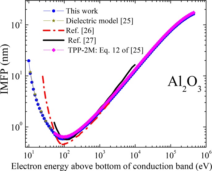
To validate our implementation, we reproduced the STPP²⁵ calculation of the IMFP for Al₂O₃ using the same input parameters (ω_min = E_g = 8.63 eV, ω_VB = 8.0 eV) and the same ELF data (kindly shared with us by S. Tanuma). Using these data, we obtained the IMFP results shown in Figure 1.

Figure 1.

IMFP for Al₂O₃ calculated in this work using the same input parameters and data used by Shinotsuka et al.²⁵

STPP tabulated their IMFP values rounded to three significant figures for incident electron kinetic energies (relative to the bottom of the conduction band) between 54.6 and 198789.2 eV at approximately 10% intervals. Our results when calculated at the same energies and likewise rounded to three significant figures agree exactly with theirs. For their graphed but untabulated results at energies below 50 eV, we compared our results to estimates digitized from their graph. We attribute the less than 1.5% difference to digitization error. Based on this close agreement, we believe that our implementation is, as intended, functionally the same as theirs, and we refer readers to their meticulous descriptions for details.

3. Energy-Loss Functions (ELF)

3.1. Optical-Data Acquisition

To compute the IMFP, optical data such as scattering factors, f₁ and f₂, refractive index n, and extinction index k have been collected from the literature.³⁹⁻⁴⁵Table 1 displays the data used to compute the ELF and the available parameters according to the published data.

Table 1. Data Collected for ELF Calculations.

material	energy range (eV)	optical constants	refs
liquid water	1.2398 × 10–7–6.1992	n and k	(39)
	6.2459–48.4	ϵ1 and ϵ2	(40)
	48.5814–10,701.0	δ and β	(41)
	11,032.1–432,945.1	f1 and f2	(42)
LiF	3.718 × 10–8–27.0	n and k	(43)
	29.3–10,917.6	δ and β	(41)
	11,032.1–432,945.1	f1 and f2	(42)
CaF2	0.0124–31.0	n and k	(44)
	31.7–10,920.5	δ and β	(41)
	11,032.1–432,945.1	f1 and f2	(42)
Al2O3	0.0372–27.0	n and k	(45)
	30.0–10644.4	δ and β	(41)
	11,032.1–432,945.1	f1 and f2	(42)

The dielectric function may be expressed with real and complex components as

4

In the optical limit of q→0,

5

and

6

where ϵ₁ represents the polarization term as a consequence of the interaction between the material and the electromagnetic wave, and ϵ₂ is the imaginary part, which is related to the energy loss.

It is also known that the interaction between photons and matter can be described in terms of the refractive index decrement, δ, and extinction coefficient, β, as⁴⁶

7

In eq 7, δ is related to the real atomic-scattering factor f₁, which represents the dispersive interaction between the incoming plane wave and the material, while β is related to the imaginary part of the atomic scattering factor f₂ that accounts for radiation absorption. In the limit of δ ≪ 1 and β ≪ 1 (e.g., energies above 100–200 eV, depending on the material), δ and β are approximated by⁴⁶

8

9

Otherwise⁴⁷

10

11

where N_A is Avogadro’s constant, r_e is the classical electron radius, λ is the incident wavelength, and f₁ and f₂ represent the real and complex components of the atomic-scattering factor of a given atom, respectively. f₁ and f₂ of a compound are the sum of the composition number of atoms in the compound’s molecular formula. In this work, eqs 8 and 9 were used for data above 11 keV.

The energy-loss function (ELF) can be written as

12

Due to the integration limits of the IMFP calculation (eq 2), information about the band-gap energy, the valence band width, and the minimum energy limit for each compound is required. Such information is given in Table 2.

Table 2. Bandgap and Valence Band Width (eV).

compound	Eg	ωVB	ωmin
liquid water	8.448	11.849	6.24
LiF	14.250	3.951	11.7
CaF2	12.152	5.8453	10.33
Al2O3	8.854	8.354	8.63

3.2. Optical-Data Evaluation

To evaluate the consistency of the ELF data, two mathematical rules were applied: Kramers–Kronig sum (KK-sum) and Bethe sum (f-sum). These two methods are indicators of the reliability of the optical data. The f-sum more strongly weights high energies while the KK-sum the low ones. According to Tanuma et al.,¹⁹ the KK-sum integration is influenced mainly by optical data in the energy range below 50 eV and the f-sum by data above. The mathematical representation of the KK-sum(55,56) is

13

In this work, n(0) was evaluated as the square root of the dielectric constant of each material.

The Bethe sum (f-sum) evaluates the number of electrons per atom or molecule that participate in the inelastic scattering process and is mathematically expressed as^57,58

14

where N is the atomic or molecular density, m_e is the electron mass, and ϵ₀ is the permittivity of free space. In eqs 13 and 14, ω_max is the maximum energy that we take to be 1 MeV. In the limit of ω_max → ∞, Z_eff → Z, and P_eff → 1.

The selection of the best ELF data was done through a thorough and rigorous evaluation process. To do that, we calculated the KK-sum and f-sum errors for each compound using different combinations of optical data sources. We selected the combination listed in Table 1, where the KK-sum and f-sum errors were the smallest. Table 3 displays the different compounds studied in this work with the associated f-sum and KK-sum errors. The lower the f-sum and KK-sum errors are, the better the internal consistency of the data. The data in Table 3 suggest an acceptable consistency between the different experimental results collected from the literature, mainly for liquid water and Al₂O₃. For Al₂O₃, the magnitude of our f-sum error is somewhat larger than that of Shinotsuka et al.,²⁵ 3.16% in this work versus −1.2%, while our KK-sum error was more than a factor of 2 better, 3.8% versus −7.8%. For liquid water, the f-sum and KK-sum results are 0.21% vs 5.1% and 2.7% vs 3.7% from reference (23), respectively. This result agrees quite well with the significant qualitative and quantitative improvement expected when using the revised data provided by NIST.⁴² Comparing data in Table 3 for the different compounds, the ELF for LiF has the highest error. However, the 13% KK-sum error obtained in this work is less than half of the 30% reported in the previous study.¹⁹ Furthermore, both f-sum and KK-sum errors are substantially smaller than the 34.7 and 24.3%, respectively, as reported by Boutboul and colleagues.²⁸ Regarding CaF₂, the ELF data can be considered reasonably accurate with f-sum and KK-sum errors of 2.4 and 5.8%, respectively.

Table 3. KK-sum and f-sum Errors.

compound	n(0)	Z	Zeff	f-sum error (%)	Peff	KK-sum error (%)
H2O	8.97	10	10.021	0.21	1.027	2.7
LiF	3	12	13.16	9.69	1.132	13.2
CaF2	2.6	38	38.91	2.4	1.058	5.8
Al2O3	3.13	50	51.58	3.16	1.038	3.8

4. Results

4.1. Energy-Loss Function

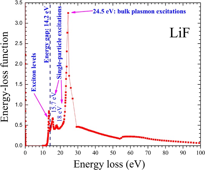
Our results for the energy-loss function are shown in Figure 2. As observed, all the materials typically have several local maxima and minima. These are related to increases or decreases in the inelastic-scattering probability. They are caused by physical phenomena such as inner shell excitations, valence electron excitations, plasmons, and excitons. Figure 2d also shows the ELF data used by Tanuma and collaborators⁴⁷ for Al₂O₃. Excellent agreement can be seen at energies greater than 30 eV. However, at lower energies, differences are observed, which can be associated with the use of new optical data in this work as compared to those by Tanuma and collaborators as explained above.

Figure 2.

ELFs for (a) liquid water, (b) LiF, (c) CaF₂, and (d) Al₂O₃. The insets show the ELF close to the energy gap.

4.2. Inelastic Mean Free Path

The IMFPs for liquid water, LiF, CaF₂, and Al₂O₃ as a function of the electron kinetic energy obtained through eq 2 and using input parameters from Table 2 and ELF data from Figure 2 are shown in Figures 3, 4, 5, and 6, respectively.

Figure 3.

IMFP for liquid water compared to reported results.

Figure 4.

IMFP for LiF compared to reported results and from the use of the TPP-2M formula.

Figure 5.

IMFP for CaF₂ compared with those from the TPP-2M formula.

Figure 6.

IMFP for Al₂O₃ compared to reported results and those from the TPP-2M formula.

The numerical values of the IMFPs are given in Table 4. Note that, regardless of the material, the IMFP initially diminishes with increasing energy to a broad minimum and then increases as the energy continues to increase.

Table 4. Calculated IMFP Values versus Energy Relative to the Bottom of the Conduction Band^a.

	IMFP (nm)
energy (eV)	liquid water	LiF	CaF2	Al2O3
10.0	10.2			19.7
11.0	7.64			11.1
12.2	5.95		17.0	7.49
13.5	4.78		10.2	5.47
14.9	3.94	8.61	7.08	4.20
16.4	3.31	5.83	5.32	3.36
18.2	2.83	4.33	4.14	2.76
20.1	2.45	3.41	3.33	2.30
22.2	2.14	2.78	2.76	1.95
24.5	1.89	2.31	2.34	1.68
27.1	1.69	1.91	2.01	1.46
30.0	1.53	1.62	1.74	1.29
33.1	1.39	1.40	1.53	1.15
36.6	1.28	1.24	1.35	1.04
40.4	1.20	1.12	1.22	0.942
44.7	1.13	1.02	1.12	0.858
49.4	1.08	0.941	1.05	0.777
54.6	1.04	0.837	0.990	0.705
60.3	1.01	0.759	0.941	0.651
66.7	0.996	0.713	0.901	0.618
73.7	0.989	0.690	0.870	0.599
81.5	0.990	0.678	0.848	0.588
90.0	0.998	0.674	0.828	0.583
99.5	1.01	0.676	0.810	0.585
109.9	1.04	0.684	0.797	0.591
121.5	1.07	0.697	0.793	0.602
134.3	1.10	0.714	0.799	0.618
148.4	1.15	0.736	0.814	0.637
164.0	1.20	0.760	0.836	0.661
181.3	1.26	0.788	0.865	0.689
200.3	1.32	0.821	0.900	0.720
221.4	1.40	0.858	0.941	0.755
244.7	1.48	0.900	0.987	0.794
270.4	1.57	0.947	1.04	0.837
298.9	1.67	1.00	1.10	0.884
330.3	1.78	1.06	1.16	0.935
365.0	1.90	1.12	1.24	0.992
403.4	2.04	1.20	1.32	1.05
445.9	2.18	1.28	1.40	1.12
492.7	2.34	1.36	1.50	1.20
544.6	2.52	1.46	1.61	1.28
601.8	2.70	1.57	1.72	1.37
665.1	2.91	1.68	1.85	1.46
735.1	3.14	1.81	1.99	1.57
812.4	3.38	1.94	2.14	1.69
897.8	3.65	2.09	2.30	1.81
992.3	3.94	2.26	2.48	1.95
1096.6	4.26	2.44	2.67	2.10
1212.0	4.61	2.63	2.88	2.27
1339.4	4.99	2.84	3.11	2.44
1480.3	5.40	3.07	3.36	2.64
1636.0	5.85	3.32	3.63	2.85
1808.0	6.34	3.60	3.93	3.09
1998.2	6.87	3.90	4.25	3.34
2208.3	7.45	4.22	4.60	3.61
2440.6	8.08	4.57	4.98	3.91
2697.3	8.77	4.96	5.40	4.24
2981.0	9.52	5.38	5.85	4.59
3294.5	10.3	5.83	6.34	4.98
3641.0	11.2	6.33	6.88	5.40
4023.9	12.2	6.87	7.46	5.86
4447.1	13.2	7.46	8.10	6.36
4914.8	14.4	8.10	8.79	6.90
5431.7	15.6	8.80	9.54	7.49
6002.9	17.0	9.55	10.4	8.13
6634.2	18.5	10.4	11.3	8.83
7332.0	20.1	11.3	12.2	9.59
8103.1	21.8	12.3	13.3	10.4
8955.3	23.7	13.3	14.4	11.3
9897.1	25.8	14.5	15.7	12.3
10938.0	28.1	15.7	17.0	13.4
12088.4	30.5	17.1	18.5	14.5
13359.7	33.2	18.6	20.1	15.8
14764.8	36.1	20.2	21.8	17.1
16317.6	39.2	21.9	23.7	18.6
18033.7	42.6	23.8	25.7	20.2
19930.4	46.2	25.8	27.9	21.9
22026.5	50.2	28.0	30.3	23.7
24343.0	54.5	30.4	32.8	25.8
26903.2	59.1	33.0	35.6	27.9
29732.6	64.1	35.7	38.6	30.3
32859.6	69.5	38.7	41.8	32.8
36315.5	75.2	41.9	45.2	35.5
40134.8	81.5	45.3	48.9	38.4
44355.9	88.1	49.0	52.9	41.5
49020.8	95.2	52.9	57.1	44.8
54176.4	103	57.1	61.7	48.4
59874.1	111	61.6	66.5	52.2
66171.2	119	66.4	71.6	56.2
73130.4	129	71.4	77.0	60.4
80821.6	138	76.7	82.7	64.9
89321.7	148	82.3	88.7	69.6
98715.8	159	88.1	95.0	74.6
109097.8	170	94.3	102	79.7
120571.7	181	101	108	85.1
133252.4	193	107	116	90.7
147266.6	206	114	123	96.5
162754.8	218	121	130	102
179871.9	231	128	138	108
198789.2	245	135	146	115
219696.0	258	143	154	121
242801.6	271	150	162	127
268337.3	285	158	170	133
296558.6	298	165	178	139
327747.9	311	172	185	145
362217.4	324	179	193	151
400312.2	336	186	200	157
432945.1	345	191	206	162

^aNote that, if desired, the scattering cross sections (σ) can be computed from the IMFP values (λ) using the formula λ^–1 = Nσ and the following values of N: (3.34,6.12,2.45,2.34) × 10²²/cm³ for liquid H₂O, LiF, CaF₂, and Al₂O₃ respectively.

Also shown in Figures 3, 4, and 6 are the IMFP data reported in the literature. Relatively good agreement can be observed at energies greater than 200 eV. Note that Figures 4, 5, and 6 include IMFP calculations using the TPP-2M formula. As can be seen, qualitative agreement is obtained.

5. Discussion

From the IMFP data for Al₂O₃ shown in Figure 1, we see that when we use the same ELF (Figure 2d) as STPP,²⁵ we reproduce exactly their result. However, our best estimates for the ELF data and other input parameters differ somewhat from theirs, leading to the differences shown in Figure 6. We restrict the comparison to energies greater than or equal to 54.6 eV, above which Shinotsuka et al. tabulated their data. At energies greater than 200 eV, our IMFP values are about 7.5% smaller than theirs, but at energies below 200 eV, the difference increases to approximately 9%. The smaller difference at the higher energies is likely associated with differences in the ELF, whereas the larger difference at lower energies reflects sensitivity to the band gap and minimum integration limit.

Comparing our results for liquid water shown in Figure 3 with updated data reported by Shinotsuka et al.,²⁵ a difference of 2.5% is observed at energies greater than 150 eV and varies from 0.02 to 1.4% at energies between 40 and 150 eV. Below 40 eV, differences from 1.3% up to 29% are found, being larger at lower energies. Reference (23) was published before Shinotsuka et al. began modeling the effect of the band gap, and the lower integration limit was set to zero.⁴⁷ However, for the updated data reported in ref (25), the Boutboul’s energy gap treatment was considered, and the lower integration limit was set to E_g = 7.9 eV. The 2.5% difference at high energies appears to be mainly attributable to differences in the ELF data. The larger differences (up 29%) at low energies are associated with the sensitivity to the band gap and its effect on the integration limits.

As mentioned above, the TPP-2M formula²⁰ has been proposed to calculate the IMFP for LiF and other inorganic compounds for which data are not available.²⁵ In order to use this formula, four parameters are required. Thus, in this work, we also calculated the IMFP for LiF, CaF₂, and Al₂O₃ through the relativistic TPP-2M formula by using equation 12 from ref (25). The LiF parameters came from Table 7 of ref (19), but for Al₂O₃, we used parameters reported in Table 6 of ref (25). For CaF₂, equations 15a–15e of ref (25) were used. We used the band gap from Table 2 of this work, while the plasmon energy and the number of valence electrons per molecule were obtained elsewhere.⁵⁹ These results are shown in Figures 4, 5, and 6 for LiF, CaF₂, and Al₂O₃, respectively. As can be noted, qualitative agreements are seen between our results and the results of the TPP-2M formula. The differences (approximately −10% at energies below 200 eV and −7.35% above) between our and STPP’s results for Al₂O₃ using the dielectric FPA are reproduced by the TPP-2M formula. For CaF₂, the difference is nearly constant at −21% for energies over 200 eV and varies between −17 and 0.21% at lower energies. For LiF, the average differences are around −4% at energies above 200 eV and vary from 5 to 34% at energies below. In contrast, despite the remarkable difference between the ELF KK-sum errors obtained in this work and that of ref (19), the differences in input parameters, and the band-gap treatment, the IMFP values obtained for LiF differ from that paper’s dielectric-function theory results only by −7% in the 200–2000 eV energy range. Larger differences are evident in Figure 4 at low energies, but the TPP-2M equation was claimed to be reliable at energies above 200 eV.²⁵

Regarding the data for liquid water published by Emfietzoglou et al.,^6,11 differences of up to 186% in the IMFPs are found for the e-e model at energies below 100 eV. At higher energies, the disagreements in the IMFPs vary from 2% up to 18% and between 0.7 and 46% for the e-e and IXS-D3 models, respectively. As mentioned by Shinotsuka et al.,²³ these differences can be explained as consequences of the inclusion of exchange and correlation effects and the use of a ϵ₂(ω) fit instead of the ELF data.^6,11 As seen in Figure 3, the IMFP data from Akkerman and Akkerman²⁹ are very close to those from Emfietzoglou’s e-e model. Similar differences from 19 to 129% are obtained at energies below 100 eV and 2% at energies above when compared to our results. The IMFP data at energies between 20 and 100 eV for liquid water reported by Garcia-Molina et al.³¹ and de Vera and Garcia-Molina³³ are greater than ours by 7–21% and 15–20%, respectively, while those from Nguyen-Truong³² are greater by 6–16% in the energy range from 35 to 100 eV and smaller by 2.5–30% at energies down to 20 eV. At higher energies, the differences are found to be 1.9%, 0.8%, and from 0.06 to 15%, respectively. Contrary to data from refs (6)(11), and (29), the results recently published by Garcia-Molina et al.^31,33 and Nguyen-Truong³² show smaller differences compared to our results at energies between 20 and 100 eV. The differences observed at low energies between our IMFPs and those reported in refs (31, 33) could presumably be interpreted as a consequence of the ELF data sets used for the dielectric-function calculation, which is very sensitive to the optical data, or due to the inclusion of higher-order corrections to the first-Born approximation and/or the integration limit³³ as mentioned above. For example, Garcia-Molina et al.³¹ used a Mermin energy-loss-function–generalized-oscillator-strength (MELF-GOS) model for describing the ELF in their method, Akkerman and Akkerman²⁹ used a Drude-type variation for the ELF construction, and Nguyen-Truong³² considered an ELF based on a Mermin–Levine–Louie (MLL) dielectric function.

Considering the results for Al₂O₃ published by Pandya et al.²⁶ and Akkerman et al.,²⁷ differences of up to 270 and 57% in the IMFPs are obtained, respectively, at energies below 100 eV. At higher energies, the reported IMFPs differ from this work by around 6–20%²⁶ and 0.3–35%,²⁷ respectively. The observed difference between our results and the data published by Akkerman et al.²⁷ could be due to the combination of the dielectric theory with a classical binary-encounter approximation used in their work. With respect to Pandya et al.,²⁶ the difference can be associated with the semiempirical quantum-mechanical method used to obtain the atomic molecular inelastic cross section.

As is evident from the above discussion, there is variation among reported calculated IMFP values, relatively small at high energies, but several tens of percent at energies below 50 eV. Some of the variation is due to uncertainties in the modeling, for example, use of the Born approximation (a high-energy approximation) in the derivation of eq 1, the choice of extension model (e.g., Mermin or Lindhard components, discrete or continuous) to extend available ELF(0, ω) to ELF(q > 0, ω), and the choice of whether to include exchange and correlation effects or not, and if so, how. The choice of extension algorithm can make a difference of 5% at 10 keV and 25% at 50 eV.^11,60 Exchange and correlation effects can be in the range of from −2 to +15% at 10 keV and from −15 to +35% at 50 eV.¹¹

The errors in the IMFP associated with input parameters such as the band-gap and valence band-width energies have been assessed. Considering the variation of the data reported in the literature, we estimated the best values of these parameters to within 1 eV. We found that the maximum errors associated with the valence band width to be approximately 2.3, 2.1, 1.6, and 3.3% for liquid water, LiF, CaF₂, and Al₂O₃, respectively, at energies below 100 eV, while those related to the energy gap were 1.2, 0.0014, 0.007, and 0.28%, respectively. As observed, the errors due to the valence band width are greater than those related to the band-gap energy. The results indicate that these errors are not so important relative to the model uncertainties described above.

6. Conclusions

In this work, the electron inelastic mean free path for LiF, CaF₂, Al₂O₃, and liquid water has been investigated from 443 keV down to the energy gap. The calculation was performed using the dielectric-function model through the relativistic full Penn algorithm (FPA). An integration limit that accounts for the band-gap, the valence band width, and the exciton interactions has been established. The results suggest that, at electron energies below 100 eV, the different choices of models for integration limits can affect the IMFP by up to 29% and the exciton interaction by ∼9%. At energies greater than 100 eV, the difference between our results and those from STPP²⁵ for Al₂O₃ is around 7.5%, which is associated with choice of the ELF and other input parameters.

The authors declare no competing financial interest.

References

- Martin F.; Burrow P. D.; Cai Z.; Cloutier P.; Hunting D.; Sanche L. DNA Strand breaks induced by 0–4 eV electrons: the role of shape resonances. Phys. Rev. Lett. 2004, 93, 068101 10.1103/PhysRevLett.93.068101. [DOI] [PubMed] [Google Scholar]
- Massillon-JL G.; Cabrera-Santiago A.; Minniti R.; O’Brien M.; Soares C. G. Influence of phantom materials on the energy dependence of LiF:Mg,Ti thermoluminescent dosimeters exposed to 20-300 kV narrow x-ray spectra, 137Cs and 60Co photons. Phys. Med. Biol. 2014, 59, 4149–4166. 10.1088/0031-9155/59/15/4149. [DOI] [PubMed] [Google Scholar]
- Cabrera-Santiago A.; Massillon-JL G.. Secondary electron fluence generated in LiF:Mg, Ti by low-energy photons and its contribution to the absorbed dose. AIP Conference Proc.: AIP Publishing: 2016, 1747, 020004. [Google Scholar]
- Massillon-JL G.; Cabrera-Santiago A.; Xicohténcatl-Hernández N. Relative efficiency of Gafchromic EBT3 and MD-V3 films exposed to low-energy photons and its influence on the energy dependence. Physica Medica 2019, 61, 8–17. 10.1016/j.ejmp.2019.04.007. [DOI] [PubMed] [Google Scholar]
- Cabrera-Santiago A.; Massillon-JL G. Track-average LET of secondary electrons generated in LiF:Mg,Ti and liquid water by 20–300 kV x-ray, 137Cs and 60Co beams. Phys. Med. Biol. 2016, 61, 7919–7933. 10.1088/0031-9155/61/22/7919. [DOI] [PubMed] [Google Scholar]
- Emfietzoglou D.; Nikjoo H. Accurate electron inelastic cross sections and stopping powers for liquid water over the 0.1–10 keV range based on an improved dielectric description of the Bethe surface. Radiat. Res. 2007, 167, 110–120. 10.1667/RR0551.1. [DOI] [PubMed] [Google Scholar]
- Kyriakou I.; Incerti S.; Francis Z. Technical note: improvements in GEANT4 energy-loss model and the effect on low-energy electron transport in liquid water. Med. Phys. 2015, 42, 3870–3876. 10.1118/1.4921613. [DOI] [PubMed] [Google Scholar]
- Fernández-Varea J. M.; Salvat F.; Dingfelder M.; Liljequist D. A relativistic optical-data model for inelastic scattering of electrons and positrons in condensed matter. Nucl. Instrum. Methods. Phys. Res., Sect. B 2005, 229, 187–218. 10.1016/j.nimb.2004.12.002. [DOI] [Google Scholar]
- Emfietzoglou D.; Moscovitch M. Inelastic collision characteristics of electrons in liquid water. Nucl. Instrum. Methods. Phys. Res., Sect. B 2002, 193, 71–78. 10.1016/S0168-583X(02)00729-2. [DOI] [Google Scholar]
- Emfietzoglou D.; Karava K.; Papamichael G.; Moscovitch M. Monte Carlo simulation of the energy loss of low-energy electrons in liquid water. Phys. Med. Biol. 2003, 48, 2355–2371. 10.1088/0031-9155/48/15/308. [DOI] [PubMed] [Google Scholar]
- Emfietzoglou D.; Kyriakou I.; Garcia-molina R.; Abril I. Inelastic mean free path of low-energy electrons in condensed media: beyond the standard models. Surf. Interface Anal. 2017, 49, 4–10. 10.1002/sia.5878. [DOI] [Google Scholar]
- Fernández-Varea J. M.; González-Muñoz G.; Galassi M. E.; Wiklund K.; Lind B. K.; Ahnesjö A.; Tilly N. Limitations (and merits) of PENELOPE as a track-structure code. Int. J. Radiat. Biol. 2011, 88, 66–70. 10.3109/09553002.2011.598209. [DOI] [PubMed] [Google Scholar]
- Villarrubia J. S.; Ding Z. J. Sensitivity of scanning electron microscope width measurements to model assumptions. J. Micro/Nanolithogr. MEMS MOEMS 2009, 8, 033003 10.1117/1.3190168. [DOI] [Google Scholar]
- Villarrubia J. S.; Vladár A. E.; Ming B.; Kline R. J.; Sunday D. F.; Chawla J. S.; List S. Scanning electron microscope measurement of width and shape of 10 nm patterned lines using a JMONSEL-modeled library. Ultramicroscopy 2015, 154, 15–28. 10.1016/j.ultramic.2015.01.004. [DOI] [PubMed] [Google Scholar]
- Powell C. J. Attenuation lengths of low-energy electrons in solids. Surf. Sci. 1974, 44, 29–46. 10.1016/0039-6028(74)90091-0. [DOI] [Google Scholar]
- Penn D. R. Electron mean-free-path calculations using a model dielectric function. Phys. Rev. B 1987, 35, 482–486. 10.1103/PhysRevB.35.482. [DOI] [PubMed] [Google Scholar]
- Tanuma S.; Powell C. J.; Penn D. R. Calculations of electron inelastic mean free paths for 31 materials. Surf. Interface Anal. 1988, 11, 577–589. 10.1002/sia.740111107. [DOI] [Google Scholar]
- Tanuma S.; Powell C. J.; Penn D. R. Proposed formula for electron inelastic mean free paths based on calculations for 31 materials. Surf. Sci. 1987, 192, L849–L857. 10.1016/S0039-6028(87)81156-1. [DOI] [Google Scholar]
- Tanuma S.; Powell C. J.; Penn D. R. Calculations of Electron Inelastic Mean Free Paths. III. Data for 15 Inorganic Compounds over the 50-2000 eV Range. Surf. Interface Anal. 1991, 17, 927–939. 10.1002/sia.740171305. [DOI] [Google Scholar]
- Tanuma S.; Powell C. J.; Penn D. R. Calculations of electron inelastic mean free paths. V. Data for 14 organic compounds over the 50–2000 eV range. Surf. Interface Anal. 1994, 21, 165–176. 10.1002/sia.740210302. [DOI] [Google Scholar]
- Powell C. J.; Jablonski A. Evaluation of electron inelastic mean free paths for selected elements and compounds. Surf. Interface Anal. 2000, 29, 108–114. 10.1002/(SICI)1096-9918(200002)29:2<108::AID-SIA700>3.0.CO;2-4. [DOI] [Google Scholar]
- Tanuma S.; Powell C. J.; Penn D. R. Calculations of electron inelastic mean free paths. IX. Data for 41 elemental solids over the 50 eV to 30 keV range. Surf. Interface Anal. 2011, 43, 689–713. 10.1002/sia.3522. [DOI] [Google Scholar]
- Shinotsuka H.; Da B.; Tanuma S.; Yoshikawa H.; Powell C. J.; Penn D. R. Calculations of electron inelastic mean free paths. XI. Data for liquid water for energies from 50 eV to 30 keV. Surf. Interface Anal. 2017, 49, 238–252. 10.1002/sia.6123. [DOI] [PMC free article] [PubMed] [Google Scholar]
- Shinotsuka H.; Tanuma S.; Powell C. J.; Penn D. R. Calculations of electron inelastic mean free paths. X. Data for 41 elemental solids over the 50 eV to 200 keV range with the relativistic full Penn algorithm. Surf. Interface Anal. 2015, 47, 871–888. 10.1002/sia.5789. [DOI] [Google Scholar]
- Shinotsuka H.; Tanuma S.; Powell C. J.; Penn D. R. Calculations of electron inelastic mean free paths. XII. Data for 42 inorganic compounds over the 50 eV to 200 keV range with the full Penn algorithm. Surf. Interface Anal. 2019, 51, 427–457. 10.1002/sia.6598. [DOI] [PMC free article] [PubMed] [Google Scholar]
- Pandya S. H.; Vaishnav B. G.; Joshipura K. N. Electron inelastic mean free paths in solids: A theoretical approach. Chin. Phys. B 2012, 21, 093402 10.1088/1674-1056/21/9/093402. [DOI] [Google Scholar]
- Akkerman A.; Boutboul T.; Breskin A.; Chechik R.; Gibrekhterman A.; Lifshitz Y. Inelastic electron interactions in the energy range 50 eV to 10 keV in insulators: Alkali halides and metal oxides. Phys. Status Solidi B 1996, 198, 769–784. 10.1002/pssb.2221980222. [DOI] [Google Scholar]
- Boutboul T.; Akkerman A.; Breskin A.; Chechik R. Electron inelastic mean free path and stopping power modelling in alkali halides in the 50 eV–10 keV energy range. J. Appl. Phys. 1996, 79, 6714–6721. 10.1063/1.361491. [DOI] [Google Scholar]
- Akkerman A.; Akkerman E. Characteristics of electron inelastic interactions in organic compounds and water over the energy range 20–10000 eV. J. Appl. Phys. 1999, 86, 5809–5816. 10.1063/1.371597. [DOI] [Google Scholar]
- Tanuma S.; Powell C. J.; Penn D. R. Calculations of Electron Inelastic Mean Free Paths (IMFPs). IV. Evaluation of Calculated IMFPs and of the Predictive IMFP Formula TPP-2 for Electron Energies between 50 and 2000 eV. Surf. Interface Anal. 1993, 20, 77–89. 10.1002/sia.740200112. [DOI] [Google Scholar]
- Garcia-Molina R.; Abril I.; Kyriakou I.; Emfietzoglou D. Inelastic scattering and energy loss of swift electron beams in biologically relevant materials. Surf. Interface Anal. 2017, 49, 11–17. 10.1002/sia.5947. [DOI] [Google Scholar]
- Nguyen-Truong H. T. Low-energy electron inelastic mean free paths for liquid water. J. Phys.: Condens. Matter 2018, 30, 155101. 10.1088/1361-648X/aab40a. [DOI] [PubMed] [Google Scholar]
- de Vera P.; Garcia-Molina R. Electron inelastic mean free paths in condensed matter down to a few electronvolts. J. Phys. Chem. C. 2019, 123, 2075–2083. 10.1021/acs.jpcc.8b10832. [DOI] [Google Scholar]
- Tanuma S.; Powell C. J.; Penn D. R. Calculation of electron inelastic mean free paths (IMFPs) VII. Reliability of the TPP-2M IMFP predictive equation. Surf. Interface Anal. 2003, 35, 268–275. 10.1002/sia.1526. [DOI] [Google Scholar]
- Bourke J. D.; Chantler C. T. Electron Energy Loss Spectra and Overestimation of Inelastic Mean Free Paths in Many-Pole Models. J. Phys. Chem. A. 2012, 116, 3202–3205. 10.1021/jp210097v. [DOI] [PubMed] [Google Scholar]
- Fano U. Penetration of protons, alpha particles, and mesons. Annu. Rev. Nucl. Sci. 1963, 13, 1–66. 10.1146/annurev.ns.13.120163.000245. [DOI] [Google Scholar]
- Samarin S.; Berakdar J.; Suvorova A.; Artamonov O. M.; Waterhouse D. K.; Kirschner J.; Williams J. F. Secondary-electron emission mechanism of LiF film by (e,2e) spectroscopy. Surf. Sci. 2004, 548, 187–199. 10.1016/j.susc.2003.11.003. [DOI] [Google Scholar]
- Abbamonte P.; Graber T.; Reed J. P.; Smadici S.; Yeh C.-L.; Shukla A.; Rueff J.-P.; Ku W. Dynamical reconstruction of the exciton in LiF with inelastic x-ray scattering. PNAS. 2008, 105, 12159–12163. 10.1073/pnas.0801623105. [DOI] [PMC free article] [PubMed] [Google Scholar]
- Querry M. R.; Wieliczka D. M.; Segelstein D. J.. Handbook of optical constants, Academic Press: 2,1991. [Google Scholar]
- Hayashi H.; Watanabe N.; Udagawa Y.; Kao C.-C. The complete optical spectrum of liquid water measured by inelastic x-ray scattering. PNAS. 2000, 97, 6264–6266. 10.1073/pnas.110572097. [DOI] [PMC free article] [PubMed] [Google Scholar]
- Henke B. L.; Gullikson E. M.; Davis J. C. X-ray interactions: photoabsorption, scattering, transmission, and reflection at E = 50-30,000 eV, Z = 1-92. At. Data Nucl. Data Tables 1993, 54, 181–342. 10.1006/adnd.1993.1013. [DOI] [Google Scholar]
- Chantler C. T.; Olsen K.; Dragoset R. A.; Chang J.; Kishore A. R.; Kotochigova S. A.; Zucker D. S.. X-ray form factor, attenuation and scattering tables (version 2.1) 2005, Available online at: http://physics.nist.gov/ffast (accessed 2018)
- Palik E. D.; Hunter W. R.. Handbook of Optical Constants. 1st ed. Academic Press: 1985; pp 35–68. [Google Scholar]
- Bezuidenhout D. F.; Handbook of optical constants. 2nd ed.; Academic Press: 1991; pp 815–835. [Google Scholar]
- William J.; Thomas M. E.. Handbook of optical constants. 3rd ed.; Academic Press, 1998; pp 653–663. [Google Scholar]
- Piegary A; Flory F.. Optical thin films and coatings .1st ed.; Woodhead Publishing Limited: 2013; pp 1–845. [Google Scholar]
- Tanuma S.Private communication, 2019.
- Shimkevich A. Electrochemical View of the Band Gap of Liquid Water for Any Solution. World J. Condens. Matter Phys. 2014, 04, 243–249. 10.4236/wjcmp.2014.44027. [DOI] [Google Scholar]
- Winter B.; Weber R.; Widdra W.; Dittmar M.; Faubel M.; Hertel I. V. Full Valence Band Photoemission from Liquid Water Using EUV Synchrotron Radiation. J. Phys. Chem. A. 2004, 108, 2625–2632. 10.1021/jp030263q. [DOI] [Google Scholar]
- Poole R. T.; Liesegang J.; Leckey R. C. G.; Jenkin J. G. Electronic band structure of the alkali halides. II. Critical survey of theoretical calculations. Phys. Rev. B 1975, 11, 5190–5196. 10.1103/PhysRevB.11.5190. [DOI] [Google Scholar]
- Massillon-JL G.; Johnston C. S. N.; Kohanoff J. On the role of magnesium in a LiF:Mg,Ti thermoluminescent dosimeter. J. Phys.: Condens. Matter. 2019, 31, 025502 10.1088/1361-648X/aaee62. [DOI] [PubMed] [Google Scholar]
- Cadelano E.; Cappellini G. Electronic structure of fluorides: General trends for ground and excited state properties. Eur. Phys. J. B 2011, 81, 115–120. 10.1140/epjb/e2011-10382-1. [DOI] [Google Scholar]
- Scrocco M. Satellites in x-ray photoelectron spectroscopy of insulators. I. Multielectron excitations in CaF2,SrF2, andBaF2. Phys. Rev. B 1985, 32, 1301–1305. 10.1103/PhysRevB.32.1301. [DOI] [PubMed] [Google Scholar]
- Perevalov T. V.; Shaposhnikov A. V.; Gritsenko V. A.; Wong H.; Han J. H.; Kim C. W. Electronic Structure of α-Al2O3: Ab Initio Simulations and Comparison with Experiment. JETP Lett. 2007, 85, 165–168. 10.1134/S0021364007030071. [DOI] [Google Scholar]
- Fisher K., Daniels J., Hess S.; Tracts in modern physics. 1st ed.; Springer- Verlag: Alemania, 1970; pp 1–72. [Google Scholar]
- Wooten F.; Optical Properties of Solids. 1st ed.; Academic Press: California, 1972; pp 1–255. [Google Scholar]
- Egerton R. F.; Electron Energy-Loss Spectroscopy in the Electron Microscope, 3rd ed.; Springer:, 2011; pp 1–485. [Google Scholar]
- Bethe H. A.; Morrison P.; Ford K. W.. Elementary Nuclear Theory, 1st ed.; John Wiley and Sons: New York, 1947; pp 1–141. [Google Scholar]
- Powell C. J.; Jablonski A.. NIST Electron Inelastic-Mean-Free-Path Database. 2010. Available at https://www.nist.gov/sites/default/files/documents/srd/SRD71UsersGuideV1-2.pdf
- Da B.; Shinotsuka H.; Yoshikawa H.; Tanuma S. Comparison of the Mermin and Penn models for inelastic mean-free path calculations for electrons based on a model using optical energy-loss functions. Surf. Interface Anal. 2019, 51, 627–640. 10.1002/sia.6628. [DOI] [Google Scholar]