Local field potentials in dorsal anterior cingulate sulcus reflect rewards but not travel time costs during foraging

Abstract

To maximise long-term reward rates, foragers deciding when to leave a patch must compute a decision variable that reflects both the immediately available reward and the time costs associated with travelling to the next patch. Identifying the mechanisms that mediate this computation is central to understanding how brains implement foraging decisions. We previously showed that firing rates of dorsal anterior cingulate sulcus neurons incorporate both variables. This result does not provide information about whether integration of information reflected in dorsal anterior cingulate sulcus spiking activity arises locally or whether it is inherited from upstream structures. Here, we examined local field potentials gathered simultaneously with our earlier recordings. In the majority of recording sites, local field potential spectral bands – specifically theta, beta, and gamma frequency ranges – encoded immediately available rewards but not time costs. The disjunction between information contained in spiking and local field potentials can constrain models of foraging-related processing. In particular, given the proposed link between local field potentials and inputs to a brain area, it raises the possibility that local processing within dorsal anterior cingulate sulcus serves to more fully bind immediate reward and time costs into a single decision variable.

Introduction

Foraging describes the process by which animals actively search for and harvest resources (Stephens and Krebs, 1986). While foraging, animals must decide whether to accept or reject a particular item upon encounter and choose when to leave a depleting patch of resources for a better one. Foraging behaviour is ubiquitous and manifests in varied contexts including foraging for water, sexual opportunities, social encounters, and even information (Dukas, 2002; Fu and Pirolli, 2007; Pirolli, 2007; Stephens and Krebs, 1986). Moreover, the foraging framework has been extended beyond physical resources to understand cognitive concepts like visual search (Anderson et al., 2013; Cain et al., 2012; Wolfe, 2018), free recall (Hills et al., 2012, 2015), social processing (Hills and Pachur, 2012), and problem solving (Hills et al., 2010; Payne and Duggan, 2011), suggesting that foraging computations are a neurological primitive and central to a wide array of cognitive functions (Hills et al., 2010; Newell, 1992).

The computational demands of foraging for dispersed and difficult to obtain resources have been hypothesised to be a major contributor to the rapid development of the human neocortex (DeCasien et al., 2017; Genovesio et al., 2014; González-Forero and Gardner, 2018; Milton, 1988). Despite the central importance of foraging for understanding behaviour, the neural circuits that mediate foraging have only recently begun to be described (Barack et al., 2017; Daw et al., 2006; Hayden et al., 2011; Kolling et al., 2012; Strait et al., 2014). In mammals, the main cortical nodes of the putative foraging circuit include ventromedial prefrontal cortex (vmPFC), anterior cingulate cortex (ACC), and posterior cingulate cortex (PCC; Heilbronner and Hayden, 2016; Vogt et al., 1979). The activity of these nodes is regulated by dopamine (Björklund and Dunnett, 2007; Williams and Goldman-rakic, 1993) and norepinephrine (Aston-Jones and Cohen, 2005).

Foraging decisions typically require animals to accept or reject foreground choices based on the immediately available reward. Choosing whether to accept or reject an option is thought to be mediated by two distinct valuation processes: one related to valuation of the immediately available foreground options, carried out by the vmPFC (Kolling et al., 2012; McGuire and Kable, 2015; Shenhav et al., 2014; Strait et al., 2014). The other valuation process involves estimation of the background context, including the local history of rewards and cost of travelling, and appears to be mediated by the dorsal anterior cingulate sulcus (dACC) (Blanchard et al., 2015; Hayden et al., 2011; Kolling et al., 2012; Shenhav et al., 2014; Wittmann et al., 2016). Decisions in these contexts also require integrating accept and reject computations over multiple decisions, a strategic process associated with PCC (Barack et al., 2017).

In a previous study (Hayden et al., 2011), we showed that spike rates of dorsal ACC (dACC) neurons vary with both immediately available reward and time costs of travelling from patch to patch, the two key variables the animals must track to in order to maximize their intake rates. However, whether the activity observed in dACC neurons is a result of local processing or reflects signals inherited from other brain areas upstream to dACC is unclear. To address this question, we examined local field potentials (LFPs) gathered simultaneously with neuronal spiking activity from the same recordings in dACC (Hayden et al., 2011). LFPs are thought to index dendritic potentials reflecting the inputs to a given cortical area, as well as local circuit processes, whereas spikes are thought to index outputs of a brain area (Buzsáki et al., 2012; Einevoll et al., 2013; Mitzdorf, 1985; Monosov et al., 2008; Sendhilnathan et al., 2017). We hypothesised that if LFPs in dACC differ from spiking activity at the same sites, by reflecting only reward or time costs but not both, this would endorse a role for dACC in integrating immediate reward and time costs into a single decision variable during patch foraging.

Here we report evidence in favour of dACC’s role in cost–benefit computations. Modulations of LFP power spectra, especially in theta, beta, and gamma frequency bands, robustly encoded immediately available reward at several sites. LFPs from few sites signalled time costs. Furthermore, simultaneously recorded dACC spiking activity strongly encoded reward value modulated by time costs. Together, these observations suggest dACC receives reward-related inputs which are locally combined with signals reflecting time costs in order to generate spike rates signal reward value normalised by time costs. The source of time costs, how they are transmitted to dACC, and how they are integrated with reward signals, however, remains unknown.

Results

Monkeys forage optimally in a virtual patch foraging task

The patch foraging task has been described in detail previously (Blanchard and Hayden, 2015; Hayden et al., 2011). In this task, on any given trial, the animal faced two options: choosing (by shifting gaze) the ‘stay’ option, represented by the short blue target (Figure 1(a)), led to a juice reward after a short delay (called handling time, 0.4 s). The juice reward began at a high value (306 µL) and declined by 19 ± 1.9 µL each time the animal chose the stay option (Figure 1(b)). On the other hand, choosing the ‘leave’ option, represented by the tall grey target, led to no reward and a long delay. At the end of the delay period, the value of the stay target was reset to the high initial value (i.e. 306 µL). Time spent choosing the stay option (time in the patch) is referred to as ‘patch residence time’. The long delay after the animal chose to leave the patch is referred to as ‘travel time’. Travel time was indicated by the height of the grey bar and was chosen randomly from a uniform distribution (0.5–10.5 s), and changed only following decisions to leave a patch.

Figure 1.

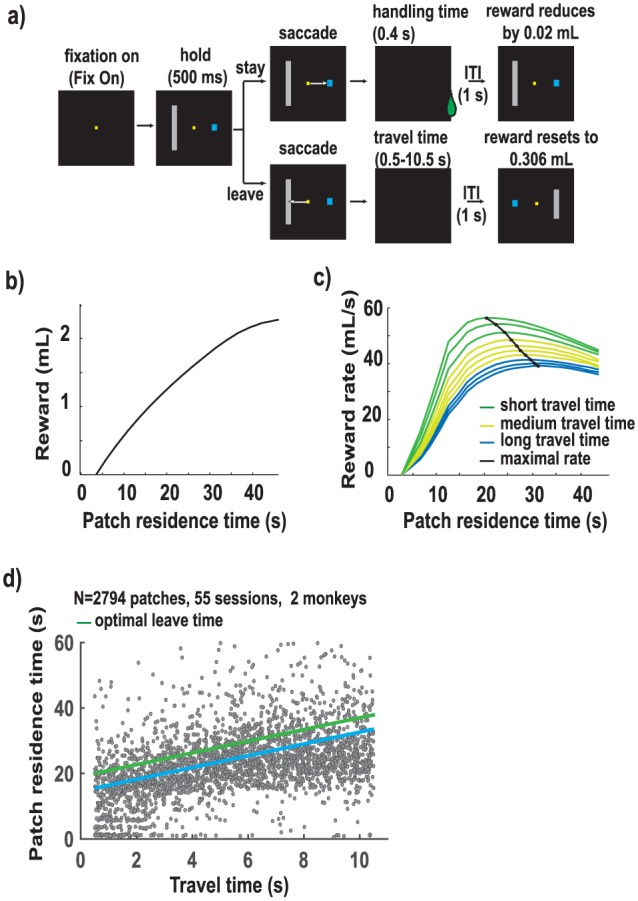
Patch-leaving task ((a)–(c), adapted with permission from Hayden et al., 2011)). (a) Task design. After fixation, two eccentric targets, a large grey and a small blue rectangle, appear. Monkey chooses one of two targets by shifting gaze to it. Choice of blue rectangle (stay in patch) yields a short delay (0.4 s, handling time) and reward whose value diminishes by 19 μL per trial. Choice of grey rectangle (leave patch) yields no reward and a long delay (travel time) whose duration is indicated by the height of the bar and resets the value of the blue rectangle at 306 μL. Travel time varies randomly from patch to patch and ranges from 0.5 to 10.5 s. (b) Plot of the cumulative reward available in this task as a function of time in patch (black line). (c) Plot of reward intake rate derived from a range of patch residence times (x-axis). Data are shown for each of 10 travel times (1-s intervals from 0.5 to 10.5 s). Rate-maximising time in patch (the curves’ maxima, shown by the black line) increases with increasing travel time. Data are generated based on average times associated with actual animal performance. (d) Monkeys performed optimally in the patch-leaving task: Monkeys remain in the patch longer as travel time rises, as predicted by the marginal value theorem (MVT). Each dot indicates a single patch-leaving decision (n = 2794 patch-leaving events). The time at which the monkey chose to leave the patch (y-axis) was defined relative to the beginning of foraging in that patch. Travel time was kept constant in a patch (x-axis). Data from both monkeys are shown. Average leave time is shown by the blue trace, MVT-prescribed optimal leave time in green.

The marginal value theorem (MVT; Charnov, 1976) – the normative model in these conditions– prescribes that the animal should leave a patch when the instantaneous reward rate falls below the average reward rate for the environment. When the travel delay is larger, the average reward rate reduces, and the animal should stay in the patch longer. Consistent with this prediction, in our data, we observed a significant increase in patch residence time with increase in travel time (Figure 1(d); Pearson’s r = 0.32, p < 0.0001). Furthermore, the two monkeys performed nearly optimally: the average deviation from optimal leave time was <3 s. Put another way, the animals obtained >95% of the maximum reward obtainable as predicted by the MVT, given certain assumptions about variability in their behaviour (see Hayden et al., 2011 for details).

Patch residence time weakly modulates event-related LFPs

The neural data presented here were recorded from 55 sites in dACC from two monkeys performing the patch foraging task (27 sites in monkey E, 28 in monkey O). Event-related potentials (ERPs) were determined by aligning them to the onset of fixation, when the patches appeared (left column in Figure 2.), and to the end of the choice saccade (right column in Figure 2). ERPs for the example site (Figure 2(a)) and the aggregate ERPs across sites (Figure 2(b)) show that the dACC field potentials decrease in voltage just prior to the trial and around the time of the choice saccade, then increase as the time of reward delivery approaches. Decrease in ERPs around the time of the choice saccade followed by an increase in anticipation of reward is consistent with observations from a previous report (Emeric et al., 2008).

Figure 2.

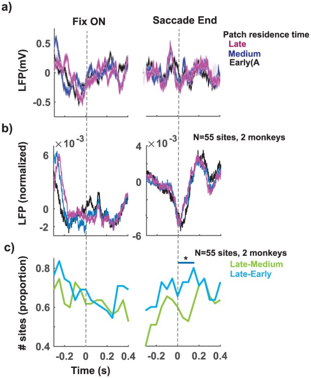
Influence of patch residence time on event-related field potentials (ERPs). Phasic increase in dACC ERPs were observed after stimulus onset (left panel, Fix ON) and around the time of the saccade (right panel, saccade end) at an example site (a) and for the normalised aggregate LFPs across sites (N = 55, 2 monkeys) in (b) during a ‘stay’ trial at different patch residence times corresponding to early (<7.5 s, black), medium (7.5–22.5 s, blue), and late (>22.5 s, magenta). Confidence bands represent s.e.m. (c) When late patch residence times were compared with early patch residence times (cyan trace), as opposed to when late patch residence times were compared with medium patch residence times, an increase in ERPs was observed in significantly more sites around the time of saccade (* in the right panel).

We then tested whether the observed ERP modulations were sensitive to patch residence time, which by the design of the task predicts the immediate expected reward. That is, longer patch residence time reduces the size of the reward that can be expected for staying. To test this prediction, we examined LFPs in three different patch residence time bins: early: t < 7.5 s, medium: 7.5 < t < 22.5, and late: 22.5 < t (Figure 2(a) and (b)). When trials were segregated this way, we observed that LFPs for the longer patch residence time bins were elevated about ~0.2 s before the onset of the trial (left panel Figure 2(a); one-way analysis of variance (ANOVA), F(3, 1996) = 3.13, p = 0.02) and around the time of the choice saccade (right panel Figure 2(a); one-way ANOVA, F(3, 1996) = 12.5, p = 0.0001) in the example site. The aggregate LFPs across sites (Figure 2(b)) also showed an increase in ERPs in a similar fashion. To assess the number of sites that showed an increase in ERPs with patch residence time, we performed a sliding ANOVA (see section ‘Methods’). We then counted the number of sites with a significant increase in ERPs in every 200 ms time bin (Figure 2(c)). When late patch residence time trials were compared with early patch residence time trials (Figure 2, cyan trace), as opposed to when late patch residence time trials were compared with medium patch residence time trials, an increase in ERPs was observed in more number of sites (Figure 2(c): left panel: cyan vs green; up to 16% increase, X²(2, N = 55) = 5.88, p = 0.01), 0.2 s before the onset of the trial, and just after (0.1 s) saccade end (Figure 2(d): right panel: cyan vs green; up to 15% increase, X²(2, N = 55) = 4.15, p = 0.04). These results demonstrate that ERPs signal trial-relevant events and weakly (8%–23% of the sites, 55 sites, Figure 2(c), right column) encode changes in patch residence time.

Patch residence time but not travel time modulates LFP spectral power

We next examined modulations in LFP spectral bands at the time of fixation onset that correspond to changes in patch residence time. To do this, we assessed spectral power using the Chronux toolbox (Bokil et al., 2010) in the delta (1.5–4 Hz), theta (3–9 Hz), alpha (8–13 Hz), beta (13–30 Hz), and gamma (30–80 Hz) bands. Modulations in the spectral power at an example site in the low frequencies (<30 Hz; Figure 3(a), lower panel) and in the gamma band (30–80 Hz; Figure 3(a) upper panel) are shown as the patch residence time increases. When trials were segregated into early (<7.5 s), medium (7.5–22.5 s), and high (>22.5 s) patch residence time bins, significant increase in theta (Figure 3(a); one-way ANOVA, F(3, 1308) = 2.3, p = 0.067), beta (Figure 3(a); F(3, 1308) = 3.8, p = 0.009), and gamma (Figure 3(a), upper panel and Figure 3(b); F(3, 1308) = 2.6, p = 0.049) bands were observed. To assess the number of sites that showed an increase in power in these spectral bands, we performed a sliding ANOVA (see section ‘Methods’). We then counted the number of sites with a significant increase in LFPs in every 5 Hz frequency bin (Figure 3(c)). When late patch residence time trials were compared with early patch residence time trials (Figure 3(c), cyan trace), as opposed to when late patch residence time trials were compared with medium patch residence time trials (Figure 3(c), green trace), increase in LFP spectral power was observed in a greater number of sites (Figure 3(c): cyan vs green; theta: up to 22%, X²(2, N = 55) = 10.38, p = 0.001; beta: up to 18%, X²(2, N = 55) = 6.69, p = 0.001; gamma: up to 20%, X²(2, N = 55) = 12.5, p = 0005).

Figure 3.

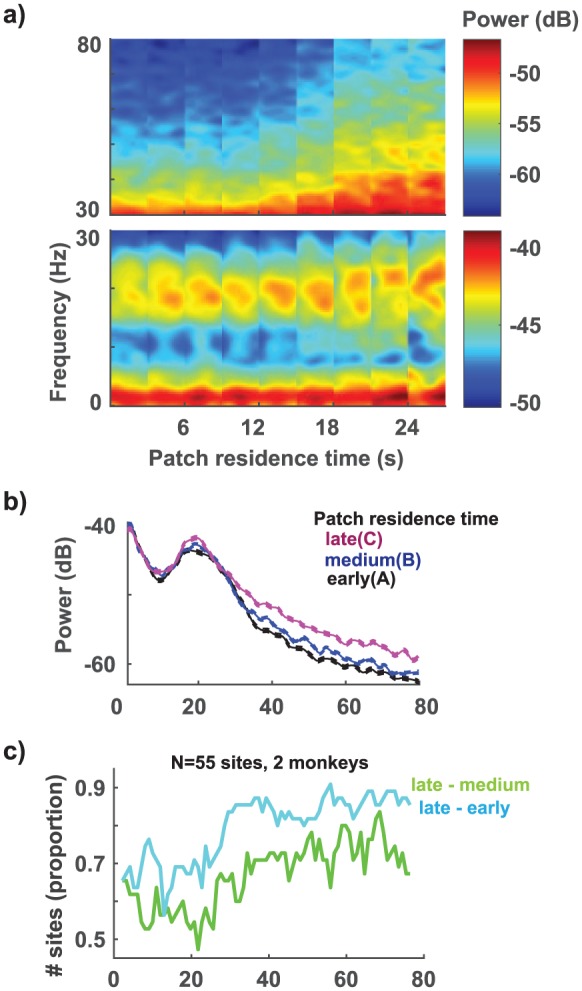
Influence of patch residence time on LFP spectral power. (a) Time–frequency spectrograms showed an increase in the theta (3–9 Hz), beta (13–30 Hz), and gamma (30–80 Hz) band power with patch residence time. Heatmap intensity represents power in decibel. Each tile in the panel represents a 500 ms window at the time of stimulus onset. All the trials in a 3-s patch residence time bin were pooled together to calculate the average spectral power. (b) LFP power spectrum from the example site during a ‘stay’ trial at different patch residence time bins – early (<7.5 s, black), medium (7.5–22.5 s, blue), and late (>22.5 s, magenta). Confidence bands represent s.e.m. (c) When late patch residence times were compared with early patch residence times (cyan trace), as opposed to when late patch residence times were compared with medium patch residence times (green trace), increase in LFP spectral power was observed in significantly more sites.

We next examined modulations in LFP spectral bands that corresponded to changes in travel time. Travel time imposes an opportunity cost and is the major disincentive for abandoning a patch. To test whether LFP spectral bands reflected travel cost, we plotted modulations in spectral power at the time of fixation onset from an example site. Time–frequency spectrum for low frequencies (0–30 Hz; Figure 4(a), lower panel) and higher frequencies (30–80 Hz, Figure 4(a), upper panel) are shown as travel time increases. Interestingly, when trials were segregated into low (<3 s), medium (3–8 s), and high (>8 s) travel time bins, we did not observe significant modulation in spectral power bands, or any other consistent trend, at the example site (Figure 4(b); theta: F(3, 1308) = 2.3, p = 0.081; beta: F(3, 1308) = 0.65, p = 0.578; gamma: F(3, 1308) = 0.67, p = 0.565). Next, we performed a sliding ANOVA and counted the number of sites with a significant increase in LFPs in every 5-Hz frequency bin (Figure 4(c)). LFPs in dACC were modulated by travel time in small proportion of sites (25%–38%, Figure 4(a)). By comparison, LFPs in more than twice as many sites (48%–70% for frequencies < 30 Hz; 66%–89% for frequencies between 30 and 80 Hz, Figure 3(c)) were modulated by patch residence time. Furthermore, when high travel time trials were compared with low travel time trials (Figure 4(c), cyan trace), as opposed to when high travel time trials were compared with medium travel time trials (Figure 3(c), green trace), increase in LFP spectral power was observed in few sites (Figure 4(c), cyan vs green; theta: up to 16%, X²(2, N = 55) = 3.74, p = 0.06; beta: up to 11%, X²(2, N = 55) = 2.85, p = 0.091; gamma: up to 9% (except around 60 Hz), X²(2, N = 55) = 1.94, p = 0.16).

Figure 4.

Influence of travel time on LFP spectral power. (a) Time-frequency spectrograms did not show a significant change in the theta (3–9 Hz), beta (13–30 Hz), and gamma (30–80 Hz) band power with travel time. Heatmap intensity represents power in decibel. Each tile in the panel represents a 500 ms window at the time of stimulus onset. All the trials in a 1.25 s travel time bin were pooled together to calculate the average spectral power. (b) LFP power spectrum from the example site during a ‘stay’ trial at different travel time bins – low (<3 s, black), medium (3–8 s, blue), and high (>8 s, magenta). Confidence bands represent s.e.m. (c) When late patch residence times were compared with early patch residence times (cyan trace), as opposed to when late patch residence times were compared with medium patch residence times (green trace), the number of sites that showed a difference was not significant.

Overall, these observations demonstrate that LFP spectral power in the theta, beta, and gamma bands is robustly influenced by patch residence time, which indicated the value of immediately available reward. LFP spectral bands, were, however, only weakly influenced by travel time, the major cost for abandoning a patch for a new one.

Both travel time and patch residence time modulates neuronal spiking activity

For this analysis, we segregated both patch residence time and travel time into quartiles. Then, we trained a linear classifier (see section ‘Methods’) using a fraction of the data (9 parts out of 10) to classify patch residence time or travel time of the held-out sample. The data consisted of different LFP spectral bands, LFP voltage fluctuations, or neuronal spiking rates. Area under the receiver operating characteristic (AUROC) curve was determined post-classification as a measure of classifier performance. We also randomly shuffled the data prior to classification to obtain a shuffle control.

Consistent with previous results plotted in Figure 3, we observed that LFPs, especially spectral bands corresponding to beta (13–30 Hz) and low gamma band (30–80 Hz), as well as all LFP spectral bands together, encoded patch residence time much better than chance, in a majority of the sites (Figure 5(a); median ± interquartile range (IQR) of the AUROC across 55 sites, 2 monkeys: beta: 0.57 ± 0.04, low gamma: 0.60 ± 0.04, all LFPs: 0.62 ± 0.04). However, these same spectral bands did not encode travel time as well as they encoded patch residence time (Figure 5(b); median ± IQR of the AUROC across 55 sites, 2 monkeys: meta: 0.52 ± 0.03, low gamma: 0.52 ± 0.03, all LFPs: 0.53 ± 0.03). Neuronal firing rates at these same sites, however, encoded both patch residence time (Figure 5(a); median ± IQR of the AUROC across 55 sites, 2 monkeys: spikes: 0.55 ± 0.04) and travel time (Figure 5(b); spikes: 0.56 ± 0.03).

Figure 5.

Encoding of patch residence time and travel time by LFPs and spikes in the dACC. The area under the receiver operating characteristic (AUROC) from a cross-validated linear discriminant analysis to assess how well the ERPs (L-t); LFP power modulations in different spectral bands (D-delta, T-theta, A-alpha, B-beta, Gl-low gamma, Gh-high gamma, L-f – all LFP bands); and changes in the neuronal spiking activity (S) encode the changes in expected reward magnitudes with patch residence time (a) and travel time (b). Consistent with previous analyses, LFP spectral bands especially in the beta, low gamma, or all LFP bands together from many sites (each dot is a site, blue boxes represent 25–75 percentile of AUROC across sites) accounted for changes in patch residence time, significantly better than chance (0.5, dashed horizontal line) and the shuffled control (green boxes; 25–75 percentile). These spectral bands, however, were less informative regarding changes in travel times (b). On the other hand, changes in firing rate of the neurons at many of these sites, encoded changes in patch residence time and travel time, consistent with previous reports (Hayden et al., 2011).

The results from the classification analyses demonstrate that LFP spectral bands at many dACC sites strongly encoded patch residence time but only a few sites weakly encoded the travel time. Neuronal spiking activity at those same sites, however, encoded both patch residence time and travel time.

The primary reason for binning the patch residence time and travel time data was to keep the analyses and the results comparable with a prior study (Hayden et al., 2011). However, to take advantage of the continuous nature of the data, we also carried out a regression-based analysis. The regression models treated the LFP spectral power or the neuronal spiking rate as the dependent variable and the patch residence time and/or travel time as the independent variable(s) (see section ‘Methods’). At an example site (Figures 3–4(a)), we observed that patch residence time was a significant contributor to LFP spectral bands, for example, the low gamma band (coefficient: 0.11 ± 0.04; Tstat: 2.6; degrees of freedom (DOF): 561; p = 0.007), whereas travel time was not (coefficient: –0.01 ± 0.04; Tstat = –0.29; DOF: 561; p = 0.77). On the other hand, both patch residence time (coefficient: 0.1 ± 0.037; Tstat: 2.94; DOF: 572; p = 0.003) and travel time (coefficient: –0.02 ± 0.01; Tstat: –2.4; DOF: 572; p = 0.01) contributed to neuronal spiking rate. Overall, of the 55 sites, for low gamma band, patch residence time was a significant predictor at 12 sites (linear mixed effects model, p < 0.05), whereas travel time was a significant predictor at only 4 sites (linear mixed effects model, p < 0.05). The increase in the number of sites that encoded patch residence time over travel time was significant (4 to 12 sites out of 46; Chi-square Stat = 4.84; p = 0.02). Conversely, for spiking activity, patch residence time and travel time were significant predictors at 17 and 15 sites, respectively (linear mixed effects model, p < 0.05). The number of sites that encoded patch residence time over travel time was not significant (17 to 15 sites out of 46; Chi-square Stat = 0.19; p = 0.66). Table 1 shows the average effect size of patch residence time (top row) and travel time (middle row) on the LFP spectral bands (columns). The bottom row reports the Chi-square statistics and associated p-values (in brackets) based on the increase in the proportion of sites encoding patch residence time over travel time.

Table 1.

The table shows the average effect size of the patch residence time (top row) and travel time (middle row) on the LFP spectral bands (columns).

	Delta	Theta	Alpha	Beta	Low gamma	High gamma	LFP-t	Spike
Residence time	0.06 (12)	0.09 (18)	0.08 (19)	0.04 (19)	0.02 (12)	0.01 (16)	0.16 (13)	0.01 (17)
Travel time	0.001 (5)	0.04 (5)	0.06 (7)	0.02 (9)	0.004 (4)	0.02 (5)	0.003 (4)	0.02 (15)
Chi-square (p-value)	3.53 (0.06)	9.79 (0.001)	7.72 (0.005)	5.13 (0.02)	4.84 (0.02)	7.4 (0.006)	5.84 (0.01)	0.19 (0.66)

The number in brackets indicates the number of sites in which the effect size was significant. The bottom row reports the Chi-square statistics and the associated p-values (in brackets) based on the increase in the proportion of sites encoding patch residence time over travel time.

Again, as observed previously using a linear discriminant analysis, the regression analyses also indicated that at many sites, changes in spectral power in LFPs could be better accounted for by changes in patch residence time than by travel time. By contrast, variation in neuronal spiking activity could be accounted for by changes in both patch residence time and travel time. Converging evidence from the above analyses indicated that LFP spectral bands at many dACC sites strongly encoded patch residence times but only a few sites encoded travel times. At these same recording sites, however, spiking activity signalled both patch residence times and travel times. This mismatch in the information content between LFPs, thought to reflect inputs and local processing, and spikes, thought to reflect outputs of the brain area, constrains the role of the dACC in foraging behaviour.

Spike-field coherence

We observed an increase in spectral power with patch residence time, concomitant with an increase in neuronal firing rate in dACC (Hayden et al., 2011), suggesting that LFP spectral power may mediate the ramping up in firing rates observed during foraging. Furthermore, local oscillations also tend to synchronise neuronal spiking (Buzsáki et al., 2012). That is, an increase in dACC-LFP power may synchronise the activity of more dACC neurons. Spike-field coherence (SFC) provides a way to assess the relationship between changes in spiking activity and changes in spectral power. That is, SFC would be expected to increase when both spiking and field potential power increases.

To understand the changes in SFC with patch residence time, for an example session we binned the data into early, medium, and late residence time bins and the coherence in these bins were plotted separately (Figure 6(a)). SFC in all the bins was greater than chance (dashed horizontal line, Figure 6(a)). Furthermore, SFC increased with patch residence time: SFC for late residence time (magenta, Figure 6(a)) was higher than for medium (blue, Figure 6(a)) and early residence time (black, Figure 6(a)), especially at higher frequencies (>80 Hz). In fact, increase in SFC with patch residence time was significant by regression (p < 0.05, linear mixed effects model) in 12/55 recording sites, especially in high gamma band (80–300 Hz). Increase in SFC with patch residence time was observed in fewer sites and at lower frequencies: 2/55 sites in the delta band, 6/55 sites in theta band, 5/55 sites in alpha, beta, and low gamma band.

Figure 6.

Influence of patch residence time and travel time on spike–LFP coherence. Spike–LFP coherence from an example site binned by patch residence time (a) and travel time (b). Coherence increases with increase in patch residence time and decrease in travel time. Dashed horizontal line at the bottom represents p = 0.05 confidence line. (c) Generalised linear mixed effects models with patch residence time and travel time as fixed effects, respectively, were fit to the spike–LFP coherence data. In general, changes in patch residence time explained the changes in coherence better as indicated by lower Akaike information criteria (AIC). All sites in which the model fit well were used for this plot (see section ‘Results’).

Data were binned into low, medium, and high travel time bins to study the effects of travel time on SFC. In the example session shown in Figure 6(b), SFC decreased with increasing travel time. That is, SFC was higher for low travel time trials (Figure 6(b), black) than for medium travel time trials (Figure 6(b), blue) and high travel time trials (Figure 6(b), magenta). However, significant changes in SFC with travel time were only observed in a few sites: 5/55 sites in delta, theta, and alpha band; 3/55 in beta band; and 4/55 sites in low and high gamma bands. In general, regression models that included patch residence time could account for changes in SFC better than ones that only included travel time (Akaike information criteria (AIC): AIC (patch residence time) – AIC (only travel time) < 0; Figure 6(c)).

Discussion

To determine the optimal time to leave a patch, foragers should track both immediately available reward in the patch and the time costs associated with travelling to a new one. Firing rates of neurons in dACC encode both immediately available reward rate and the long-term average reward rate, which takes into account time costs (Hayden et al., 2011; Kolling et al., 2012, 2016a,b; Wittmann et al., 2016). Whether the time-reward integrated signal observed in dACC neuron firing rates is inherited from other brain areas or arises from local processing remained. By simultaneously monitoring LFPs and spiking outputs from dACC, we observed that LFPs, which have been hypothesised to dominantly reflect inputs and local processing (Buzsáki et al., 2012; Einevoll et al., 2013), were in fact dissimilar to spike rates. LFP spectral bands at a majority of recording sites reflected only immediately available reward whereas spikes at the same sites signalled both reward and time costs. The disjunction between information contained in spiking and LFPs can constrain models of foraging-related processing. These findings endorse a role for dACC in integrating immediate rewards and time costs into a single decision variable – reflective of cost–benefit calculations (Blanchard and Hayden, 2014; Croxson et al., 2009) – central to patch foraging.

ERPs recorded from the scalp and localised to dACC are strongly modulated by the value of received rewards (Emeric et al., 2008; Gehring and Willoughby, 2002). Consistent with these observations, we found significant changes in intracranial LFPs around the time of reward that changed with reward magnitude. Increases in theta and gamma band LFPs in ACC have been observed when stimulus-response mappings change (Womelsdorf et al., 2010). Increases in theta and beta band activity also have been observed in ACC when participants exert cognitive control (Babapoor-Farrokhran et al., 2017). In our study, as within patch reward declined, we observed an increase in theta, beta, and gamma band spectral power. This increase might reflect increasing effort or control needed to override a default stay decision and leave the patch. The increase in spectral power we observed was accompanied by an increase in neuronal firing rates in dACC (Hayden et al., 2011). Increases in theta band power have been shown to be accompanied by increased firing rates of dACC neurons in a phase-locked fashion (Womelsdorf et al., 2010), suggesting LFP spectral power mediates the increase in dACC firing rates during foraging.

Local oscillations in LFP also tend to synchronise local neuronal spiking (Buzsáki et al., 2012). Thus, an increase in LFP power in dACC may increase synchronised firing among dACC neurons. Although, as patch residence time increases, we report an increase in the number of sites showing an increase in spectral power, more conclusive evidence for neuronal synchrony could only come from simultaneous recordings from multiple neurons in dACC as well as LFPs.

Interestingly, LFPs at a few dACC sites reflected time costs. This observation invites the possibility that other unrecorded sites in dACC also may reflect time costs and/or reward modulated by time costs. Furthermore, we selected dACC recording sites based on task-related spiking activity, potentially biasing our LFP results. Future studies that examine dACC spiking activity and field potentials with a multielectrode array spanning different cortical layers may further clarify the role of this brain region.

PCC is reciprocally connected with ACC (Heilbronner and Haber, 2014), receives locus coerulus norepinephrine input (Aston-Jones and Cohen, 2005; Joshi et al., 2016), and is implicated in cognitive control (Botvinick et al., 2004; Hayden et al., 2010; Pearson et al., 2009, 2011). During foraging, travel-time discounted reward signals in dACC could be transmitted to PCC. vmPFC provides a source of information on immediately available reward value for PCC as well (Kolling et al., 2012; McGuire and Kable, 2015; Shenhav et al., 2014; Strait et al., 2014). Foraging decisions require integrating reward and time costs across multiple decisions, a strategic process associated with firing rates in PCC (Barack et al., 2017; Barack and Platt, 2017).

Some recent work has highlighted the possible existence of a hierarchical sequence of processing related to economic choices, which include foraging decisions (Chen and Stuphorn, 2015; Cisek, 2012; Hunt et al., 2012, 2017; Hunt and Hayden, 2017; Strait et al., 2016; Yoo and Hayden, 2018). The proposed hierarchy may begin with orbitofrontal cortex and conclude with motor outputs. Each individual step is small or subtle, but the aggregate effect, along the hierarchy, results in the generation of actions. Our work provides evidence in favour of this viewpoint by providing a rare glimpse of the processes by which two forms of action-relevant information are combined into one.

In summary, foraging requires a core set of computations, which are observed across a wide array of animals (Stephens and Krebs, 1986). The fundamental nature of these computations has placed strong selective pressure on the evolution of cognition and behaviour (DeCasien et al., 2017; González-Forero and Gardner, 2018; Hayden, 2018; Kolling and Akam, 2017; Kolling et al., 2016a,b; Mobbs et al., 2018; Pearson et al., 2014) which in turn has shaped the organisation of the brain (Genovesio et al., 2014; Murray et al., 2017; Passingham and Wise, 2012). These considerations invite the hypothesis that foraging has sculpted the ways that brains make more formal economic decisions, including decision-making under risk and temporal discounting (Bateson and Kacelnik, 1996; Hayden, 2016; Heilbronner, 2017; Kacelnik et al., 2011; Pearson et al., 2010; Santos and Rosati, 2015; Stephens, 2001). According to this line of reasoning, it is not surprising that dACC, which is so central to so many cognitive functions, plays a pivotal role in economic decisions (Ebitz and Hayden, 2016; Kolling et al., 2012, 2016a,b; Shenhav et al., 2013, 2014, 2016). Our findings raise the possibility that local processing within dACC may serve to integrate the value of immediately available rewards and travel time costs, which when combined determine profitability, the core decision variable underlying both foraging and economic decisions.

Methods

Surgical procedures

All procedures were approved by the Duke University Institutional Animal Care and Use Committee and were designed and conducted in compliance with the Public Health Service’s Guide for the Care and Use of Animals.

Behavioural task

The task is described in detail in a previous publication (Hayden et al., 2011). Every trial began with a central fixation spot turning on (‘Fix ON’ in Figure 1). The targets were presented on the screen when the fixation spot turned ON. Following a 500 ms delay, the central fixation square turned off and the monkey was free to select either of the two targets by shifting gaze to it (±2° from the centre of the rectangle). Following choice of either target, the rectangle began to shrink at a constant rate (65 pixels per s) until it disappeared. A reward was then given if the blue ‘stay’ target was chosen and the ITI began (1 s). Because the rate of bar shrinkage was constant, the height of the bar provided an unambiguous cue to the delays associated with the two options on every trial. The delay associated with the blue stay (i.e. remain in patch) rectangle occurred before the reward and was isomorphic to the handling time in foraging decisions (set at 400 ms). The delay associated with the grey ‘switch’ (i.e. leave the patch) rectangle was analogous to the travel time in foraging decisions (ranging from 0.5 to 10.5 s in this experiment). It was set at a random value on each patch, but did not vary in a patch. The fixed delay (inter-trial interval (ITI)) between trials was uncued, but was always the same (1 s). Following the first choice of the blue stay rectangle in each patch, the monkey received 306 µL of water. On subsequent choices of the ‘stay’ target, the reward decreased by 19 µL (although we introduced a small variance in this amount, ε = s.e.m. - standard error of the mean of 1.9 µL). If the monkey continued to choose the blue stay option, its value would eventually reach 0 and remain 0 thereafter. On choosing the grey switch rectangle, the location of the blue and grey rectangles would alternate and the value of the blue rectangle would reset to 306 µL. On choosing the grey rectangle, the size of the grey rectangle and the associated travel time would reset to a new value, chosen from a uniform distribution between 0.5 and 10.5 s.

Horizontal and vertical eye positions were sampled at 1000 Hz by an infrared eye-monitoring camera system (SR Research). Stimuli were controlled by a computer running MATLAB (MathWorks) with Psychtoolbox (Brainard, 1997) and Eyelink Toolbox (Cornelissen et al., 2002). Visual stimuli were small coloured rectangles on a computer monitor placed directly in front of the animal and centred on his eyes. A standard solenoid valve controlled the duration of juice delivery.

Microelectrode recording

Single electrodes (Frederick Haer), lowered using a microdrive (Kopf), were used to record LFPs and spiking activity. Neurons were selected for recording on the basis of the quality of isolation only and not on task-related response properties. We approached ACC through a standard recording grid. ACC was identified by structural magnetic resonance images taken before the experiment (Hayden and Platt, 2010). Neuroimaging was performed at the Center for Advanced Magnetic Development at Duke University Medical Center, on a 3 T MR Imaging Instrument using 1 mm slices. We confirmed that electrodes were in ACC using stereotactic measurements, as well as by listening for characteristic sounds of white and grey matter during recording. Recordings were made between the position of 26 and 30 mm anterior to the interaural plane, with most occurring between 27 and 29. Electrophysiological recordings were made in areas 24c (and possibly 6/32) in the cingulate sulcus, corresponding closely to what is called dorsal anterior cingulate cortex (dACC). The signals were amplified and digitised using a Plexon system (Hayden and Platt, 2010).

Pre-processing LFPs and spikes

Spike and field potential signals were recorded using a Plexon system (2009). The preamplifier box had 16 spike channels (Passband: 150 Hz–8 kHz) and 16 field potential channels (Passband: 0.7 – 300 Hz). Since the field potential signal occupying 0.7–300 Hz was digitised at 1000 Hz, we first low-pass filtered it. The line noise (at 60 Hz) and its harmonics (at 120 and 180 Hz) were modelled using sine waves on small chunks of data (1s windows) and removed from the filtered LFP signal using ‘rmlinesmovingwinc’ from the Chronux toolbox version 2.12 (Bokil et al., 2010). Trials with LFP signals that differed by more than 100 μV between successive sample points (<5% of trials) were removed. Spikes were determined and pre-processed as mentioned in the previous study (Hayden et al., 2011). Spike timestamps were binned using 1 ms bins and then convolved with a Gaussian waveform of σ = 20 ms to obtain a continuous spike density function. The smoothness of the spike density function was determined to match the LFP signal in its overall frequency profile to aid comparison.

Spectrum and spectrogram

Power spectrum analyses were done using Chronux toolbox. LFP spectral power and time-frequency spectrograms were obtained using the multitaper methods available in Chronux toolbox (Thomson, 1982). Spectral power was determined using ‘mtspecgramc’ function. The taper bandwidth was set to 5 Hz, and 1 s of the data was used for analysis. A moving window sampled the next set of data after moving by 10 ms. Spectrograms calculated in this way were normalised by subtracting the log of each value with the log of the baseline power spectrum, in the respective frequency ranges, to get the change in power for each frequency component with respect to time. Power in frequencies ranging from 1.5 through 4 Hz was considered delta band, 3 through 9 Hz was considered theta band, 8 through 13 Hz was considered alpha band, 13 through 30 Hz was considered beta band, 30 through 80 Hz was considered low gamma band, and 80 through 300 Hz was considered high gamma band for all analyses.

Analyses

All the statistical analyses were conducted in MATLAB. Correlations reported are all Pearson’s correlations (default option for ‘corrcoef()’ in MATLAB) unless otherwise mentioned. Data were checked for normality a priori.

ANOVA

One-way ANOVA was performed using ‘Anova1’ comparing LFPs segregated by early, medium, late patch residence times (in Figures 2 and 3), and low, medium, and high travel times (in Figure 4). For the e-LFPs, the average LFP in a 200 ms bin was determined and compared, then the window was moved by 50 ms, and the procedure was repeated. For the spectral data in Figures 3 and 4, average spectral content in a 5 Hz bin was determined and compared, then the window was moved by 1 Hz and the procedure was repeated. ANOVAs were performed for every session separately. Within each session, since the number of trials per bin was variable, trials were resampled with replacement (N = 1000; bootstrap) before performing ANOVA. Resampling ensured the groups that were being compared had equal number of trials and the data distribution was nearly normal. Following ANOVA, post hoc, pairwise comparisons – between bins – were performed using Tukey’s honest significant difference criterion using ‘multcompare’.

Linear discriminant analysis

Each LFP spectral band – delta, theta, alpha, beta, low gamma, high gamma – served as predictors for this analysis (Figure 5(a) and (b); first six bars from the left). ERPs – average time domain LFPs (Figure 5(a) and (b); bar 7), spike density (spikes, Figure 5(a) and (b); bar 8), and finally all spectral bands (LFP-f, all six frequency bands together, Figure 5(a) and (b); bar 8) – were used as predictors to classify patch residence time and travel times. Both patch residence time and travel time were divided into quartiles. The number of samples in each quartile was the same, which ensured that sampling was unbiased for classification. The LFP spectral bands and the spike density data were log-transformed to approximate normal distributions. ERPs were not transformed. Outliers – data beyond 3 standard deviations from the median –were removed prior to classification. Following these pre-processing steps, a fitted discriminant analysis model was obtained using ‘fitcdiscr’. We then performed 10-fold cross-validation using ‘crossval’. Area under the ROC was determined using ‘perfcurve’ for each class against all others (1 vs 2, 3, 4; 2 vs 1, 3, 4; and 3 vs 1, 2, 4). The average ROC was then estimated and shown in Figure 5 (each grey dot). For the shuffle control, the predictors were randomly shuffled before classification. Fifty shuffled classifications were performed and an average across these runs was determined for each site.

Generalised linear model with mixed effects

To understand the relationship between the neural activity (spikes and LFPs) and the patch residence time and travel time, we developed and tested generalised linear models (with mixed effects).

The following models were tested:

1. Activity ~ TT + (1|patch) + (TT – 1|patch)

2. Activity ~ RT + (1|patch)

3. Activity ~ RT + TT + (1|patch) + (TT – 1|patch)

where Activity stands for the spiking activity or LFPs ate a recording site, TT denotes travel time and RT denotes residence time. TT and RT are the fixed effects terms in the models.

Patch is a nominal variable that denoted the patch number. ‘1|patch’ is the random intercept that accounted for baseline differences in activity between patches. ‘TT – 1|patch’ is the random slope term that accounted for differences in activity between patches that was a function of travel time.

Other combinations – including interactions terms for fixed effects, random effects for the residence time, and so on – are not included since those models did not add value when empirically tested. Since the LFP spectral data and smoothened spike rate data were right skewed and all-positive, they were modelled using a ‘Gamma’ distribution with a ‘reciprocal’ link function. All analyses were carried out in MATLAB using the ‘fitglme’ function.

SFC

Spike data was binned into 100 ms bins to match the sampling rate of the field potential data. Spectral power was determined for the field potential data. Then, SFC was computed using the ‘coherencycpb’ function in the Chronux toolbox. To test whether coherence changed with residence time or travel time, a generalised linear models were developed. The models were similar to the ones utilized to understand the influence of residence time and travel time on the field potential and spiking activity.

The following models were tested:

1. Coherence ~ TT + (1|patch) + (TT – 1|patch)

2. Coherence ~ RT + (1|patch)

3. Coherence ~ RT + TT + (1|patch) + (TT – 1|patch)

where TT denotes travel time and RT denotes residence time. TT and RT are the fixed effects terms in the models.

Patch is a nominal variable that denoted the patch number. ‘1|patch’ is the random intercept that accounted for baseline differences in activity between patches. ‘TT – 1|patch’ is the random slope term that accounted for differences in activity between patches that was a function of travel time.

Coherence computed using the above models is shown in Figure 6. Akaike information criteria (AIC) was calculated for each of the models. AIC was determined by computing [2 log L + kp], where L is the likelihood function, p is the number of parameters in the model, and k is 2. A lower AIC means a model is considered to be closer to the truth.

References

- Anderson DE, Vogel EK, Awh E. (2013) A common discrete resource for visual working memory and visual search. Psychological Science 24(6): 929–938. [DOI] [PMC free article] [PubMed] [Google Scholar] [Retracted]
- Aston-Jones G, Cohen JD. (2005) An integrative theory of locus coeruleus-norepinephrine function: Adaptive gain and optimal performance. Annual Review of Neuroscience 28(1): 403–450. [DOI] [PubMed] [Google Scholar]
- Babapoor-Farrokhran S, Vinck M, Womelsdorf T, et al. (2017) Theta and beta synchrony coordinate frontal eye fields and anterior cingulate cortex during sensorimotor mapping. Nature Communications 8(2): 13967. [DOI] [PMC free article] [PubMed] [Google Scholar]
- Barack DL, Platt ML. (2017) Engaging and Exploring: Cortical Circuits for Adaptive Foraging Decisions. In: Stevens J. (ed) Impulsivity. Nebraska Symposium on Motivation, vol 64 Springer, Cham. [PubMed] [Google Scholar]
- Barack DL, Chang SWC, Platt ML. (2017) Posterior cingulate neurons dynamically signal decisions to disengage during foraging. Neuron 96(2): 339–347. e5. [DOI] [PMC free article] [PubMed] [Google Scholar]
- Bateson M, Kacelnik A. (1996) Rate currencies and the foraging starling: The fallacy of the average revisited. Behavioral Ecology 7(3): 341–352. [Google Scholar]
- Björklund A, Dunnett SB. (2007) Dopamine neuron systems in the brain: An update. Trends in Neurosciences 30(5): 194–202. [DOI] [PubMed] [Google Scholar]
- Blanchard TC, Hayden BY. (2014) Neurons in dorsal anterior cingulate cortex signal postdecisional variables in a foraging task. Journal of Neuroscience 34(2): 646–655. [DOI] [PMC free article] [PubMed] [Google Scholar]
- Blanchard TC, Hayden BY. (2015) Monkeys are more patient in a foraging task than in a standard intertemporal choice task. PLoS ONE 10(2): e0117057. [DOI] [PMC free article] [PubMed] [Google Scholar]
- Blanchard TC, Strait CE, Hayden BY. (2015) Ramping ensemble activity in dorsal anterior cingulate neurons during persistent commitment to a decision. Journal of Neurophysiology 114(4): 2439–2449. [DOI] [PMC free article] [PubMed] [Google Scholar]
- Bokil H, Andrews P, Kulkarni JE, et al. (2010) Chronux: A platform for analyzing neural signals. Journal of Neuroscience Methods 192(1): 146–151. [DOI] [PMC free article] [PubMed] [Google Scholar]
- Botvinick MM, Cohen JD, Carter CS. (2004) Conflict monitoring and anterior cingulate cortex: An update. Trends in Cognitive Sciences 8(12): 539–546. [DOI] [PubMed] [Google Scholar]
- Brainard DH. (1997) The psychophysics toolbox. Spatial Vision 10(4): 433–436. [PubMed] [Google Scholar]
- Buzsáki G, Anastassiou CA, Koch C. (2012) The origin of extracellular fields and currents-EEG, ECoG, LFP and spikes. Nature Reviews Neuroscience 13(6): 407–420. [DOI] [PMC free article] [PubMed] [Google Scholar]
- Cain MS, Vul E, Clark K, et al. (2012) A Bayesian optimal foraging model of human visual search. Psychological Science 23(9): 1047–1054. [DOI] [PubMed] [Google Scholar]
- Charnov EL. (1976) Optimal foraging, the marginal value theorem. Theoretical Population Biology 9(2): 129–136. [DOI] [PubMed] [Google Scholar]
- Chen X, Stuphorn V. (2015) Sequential selection of economic good and action in medial frontal cortex of macaques during value-based decisions. Elife 4(11): e09418. [DOI] [PMC free article] [PubMed] [Google Scholar]
- Cisek P. (2012) Making decisions through a distributed consensus. Current Opinion in Neurobiology 22(6): 927–936. [DOI] [PubMed] [Google Scholar]
- Cornelissen FW, Peters EM, Palmer J. (2002) The eyelink toolbox: Eye tracking with MATLAB and the psychophysics toolbox. Behavior Research Methods, Instruments, & Computers 34(4): 613–617. [DOI] [PubMed] [Google Scholar]
- Croxson PL, Walton ME, Reilly JXO, et al. (2009) Effort-based cost–benefit valuation and the human brain. Brain 29(14): 4531–4541. [DOI] [PMC free article] [PubMed] [Google Scholar]
- Daw ND, O’Doherty JP, Dayan P, et al. (2006) Cortical substrates for exploratory decisions in humans. Nature 441(7095): 876–879. [DOI] [PMC free article] [PubMed] [Google Scholar]
- DeCasien AR, Williams SA, Higham JP. (2017) Primate brain size is predicted by diet but not sociality. Nature Ecology and Evolution 1(5): 0112. [DOI] [PubMed] [Google Scholar]
- Dukas R. (2002) Behavioural and ecological consequences of limited attention. Philosophical Transactions of the Royal Society B 357(1427): 1539–1547. [DOI] [PMC free article] [PubMed] [Google Scholar]
- Ebitz RB, Hayden BY. (2016) Dorsal anterior cingulate: A Rorschach test for cognitive neuroscience. Nature Neuroscience 19(10): 1278–1279. [DOI] [PubMed] [Google Scholar]
- Einevoll GT, Kayser C, Logothetis NK, et al. (2013) Modelling and analysis of local field potentials for studying the function of cortical circuits. Nature Reviews Neuroscience 14(11): 770–785. [DOI] [PubMed] [Google Scholar]
- Emeric EE, Brown JW, Leslie M, et al. (2008) Performance monitoring local field potentials in the medial frontal cortex of primates: Anterior cingulate cortex. Journal of Neurophysiology 99(2): 759–772. [DOI] [PMC free article] [PubMed] [Google Scholar]
- Fu W-T, Pirolli P. (2007) SNIF-ACT: A cognitive model of user navigation on the world wide web. Human-Computer Interaction 22(4): 355–412. [Google Scholar]
- Gehring WJ, Willoughby AR. (2002) The medial frontal cortex and the rapid processing of monetary gains and losses. Science 295(5563): 2279–2282. [DOI] [PubMed] [Google Scholar]
- Genovesio A, Wise SP, Passingham RE. (2014) Prefrontal-parietal function: From foraging to foresight. Trends in Cognitive Sciences 18(2): 72–81. [DOI] [PubMed] [Google Scholar]
- González-Forero M, Gardner A. (2018) Inference of ecological and social drivers of human brain-size evolution. Nature 557(7706): 554–557. [DOI] [PubMed] [Google Scholar]
- Hayden BY. (2016) Time discounting and time preference in animals: A critical review. Psychonomic Bulletin & Review 23(1): 39–53. [DOI] [PubMed] [Google Scholar]
- Hayden BY. (2018) Economic choice: The foraging perspective. Current Opinion in Behavioral Sciences 24(12): 1–6. [Google Scholar]
- Hayden BY, Pearson JM, Platt ML. (2011) Neuronal basis of sequential foraging decisions in a patchy environment. Nature Neuroscience 14(7): 933–939. [DOI] [PMC free article] [PubMed] [Google Scholar]
- Hayden BY, Platt ML. (2010) Neurons in Anterior Cingulate Cortex Multiplex Information about Reward and Action. Journal of Neuroscience 30(9): 3339–3346. [DOI] [PMC free article] [PubMed] [Google Scholar]
- Hayden BY, Smith DV, Platt ML. (2010) Cognitive control signals in posterior cingulate cortex. Frontiers in Human Neuroscience 4(12): 223. [DOI] [PMC free article] [PubMed] [Google Scholar]
- Heilbronner SR. (2017) Modeling risky decision-making in nonhuman animals: Shared core features. Current Opinion in Behavioral Sciences 16(8): 23–29. [DOI] [PMC free article] [PubMed] [Google Scholar]
- Heilbronner SR, Haber SN. (2014) Frontal cortical and subcortical projections provide a basis for segmenting the cingulum bundle: Implications for neuroimaging and psychiatric disorders. Journal of Neuroscience 34(30): 10041–10054. [DOI] [PMC free article] [PubMed] [Google Scholar]
- Heilbronner SR, Hayden BY. (2016) Dorsal anterior cingulate cortex: A bottom-up view. Annual Review of Neuroscience 39(1): 149–170. [DOI] [PMC free article] [PubMed] [Google Scholar]
- Hills TT, Pachur T. (2012) Dynamic search and working memory in social recall. Journal of Experimental Psychology: Learning, Memory, and Cognition 38(1): 218–228. [DOI] [PubMed] [Google Scholar]
- Hills TT, Jones MN, Todd PM. (2012) Optimal foraging in semantic memory. Psychological Review 119(2): 431–440. [DOI] [PubMed] [Google Scholar]
- Hills TT, Todd PM, Goldstone RL. (2010) The central executive as a search process: Priming exploration and exploitation across domains. Journal of Experimental Psychology: General 139(4): 590–609. [DOI] [PMC free article] [PubMed] [Google Scholar]
- Hills TT, Todd PM, Jones MN. (2015) Foraging in semantic fields: How we search through memory. Topics in Cognitive Science 7(3): 513–534. [DOI] [PubMed] [Google Scholar]
- Hunt LT, Hayden BY. (2017) A distributed, hierarchical and recurrent framework for reward-based choice. Nature Reviews Neuroscience 18(3): 172–182. [DOI] [PMC free article] [PubMed] [Google Scholar]
- Hunt LT, Kolling N, Soltani A, et al. (2012) Mechanisms underlying cortical activity during value-guided choice. Nature Neuroscience 15(3): 470–476. [DOI] [PMC free article] [PubMed] [Google Scholar]
- Hunt LT, Malalasekera W, de Berker A, et al. (2017) Triple dissociation of attention and decision computations across prefrontal cortex. Nature Neuroscience 21(9): 1471–1481. [DOI] [PMC free article] [PubMed] [Google Scholar]
- Joshi S, Li Y, Kalwani RM, et al. (2016) Relationships between pupil diameter and neuronal activity in the locus coeruleus, colliculi, and cingulate cortex. Neuron 89(1): 221–234. [DOI] [PMC free article] [PubMed] [Google Scholar]
- Kacelnik A, Vasconcelos M, Monteiro T, et al. (2011) Darwin’s ‘tug-of-war’ vs. starlings’ ‘horse-racing’: How adaptations for sequential encounters drive simultaneous choice. Behavioral Ecology and Sociobiology 65(3): 547–558. [Google Scholar]
- Kolling N, Akam T. (2017) (Reinforcement?) Learning to forage optimally. Current Opinion in Neurobiology 46(10): 162–169. [DOI] [PubMed] [Google Scholar]
- Kolling N, Behrens TEJ, Mars RB, et al. (2012) Neural mechanisms of foraging. Science 335(6077): 95–98. [DOI] [PMC free article] [PubMed] [Google Scholar]
- Kolling N, Behrens TEJ, Wittmann MK, et al. (2016. a) Multiple signals in anterior cingulate cortex. Current Opinion in Neurobiology 37: 36–43. [DOI] [PMC free article] [PubMed] [Google Scholar]
- Kolling N, Wittmann MK, Behrens TEJ, et al. (2016. b) Value, search, persistence and model updating in anterior cingulate cortex. Nature Neuroscience 19(10): 1280–1285. [DOI] [PMC free article] [PubMed] [Google Scholar]
- McGuire JT, Kable JW. (2015) Medial prefrontal cortical activity reflects dynamic re-evaluation during voluntary persistence. Nature Neuroscience 18(5): 760–766. [DOI] [PMC free article] [PubMed] [Google Scholar]
- Milton K. (1988) Foraging behaviour and the evolution of primate intelligence. In: Byrne RW, Whiten A. (eds) Machiavellian Intelligence: Social Expertise and the Evolution of Intellect in Monkeys Apes and Humans. New York, NY: Clarendon Press/Oxford University Press, pp. 285–305. [Google Scholar]
- Mitzdorf U. (1985) Current source-density method and application in cat cerebral cortex: Investigation of evoked potentials and EEG phenomena. Physiological Reviews 65(1): 37–100. [DOI] [PubMed] [Google Scholar]
- Mobbs D, Trimmer PC, Blumstein DT, et al. (2018) Foraging for foundations in decision neuroscience: Insights from ethology. Nature Reviews Neuroscience 19(5): 419–427. [DOI] [PMC free article] [PubMed] [Google Scholar]
- Monosov IE, Trageser JC, Thompson KG. (2008) Measurements of simultaneously recorded spiking activity and local field potentials suggest that spatial selection emerges in the frontal eye field. Neuron 57(4): 614–625. [DOI] [PMC free article] [PubMed] [Google Scholar]
- Murray EA, Wise SP, Graham KS. (2017) Representational specializations of the hippocampus in phylogenetic perspective. Neuroscience Letters 680(7): 4–12. [DOI] [PMC free article] [PubMed] [Google Scholar]
- Newell A. (1992) Précis of unified theories of cognition. Behavioral and Brain Sciences 15(3): 425–437. [DOI] [PubMed] [Google Scholar]
- Passingham RE, Wise SP. (2012) Caudal prefrontal cortex. In: The Neurobiology of the Prefrontal Cortex, Oxford: Oxford University Press, pp. 132–156. [Google Scholar]
- Payne SJ, Duggan GB. (2011) Giving up problem solving. Memory and Cognition 39(5): 902–913. [DOI] [PubMed] [Google Scholar]
- Pearson JM, Hayden BY, Platt ML. (2010) Explicit information reduces discounting behavior in monkeys. Frontiers in Psychology 1(12): 237. [DOI] [PMC free article] [PubMed] [Google Scholar]
- Pearson JM, Hayden BY, Raghavachari S, et al. (2009) Neurons in posterior cingulate cortex signal exploratory decisions in a dynamic multioption choice task. Current Biology 19(18): 1532–1537. [DOI] [PMC free article] [PubMed] [Google Scholar]
- Pearson JM, Heilbronner SR, Barack DL, et al. (2011) Posterior cingulate cortex: Adapting behavior to a changing world. Trends in Cognitive Sciences 15(4): 143–151. [DOI] [PMC free article] [PubMed] [Google Scholar]
- Pearson JM, Watson KK, Platt ML. (2014) Decision making: The neuroethological turn. Neuron 82(5): 950–965. [DOI] [PMC free article] [PubMed] [Google Scholar]
- Pirolli P. (2007) Information foraging theory: Adaptive interaction with information. In: Information Foraging Theory. New York, NY: Oxford University Press, Inc. [Google Scholar]
- Santos L, Rosati A. (2015) The evolutionary roots of human decision making. Annual Review of Psychology 66(1): 321–347. [DOI] [PMC free article] [PubMed] [Google Scholar]
- Sendhilnathan N, Basu D, Murthy A. (2017) Simultaneous analysis of the LFP and spiking activity reveals essential components of a visuomotor transformation in the frontal eye field. Proceedings of the National Academy of Sciences of the United States of America 114(24): 6370–6375. [DOI] [PMC free article] [PubMed] [Google Scholar]
- Shenhav A, Botvinick MM, Cohen JD. (2013) Review the expected value of control: An integrative theory of anterior cingulate cortex function. Neuron 79(2): 217–240. [DOI] [PMC free article] [PubMed] [Google Scholar]
- Shenhav A, Straccia MA, Botvinick MM, et al. (2016) Dorsal anterior cingulate and ventromedial prefrontal cortex have inverse roles in both foraging and economic choice. Cognitive, Affective, & Behavioral Neuroscience 16(6): 1127–1139. [DOI] [PubMed] [Google Scholar]
- Shenhav A, Straccia MA, Cohen JD, et al. (2014) Anterior cingulate engagement in a foraging context reflects choice difficulty, not foraging value. Nature Neuroscience 17(9): 1249–1254. [DOI] [PMC free article] [PubMed] [Google Scholar]
- Stephens DW. (2001) The adaptive value of preference for immediacy: When shortsighted rules have farsighted consequences. Behavioral Ecology 12(3): 330–339. [Google Scholar]
- Stephens DW, Krebs JR. (1986) Foraging theory. In: Evolutionary Behavioral Ecology. Princeton: Princeton University Press. [Google Scholar]
- Strait CE, Blanchard TC, Hayden BY. (2014) Reward value comparison via mutual inhibition in ventromedial prefrontal cortex. Neuron 82(6): 1357–1366. [DOI] [PMC free article] [PubMed] [Google Scholar]
- Strait CE, Sleezer BJ, Blanchard TC, et al. (2016) Neuronal selectivity for spatial positions of offers and choices in five reward regions. Journal of Neurophysiology 115(3): 1098–1111. [DOI] [PMC free article] [PubMed] [Google Scholar]
- Thomson DJ. (1982) Spectrum estimation and harmonic analysis. Proceedings of the IEEE 70(9): 1055–1096. [Google Scholar]
- Vogt BA, Rosene DL, Pandya DN. (1979) Thalamic and cortical afferents differentiate anterior from posterior cingulate cortex in the monkey. Science 204(4389): 205–207. [DOI] [PubMed] [Google Scholar]
- Williams SM, Goldman-Rakic PS. (1993) Characterization of the dopaminergic innervation of the primate frontal cortex using a dopamine-specific antibody. Cerebral Cortex 3(3): 199–222. [DOI] [PubMed] [Google Scholar]
- Wittmann MK, Kolling N, Akaishi R, et al. (2016) Predictive decision making driven by multiple time-linked reward representations in the anterior cingulate cortex. Nature Communications 7(1): 12327. [DOI] [PMC free article] [PubMed] [Google Scholar]
- Wolfe JM. (2018) When is it time to move to the next raspberry bush? Foraging rules in human visual search. Journal of Vision 13(3): 10. [DOI] [PMC free article] [PubMed] [Google Scholar]
- Womelsdorf T, Johnston K, Vinck M, et al. (2010) Theta-activity in anterior cingulate cortex predicts task rules and their adjustments following errors. Proceedings of the National Academy of Sciences of the United States of America 107(11): 5248–5253. [DOI] [PMC free article] [PubMed] [Google Scholar]
- Yoo SBM, Hayden BY. (2018) Economic choice as an untangling of options into actions. Neuron 99(3): 434–447. [DOI] [PMC free article] [PubMed] [Google Scholar]