Vent Pipe Emissions from Storage Tanks at Gas Stations: Implications for Setback Distances

Abstract

At gas stations, fuel vapors are released into the atmosphere from storage tanks through vent pipes. Little is known about when releases occur, their magnitude, and their potential health consequences. Our goals were to quantify vent pipe releases and examine exceedance of short-term exposure limits to benzene around gas stations. At two US gas stations, we measured volumetric vent pipe flow rates and pressure in the storage tank headspace at high temporal resolution for approximately three weeks. Based on the measured vent emission and meteorological data, we performed air dispersion modeling to obtain hourly atmospheric benzene levels. For the two gas stations, average vent emission factors were 0.17 and 0.21 kg of gasoline per 1,000 L dispensed. Modeling suggests that at one gas station, a 1-hour Reference Exposure Level (REL) for benzene for the general population (8 ppb) was exceeded only closer than 50 m from the station’s center. At the other gas station, the REL was exceeded on two different days and up to 160 m from the center, likely due to non-compliant bulk fuel deliveries. A minimum risk level for intermediate duration (>14–364 days) benzene exposure (6 ppb) was exceeded at the elevation of the vent pipe opening up to 7 and 8 m from the two gas stations. Recorded vent emission factors were more than 10 times higher than estimates used to derive setback distances for gas stations. Setback distances should be revisited to address temporal variability and pollution controls in vent emissions.

1. INTRODUCTION

In the US, approximately 143 billion gal (541 billion L) of gasoline were dispensed in 2016 at gas stations¹ resulting in release of unburned fuel to the environment in the form of vapor or liquid.² This is a public health concern, as unburned fuel chemicals such as benzene, toluene, ethyl-benzene, and xylenes (BTEX) are harmful to humans.³ Benzene is of special concern because it is causally associated with different types of cancer.⁴ Truck drivers delivering gasoline and workers dispensing fuel have among the highest exposures to fuel releases.⁴ However, people living near or working in retail at gas stations, and children in schools and on playgrounds can also be exposed, with distance to the gas stations significantly affecting exposure levels.^5–8 A meta-analysis⁹ of three case-control studies^10–12 suggests that childhood leukemia is associated with residential proximity to gas stations.

Sources of unburned fuel releases at gas stations include leaks from storage tanks, accidental spills from the nozzles of gas dispensers,^13–15 fugitive vapor emissions through leaky pipes and fittings, vehicle tank vapor releases when refueling, and leaky hoses, all of which can contribute to subsurface and air pollution.² Routine fuel releases also occur through vent pipes of fuel storage tanks but are less noticeable because the pipes are typically tall, e.g., 4 m. These vent pipes are put in place to equilibrate pressures in the tanks and can be located as close as a few meters from residential buildings in dense urban settings (Figure 1).

Figure 1:

The three vent pipes (enclosed by the red ellipse) on the right side of the convenience store of a gas station are less than 10 m away from the residential building.

Unburned fuel can be released from storage tanks into the environment through “working” and “breathing” losses.¹⁶ A working loss occurs when liquid is pumped into or out of a tank. For a storage tank, this can happen when it is refilled from a tanker truck or when fuel is dispensed to refuel vehicles¹⁷ if the pressure in the storage tank exceeds the relief pressure of the pressure/vacuum (P/V) valve.¹⁸ P/V valve threshold pressures are typically set to around +3 and −8 inches of water column (iwc) (7.5 and −20 hPa). However, P/V valves are not always used, particularly in cold climates, as valves may fail under cold weather conditions.¹⁷

Breathing losses occur when no liquid is pumped into or out of a tank because of vapor expansion and contraction due to temperature and barometric pressure changes or because pressure in the storage tank may increase when fuel in the tank evaporates.^16,18 Although delayed or redirected by the P/V valve, breathing emissions can be significant and represent an environmental and health concern.¹⁶

Stage I vapor recovery systems, put in place to prevent working losses while delivering fuel to a station, collect the vapors displaced while loading a storage tank, redirecting them into the delivery truck. Stage II vapor recovery systems minimize working losses while delivering gas from the storage tank to the customer’s car. During Stage II vapor recovery, gasoline vapors can be released through the vent pipe, if the sum of the flow rates of the returned volume and of the fuel evaporating within the storage tank is greater than the volume of liquid gasoline dispensed.¹⁷ We refer to this scenario as pressure while dispensing (PWD). In theory, a properly designed Stage II vapor recovery system should not have working losses, although in practice this is not typically the case.¹⁹

Regulations on setback distances for gas stations are based on lifetime cancer risk estimates. Several studies have assessed benzene cancer risk near gas stations.^20–25 Based on cancer risk estimations, the California Air Resources Board (CARB) recommended that schools, day cares, and other sensitive land uses should not be located within 300 ft (91 m) of a large gas station (defined as a facility with an annual sales volume of 3.6 million gallons = 13.6 million L or greater).²⁶ This CARB recommendation has not been adopted by all US states, and within states setback distances can depend on local government. Notably, CARB regulations do not account for short term exposure limits and health effects. An important limitation of existing regulations is the use of average gasoline emission rates estimated in the 90’s that do not consider excursions.²⁷

The main objective of this study is to evaluate fuel vapor releases through vent pipes of storage tanks at gas stations based on vent emission measurements conducted at two gas stations in the US in 2009 and 2015, including the characterization of excursions at a high temporal resolution (~minutes) and meteorological conditions at an hourly temporal resolution. In addition, we performed hourly simulations of atmospheric transport of emitted fuel vapors to inform regulations on setback distances between gas stations and adjacent sensitive land uses by comparing modeled benzene concentrations to four 60-min benzene exposure limits: an acute Reference Exposure Level (REL) for infrequent (once per month or less) exposure²⁸ and Emergency Response Planning Guidelines ERPG-1, ERPG-2 and ERPG-3.²⁹ Finally we compared simulated benzene levels to a Minimal Risk Level (MRL) for benzene for intermediate exposure duration (14 to 364 days)³⁰ because that duration window includes our duration of data collection. See Table 1 for the various benzene exposure limits and issuing agencies.

Table 1:

Benzene exposure limits, to which we compared simulation results. For unit conversion, we assumed a temperature of 25°C, i.e., 1 ppm = 3,194 μg/m³.²⁷

Agency	Name	Value (ppb)	Value (μg/m³)	Exposure duration
California Office of Environmental Health Hazard Assessment (OEHHA)	REL	8	26	1 hour
American Industrial Hygiene Association (AIHA)	ERPG-1	50	159,700	1 hour
AIHA	ERPG-2	150	479,100	1 hour
AIHA	ERPG-3	1,000	3,194,000	1 hour
Agency for Toxic Substances and Disease Registry (ATSDR)	MRL	6	19	14 to 364 days

ERPG = Emergency Response Planning Guidelines. The primary focus of ERPGs is to provide guidelines for short-term exposures to airborne concentrations of acutely toxic, high-priority chemicals.

2. METHODS

Although we provide SI unit conversions, we report some measures in English engineering units (ft, gal, and lb) as regulatory agencies such as CARB use these units.

2.1. Sites

Data for this study were obtained from vent release measurements conducted at two gas stations as part of technical assistance to the gas stations to quantify fuel vapor losses through the vent pipes of their storage tanks. A motivation for conducting the measurements was to perform a cost-benefit analysis to compare the economic losses due to the lost fuel versus the cost of technologies that reduce the emissions. The exact location of the two gas stations is not revealed for confidentiality reasons. The gas station managers and staff who authorized the collection and analysis of these data have not been involved in the current manuscript.

The first gas station, “GS-MW,” was located in the US Midwest and is a 24-hour operation. The study was conducted from December 2014 to January 2015 for 20 full days, and fuel sales ${\dot{V}}_{\mathit{\text{sales}}}$ were about 450,000 gal (1.7 million L) per month. Fuel deliveries to the gas station usually took place during the nighttime. The second gas station, “GS-NW,” was located on the US Northwest coast and closed at night. Hours of operation were between 6:00 am and 9:30 pm on weekdays and between 7 am and 7 pm on weekends. That study was conducted in October 2009 for 18 full days, and fuel sales were ${\dot{V}}_{\mathit{\text{sales}}}$ ~700,000 gal (2.6 million L) per month.

Both gas stations are considered to be high-volume, because they dispense more than 3.6 million gallons of gasoline (both regular and premium) per year,²⁶ and fuel was stored in underground storage tanks (USTs), which is typical in the US. Both gas stations had Stage II vapor recovery installed using the vacuum-assist method. In that method, gasoline vapors, which would be ejected into the atmosphere as a working loss during refueling of customer vehicle tanks, are collected at the vehicle/nozzle interface by a vacuum pump. The recovered vapors are then directed via a coaxial hose back into the combined storage tank ullage (head space) of the gas station. Stage I vapor recovery was also used at both gas stations during fuel deliveries. Both sites had a 3-inch diameter (7.5 cm) single above-grade vent pipe with below-grade manifold that connected the vent lines from several USTs; the cracking pressures of the P/V valves were set to +3 and −8 iwc (+7.5 and −20 hPa).

2.2. Vent Emission Measurements

To quantify evaporative fuel releases through the vent pipe of a storage tank, the volumetric flow of the mixture of gasoline vapor and air was measured in the vent pipe. A dry gas diaphragm flow meter (American Meter Company, Model AC-250) was used. For each cubic foot (28 L) of gas flowing through the meter, a digital pulse was generated. Every minute, the number of pulses was read out and stored together with date and time on a data logger. Gas flow meters were obtained from a distributor calibrated and equipped with temperature compensation and a pulse meter.

To determine the time-dependent volumetric flow rate Q(t) of the gasoline vapor/air mixture through the vent pipe, the time series of measured flow volumes were integrated over an averaging period (15 or 60 minutes) and divided by the duration of that period. I.e., Q(t) is given by the number of pulses registered by the gas flow meter in a time window multiplied by 1 cubic foot and divided by the averaging time. The 15-minute averaging time was chosen to visualize time-dependent data, while the 60-minute averaging time was chosen because air pollution simulations were performed at that resolution.

Gas pressure p in the ullage of the storage tank was measured to assess vent emission patterns. For instance, releases can occur when the pressure exceeds the cracking pressure of the P/V valve in the vent pipe (the dry gas flow meter was fitted with a P/V valve on the outlet). Pressure was measured with a differential pressure sensor (Cerabar PMC 41, Endress+Hauser) every 4 seconds, and 2-minute average values were stored. The sensor range was scaled from −15 to +15 iwc (−37 to +37 hPa), with a full scale accuracy of 0.20%. We also obtained 15- and 60-minute averaged tank pressure data p(t) where averages represent the means of the 2-minute average pressure measurements taken during each time window.

2.3. Descriptive Analysis

For the 60-minute flow rate, we calculated medians and inter quartile ranges (IQRs). To illustrate diurnal fluctuations in vapor emissions, we created box plots for the 60-minute flow rate distribution that occurred during each hour of the day. Spearman correlation coefficients between the time series for pressure and flow rate were calculated to evaluate whether pressure can be used to infer vent emissions.

To estimate the mass flow rate of gasoline ${\dot{m}}_{gas}$ that is released through the vent pipe in the form of a mixture of gasoline vapors and fresh air, we assumed, following the protocol of a study by the California Air Pollution Control Officers Association (CAPCOA) that assessed risks from fuel emissions from gas station (Appendix D-2²⁷), that the density of gasoline vapors in this mixture is given by ${\rho }_{gas}^{(v)}=$ 0.3 × 65 lb / 379 ft³ = 0.824 kg/m³, i.e., the molar percentages of gasoline and air were 30% and 70%, respectively. Then the volumetric flow rate Q can be converted into a mass flow rate of the vaporized gasoline:

$${\dot{m}}_{gas}={\rho }_{gas}^{(v)}Q$$ (Eq. 1)

To arrive at vent emission factors, we first calculated the mean volumetric flow rate $\overline{Q}$, and then the mean mass flow rate ${\overline{\dot{m}}}_{gas}={\rho }_{gas}^{(v)}\overline{Q}$. From the latter, one can calculate the vent emission factor

$${\text{EF}}_{\mathit{\text{vent}}}={\overline{\dot{m}}}_{gas}/{\dot{V}}_{\text{sales}}$$ (Eq. 2)

For ${\text{EF}}_{\mathit{\text{vent}}}$, CARB uses units of pounds of emitted gasoline vapors (also called total organic gases (TOG)) per 1,000 gallons dispensed, or more briefly lb/kgal where kgal stands for kilogallons.

As we were not able to measure benzene levels in the tank ullage, we assumed like the CAPCOA study (Section C) that the density of the mixture of gasoline vapors and fresh air was ${\rho }_{mix}^{(v)}=$ 1.05 lb/ft³ = 1.682 kg/m³ and that the emitted gasoline vapor/air mixture contained 0.3% of benzene by weight.²⁷ Therefore, the mass flow rate of benzene through the vent pipe was estimated as follows:

$${\dot{m}}_{\mathit{\text{benz}}}=0.003{\rho }_{mix}^{(v)}Q$$ (Eq. 3)

2.4. Air Pollution Modeling

We used the AERMOD Modeling System developed by the US Environmental Protection Agency (EPA) to model the dispersion of benzene vapors released into the environment through vent pipes of fuel storage tanks and from other sources.³¹ AERMOD simulates atmospheric pollutant transport at a 1-hour temporal resolution. 3D polar grids were created with the gas station in the origin and potential receptors at different radial distances (up to 170 meters) and angles (10° increments). The grids were placed at the ground level (z = 0 m), in the breathing zone (z = 2 m), and at the 2^nd floor level (z = 4 m) where the vent pipe emissions were assumed to occur. The topography was simplified for modeling purposes consistent with the CAPCOA study,²⁷ i.e., the terrain was assumed to be flat with no buildings present. Vent pipe emissions were modeled as a capped point source. Chemical reactions of benzene were not modeled, as residence times of atmospheric benzene are on the order of hours or even days,³² i.e. much longer than the travel time of benzene vapors across the 340-m diameter model domain.

For the period of time when vent emission measurements were made, we obtained meteorological data at a 1-hour temporal resolution that are representative for the geographic locations of the two gas stations. Table SI-1 provides descriptive statistics of that data. The time series were used in AERMOD to model the transport of benzene in the temporally varying turbulent atmosphere. We also used the 1-hour average time series of benzene emission rates (Eq. 3) as an input into AERMOD.

To evaluate at each grid point whether OEHHA’s acute REL or AIHA’s ERPG levels were exceeded at least once, we determined maximum 1-hour average benzene concentrations that were simulated for about three weeks. To evaluate how often the OEHHA REL was exceeded at each grid point in the breathing zone, we created plots indicating the number of exceedances and the day when the maximum benzene level was observed.

To facilitate comparison to published benzene measurements around gas stations, we determined for each simulated radial distance from a gas station the mean of the average concentrations simulated for each ten degree increment on the radius around the gas station.

3. RESULTS: VENT RELEASES

3.1. Times Series of Tank Pressure and Flow Rate

Figure 2 shows the time-series data for the volumetric flow rate Q of the gasoline vapor/air mixture through the vent pipe and tank pressure p that we collected at the two gas stations. At GS-MW, little vapor was typically released in the late night and in the very early morning, while releases were generally much higher during the daytime and evenings, presumably when more fuel was dispensed (Figure 2a). Occasionally, no vapor releases occurred for several hours. While we do not have access to time of fuel delivery records, field visits indicate that time periods with no releases coincide with fuel deliveries. For instance, fuel delivery likely occurred on January 6 at 7 pm (see Figure 3a; an amplification of data shown in Figure 2a). As a result, the UST pressure dropped by about 10 hPa, far below the cracking pressure of the P/V valve. The decreased gas pressure in the ullage increased until the cracking pressure of the P/V valve was reached. A very small vapor release (~2 L/min) was observed briefly on the next day at 2 am. The vapor flow rate becomes relatively large again, ~12 L/min, only after 6 am, i.e., 11 hours after fuel delivery.

Figure 2:

Time series of ullage pressure p (left ordinate) and volumetric flow rate Q (right ordinate) for (a) GS-MW and (b) GS-NW. Horizontal tick marks indicate midnights. The vertical dashed and thick solid gray lines enclose weekends.

Figure 3:

Amplifications of time series data (15-minute averages) for GS-MW. (a) Tank pressure p became negative after fuel delivery. As a result, vent emission ceased for several hours. (b) A major vapor release (burst) likely occurred when the cracking pressure of the P/V valve was significantly exceeded at around 9 pm during a non-compliant bulk fuel delivery.

Figure 3b amplifies a major vapor release at GS-MW. The UST pressure significantly exceeded the cracking pressure of the P/V valve and rose rapidly up to 37 hPa, which coincides with vapors being released at a high flow rate (15-min average) of about 470 L/min.

At GS-NW, vapor releases followed a quite different pattern (Figure 2b). Contrary to GS-MW, vapor releases occurred in a cyclical pattern, and tended to be higher in the late night and in the very early morning when the gas station was closed.

3.2. Statistics of Vapor Emissions

The average volumetric flow rate $\overline{Q}$ through the vent pipe for the entire period of time during which measurements were taken was $\overline{Q}$ = 7.9 L/min for GS-MW and $\overline{Q}$ = 15.4 L/min for GS-NW, which is consistent with the higher sales volume ${\dot{V}}_{\mathit{\text{sales}}}$ of GS-NW. These emissions consist of a mixture of gasoline vapors and air. Using Equation (1), the volumetric flow rates were converted into average mass flow rates of gasoline: ${\overline{\dot{m}}}_{gas}$ = 0.39 kg/hr for GS-MW and ${\overline{\dot{m}}}_{gas}$ = 0.76 kg/hr for GS-NW. Using Eq. (2), we determined a vent emission factor ${\text{EF}}_{\mathit{\text{vent}}}=$ 0.17 kg per 1,000 L = 1.4 lb/kgal for GS-MW and ${\text{EF}}_{\mathit{\text{vent}}}=$ 0.21 kg per 1,000 L = 1.7 lb/kgal for GS-NW.

The medians (IQRs) for the 60-minute averaged flow rate Q (L/min) were 6.1 (1.9, 10.9) for GS-MW and 16.0 (12.7, 18.4) for GS-NW. For GS-MW, the mean is larger than the median, indicating a more skewed distribution of flow rates when compared to GS-NW. Also the first quartile is much lower than the median for GS-MW, indicating that there are periods of time during which little emissions occurred. Conversely, GS-NW was releasing emissions more consistently.

Figure 4a shows boxplots illustrating the distribution of flow rate Q for each hour of the day at GS-MW. Less vapor was released between 10 pm and 4 am, even though the gas station was in operation, albeit at lower activity levels. The flow rate Q at GS-NW (Figure 4b) had fewer outliers, and the highest outlier was an order of magnitude lower than the highest one at GS-MW. Emissions were highest between 1 and 3 am, when the gas station was closed.

Figure 4:

Distribution of vent emissions Q observed for each hour of the day at (a) GS-MW [insert shows the IQRs of Q] and (b) GS-NW gas stations. In (a), outliers make it difficult to recognize variations in median hourly emissions. We therefore plotted in the inset only the IQRs. Boxes indicate median and IQR, whiskers values within 1.5 the IQR, and asterisks outliers.

The Spearman correlation coefficients between tank pressure p and vent flow rate Q were r = 0.58 for GS-MW and r = 0.85 for GS-NW. Thus, vent releases are moderately and strongly correlated with tank pressure, respectively. Table 2 summarizes statistical properties of vent emissions at the two gas stations.

Table 2:

Summary of gas station characteristics and vent emissions.

	GS-MW	GS-NW	Units
Sales volume ${\dot{V}}_{\mathit{\text{sales}}}$	450,000	700,000	gal/month
Volumetric flow rates (of gasoline vapor/air mixture)
Mean $\overline{Q}$	7.9	15.4	L/min
Median (IQR) of 60-min average	6.1 (1.9, 10.9)	16.0 (12.7, 18.4)	L/min
Maximum of 60-min average	250	32.1	L/min
Vent emission factor ${\text{EF}}_{\mathit{\text{vent}}}$	1.4	1.7	lb/kgal
Mass flow rates of gasoline (w/o air)
Mean ${\overline{\dot{m}}}_{gas}$	0.39	0.76	kg/hr
Maximum of 60-min average	12.3	1.6	kg/hr
Correlation coefficient
between Q and p	0.58	0.85	-

4. RESULTS: AIR POLLUTION MODELING

4.1. Emission Sources and Rates

Vent pipe emissions of benzene were modeled at a 1-hour temporal resolution as described in Section 2.4. However, they are not the sole source of gasoline emissions at gas stations. Accidental spills from nozzles regularly occur near the dispensers, “refueling losses” can occur when gasoline vapors are released from the vehicle tank during refueling due to the rising liquid levels in the tanks, fuel vapors are released from permeable dispensing hoses, and “fugitive” or leakage emissions occur with driving force derived from storage tank pressure. In Section A of Supporting Material, we detail how these other emission sources were modeled. Table 3 summarizes estimated mean emission rates. Note that the vent pipe losses are much greater than other losses.

Table 3:

Mean benzene emission rates ${\dot{m}}_{\mathit{\text{benz}}}$ for the two gas stations.

Emission source	Benzene emissions (mg/s)
Gas station	GS-MW	GS-NW
Vent pipe	0.80	1.55
Spillage	0.39	0.65
Refueling	0.41	0.69
Hose permeation	0.06	0.10
Total	1.67	2.90

4.2. Predicted Benzene Levels

Figure 5 shows for both gas stations and at each grid point the maximum 1-hour average benzene concentration observed during the simulated periods in time. Benzene levels depend significantly on elevation within a 50-meter radius around the centers of the gas stations. Close to the centers of the gas stations, benzene levels are higher at the 4-m elevation and at ground level due to vent pipe emissions, which represent the largest emission source (Table 3). Further than 50 m away from the center, the vertical concentration differences become less obvious due to dispersion causing vertical mixing of benzene vapors.

Figure 5:

Modeled maximum benzene concentrations for GS-MW and GS-NW at three different elevations z. The x- and y-axes indicate horizontal coordinates in meters. The color indicates benzene levels in units of μg/m³. Left column: time series of benzene emission rates were used. Right column: average benzene emission rate was used in the modeling. The white isoline indicates OEHHA ‘s acute REL of 26 μg/m³ = 8 ppb.

At GS-MW, the 1-hour acute REL of 26 μg/m³ was exceeded 160 m away from the center of the gas station, at the location (x = 158 m, y = 28 m) both at ground level and in the breathing zone. At grid points with a distance greater than 50 m from the center of the gas station, the REL was exceeded at most once (Figure SI-1a). However, the exceedance at different grid points did not occur on the same day (Figure SI-1b). Within the 20 days during the measurement campaign, exceedances occurred on the 4^th and 13^th of January.

At GS-NW, the furthest REL exceedance occurred at 50 m from the center of the gas station at the grid point (x = −38 m, y = 32 m) as shown in Figure SI-2a. At a distance of 40 m, the REL was exceeded three times at one grid point (260° angle), and at 35 m four times at two grid points (250° and 260° angles) (Figure SI-2b). At a distance of 20 m, the REL was exceeded at 30 (out of 36) grid points, and on nine different days.

Average benzene levels are shown in Figure 6 for both gas stations. The MRL is exceeded at the elevation of the vent pipe opening, z = 4 m, up to 7 m away from for GS-MW and up to 8 m from GS-NW. Figure 7 shows the average benzene concentration as a function of distance at an elevation of 2 m. Close to the center, benzene levels first increase and then decrease.

Figure 6:

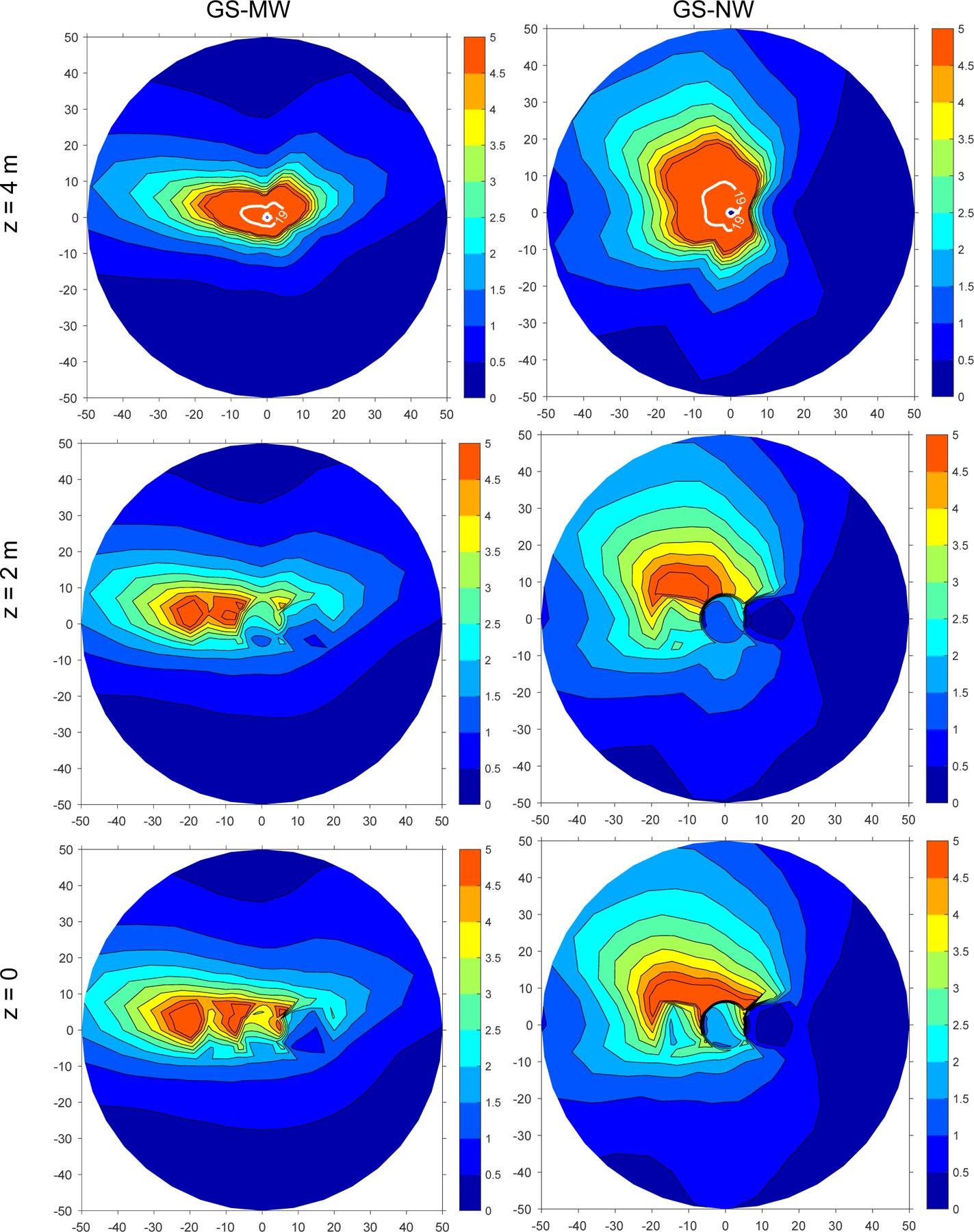
Modeled average benzene concentrations for GS-MW and GS-NW at three different elevations z. The x- and y-axes indicate horizontal coordinates in meters. The color indicates benzene levels in μg/m³ and the white isoline the MRL of 19 μg/m³ = 6 ppb.

Figure 7:

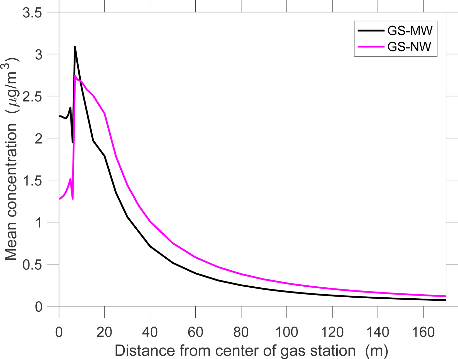
Mean benzene concentrations as a function of distance from the center of the gas stations.

5. DISCUSSION

5.1. Vent Emission Factors

We present unique data on vent emissions from USTs at two gas stations. Emissions can be compared to vent losses assumed by CAPCOA.²⁷ For a gas station with Stage I and II vapor recovery technology and a P/V valve on the vent pipe of the UST (Scenario 6B), the CAPCOA study assumed loading losses of 0.084 and breathing losses of 0.025 lb/kgal dispensed. The total loss of gasoline through the vent pipe is the sum of the two and amounts to a vent emission factor ${\text{EF}}_{\mathit{\text{vent}}}$ = 0.109 lb/kgal. Based on actual measurements in two fully functioning US gas stations, we obtained ${\text{EF}}_{\mathit{\text{vent}}}$ values of 1.4 lb/kgal for GS-MW and 1.7 lb/kgal for GS-NW, more than one order of magnitude higher than the CAPCOA estimate. While the difference between our measurements and the CAPCOA estimates may appear surprising, it is important to consider that the CAPCOA estimates are based on relatively few measurements and some unsupported assumptions,³³ particularly with regard to uncontrolled emissions due to equipment failures or defects (Appendix A-5²⁷).

5.2. Pressure Measurements

Tank ullage pressure p was moderately to strongly positively correlated with vent flow rate Q, likely because exceedance of the cracking pressure of the P/V valve causes a vent release. Thus pressure measurements can be used to infer vent releases. Real-time detection of equipment failures and leaks via so-called in-station diagnostics systems is based on our observed correlations between p and Q.

5.3. Diurnal Fluctuations in Vent Emissions

Diurnal vent emissions were quite different at the two gas stations. At GS-MW, a 24-hour operation, vent emissions were high during the daytime, presumably due to PWD. Emissions ceased at night, likely because less gasoline was dispensed and fuel deliveries with relatively cool product were frequent. Evaporative losses could also have been lower at night because the cooler delivered fuel would cause slight contraction of the liquid phase with corresponding growth in the ullage volume while at the same time lowering the vapor pressure of gasoline in the UST.

At GS-NW, vent pipe releases occurred most of the time, during the daytime when fuel was dispensed (PWD) and at night when the gas station was closed. Vent releases were higher when the gas station was closed, suggesting that during the day-time Stage II vapor recovery resulted in the injection of vapors into the storage tank that were not completely equilibrated with the liquid gasoline. During night-time, the gradual equilibration of unsaturated air in the ullage of the UST with gasoline vapors could then have caused exceedance of the cracking pressure of the P/V valve and consequently vapor release. It seems counterintuitive that less nighttime emissions occurred at the gas station where fuel was dispensed. However, while fuel is being dispensed, the outgoing liquid creates additional ullage volume, and depending on excess air ingestion rate, a negative pressure could result that lowers vent pipe emissions.

Dispensing fuel to customer vehicles and the associated Stage II vapor recovery system interact with vent emissions and can even cause vent emission during PWD, because the vacuum-assist method can negatively interfere with Onboard Refueling Vapor Recovery (ORVR) installed in customer vehicles.³⁴ However, Stage II vapor recovery is not obsolete. It can be used in conjunction with ORVR to minimize exposure of gas station customers and workers to benzene due to working losses,³⁵ particularly when customer vehicles are not equipped with ORVR (e.g., older vehicles, boats, motorcycles) or small volume gasoline containers are refueled. Enhanced Stage II vapor recovery technology can significantly reduce vapor emissions both at the nozzle and from UST vent pipes.³⁶

5.4. Fuel Deliveries and Accidental Vent Releases

Based on observations and interpretation of time series of the tank pressure data, it is likely that the peak vent emissions (e.g., Figure 3b) were partly due to non-compliant bulk fuel drops where the Stage I vapor recovery system either was not correctly hooked up by the delivery driver or to hardware problems with piping and/or valves. This conjecture is consistent with typical US storage tank volumes (~10,000 to 30,000 gal). Assuming that Phase I vapor recovery did not work at all and that 10,000 gal (~38,000 L) of fuel were delivered, the working loss (volume of gasoline vapor/air mixture released to the atmosphere through the vent pipe) is 38,000 L. It is also reasonable to assume that delivery lasted less than one hour. According to Table 2, the maximum hourly flow rate through the vent pipe was 250 L/min at GS-MW, which would result in a maximum cumulative vapor release of 15,000 L within this hour. The measured maximum cumulative release underestimates the assumed working loss of 38,000 L. This could be due to a fuel delivery, which involved dropping fuel from multiple compartments of a tanker truck, with the vapor return hose not being correctly hooked up for only some of the emptied compartments.

At GS-MW, UST pressure decreased after fuel delivery (causing vent emissions to cease for several hours) during the climatic conditions prevalent during the observation period, behavior not observed at GS-NW. In practice, it is possible to observe both positive and negative pressure excursions, even during the same fuel delivery (when multiple fuel compartments of tanker trucks are unloaded), when Stage I vapor recovery is in place (personal observation by TT).

5.5. Exceedance of 1-hour Exposure Limits

AERMOD air pollution modeling suggests that at GS-MW the 1-hour acute REL was exceeded at one grid point 160 m (525 ft) from the center of the gas station once in 20 days (Figure 5). This distance is larger than the 300-ft (91 m) setback distance recommended by CARB for a large gasoline dispensing facility.²⁶ Assuming the gas station’s fence line is less than 225 ft (69 m) from its center (where the vent pipe was assumed to be located), our study shows that sensitive land uses at a distance further than 300 feet from the fence line of the gas station would represent a health concern despite compliance with the CARB guidelines because of non-compliance with the acute REL.

At any location further than 50 m from the gas station’s center, the REL was exceeded at most once during the 20-day measurement campaign (Figure SI-1a). However, exceedance occurred at several locations, and on two different days (Figure SI-1b). E.g., at a distance of 120 m from the center, the REL was exceeded at three grid points, and the number of grid points increased with closer proximity to the gas station. This suggests that it was not just a single worst-case scenario or a single accidental vapor release that led to REL exceedance; rather exceedance may occur more frequently than is anticipated. Prevalent wind directions during the measurement campaign explained the directional patterns of exceedances (see the wind rose in Figure SI-3a).

At GS-NW, despite its higher sales volume, the REL was exceeded only closer than 50 m from the gas station’s center. However, exceedance occurred much more frequently (Figure SI-2), likely because of the higher sales volume of GS-NW. Again, the wind rose for GS-NW (Figure SI-3b) explains spatial patterns of REL exceedance.

None of AIHA’s three ERPG levels were exceeded, meaning that individuals, except perhaps sensitive members of the public, would not have experienced more than mild, transient adverse health effects.

5.6. Average Benzene Levels

The initial increase in average benzene levels when moving away from the gas stations’ centers (Figure 7) is likely due to the vent emissions (at 4 m) which represent the largest benzene source, and which require a certain transport distance until they reach the 2-m level through dispersion. Further away from the gas station, benzene levels are higher for GS-NW than for GS-MW likely because of the higher sales volume of GS-NW. However, close to the center, benzene levels are higher at GS-MW. This can be attributed to the higher wind speeds at GS-NW (Table SI-1), which result in greater initial dilution of emitted pollutants in the incoming airstream and also in greater subsequent pollutant dispersion.

Modeled average benzene concentrations are generally lower (~10 μg/m³ or less) than those measured in the surroundings of gas stations, likely because our simulations do not account for traffic-related air pollution (TRAP). For instance, a study published by the Canadian petroleum industry found average benzene concentrations of 146 and 461 ppb (466 and 1,473 μg/m³) at the gas station property boundary in summer and winter, respectively,³⁷ values orders of magnitudes higher than ours. A South Korean study examined outdoor and indoor benzene concentrations at numerous residences within 30 m and between 60 and 100 m of gas stations and found median outdoor benzene concentrations of 9.9 and 6.0 μg/m³, respectively,⁷ while we simulated benzene levels on the order of 1 μg/m³ (Figure 7). In a study on atmospheric BTEX levels in an urban area in Iran, the three highest BTEX levels were measured near gas stations (~150 m away); the measured benzene levels (64±36, 31±28, 52±26 μg/m³) were again much higher than ours simulated at that distance, likely due to TRAP. Our modeled average benzene levels at a distance of about 50 m are on the same order as background benzene levels of 1.0 μg/m³ that were measured in 2010 in the National Air Toxics Trend Sites (NATTS) network of 27 stations located in most major urban areas in the US.³⁸ However, our modeled levels at a distance of 170 m were 0.07 at GS-MW and 0.12 at GS-NW, a non-negligible addition to urban background levels.

At both gas stations, the MRL was exceeded at the level of the vent pipe opening in the vicinity of the gas stations, up to 7 m away from the vent pipe at GS-MW and 8 m at GS-NW. Therefore there might be an appreciable risk of adverse noncancer health effects for individuals living at the 2^nd-floor level relatively close to high-volume gas stations such as GS-MW and GS-NW.

5.7. Limitations

A limitation of our study is that data were collected only in fall and winter. Results cannot be easily extrapolated to other seasons, because vent pipe emissions are seasonally dependent, e.g., due to seasonally dependent gasoline formulations and meteorological conditions. However, modeled exceedance of the OEHHA acute REL in the winter season is already of concern, because that REL was developed for once per month or less exposures.

Another limitation is that we did not directly measure benzene levels in the vent pipe, and instead made assumptions about vapor composition that were also made in the CAPCOA study²⁷ of gas station emissions. In practice it may be difficult to obtain permission from gas station owners to measure benzene levels directly.

In part because we did not want to reveal the locations of the gas stations, we did not use site-specific topography information in the air dispersion modeling and instead assumed flat terrain. While this simplification results in less accurate air pollution predictions for the two sites, using a “generic” gas station is perhaps more representative of other gas station sites, and is consistent with an approach used in a previous study.²⁷

Finally, our study did not predict benzene levels in indoor environments. Even though indoor air pollution levels may substantially differ from outdoor levels due to indoor sources (e.g., smoking, photocopying),³⁹ our study can still inform exposure levels in indoor environments as outdoor sources may be the main contributors to indoor air pollution, e.g., in buildings situated in urban areas and close to industrial zones or streets with heavy traffic.⁴⁰ This is relevant to workers and customers in C-stores or other fast-food/gasoline station combination facilities.

6. CONCLUSIONS

Our study is to the best of our knowledge the first one to (1) report hourly vent emission data for gasoline storage tanks in the peer-reviewed literature and (2) use these data in hourly simulations of atmospheric benzene vapor transport. This allowed us to examine potential exceedance of short-term exposure limits for benzene. Prior studies including CAPCOA’s²⁷ could not do so as average emission rates were used (only meteorological data was used at an hourly resolution).

Our findings support the need to revisit setback distances for gas stations, which are based on more than 2-decade old estimates of vent emissions.³³ Also, CARB setback distances are based on a binary decision, related to whether the gasoline sales volume ${\dot{V}}_{\mathit{\text{sales}}}$ is more than 3.6 million gal per year. Our data support, however, that setback distances should be a continuous function of sales volume ${\dot{V}}_{\mathit{\text{sales}}}$ and also include the type of controls installed at the facility. Setback distances should also address health outcomes other than cancer. OEHHA’s acute REL for benzene could be used to inform setback distances as it accounts for non-cancer adverse health effects of benzene and its metabolites.⁴¹ ATSDR’s MRL could also be considered since it is a health-based limit.

We note that CARB recommended their setback distances in 2005, presumably assuming pollution prevention technology yielding a 90% reduction in benzene emissions.²⁶ Since then, CARB further promoted use of second-generation vapor recovery technology (Enhanced Vapor Recovery, EVR) to reduce emissions further. EVR includes technology that is supposed to prevent fuel vapors in overpressurized tanks from being expelled into the atmosphere.⁴² To that end, “bladder tanks” have been proposed, into which the gasoline vapor/air mixture is directed as the pressure in the combined ullage space of the storage tank increases and from which the mixture is redirected into the fuel storage tanks if the ullage pressure becomes negative (when fuel is dispensed). The challenge with such a system is to ensure that the bladder tank capacity is not exceeded by the fuel evaporation rate. Alternatively, fuel vapor release can be reduced by processing the fuel/air mixture through either a semi-permeable membrane which selectively exhausts clean air and returns enriched fuel vapor⁴³ or an activated carbon filter which adsorbs hydrocarbons (and water vapor) and exhausts air into the atmosphere, or by combusting the fuel/air mixture which would otherwise be released through the P/V valve. Therefore, current CARB setback distances might be adequate for gas stations in California but less so for the other 49 US states, and other countries—depending on pollution prevention technology requirements.

The larger areal extent of modeled REL exceedance at GS-MW is due to “accidental” releases of gasoline vapors. Even though regulations appear generally not to be driven by accidental releases, at GS-NW such releases likely led on two different days to REL exceedances at distances beyond CARB’s recommended setback distances. Policies should address accidental fuel vapor releases that depending on pollution prevention technology (here Stage I vapor recovery) and its proper functioning can occur on a frequent basis (twice at GS-MW within about three weeks).

In future work, potential exceedance of other shorter-term exposure limits should be examined, e.g., the 15-minute short-term exposure limits (STELs) and the 8-hour time-weighted averages (TWAs) used for occupational exposures.

REFERENCES

- 1.EIA. U.S. Product Supplied of Finished Motor Gasoline: U.S. Energy Information Administration; 2017. Available from: http://www.eia.gov/dnav/pet/hist/LeafHandler.ashx?n=pet&s=mgfupus1&f=m. [Google Scholar]
- 2.Hilpert M, Mora BA, Ni J, Rule AM, Nachman KE. Hydrocarbon Release During Fuel Storage and Transfer at Gas Stations: Environmental and Health Effects. Current Environmental Health Reports. 2015;2(4):412–22. doi: 10.1007/s40572-015-0074-8. [DOI] [PubMed] [Google Scholar]
- 3.ATSDR. Interaction Profile for: Benzene, Toluene, Ethylbenzene, and Xylenes (BTEX). Agency for Toxic Substances and Disease Registry, 2004. [PubMed] [Google Scholar]
- 4.IARC. IARC Monographs on the Evaluation of Carcinogenic Risks to Humans. Volume 100F 2012 [December 24, 2017]. Available from: http://monographs.iarc.fr/ENG/Monographs/vol100F/.
- 5.Terres IMM, Minarro MD, Ferradas EG, Caracena AB, Rico JB. Assessing the impact of petrol stations on their immediate surroundings. Journal of Environmental Management. 2010;91(12):2754–62. doi: 10.1016/j.jenvman.2010.08.009. [DOI] [PubMed] [Google Scholar]
- 6.Jo WK, Oh JW. Exposure to methyl tertiary butyl ether and benzene in close proximity to service stations. Journal of the Air & Waste Management Association. 2001;51(8):1122–8. doi: 10.1080/10473289.2001.10464339. [DOI] [PubMed] [Google Scholar]
- 7.Jo WK, Moon KC. Housewives’ exposure to volatile organic compounds relative to proximity to roadside service stations. Atmospheric Environment. 1999;33(18):2921–8. doi: 10.1016/s1352-2310(99)00097-7. [DOI] [Google Scholar]
- 8.Hajizadeh Y, Mokhtari M, Faraji M, Mohammadi A, Nemati S, Ghanbari R, Abdolahnejad A, Fard RF, Nikoonahad A, Jafari N, Miri M. Trends of BTEX in the central urban area of Iran: A preliminary study of photochemical ozone pollution and health risk assessment. Atmospheric Pollution Research. 2018;9(2):220–9. [Google Scholar]
- 9.Infante PF. Residential Proximity to Gasoline Stations and Risk of Childhood Leukemia. American Journal of Epidemiology. 2017;185(1):1–4. [DOI] [PMC free article] [PubMed] [Google Scholar]
- 10.Steffen C, Auclerc MF, Auvrignon A, Baruchel A, Kebaili K, Lambilliotte A, Leverger G, Sommelet D, Vilmer E, Hemon D, Clavel J. Acute childhood leukaemia and environmental exposure to potential sources of benzene and other hydrocarbons; a case-control study. Occupational and Environmental Medicine. 2004;61(9):773–8. doi: 10.1136/oem.2003.010868. [DOI] [PMC free article] [PubMed] [Google Scholar]
- 11.Brosselin P, Rudant J, Orsi L, Leverger G, Baruchel A, Bertrand Y, Nelken B, Robert A, Michel G, Margueritte G, Perel Y, Mechinaud F, Bordigoni P, Hemon D, Clavel J. Acute childhood leukaemia and residence next to petrol stations and automotive repair garages: the ESCALE study (SFCE). Occupational and Environmental Medicine. 2009;66(9):598–606. [DOI] [PubMed] [Google Scholar]
- 12.Harrison RM, Leung PL, Somervaille L, Smith R, Gilman E. Analysis of incidence of childhood cancer in the West Midlands of the United Kingdom in relation to proximity to main roads and petrol stations. Occupational and Environmental Medicine. 1999;56(11):774–80. [DOI] [PMC free article] [PubMed] [Google Scholar]
- 13.Hilpert M, Breysse PN. Infiltration and evaporation of small hydrocarbon spills at gas stations. Journal of Contaminant Hydrology. 2014;170:39–52. [DOI] [PubMed] [Google Scholar]
- 14.Mora BA, Hilpert M. Differences in Infiltration and Evaporation of Diesel and Gasoline Droplets Spilled onto Concrete Pavement. Sustainability. 2017;9(7). doi: 10.3390/su9071271. [DOI] [Google Scholar]
- 15.Morgester JJ, Fricker RL, Jordan GH. Comparison of spill frequencies and amounts at vapor recovery and conventional service stations in California. Journal of the Air & Waste Management Association. 1992;42(3):284–9. [Google Scholar]
- 16.Yerushalmi L, Rastan S. Evaporative Losses from Retail Gasoline Outlets and Their Potential Impact on Ambient and Indoor Air Quality In: Li A, Zhu Y, Li Y, editors. Proceedings of the 8th International Symposium on Heating, Ventilation and Air Conditioning: Volume 1: Indoor and Outdoor Environment. Berlin, Heidelberg: Springer Berlin Heidelberg; 2014. p. 13–21. [Google Scholar]
- 17.Statistics Canada. Gasoline Evaporative Losses from Retail Gasoline Outlets Across Canada: Environment Accounts and Statistics Analytical and Technical Paper Series; 2009. Available from: http://www.statcan.gc.ca/pub/16-001-m/2012015/part-partie1-eng.htm.
- 18.EPA. Transportation and Marketing of Petroleum Liquids. Environmental Protection Agency, 2008 AP 42, Volume I, Chapter V: Petroleum Industry. [Google Scholar]
- 19.McEntire BR. Performance of Balance Vapor Recovery Systems at Gasoline Dispensing Facilities. San Diego Air Pollution Control District, 2000. [Google Scholar]
- 20.Atabi F, Mirzahosseini SA. GIS-based assessment of cancer risk due to benzene in Tehran ambient air. Int J Occup Med Environ Health. 2013;26(5):770–9. Epub 2014/01/28. doi: 10.2478/s13382-013-0157-4. [DOI] [PubMed] [Google Scholar]
- 21.Correa SM, Arbilla G, Marques MRC, Oliveira KMPG. The impact of BTEX emissions from gas stations into the atmosphere. Atmospheric Pollution Research. 2012;3(2):163–9. [Google Scholar]
- 22.Cruz L, Alves L, Santos A, Esteves M, Gomes Í, Nunes L. Assessment of BTEX Concentrations in Air Ambient of Gas Stations Using Passive Sampling and the Health Risks for Workers. Journal of Environmental Protection. 2007;8:12–25. [Google Scholar]
- 23.Edokpolo B, Yu QJ, Connell D. Health risk characterization for exposure to benzene in service stations and petroleum refineries environments using human adverse response data. Toxicology Reports. 2015;2:917–27. [DOI] [PMC free article] [PubMed] [Google Scholar]
- 24.Edokpolo B, Yu QJ, Connell D. Health Risk Assessment of Ambient Air Concentrations of Benzene, Toluene and Xylene (BTX) in Service Station Environments. International Journal of Environmental Research and Public Health. 2014;11(6):6354–74. [DOI] [PMC free article] [PubMed] [Google Scholar]
- 25.Karakitsios SP, Delis VK, Kassomenos PA, Pilidis GA. Contribution to ambient benzene concentrations in the vicinity of petrol stations: Estimation of the associated health risk. Atmospheric Environment. 2007;41(9):1889–902. [Google Scholar]
- 26.CalEPA/CARB. Air Quality and Land Use Handbook: A Community Health Perspective: California Environmental Protection Agency & California Air Resources Board; 2005. [Google Scholar]
- 27.CAPCOA. Gasoline Service Station Industrywide Risk Assessment Guidelines. Toxics Committee of the California Air Pollution Control Officers Association (CAPCOA), 1997. [Google Scholar]
- 28.WHO. WHO Guidelines for Indoor Air Quality: Selected Pollutants: Geneva: World Health Organization; 2010. [PubMed] [Google Scholar]
- 29.AIHA. 2016 ERPG/WEEL Handbook. Current ERPG® Values (2016): American Industrial Hygiene Association; 2016. [Google Scholar]
- 30.ATSDR. Minimal Risk Levels (MRLs): Agency for Toxic Substances and Disease Registry; 2018 [May 24, 2018]. Available from: https://www.atsdr.cdc.gov/mrls/index.asp. [Google Scholar]
- 31.Cimorelli AJ, Perry SG, Venkatram A, Weil JC, Paine RJ, Wilson RB, Lee RF, Peters WD, Brode RW. AERMOD: A Dispersion Model for Industrial Source Applications. Part I: General Model Formulation and Boundary Layer Characterization. Journal of Applied Meteorology. 2005;44(5):682–93. [Google Scholar]
- 32.ATSDR. Toxicological Profile for Benzene. Agency for Toxic Substances and Disease Registry, 2007. CAS#: 71-43-2. [PubMed] [Google Scholar]
- 33.Aerovironment I. Underground Storage Tank Vent Line Emissions form Retail Gasoline Outlets. Prepared for WSPA, 1994. AV-FR-92-01-204R2. [Google Scholar]
- 34.EPA. Stage II Vapor Recovery Systems Issues Paper. U.S. EPA. Office of Air Quality Planning and Standards Emissions Monitoring and Analysis Division. Emissions Factors and Policy Applications Group (D243–02), 2004. [Google Scholar]
- 35.Cruz-Nunez X, Hernandez-Solis JM, Ruiz-Suarez LG. Evaluation of vapor recovery systems efficiency and personal exposure in service stations in Mexico City. Science of the Total Environment. 2003;309(1–3):59–68. doi: 10.1016/s0048-9697(03)00048-2. [DOI] [PubMed] [Google Scholar]
- 36.CARB. Revised Emission Factors for Gasoline Marketing Operations at California Gasoline Dispensing Facilities. California Air Resources Board, Monitoring and Laboratory Division, 2013. [Google Scholar]
- 37.Akland GG. Exposure of the general population to gasoline. Environ Health Perspect. 1993;101 Suppl 6:27–32. Epub 1993/12/01. [DOI] [PMC free article] [PubMed] [Google Scholar]
- 38.Strum M, Scheffe R. National review of ambient air toxics observations. Journal of the Air & Waste Management Association (1995). 2016;66(2):120–33. Epub 2015/08/01. doi: 10.1080/10962247.2015.1076538. [DOI] [PubMed] [Google Scholar]
- 39.El-Hashemy MA, Ali HM. Characterization of BTEX group of VOCs and inhalation risks in indoor microenvironments at small enterprises. Science of The Total Environment. 2018;645:974–83. [DOI] [PubMed] [Google Scholar]
- 40.Jones AP. Indoor air quality and health. Atmospheric Environment. 1999;33(28):4535–64. [Google Scholar]
- 41.Budroe J Notice of Adoption of Revised Reference Exposure Levels for Benzene: Office of Environmental Health Hazard Assessment (California, US); 2014. Available from: https://oehha.ca.gov/air/crnr/notice-adoption-revised-reference-exposure-levels-benzene.
- 42.CARB. Public Workshop to Discuss: Overpressure Conditions at Gasoline Dispensing Facilities Equipped with Underground Storage Tanks and Phase II Enhanced Vapor Recovery including In-Station Diagnostic Systems. December 12–13, 2017. Diamond Bar & Sacramento, CA: California Air Resources Board; 2017. Available from: https://www.arb.ca.gov/vapor/op/wrkshps/dec2017op_vr_pres.pdf. [Google Scholar]
- 43.Semenova SI. Polymer membranes for hydrocarbon separation and removal. Journal of Membrane Science. 2004;231(1–2):189–207. [Google Scholar]
- 44.EPA. Gasoline Mobile Source Air Toxics 2017. Available from: https://www.epa.gov/gasoline-standards/gasoline-mobile-source-air-toxics. [Google Scholar]
- 45.EPA. Air Quality: Widespread Use for Onboard Refueling Vapor Recovery and Stage II Waiver2012;Federal Register 40 CFR 51:28772–82. [Google Scholar]
Associated Data
This section collects any data citations, data availability statements, or supplementary materials included in this article.