A disk-aware algorithm for time series motif discovery

Abstract

Time series motifs are sets of very similar subsequences of a long time series. They are of interest in their own right, and are also used as inputs in several higher-level data mining algorithms including classification, clustering, rule-discovery and summarization. In spite of extensive research in recent years, finding time series motifs exactly in massive databases is an open problem. Previous efforts either found approximate motifs or considered relatively small datasets residing in main memory. In this work, we leverage off previous work on pivot-based indexing to introduce a disk-aware algorithm to find time series motifs exactly in multi-gigabyte databases which contain on the order of tens of millions of time series. We have evaluated our algorithm on datasets from diverse areas including medicine, anthropology, computer networking and image processing and show that we can find interesting and meaningful motifs in datasets that are many orders of magnitude larger than anything considered before.

1. Introduction

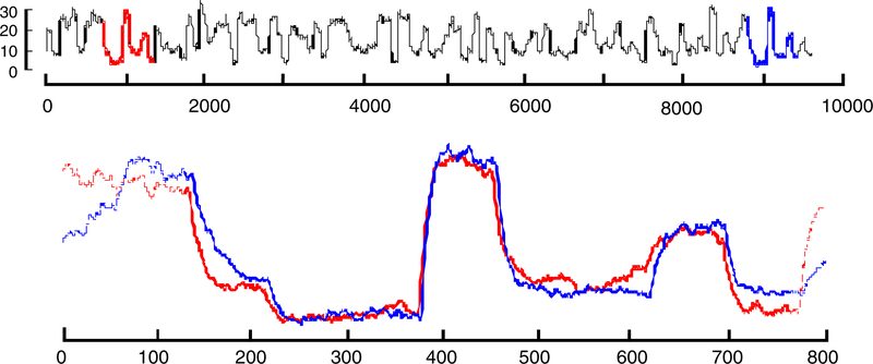
Time series motifs are sets of very similar subsequences of a long time series, or from a set of time series. Fig. 1 illustrates an example of a motif discovered in an industrial dataset. As in other domains, (i.e. text, DNA, video Cheung and Nguyen 2005) this approximately repeated structure may be conserved for some reason that is of interest to the domain specialists. In addition, time series motifs are also used as inputs in several higher-level data mining algorithms, including classification (Mueen et al. 2009), clustering, rule-discovery and summarization. Since their formalization in 2002, time series motifs have been used to solve problems in domains as diverse as human motion analyses, medicine, entertainment, biology, anthropology, telepresence and weather prediction.

Fig. 1.

(Top) The output steam flow telemetry of the Steamgen dataset has a motif of length 640 beginning at locations 589 and 8,895. (Bottom) By overlaying the two motifs we can see how remarkably similar they are to each other

In spite of extensive research in recent years (Chiu et al. 2003; Ferreira et al. 2006; Mueen et al. 2009; Yankov et al. 2007), finding time series motifs exactly in massive databases is an open problem. Previous efforts either found approximate motifs or considered relatively small datasets residing in main memory (or in most cases, both). However, in many domains we may have datasets that cannot fit in main memory. For example, in this work we consider a 228GB dataset. We must somehow find the motif in this dataset, while only allowing a tiny fraction (less than 1%) of it in main memory at any one time. In this work, we describe for the first time a disk-aware algorithm to find time series motifs in multi-gigabyte databases containing tens of millions of time series. As we shall show, our algorithm allows us to tackle problems previously considered intractable, for example finding near duplicates in a dataset of forty-million images.

The rest of this paper is organized as follows. In Sect. 2 we review related work. In Sect. 3 we introduce the necessary notation and background to allow the formal description of our algorithm in Sect. 4. Sections. 5 and 6 empirically evaluate the scalability and utility of our ideas, and we conclude with a discussion of future work in Sect. 7.

2. Related work

Many of the methods for time series motif discovery are based on searching a discrete approximation of the time series, inspired by and leveraging off the rich literature of motif discovery in discrete data such as DNA sequences (Chiu et al. 2003; Patel et al. 2002; Ferreira et al. 2006; Minnen et al. 2007a; Yoshiki et al. 2005; Simona and Giorgio 2004). Discrete representations of the real-valued data must introduce some level of approximation in the motifs discovered by these methods. In contrast, we are interested in finding motifs exactly with respect to the raw time series. More precisely, we want to do an exact search for the most similar pair of subsequences (i.e. the motif) in the raw time series. It has long been held that the exact discovery of motif is intractable even for datasets residing in main memory. In a recent work the current authors have shown that motif discovery is tractable for large in-core datasets (Mueen et al. 2009); however, in this work we plan to show that motif discovery can be made tractable even for massive disk resident datasets.

The literature is replete with different ways of defining time series “motifs.” Motifs are defined and categorized using their support, distance, cardinality, length, dimension, underlying similarity measure, etc. Motifs may be restricted to have a minimum count of participating similar subsequences (Chiu et al. 2003; Ferreira et al. 2006) or may only be a single closest pair (Mueen et al. 2009). Motifs may also be restricted to have a distance lower than a threshold (Chiu et al. 2003; Ferreira et al. 2006; Yankov et al. 2007), or restricted to have a minimum density (Minnen et al. 2007b). Most of the methods find fixed length motifs (Chiu et al. 2003; Ferreira et al. 2006; Mueen et al. 2009; Yankov et al. 2007), while there are a handful of methods for variable length motifs (Minnen et al. 2007b; Yoshiki et al. 2005; Tang and Liao 2008). Multi-dimensional motifs and subdimensional motifs are defined (Minnen et al. 2007a) and heuristic methods to find them are explored in (Minnen et al. 2007a,b; Yoshiki et al. 2005). Depending on the domain in question, the distance measures used in motif discovery can be specialized, such as allowing for “don’t cares” to increase tolerance to noise (Chiu et al. 2003; Simona and Giorgio 2004). In this paper we explicitly choose to consider only the simplest definition of a time series motif, which is the closest pair of time series subsequences of fixed length. Since virtually all of the above definitions can be trivially calculated with inconsequential overhead using the closest pair as a seed, we believe the closest pair is the core operation in motif discovery. Therefore, we ignore other definitions for brevity and simplicity of exposition.

To the best of our knowledge, the closest-pair/time series motif problem in high dimensional (i.e. hundreds of dimensions) disk resident data has not been addressed. There has been significant work on spatial closest-pair queries (Nanopoulos et al. 2001; Corral et al. 2000). These algorithms used indexing techniques such as R-tree and R*-tree which have the problem of high creation and maintenance cost for multi-dimensional data (Koudas and Sevcik 2000). In Weber et al. (1998), it has been proved that there is a dimensionality beyond which every partitioning method (R*-tree, X-tree, etc.) degenerates into sequential access. Another possible approach could be to use efficient high dimensional self similarity join algorithms (Koudas and Sevcik 2000; Dohnal et al. 2003). If the data in hand is joined with itself with a low similarity threshold we would get a motif set, which could be quickly refined to find the true closest pair. However, the threshold must be at least as big as the distance between the closest pair to filter it from the self-join results. This is a problem because most of the time users do not have any idea about a good threshold value. Obviously, user can choose a very large threshold for guaranteed results, but this degrades the performance a lot. In this regard, our method is parameter free and serves the exact purpose of finding the closest pair of time series. Besides, the datasets we wish to consider in this work have three orders of magnitude more objects than any of the datasets considered in Corral et al. (2000); Koudas and Sevcik (2000); Nanopoulos et al. (2001) and dimensionality (i.e length) of the motifs are from several hundreds to a thousand whereas in Koudas and Sevcik (2000) the maximum dimensionality is thirty. Therefore, our algorithm is the first algorithm to find exact time series motifs in disk resident data.

Given this, most of the literature has focused on fast approximate algorithms for motif discovery (Beaudoin et al. 2008; Chiu et al. 2003; Minnen et al. 2007b; Tanaka et al. 2005; Guyet et al. 2007; Meng et al. 2008; Rombo and Terracina 2004; Lin et al. 2002). For example, a recent paper on finding approximate motifs reports taking 343s to find motifs in a dataset of length 32,260 (Meng et al. 2008), in contrast we can find motifs in similar datasets exactly, and on similar hardware in under 100s. Similarly, another very recent paper reports taking 15min to find approximate motifs in a dataset of size 111,848 (Beaudoin et al. 2008), however we can find motifs in similar datasets in under 4min. Finally, paper (Liu et al. 2005) reports 5s to find approximate motifs in a stock market dataset of size 12,500, whereas our exact algorithm takes less than 1s.

It has long been known that the closest pair problem in multidimensional data has a lower bound of Ω (nlogn). The optimal algorithm is derived from the divide-and-conquer paradigm and exploits two properties of a dataset: sparsity of the data and the ability to select a “good” cut plane (Bentley 1980). This algorithm recursively divides the data by a cut plane. At each step it projects the data to the cut plane to reduce the dimensionality by one and then solve the subproblems in the lower dimensional space. Unfortunately the optimal algorithm hides a very high constant factor in the complexity expression, which is of the order of 2^d and the sparsity condition does not hold for time series subsequences (c.f. sect. 5.1). In addition, the large worst-case memory requirement and essentially random data accesses made the algorithm impractical for disk-resident applications.

In this paper we employ a bottom-up search algorithm that simulates the merge steps of the divide-and-conquer approach. Our contribution is that we created an algorithm whose worst-case memory and I/O overheads are practical for implementation on very large-scale databases. The key difference with the optimal algorithm that makes our algorithm amenable for large databases is that we divide the data without reducing the number of dimensions and without changing the data order at any divide step. This allows us to do a relatively small number of batched sequential accesses, rather than a huge number of random accesses. As we shall see, this can make a three- to four-order-of-magnitude difference in the time it takes to find the motifs on disk-resident datasets.

To the best of our knowledge, our algorithm is completely novel. However we leverage off related ideas in the literature (Gonzalez et al. 2008; Jagadish et al. 2005; Yu and Wang 2007). In particular, the iDistance method of Jagadish et al. (2005) introduces the idea of projecting data on to a single line, a core subroutine in our algorithm. Other works, for example Gonzalez et al. (2008) also exploits the information gained by the relative distances to randomly chosen reference points. However they use this information to solve the approximate similarity search problem, whereas we use it to solve the exact closest-pair problem. In Jagadish et al. (2005) and Yu and Wang (2007), Reference objects have been used for each partition of a B+ tree index which is adapted for different data distribution. However, we use only one reference object to do the data ordering. In Dohnal et al. (2003), Reference objects (pivots) are used to build an index for similarity joins. While we exploit similar ideas, the design of the index is less useful for the closest-pair problem because of data replication and parameter setting described previously. Both Jagadish et al. (2005) and Yu and Wang (2007) use the idea of pivots to do K-nearest neighbor search, and report approximately one order of magnitude speedup over brute force. However we use the idea of pivots for motif discovery and report four to five orders or magnitude. What explains this dramatic difference in speedup? A small fraction can be attributed to the simple fact that we consider significantly larger datasets, and pivot-based pruning is more effective for larger datasets. However, most of the difference can be explained by our recent observation that the speed up of pivot-based indexing depends on the value of the best-so-far variable (Mueen et al. 2009). While this value does decrease with datasets size for K-nearest neighbor search or full joins (Dohnal et al. 2003), it decreases much faster for motif discovery (Mueen et al. 2009), allowing us to prune over 99.99% of distance calculations for real-world problems.

3. Definition and background

As described in the previous section we focus on the simplest “core” definition of time series motifs. In this section we define the terms formally.

Definition 1

A time series is a sequence T = (t₁,t₂,...,t_m) of m real valued numbers.

The sequence of real valued numbers (t_i) is generally a temporal ordering. Other well-defined orderings such as shapes (Yankov et al. 2007), spectrographs, handwritten text, etc. can also be fruitfully considered as “time series.” As with most time series data mining algorithms, we are interested in local, not global properties of the time series and therefore, we need to extract subsequences from it.

Definition 2

A subsequence of length n of a time series T = (t₁,t₂,...,t_m) is a time series T_i,n = (t_i,t_i+1,...,t_i+n−1) for 1 ≤ i ≤ m − n + 1.

A time series of length m has m − n + 1 subsequences of length n. We naturally expect that adjacent subsequences will be similar to each other; these subsequences are known as trivial matches (Chiu et al. 2003). However, subsequences which are similar to each other, yet at least some minimum value w apart suggest a recurring pattern, an idea we formalize as a time series motif.

Definition 3

The time series motif is a pair of subsequences {T_i,n, T_j,n} of a long time series T of length m that is the most similar. More formally, the pair {T_i,n, T_j,n}, where $|i-j|\ge w,$ is the time series motif iff ∀a, b dist (T_i,n, T_j,n) ≤ dist(T_a,n, T_b,n), for $|a-b|\ge w$ and w > 0.

Note the inclusion of the separation window w. This means that a motif must contain subsequences separated by at least w positions. The reason behind this separation constraint is to prevent trivial matches from being reported as motif (Patel et al. 2002). To explain what is a trivial match, let us consider an example (on discrete data for simplicity). If we were looking for motifs of length four in the string:

$$\text{sjdbbnvfdfpqoeutyvnAB}\mathbf{AB}\text{ABmbzchslfkeruyousjdq}$$ (1)

Then, in this case we probably would not want to consider the pair {ABAB,ABAB} to be a motif, since they share 50% of their length (i.e AB is common to both). Instead, we would find the pair {sjdb, sjdq} to be a more interesting approximately repeated pattern.In this example, we can enforce this by setting the parameter $w=4.$ Therefore, after discounting trivial matches, the total number of possible motif pairs is exactly $\frac{(m-n-w+1)(m-n-w)}{2}.$

There are a number of distance measures to capture the notion of similarity between subsequences. In Ding et al. (2008) and elsewhere it has been empirically shown that simple Euclidean distance is competitive or superior to many of the complex distance measures and has the very important triangular inequality property. Note, however, that our method can work with any distance measure that is metric. Additional reasons for using Euclidean distance are that it is parameter-free and its calculation allows many optimizations, for example, it is possible to abandon the Euclidean distance computation as soon as the cumulative sum goes beyond the current best-so-far, an idea known as early abandoning (Mueen et al. 2009). For example assume the current best-so-far has a Euclidean distance of 12.0, and therefore a squared Euclidean distance of 144.0. If, as shown in Fig. 2, the next item to be compared is further away, then at some point the sum of the squared error will exceed the current minimum distance r=12.0 (or, equivalently r² = 144). So the rest of the computation can be abandoned since this pair can’t have minimum distance. Note that we work here with the squared Euclidean distance because we can avoid having to take square roots at each of the n steps in the calculation.

Fig. 2.

A visual intuition of early abandoning. Once the squared sum of the accumulated gray hatch lines exceeds r², we can be sure the full Euclidean distance exceeds r

One potential problem with Euclidean distance is that it is very sensitive to offset and scale (amplitude). Two subsequences of a time series may be very similar but at different offsets and/or scales, and thus report a larger distance than warranted. Normalization before comparison helps to mitigate this effect. In this paper, we use the standard z-normalization defined as $X=\frac{x-\mu }{\sigma }$ where X is the normalization of vector x with sample mean μ and standard deviation σ. Z-normalization is an O(n) operation. Therefore, to avoid renormalizing same subsequences multiple times, we compute all of the (m − n + 1) normalized subsequences just once, store all of them in a database of time series and use these normalized sequences when computing the distances.

Definition 4

A time series database is an unordered set of normalized time series or time series subsequences stored in one or multiple disk blocks of fixed or varying sizes.

Although the most typical applications of motif discovery involve searching subsequences of a long time series, one other possibility is that we may simply have m individual and independent time series to examine, such as m gene expression profiles or m star light curves. With the exception of the minor overhead of keeping track of the trivial matches (Chiu et al. 2003) in the former case, our algorithm is agnostic to which situation produces the time series and it assumes to have a time series database as the input and to output the time series motif found in the database.

As noted earlier, there are many other definitions of time series motifs (Lin et al. 2002; Yankov et al. 2007; Tang and Liao 2008; Minnen et al. 2007a). For example, we present two other useful definitions below.

Definition 5

The kth-TimeSeriesmoti f is the k most similar pair in the database D. The pair {T_i, T_j} is the kth motif iff there exists a set S of pairs of time series of size exactly k − 1 such that $\forall T_d\in D\left\{T_i,T_d\right\}\notin S\text{and}\left\{T_j,T_d\right\}\notin S\text{and}\forall \left\{T_x,T_y\right\}\in S,\left\{T_a,T_b\right\}\notin Sdist\left(T_x,T_y\right)\le dist\left(T_i,T_j\right)\forall dist\left(T_a,T_b\right).$

Definition 6

The Range motif with range r is the maximal set of time series that have the property that the maximum distance between them is less than 2r. More formally, S is a range motif with range $r\text{iff}\forall T_x,T_y\in Sdist\left(T_x,T_y\right)\le 2r$ and S is maximal.

In general, these definitions impose conditions on two major features of a set of subsequences: similarity and support. We note that all such conditions can easily be obtained with a single pass through the data using our definition as a seed. As such the Definition 3 above is the core task of time series motif discovery.

For example, suppose we are tasked with finding all the range motifs with range r. We can leverage of the simple observation that a necessary condition for a set S of time series to be a range motif is that any two of the time series must be within 2r of each other, and we can find such pairs using our algorithm. We can therefore simply do the following. Find the time series motif (as in Definition 3) and record the distance, dist(T_i,n, T_j,n). If the distance is greater than 2r, then we can report the null set as the answer to our query, and terminate. Otherwise, we do a linear scan through the data, retrieving all objects that are within 2r of both T_i,n, T_j,n. This set is a superset of the range motif, and we can trivially condense it to the correct set.

For meaningful motif discovery, the motif pair should be significantly more similar to each other than one would expect in a random database. In this work we gloss over the problem of assessing significance, other than to show that the motifs have an interpretation in the domains in question. In the next section we describe an algorithm which allows us to efficiently find the motifs in massive time series databases.

4. Our algorithm

A set of time series of length n can be thought of as a set of points in n-dimensional space. Finding the time series motif is then equivalent to finding the pair of points having the minimum possible distance between any two points. Before describing the general algorithm in detail, we present the key ideas of the algorithm with a simple example in two-dimensional space.

4.1. A detailed intuition of our algorithm

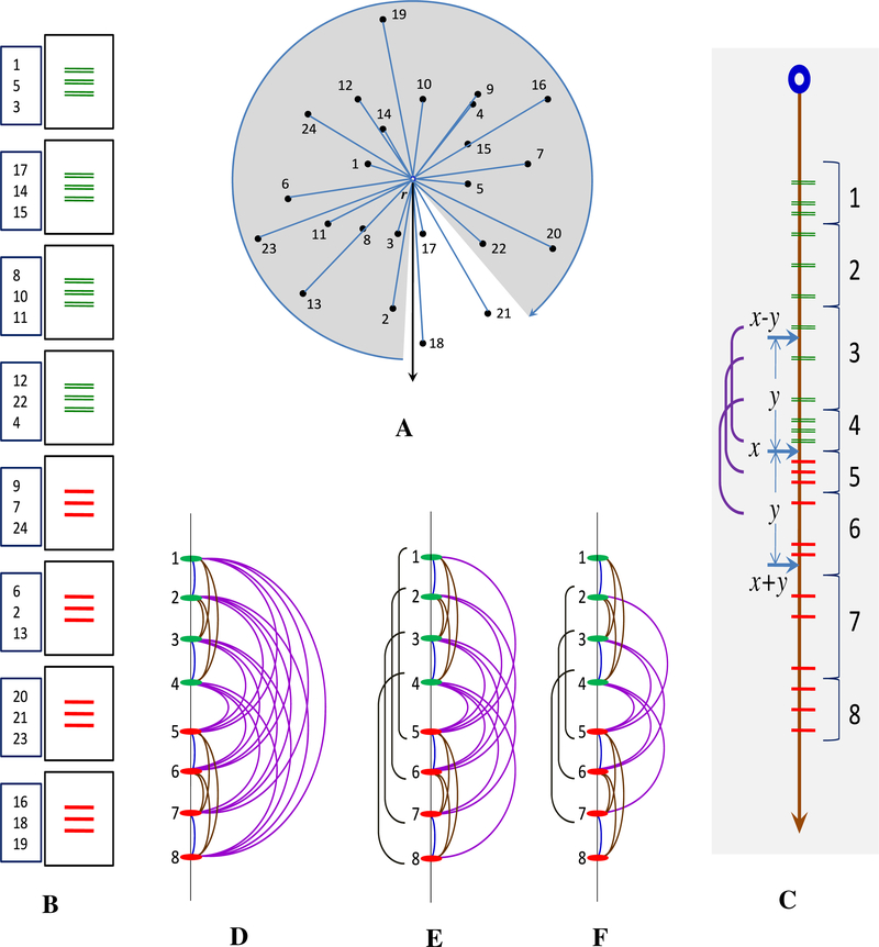
For this example, we will consider a set of 24 points in 2D space. In Fig. 3a the dataset is shown to scale. Each point is annotated by an id beside it. A moment’s inspection will reveal that the closest pair of points is {4,9}. We assume that a disk block can store at most three points (i.e. their co-ordinates) and their ids. So the dataset is stored in the disk in eight blocks.

Fig. 3.

a A sample database of 24 points. b Disk blocks containing the points sorted in the order of the distances from r. The numbers on the left are the ids. c All points projected on the order line. d A portion of an order line for a block of 8 points. e After pruning by a current motif distance of 4.0 units. f After pruning by 3.0 units

We begin by randomly choosing a reference point r (see Fig. 3a). We compute the distance of each data point from r and sort all such distances in ascending order. As the data is on the disk, any efficient external sorting algorithm can be used for this purpose (Motzkin and Hansen 1982; Nyberg et al. 1995). A snap shot of the database after sorting is shown in Fig. 3b. Note that our closest pair of points is separated in two different blocks. Point 4 is in the fourth block and point 9 is in the fifth block.

Geometrically, this sorting step can be viewed as projecting the database on one line by rotating all of the points about r and stopping when every point is on that line. We call this line the order line since it holds all of the points in the increasing order of their distances from r. The order line shown in Fig. 3c begins at the top, representing a distance of 0 from r and continues downward to a distance of infinity (note that the order line shown in Fig. 3c is representative, but does not strictly conform to the scale and relative distances of Fig. 3a). Data points residing in the same block after the sorting step are consecutive points in the order line and thus, each block has its own interval in the order line. In Fig. 3c the block intervals are shown beside the order line. Note that, up to this point, we have not compared any pairs of data points. The search for the closest pair (i.e. comparisons of pairs of points) will be done on this representation of the data.

Our algorithm is based upon the following observation. If two points are close in the original space, they must also be close in the order line. Unfortunately, the opposite is not true; two points which are very far apart in the original space might be very close in the order line. Our algorithm can be seen as an efficient way to weed out these false positives, leaving just the true motif.

As alluded to earlier, we search the database in a bottom-up fashion. At each iteration, we partition the database into consecutive groups. We start with the smallest groups of size 1 (i.e. one data point) and iteratively double the group size (i.e. 2,4,8,...). At each iteration, we take pairs of disjoint consecutive groups one at a time and compare all pairs of points that span those two groups. Fig. 3d shows a contrived segment of an order line unrelated to our running example, where a block of eight points is shown. An arc in this figure represents a comparison between two points. The closest four arcs to the order line {(1,2),(3,4),(5,6),(7,8)} are computed when the group size is 1. The following eight arcs {(1,3),(1,4),(2,3),(2,4),(5,7),(5,8),(6,7),(6,8)} are computed when the group size is 2 and the rightmost 16 arcs are computed when the group size is 4. Note that each group is compared with one of its neighbors in the order line at each iteration. After the in-block searches are over, we move to search across blocks in the same way. We start by searching across disjoint consecutive pairs of blocks and continually increasing the size of groups like 2 blocks, 4 blocks, 8 blocks, and so on. Here we encounter the issue of accessing the disk blocks efficiently, which is discussed later in this section.

As described thus far, this is clearly a brute force algorithm that will eventually compare all possible pairs of objects. However, we can now explain how the order line helps to prune the vast majority of the calculations.

Assume A and B are two objects, and B lies beyond A in the order line; in other words, dist(A,r) ≤ dist(B,r). By the triangular inequality we know that dist(A, B) ≥ dist(B,r) − dist(A,r). But dist(B,r) − dist(A,r) is the distance between A and B in the order line. Thus, the distance between two points in the order line is a lower bound on the true distance between them. Therefore, at some point during the search, if we know that the closest pair found so far has a distance of y, we can safely ignore all pairs of points that are more than y apart on the order line. For example, in Fig. 3e, if we know that the distance between the best pair discovered so far is 4.0 units, we can prune off comparisons between points {(1,6),(1,7),(1,8),(2,7),(2,8),(3,8)}, since they are more than 4.0 units apart on the order line. Similarly, if the best pair discovered so far had an even tighter distance of 3.0 units, we would have pruned off four additional pairs (see Fig. 3f).

More critically, the order line also helps to minimize the number of disk accesses while searching across blocks. Let us assume that we are done searching all possible pairs (i.e. inside and across blocks) in the top four blocks and also in the bottom four blocks (see Fig. 3b). Let us further assume that the smaller of the minimum distances found in each of the two halves is y. Let x be the distance of the cut point between the two halves from r. Now, all of the points lying within the interval (x − y, x] in the order line may need to be compared with at least one point from the interval [x, x + y). Points outside these two intervals can safely be ignored because they are more than y apart from the points in the other half. Since in Fig. 3c the interval (x − y, x] overlaps with the intervals of blocks 3 and 4 and the interval [x, x + y) overlaps with the intervals of blocks 5 and 6, we need to search points across block pairs {3,5}, {3,6}, {4,5} and {4,6}. Note that we would have been forced to search all 16 possible block pairs from the two halves if there were no order line.

Given that we are assuming the database will not fit in the main memory, the question arises as to how we should load these block pairs when the memory is very small. In this work, we assume the most restrictive case, where we have just the memory available to store exactly two blocks. Therefore, we need to bring the above four block pairs {{3,5}, {3,6}, {4,5}, {4,6}} one at a time. The number of I/O operations depends on the order in which the block pairs are brought into the memory. For example, if we search the above four pairs of blocks in that order, we would need exactly six block I/Os: two for the first pair, one for the second pair since block 3 is already in the memory, two for the third pair and one for the last pair since block 4 is already in the memory. If we choose the order {{3,5}, {4,6}, {3,6}, {4,5}} we would need seven I/Os. Similarly, if we chose the order {{3,5}, {4,5}, {4,6}, {3,6}}, we would need five I/Os. In the latter two cases there are reverse scans; a block (4) is replaced by a previous block (3) in the order line. We will avoid reverse scans and avail of sequential loading of the blocks to get maximum help from the order line.

To complete the example, let us seehow the order line helps in pruning pairs across blocks. When we have two blocks in the memory, we need to compare each point in one block to each point in the other block. In our running example, during the search across the block pair {3,6}, the first and second data points in block 3 (i.e. 8 and 10 in the database) have distances larger than y to any of the points in block 6 in the order line (see Fig. 3c). The third point (i.e. 11) in block 3 has only the first point (i.e. 6) in block 6 within y in the order line. Thus, for block pair {3,6}, instead of computing distances for all nine pairs of data points we would need to compute the distance for only one pair, $\langle 11,6\rangle .$

At this point, we have informally described how a special ordering of the data can reduce block I/Os as well as reduce pair-wise distance computations. With this background, we hope the otherwise daunting detail of the technical description in the next section will be less intimidating.

4.2. A formal description of our algorithm

For the ease of description, we assume the number of blocks (N) and the block size (m) are restricted to be powers of two. We also assume that all blocks are of the same size and that the main memory stores only two disk blocks with a small amount of extra space for the necessary data structures. Readers should note that in the pseudocode, all variable and method names are in italics and globally accessible elements are in bold. Shaded lines denote the steps for the pruning of pairs from being selected or compared. We call our algorithm DAME which is an abbreviated form of Disk Aware Motif Enumeration.

Our algorithm is logically divided into subroutines with different high-level tasks. The main method that employs the bottom-up search on the blocks is DAME_Motif shown in Table 1. The input to this method is a set of blocks B which contains every subsequence of a long time series or a set of independent time series. Each time series is associated with an id used for finding its location back in the original data. Individual time series are assumed to be z-normalized. If they are not, this is done in the sorting step.

Table 1.

DAME_Motif is the bottom up search procedure for disk blocks

Procedure DAME_Motif   (B)
B: array of disk blocks containing time series
L1,L2: Indices of the motif pair
bsf: The smallest distance
1	bsf ← INF, L1 ← −1 L2 ← −1
2	Dref ← Randomly pick r time series
3	r ← Dref1
4	sort(B,r)
5	s,e ← computeInterval(B)
6	t ← 1
7	while $t\le \frac{N}{2}$
8	top ← 1
9	while top < N
10	mid ← top+t
11	bottom ← top+2t
12	searchAcrossBlocks(top, mid, bottom)
13	top ← bottom
14	t ← 2t

DAME_Motif first chooses r random time series as reference points from the database and stores them in Dref. These reference time series can be from the same block, allowing them to be chosen in a single disk access. DAME_Motif then sorts the entire database, residing on multiple blocks, according to the distances from the first of the random references named as r. The reason for choosing r random reference time series/points will be explained shortly. The computeInterval method at line 5 in Table 1 computes the intervals of the sorted blocks. For example, if s_i and e_i are respectively the smallest and largest of the distances from r to any time series in B_i, then [s_i, e_i] is the block interval of B_i. Computing these intervals is done during the sorting phase, which saves a few disk accesses. Lines 7–14 detail the bottom-up search strategy. Let t be the group size, which is initialized to one, and iteratively doubled until it reaches $\frac{N}{2}.$ For each value of t, pairs of time series across pairs of successive t-groups are searched using the searchAcrossBlock method shown in Table 2.

Table 2.

searchAcrossBlocks compares pairs among disjoint set of blocks

Procedure  searchAcrossBlocks (top,mid,bottom)
top, mid, bottom: indices of the array of disk blocks, B
1	for p ← top to mid-1
2	if smid − ep ≥ bsf and mid-top != 1
3	continue
4	D1,Dist1 ← load(Bp)
5	if mid-top = 1
6	searchlnBlock(D1,Dist1)
7	istart ← 0
8	for q ← mid to bottom-1
9	if sq − ep ≥ bsf and bottom-mid != 1
10	break
11	D2,Dist2 ← load(Bq)
12	if bottom-mid = 1
13	searchInBlock (D2,Dist2)
14	for i ← istart + 1 to m
15	for j ← l to m
16	if Dist11,i − Dist21,j < bsf
17	update(Dl,D2,Distl,Dist2,i,j)
18	else
19	istart ← i
20	break

The searchAcrossBlocks method searches for the closest pair across the partitions [top,mid) and [mid,bottom). The order of loading blocks is straightforward (lines 1 and 8). The method sequentially loads one block from the top partition, and for each of them it loads all of the blocks from the bottom partition one at a time (lines 4 and 11). D1 and D2 are the two memory blocks and are dedicated for the top and bottom partitions, respectively. A block is loaded to one of the memory blocks by the load method shown in Table 3. load reads and stores the time series and computes the distances from the references.

Table 3.

load loads a disk block and computes the referenced distances

Procedure  load(b)
b:An index of the array of disk blocks, B
1	D ← read(b)
2	for i ← 1 to R
3	for j ← 1 to m
4	Disti,j ← dist(Drefi,Dj)
5	return D,Dist

DAME_Motif and all subroutines shown in Tables 1, 2, 3, 4, and 5 maintain a variable bsf (best so far) that holds the minimum distance discovered up to the current point of search. We define the distance between two blocks p and q by s_q − e_p if p < q. Lines 2–3 in Table 2 encode the fact that if block p from the top partition is more than bsf from the first block (mid) of the bottom partition, then p cannot be within bsf of any other blocks in the bottom partition. Lines 9–10 encode the fact that if block q from the bottom partition is not within bsf of block p from the top partition, then none of the blocks after q can be within bsf of p. These are the pruning steps of DAME that prune out entire blocks.

Table 4.

searchInBlocks compares pairs within a disk block

Procedure  searchInBlock(D,Dist)
D: A disk block
Dist: An array storing the distances from the reference point
1	t ← 1
2	while $t\le \frac{m}{2}$
3	top ← 1
4	while top < m
5	mid ← top+t
6	bottom ← top + 2t
7	for i ← top to mid-1
8	for j ← mid to bottom-1
9	if Dist1,i − Dist1,j < bsf
10	update(D,D,Dist,Dist,i,j)
11	else
12	break
13	top ← bottom
14	t ← 2t

Table 5.

update checks a pairs lower bound and update best-so-far if necessary

Procedure  update(D1,D2,Dist1,Dist2,x,y)
D1, D2: Disk blocks
Dist1, Dist2: Arrays storing the distances from the reference point
x, y: Indices of the comparing time series in D1 and D2
1	reject ← false
2	for i ← 2 to R
3	lower_bound $\leftarrow |Dist{\mathit{1}}_{i,x}-Dist{\mathit{2}}_{i,y}|$
4	if lower_bound > bsf
5	reject ← true, break
6	if reject = false and trivial(D1x,D2y) = false
7	if dist(D1x,D2y) < bsf
8	bsf ← dist(D1x,D2y)
9	L1 ← id(D1x), L2 ← id(D2y)

Lines 5–6 and 12–13 check if the search is at the bottom-most level. At that level, searchInBlock shown in Table 4 is used to search within the loaded block. Lines 14–15 do the selection of pairs by taking one time series from each of the blocks. Note the use of istart at lines 14 and 19. istart is the index of the last object of block p which finds an object in q located farther than bsf in the order line. Therefore, the objects indexed by i ≤ istart do not need to be compared to the objects in the blocks next to q. So, the next time series to istart is the starting position in p when pairs across p and the next of q are searched. For all the pairs that have escaped from the pruning steps, the update method shown in Table 5 is called.

The method searchInBlock is used to search within a block. This method employs the same basic bottom-up search strategy as the DAME_Motif, but is simpler due to the absence of a memory hierarchy. Similar to the searchAcrossBlocks method, the search across partitions is done by simple sequential matching with two nested loops. The pruning step at lines 11–12 in Table 4 terminates the inner loop over the bottom partition at the jth object which is the first to have a distance larger than bsf in the order line from the ith object. Just as with searchAcrossBlocks method, every pair that has escaped from pruning is given to the update method for further consideration.

The update method shown in Table 5 does the distance computations and updates the bsf and the motif ids (i.e. L₁ and L₂). The pruning steps described in the earlier methods essentially try to prune some pairs from being considered as potential motifs. When a potential pair is handed over to update, it also tries to avoid the costly distance computation for a pair. In the previous section, it is shown that distances from a single reference point r provides a lower bound on the true distance between a pair. In update, distances from multiple (R) reference points computed during loads are used to get r lower_bounds, and update rejects distance computation as soon as it finds a lower_bound larger than bsf. Although r is a preset parameter like N and m, its value is not very critical to the performance of the algorithm. Any value from five to sixty produces near identical speedup, regardless of the data r (Mueen et al. 2009). Note that the first reference time series r is special in that it is used to create the order line. The rest of the reference points are used only to prune off distance computations. Also note the test for trivial matches (Chiu et al. 2003; Mueen et al. 2009) at line 6. Here, a pair of time series is not allowed to be considered if they overlapped in the original time series from which they were extracted.

4.3. Correctness of DAME

The correctness of the algorithm can be described by the following two lemmas. Note that pruning steps are marked by the shaded regions in the pseudocode of the previous section.

Lemma 1

The bottom-up search compares all possible pairs if the pruning steps are removed.

Proof In searchInBlock we have exactly m time series in the memory block D. The bottom-up search does two-way merging at all levels for partition sizes $\text{t}=1,2,4,\dots ,\frac{m}{2}$ successively. For partitions of size t, while doing the two-way merge, the number of times update is called is $\frac{mt}{2}.$ Therefore, the total number of calls to update is $\{2^0+2^1+2^2+\cdots +2^{x-1}\}\frac{m}{2},$ where m = 2x. This sum exactly equals the total number of possible pairs $\frac{m(m-1)}{2}.$ Similarly, DAME_Motif and searchAcrossBlocks together do the rest of the search for partition sizes $\text{t}=m,2m,4m,\dots ,\frac{Nm}{2}$ to complete the search over all possible pairs.

Lemma 2

Pruning steps ignore pairs safely.

Proof Follows from the description.

Before ending the description of the algorithm, we describe the worst-case scenario for seachAcrossBlocks. If the motif distance is larger than the spread of the data points in the order line, then all possible pairs are compared by DAME because no pruning happens in this scenario. Therefore, DAME has the worst-case complexity of O(n²). Note, however, that this situation would require the most pathological arrangement of the data, and hundreds of experiments on dozens of diverse real and synthetic datasets show that average cost is well below n².

5. Scalability experiments

In this section we describe experimental results to demonstrate DAME’s scalability and performance. Experiments in Sects. 5.1–5.4 are performed in a 2.66GHz Intel Q6700 and the rest of the experiments are performed on an AMD 2.1GHz Turion-X2. We use internal hard drives of 7200rpm. For the ease of reproducibility, we have built a webpage (Supporting Webpage) that contains all of the code, data files for real data, data generators for synthetic data and a spreadsheet of all the numbers used to plot the graphs in this paper. In addition, the webpage has experiments and case studies which we have omitted here due to space limitations.

Note that some of the large-scale experiments we conduct in this section take several days to complete. This is a long time by the standards of typical empirical investigations in data mining; however, we urge the reader to keep in mind the following as they read on:

• Our longest experiment (the “tiny images” dataset Torralba et al. 2008) looks at 40,000,000 time series and takes 6.5 days to finish. However, a brute force algorithm would take 124 years to produce the same result. Even if we could magically fit all of the data in main memory, and therefore bypass the costly disk accesses, the brute force algorithm would require (40,000,000*39,999,999)/2 Euclidean comparisons, and require 8 years to finish.

• Our largest experiment finds the motif in 40,000,000 time series. If we sum up the sizes of the largest datasets considered in papers (Minnen et al. 2007b; Mueen et al. 2009; Ferreira et al. 2006; Chiu et al. 2003; Patel et al. 2002) which find only approximate motifs, they would only sum to 400,000. So we are considering datasets of at least two orders of magnitude larger than anything attempted before.

• In many of the domains we are interested in, practitioners have spent weeks, months or even years collecting the data. For example, the “tiny images” dataset (Torralba et al. 2008) took eight months to collect on a dedicated machine running 24h a day (R. Fergus, Personal Communication, Email on 12/28/08). Given the huge efforts in both money and time to collect the data, we believe that the practitioners will be more than willing to spend a few days to uncover hidden knowledge from it.

5.1. Comparison with divide and conquer approach

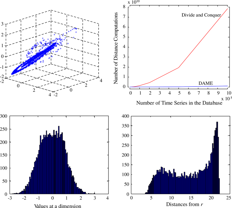
In this section, we show why it is a necessity to device a specialized algorithm that finds closest pair of subsequences termed as time series motifs. To facilitate that, we have placed our algorithm in the context of the divide and conquer methods for closest-pair which is prevalent in the text books of computational geometry. The divide and conquer (DaC) approach for finding closest pair in multidimensional space is described in great detail in Bentley (1980). DaC works in O(nlog^dn) time for any data distribution, which is expensive for large d. For “sparse” data DaC works in O(n log n). The relevant definition of sparsity is given “as the condition that no d-ball in the space (that is, a sphere of radius d) contains more than some constant c points. (Bentley 1980)” This condition ensures that the conquer step remains a linear operation with no more than cn pairs of close points to be compared. But subsequences of a long time series form a trail in the high dimensional space which may cross itself arbitrary number of times to violate the sparsity condition for efficient DaC algorithm [16]. A simple 3D demonstration is shown in Fig. 4 (top-left) by plotting all triplets of successive real numbers in an ECG time series.

Fig. 4.

(Top-left) Plot of successive triplets of numbers of a time series. (Top-right) Comparison of DAME with divide and conquer approach. (Bottom) Distribution of 10,000 random walks along (left) a plane perpendicular to an axis and (right) the order line

If we are only considering independent time series objects (c.f. sect. 6.4), it is still not a good choice to use DaC, because it divides the data by hyper planes perpendicular to an axis. This is because the range of the distribution of referenced distances (Fig. 4 bottom-right) is much larger than the range of possible values in a particular normalized dimension (Fig. 4 bottom-left). If the closest pair of time series has 95% correlation between them, the minimum Euclidian distance for m = 128 is 3.57. For this minimum distance, a perpendicular hyper plane through 0 would have all the points within [−3.57,3.57] and thus resulting in no pruning being achieved. In contrast, the reference point ordering has a larger range and can prune many pairs of points using the same bracket.

Considering the above two observations, we may expect DAME to perform much better than divide and conquer algorithm in Bentley (1980). As shown in Fig. 4 (top-right), this is the case. For a motif length of 128 we tested up to 1 million points of EEG time series and DaC performs 100 times more distance computations than DAME for the larger datasets. These results are in spite of the fact that we allowed DaC to “cheat”, by always using the best axis (the one that has minimum number of points within the bracket [−δ,δ]) to divide the data at each step.

5.2. Sanity check on large databases

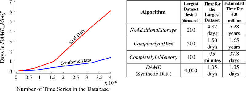
We begin with an experiment on random walk data. Random walk data is commonly used to evaluate time series algorithms, and it is an interesting contrast to the real data (considered below), since there is no reason to expect a particularly close motif to exist. We generate a database of four million random walks in eighty disk blocks. Each block is identical in size (400MB) and can store 50,000 random walks of length 1024. The database spans more than 32GB of hard drive space. We find the closest pair of random walks using DAME on the first 2, 4, 8, 16, 32, 64 and 80 blocks of this database. Figure 5 left shows the execution times against the database size in the number of random walks.

Fig. 5.

(Left) Execution times in days on random walks and EOG data. (Right) Comparison of the three different versions of brute-force algorithm with DAME

In another independent experiment we use DAME on a very long and highly oversampled real time series (EOG trace, cf. Sect. 6.5) to find a subsequence-motif of length 1024. We start with a segment of this long time series created by taking the first 100,000 data points, and iteratively double the segment-sizes by taking the first 0.2, 0.4, 0.8, 1.6, 3.2 and 4.0 million data points. For each of these segments, we run DAME with blocks of 400MBs, each containing 50,000 time series, as in the previous experiment. Figure 5: left also shows the execution times against the lengths of the segments. Because of the oversampled time series, the extra “noise” makes the motif distance larger than it otherwise would be, making the bsf larger and therefore reducing the effectiveness of pruning. This is why DAME takes longer to find a motif of the same length than in a random-walk database of similar size.

Since no other algorithm is reported to find motifs exactly on such large databases of such large dimensionalities, we have implemented three possible versions of the naïve brute force algorithm to compare with DAME:

• CompletelyInMemory: The database is in the main memory.

• CompletelyInDisk: The database is in the disk and memory is free enough to store only two disk blocks and negligible data structures for comparisons.

• NoAdditionalStorage: There is no database. Only the base time series is stored in the main memory. Subsequences must be normalized again and again every time they are extracted from the base time series.

Figure 5 right tabulates the performances of the above three algorithms as well as DAME’s. CompletelyInMemory algorithm has been run until memory allocation request is honored; therefore, estimated time for four million time series is unattainable, as it would need 32GB of main memory. The other two algorithms have been executed until time becomes critical. The estimated execution times demonstrates that DAME is the only tractable algorithm for exact discovery of time series motifs.

5.3. Performance for different block sizes

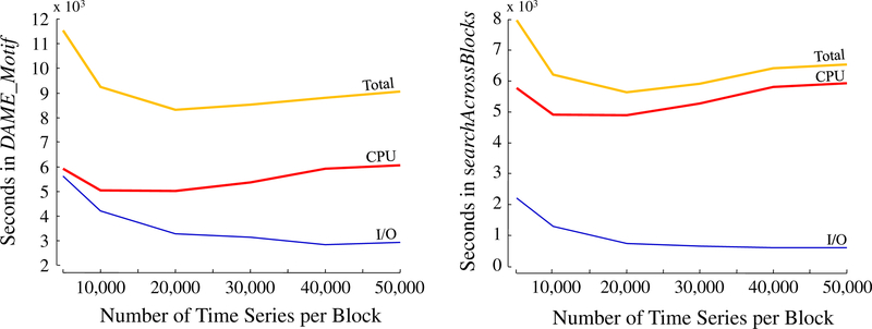
As DAME has a specific order of disk access, we must show how the performance varies with the size of the disk blocks. We have taken the first one million random walks from the previous section and created six databases with different block sizes. The sizes we test are 40, 80, 160, 240, 320 and 400MBs containing 5, 10, 20, 30, 40 and 50 thousands of random walks, respectively. Since the size of the blocks is changed, the number of blocks also changes to accommodate one million time series. We measure the time for both I/O and CPU separately for DAME_Motif (Fig. 6, left) and for searchAcrossBlocks (Fig. 6, right).

Fig. 6.

Total execution times with CPU and I/O components recorded on one million random walks for different block sizes (left) for the DAME_Motif method and (right) for the searchAcrossBlocks method

Figure 6 left shows that I/O time decreases as the size of the blocks gets larger and the number of blocks decreases. On the other hand, the CPU time is worse for very low or very high block sizes. Ideally it should be constant, as we use the same set of random walks. The two end deviations are caused by two effects: when blocks are smaller, block intervals become smaller compared to the closest pair distance, and therefore, almost every point is compared to points from multiple blocks and essentially istart loses its role. When the blocks become larger, consecutive pairs on the order line in later blocks are searched after the distant pairs on the order line in an earlier block. Therefore, bsf decreases at a slower rate for larger block sizes.

Figure 6 right shows that the search for a motif using the order line is a CPU-bound process since the gap between CPU time and I/O time is large, and any effort to minimize the number of disk loads by altering the loading order from the current sequential one will make little difference in the total execution time.

5.4. Performance for different motif lengths

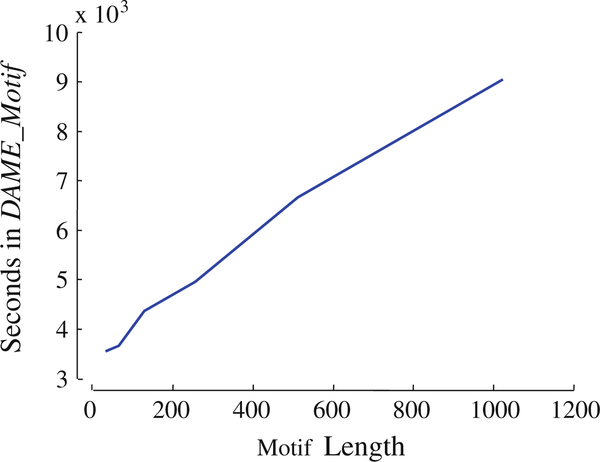
To explore the effect of the motif length (i.e. dimensionality) on performance, we test DAME for different motif lengths. Recall that the motif length is the only user-defined parameter. We use the first one-million random walks from Sect. 4.1. They are stored in 20 blocks of 50,000 random walks, each of length 1024. For this experiment, we iteratively double the motif length from 32 to 1024. For each length x, we use only the first x temporal points from every random walk in the database. Figure 7 shows the result, where all the points are averaged over five runs.

Fig. 7.

Execution times on one million random walks of different lengths

The linear plot demonstrates that DAME is free of any exponential constant (2^d) in the complexity expression, as in the optimal algorithm. The linear increase in time is due to the distance computation, which needs a complete scan of the data. Note the gentle slope indicating a sub-linear scaling factor. This is because longer motifs allow greater benefit from early abandoning (Mueen et al. 2009).

5.5. In-Memory search options

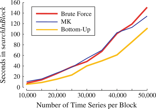
While searching within a memory block, DAME does a bottom-up search starting with pairs of consecutive time series, continuing until it covers all possible pairs. Thus, DAME has a consistent search hierarchy from within blocks to between blocks. There are only two other exact methods we could have used, the classic brute-force algorithm or the recently published MK algorithm (Mueen et al. 2009). We measure thetimethateachofthesemethodstakestosearchin-memoryblocksofdifferentsizes, and experiment on different sizes of blocks ranging from 10,000 to 50,000 random walks of length 1024. For all of the experiments, the databases are four times the block sizes and values are averaged over ten runs.

From the Fig. 8, brute force search and the MK algorithm perform similarly. The reason for MK not performing better than brute force here is worth considering. MK performs well when the database has a wide range and uniform variability on the order line. Since the database in this experiment is four times the block size, the range of distances for one block is about one fourth of what it would be in an independent one-block database of random walks. Therefore, MK cannot perform better than brute force. The bottom-up search performs best because it does not depend on the distribution of distances from the reference point, and moreover, prunes off a significant part of the distance computations.

Fig. 8.

Comparison of in-memory search methods

5.6. Lower bound options

In our algorithm we compute distances from r reference points to all of the objects. In the update method, we use each reference point one at a time to compute a lower bound on the distance between a pair and check to see if the lower bound is greater than the current best. This lower bound is a simple application of the triangular inequality computed by circularly projecting the pair of objects onto any line that goes through the participating reference point. We call this idea the “linear bound” for clarity in the following discussion. Since we pre-compute all of the distances from r reference points, one may think about getting a tighter lower bound by combining these referenced distances. In the simplest case, to find a “planar bound” for a pair of points using two reference points, we can project both the points (x and y) onto any 2D plane, where two reference points (r₁ and r₂) reside, by a circular motion about the axis connecting the reference points. After that, simple 2D geometry is needed to compute the lower bound (dashed line) using five other pre-computed distances (solid lines in Fig. 9, mid).

Fig. 9.

(Left) Two points x and y are projected on a plane by a rotation around the axis joining two reference points r₁ and r₂. (Mid) Known distances and the lower bound after the projection. (Right) Planar and linear bound are plotted against true distances for 40,000 random pairs

We have computed both the bounds on one million pairs of time series of length 256. In 56% of the pairs, planar bounds are larger than linear bounds. Intuitively it seems from this value that the planar bound is tighter. But the true picture is more complex. The average value of linear bounds is 30% larger than that of planar bounds and standard deviation of linear bounds is 37% larger than that of planar bounds. In Fig. 9 right, it is clear that the linear bound is significantly tighter than the planar one when the actual distances between pairs are larger. Moreover, the planar bound is complex to compute compared to a simple subtraction in the case of a linear bound. Therefore, we opt to use the linear bound in update to prune off distance computations.

6. Experimental case studies

In this section we consider several case studies to demonstrate the utility of motifs in solving real-world problems.

6.1. Motifs for brain–computer interfaces

Recent advances in computer technology make sufficient computing power readily available to collect data from a large number of scalp electroencephalographic (EEG) sensors and to perform sophisticated spatiotemporal signal processing in near-real time. A primary focus of recent work in this direction is to create brain–computer interface (BCI) systems.

In this case study, we apply motif analysis methods to data recorded during a target recognition EEG experiment (Bigdely-Shamlo et al. 2008). The goal of this experiment is to create a real-time EEG classification system that can detect “flickers of recognition” of the target in a rapid series of images and help Intelligence Analysts find targets of interest among a vast amount of satellite imagery. Each subject participates in two sessions: a training session in which EEG and behavior data are recorded to create a classifier and a test session in which EEG data is classified in real time to find targets. Only the training session data is discussed here.

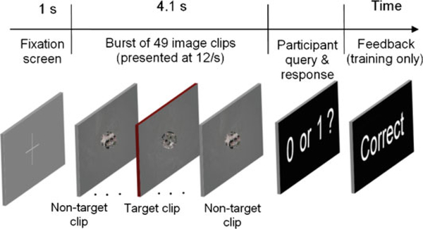
In this experiment, overlapping small image clips from a publicly available satellite image of London are shown to a subject in 4.1s bursts comprised of 49 images at the rate of 12 per second. Clear airplane targets are added to some of these clips such that each burst contains either zero (40%) or one (60%) target clip. To clearly distinguish target and non-target clips, only complete airplane target images are added, though they can appear anywhere and at any angle near the center of the clip.

Figure 10 shows a burst trial timeline. After fixating a cross (left) for 1s, the participant views the RSVP burst and is then asked to indicate whether or not he/she has detected a plane in the burst clips, by pressing one of two (yes/no) finger buttons.

Fig. 10.

A burst trial time line

In training sessions only, visual error/correct feedback is provided. The training session comprises of 504 RSVP bursts organized into 72 bouts with a self-paced break after each bout. In all, each session thus includes 290 target and 24,104 non-target image presentations. The EEG from 256 scalp electrodes at 256 Hz and manual responses are recorded during each session.

Each EEG electrode receives a linear combination of electric potentials generated from different sources in and outside the brain. To separate these signals, an extended-infomax Independent Component Analysis (ICA) algorithm (Lee et al. 1999; Delorme and Makeig 2003) is applied to preprocessed data from 127 electrodes to obtain about 127 maximally independent components (ICs). The ICA learns spatial filters in the form of an unmixing matrix separating EEG sensor data into temporally maximally independent processes, most appearing to predominantly represent the contribution to the scalp data of one brain EEG or non-brain artifact source, respectively.

It is known that among ICs representing brain signals, some show changes in activity after the subject detects a target. However, the exact relationships are currently unknown. In an ongoing project, we attempt to see if the occurrences of motifs are correlated with these changes.

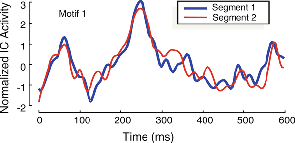
We use DAME to discover motif of length 600 ms (153 data points), on IC activity from 1s before until 1.5s after image presentation. Figure 11 shows the discovered motif.

Fig. 11.

Two subsequences corresponding to the first motif

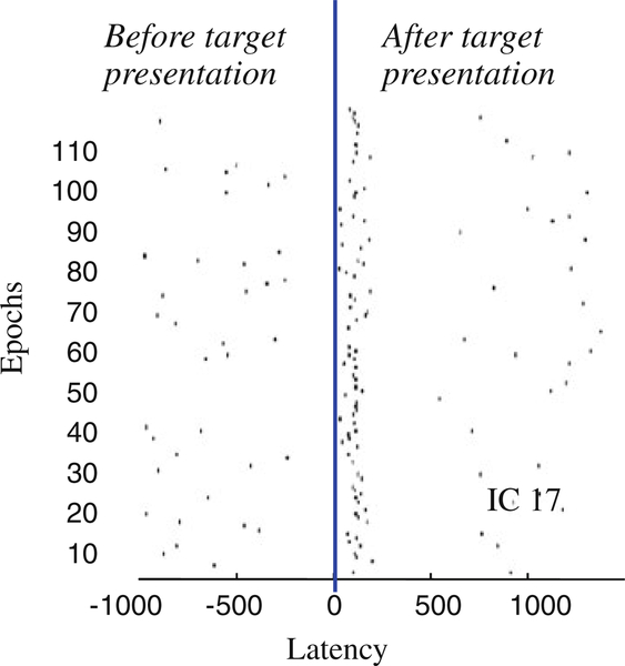
Figure 12 shows the start latencies of all of the 600ms segments which are within a distance of twice the motif distance (i.e. twice the Euclidean distance between the two time series shown in Fig. 11) from either of the motif segment. Note that the distribution of these latencies is highly concentrated around 100ms after target presentation (showed by the blue line). This is significant because no information about the latency of the target has been provided beforehand, and thus the algorithm finds a motif that is highly predictive of the latency of the target.

Fig. 12.

Motif 1 start latencies in epochs

6.2. Finding repeated insect behavior

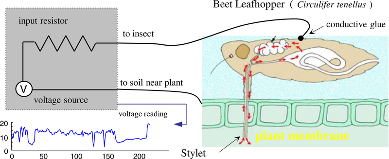
In the arid to semi-arid regions of North America, the Beet leafhopper (Circulifer tenellus) shown in Fig. 13, is the only known vector (carrier) of curly top virus, which causes major economic losses in a number of crops including sugarbeet, tomato, and beans (Kaffka et al. 2000). In order to mitigate these financial losses, entomologists at the University of California, Riverside are attempting to model and understand the behavior of this insect (Stafford and Walker 2009).

Fig. 13.

A schematic diagram showing the apparatus used to record insect behavior

It is known that the insects feed by sucking sap from living plants; much like the mosquito sucks blood from mammals and birds. In order to understand the insect’s behaviors, entomologists glue a thin wire to the insect’s back, complete the circuit through a host plant and then measure fluctuations in voltage level to create an Electrical Penetration Graph (EPG) as shown in Fig. 13.

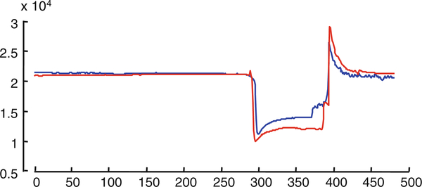
This method of data collection produces large amounts of data, in Fig. 14 we see about a quarter hour of data, however the entomologists data archive currently contains thousands of hours of such data, collected in a variety of conditions. Up to this point, the only analysis of this data has been some Fourier analyses, which has produced some suggestive results (Stafford and Walker 2009). However, Fourier analysis is somewhat indirect and removed from the raw data. In contrast motif discovery operates on the raw data itself and can potentiality produce more intuitive and useful knowledge. In Fig. 15 we show the motif of length 480 discovered in the entire 33,021 length time series shown in Fig. 14.

Fig. 14.

An electrical penetration graph of insect behavior. The data is complex and highly non-stationary, with wandering baseline, noise, dropouts, etc.

Fig. 15.

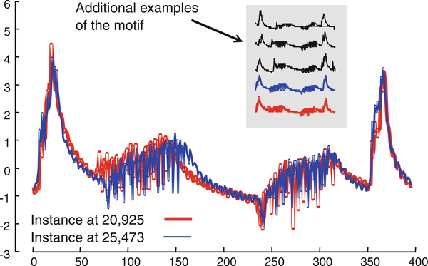
The motif of length 480 found in the insect telemetry shown in Fig. 14. Although the two instances occur minutes apart they are uncannily similar

As we can see, the motifs are uncannily similar, even though they occur minutes apart. Having discovered such a potentially interesting pattern, we followed up to see if it is really significant. The first thing to do is to see if it occurs in other datasets. We have indexed the entire archive with an iSAX index (Shieh and Keogh 2008) so we quickly determined the answer to be affirmative, this pattern does appear in many other datasets, although the “plateau” region(approximately from 300 to 380 in Fig. 15) may be linearly scaled by a small amount (Stafford and Walker 2009). We recorded the time of occurrence and looked at the companion video streams which were recorded synchronously with the EPGs. It appears that the motif occurs immediately after phloem (plant sap) ingestion has taken place.

The motif discovered in this stream happens to be usually smooth and highly structured, however motifs can be very complex and noisy. Consider Fig. 16 which shows a motif extracted from a different trace of length 18,667.

Fig. 16.

The motif of length 400 found in an EPG trace of length 18,667. (Inset) Using the motifs as templates, we can find several other occurrences in the same dataset

In this case, examination of the video suggests that this is a highly ritualized grooming behavior. In particular, the feeding insect must get rid of honeydew (a sticky secretion, which is by-product of sap feeding). As a bead of honeydew is ejected, it temporarily forms a highly conductive bridge between the insect and the plant, drastically affecting the signal.

Note that these examples are just a starting point for entomological research. It would be interesting to see if there are other motifs in the data. Having discovered such motifs we can label them, and then pose various hypotheses. For example: “Does motif A occur more frequently for males than females?” Furthermore, an understanding of which motifs correlate with which behaviors suggests further avenues for additional data collection and experiments. For example, it is widely believed that Beet leafhoppers are repelled by the presence of marigold plants(Tagetes).It may be possible touse the frequency of (now) known motifs to detect if there really is a difference between the behavior of insect with and without the presence of marigolds. We defer further discussion of such issues to future and ongoing work.

6.3. Automatically constructing EEG dictionaries

In this example of the utility of time series motifs we discuss an ongoing joint project between the authors and Physicians at Massachusetts General Hospital (MGH) in automatically constructing “dictionaries” of recurring patterns from electroencephalographs.

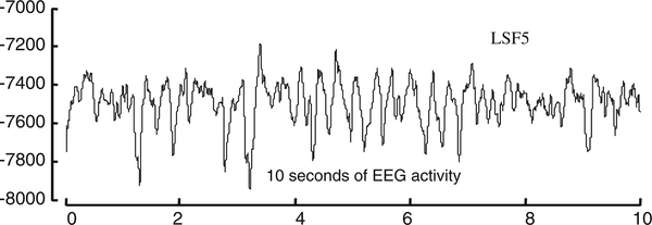
The electroencephalogram (EEG) measures voltage differences across the scalp and reflects the activity of large populations of neurons underlying the recording electrode (Niedermeyer and Lopes da Silva 1999). Figure 17 shows a sample snippet of EEG data.

Fig. 17.

The first 10s of an EEG trace. In the experiment discussed below, we consider a full hour of this data

Medical situations in which EEG plays an important role include, diagnosing and treating epilepsy; planning brain surgery for patients with intractable epilepsy, monitoring brain activity during cardiac surgery and in certain comatose patients; and distinguishing epileptic seizures from other medical conditions (e.g. “pseudoseizures”).

The interpretation of EEG data involves inferring information about the brain (e.g. presence and location of a brain lesion) or brain state (e.g. awake, sleeping, having a seizure) from various temporal and spatial patterns, or graphoelements (which we see as motifs), within the EEG data stream. Over the roughly 100 years since its invention in the early 1900s, electroencephalographers have identified a small collection of clinically meaningful motifs, including entities named “spike-and-wave complexes”, “wicket spikes”, “K-complexes”, “sleep spindles” and “alpha waves”, among many other examples. However, the full “dictionary” of motifs that comprise the EEG contains potentially many yet-undiscovered motifs. In addition, the current, known motifs have been determined based on subjective analysis rather than a principled search. A more complete knowledge of the full complement of EEG motifs may well lead to new insights into the structure of cortical activity in both normal circumstances and in pathological situations including epilepsy, dementia and coma.

Much of the recent research effort has focus on finding typical patterns that may be associated with various conditions and maladies. For example, (Stern and Engel 2004) attempts to be an “Atlas of EEG patterns”. However, thus far, all such attempts at finding typical patterns have been done manually and in an ad hoc fashion.

A major challenge for the automated discovery of EEG motifs is large data volumes. To see this, consider the following experiment. We conducted a search for the motif of length 4s, within a 1h EEG from a single channel in a sleeping patient. The data collection rate was 500 Hz, yielding approximately 2 million data points, after domain standard smoothing and filtering, an 180,000 data point signal was produced. Using the brute force algorithm in the raw data, finding the motif required over 24h of CPU time. By contrast, using the in memory version of the algorithm described in this paper, the same result requires 2.1min, a speedup of about factor of about 700. Such improvements in processing speed are crucial for tackling the high data volume involved in large-scale EEG analysis. This is especially the case in attempting to complete a dictionary of EEG motifs which incorporates multi-channel data and a wide variety of normal situations and disease states.

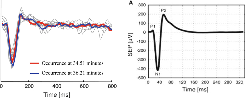
Having shown that automatic exploration of large EEG datasets is tractable, our attention turns to the question, is it useful? Figure 18 left shows the result of our first run of our algorithm and Fig. 18 right shows a pattern discussed in a recent paper (Stefanovic et al. 2007).

Fig. 18.

(Left) Bold lines the first motif found in one hour of EEG trace LSF5. Light lines the ten nearest neighbors to the motif. (Right) A screen dump of Fig. 6, from paper Stefanovic et al. (2007)

It appears that this automatically detected motif corresponds to a well-known pattern, the K-complex. K-complexes were identified in 1938 (Niedermeyer and Lopes da Silva 1999; Loomis et al. 1938) as a characteristic event during the sleep.

This figure is at least highly suggestive that in this domain, motif discovery can really find patterns that are of interest to the medical community. In ongoing work we are attempting to see if there are currently unknown patterns hiding in the data.

6.4. Detecting near-duplicate images

Finding near-duplicate images in an image database can be used to summarize the database, identify forged images and clean out distorted copies of images. If we can convert the two-dimensional ordered images into one-dimensional (possibly unordered) vectors of features, we can use our motif discovery algorithm to find near-duplicate images.

To test this idea, we use the first 40 million images from the dataset in Torralba et al. (2008). We convert each image to a pseudo time series by concatenating its normalized color histograms for the three primary colors (Hafner and Sawhney 1995). Thus, the lengths of the “time series” are exactly 768. We run DAME on this large set of time series and find 1,719,443 images which have at least one and on average 1.231 duplicates in the same dataset. We also find 542,603 motif images which have at least one non-identical image within 0.1 Euclidean distances of them. For this experiment, DAME has taken 6.5 days (recall that a brute-force search would take over a century, cf. Sect. 5). In Fig. 19, samples from the sets of duplicates and motifs are shown. Subtle differences in the motif pairs can be seen; for example, a small “dot” is present next to the dog’s leg in one image but not in the other. The numbers in between image pairs are the ids of the images in the database.

Fig. 19.

(Left) Five identical pairs of images. (Right) Five very similar, but non-identical pairs

6.5. Discovering patterns in polysomnograms

In polysomnography, body functions such as pulse rate, brain activity, eye movement, muscle activity, heart rhythm, breathing, etc. are monitored during a patient’s sleep cycle. To measure the eye movements an Electrooculogram (EOG) is used. Eye movements do not have any periodic pattern like other physiological measures such as an ECG and respiration. Repeated patterns in the EOG of a sleeping person have attracted much interest in the past because of their potential relation to dream states. We use DAME to find a repeated pattern in the EOG traces from the “Sleep Heart Health Study Polysomnography Database” (Goldberger et al. 2000). The trace has about 8,099,500 temporal values at the rate of 250 samples per second. Since the data is oversampled, we downsample it to a time series of 1,012,437 points. A subset of 64s is shown in Fig. 20.

Fig. 20.

A section of the EOG from the polysomnogram traces

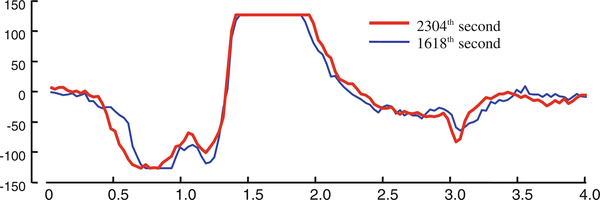
After a quick review of the data, one can identify that most of the natural patterns are shorter in length (i.e. 1 or 2 s) and are visually detectable locally in a single frame. Instead of looking for such shorter patterns, we search for longer patterns of 4.0s long with the hope of finding visually undetectable and less frequent patterns. DAME has finished the search in 10.5h (brute force search would take an estimated 3 months) and found two subsequences shown in Fig. 21 which have a common pattern, and very unusually this pattern does not appear anywhere else in the trace. Note that the pattern has a plateau in between seconds 1.5 and 2.0, which might be the maximum possible measurement by the EOG machine.

Fig. 21.

Motif of length 4.0 s found in the EOG

We map these two patterns back to the annotated dataset. Both the subsequences are located at points in the trace just as the person being monitored was going back and forth between arousal and sleep stage 1, which suggests some significance to this pattern.

6.6. Extension to multidimensional motifs

Because DAME works with any metric distance measure, it is very easily extendible to multidimensional time series, so long as we use a metric to measure distances among them. We can use multidimensional Euclidean distance for multidimensional time series which is computed by taking the Euclidean distance for all the values along each of the dimensions. The squared errors from different dimensions can be weighted by their relative importance. Any weighting scheme preserves the metric property of Euclidean distance and thus our algorithm is directly applicable to multidimensional data.

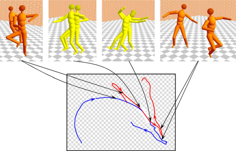
A good example of multidimensional time series is human motion capture data where the 3D positions and angles of several joints of the body are recorded while a subject performs a specific motion. The positions of different joints are synchronous time series and can be considered as different dimensions of a multidimensional time series. While computing the similarity of motion segments, we must define the relative importance (weights) of different body parts. For example, to compare Indian dances we may need to put larger weights on the hands and legs than head and chest. To test the applicability of DAME on multidimensional data, we use two dance motions from the CMU motion capture databases and identified the motion-motif shown in Fig. 22. Each of the dance motions are more than 20s long and we search for motif of length 1s. The motion-motif we found is a dance segment that denotes “joy” in Indian dance.

Fig. 22.

An example of multidimensional motif found in the motion captures of two different Indian dances. In the top row, four snapshots of the motions aligned at the motif are shown. In the bottom, the top-view of the dance floor is shown and the arrows show the positions of the subjects

7. Conclusion and future work

In this paper we introduced the first scalable algorithm for exact discovery of time series motif. Our algorithm can handle databases of the order of tens of millions of time series, which is at least two orders of magnitude larger than anything attempted before. We used our algorithm in various domains and discovered significant motifs. To facilitate scalability to the handful of domains that are larger than those considered here (i.e. star light curve catalogs), we plan to consider parallelization, given that the search for different group sizes can easily be delegated to different processors. Another avenue of research is to modify the algorithm to find multidimensional motifs in databases of similar scale.

References

- Abe H, Yamaguchi T (2005) Implementing an integrated time-series data mining environment—a case study of medical Kdd on chronic hepatitis. In: Presented at the 1st international conference on complex medical engineering (CME2005) [Google Scholar]
- Androulakis I, Wu J, Vitolo J, Roth C (2005) Selecting maximally informative genes to enable temporal expression profiling analysis, In: Proceddings of foundations of systems biology in engineering [Google Scholar]
- Arita D, Yoshimatsu H, Taniguchi R (2005) Frequent motion pattern extraction for motion recognition in real-time human proxy. In: Proceedings of JSAI workshop on conversational informatics, pp 25–30 [Google Scholar]
- Beaudoin P, Van de Panne M, Poulin P, Coros S (2008) Motion-motif graphs, symposium on computer animation [Google Scholar]
- Bentley JL (1980) Multidimensional divide-and-conquer. Commun ACM 23(4):214–229 [Google Scholar]
- Bigdely-Shamlo N, Vankov A, Ramirez R, Makeig S (2008) Brain activity-based image classification from rapid serial visual presentation. IEEE Trans Neural Syst Rehabil Eng 16(4) [DOI] [PubMed] [Google Scholar]
- Böhm C, Krebs F (2002) High performance data mining using the nearest neighbor join. In: Proceedings of 2nd IEEE international conference on data mining (ICDM), pp 43–50 [Google Scholar]
- Celly B, Zordan V (2004) Animated people textures. In: Proceedings of 17th international conference on computer animation and social agents (CASA) [Google Scholar]
- Cheung SS, Nguyen TP (2005) Mining arbitrary-length repeated patterns in television broadcast. ICIP 3:181–184 [Google Scholar]
- Chiu B, Keogh E, Lonardi S (2003) Probabilistic discovery of time series motifs. In: ACM SIGKDD, Washington, DC, pp 493–498 [Google Scholar]
- Corral A, Manolopoulos Y, Theodoridis Y, Vassilakopoulos M (2000) Closest pair queries in spatial databases. In: SIGMOD [Google Scholar]
- Delorme A, Makeig S (2003) EEG changes accompanying learning regulation of the 12-Hz EEG activity. IEEE Trans Rehabil Eng 11(2):133–136 [DOI] [PubMed] [Google Scholar]
- Ding H, Trajcevski G, Scheuermann P, Wang X, Keogh E (2008) Querying and mining of time series data: experimental comparison of representations and distance measures. In: VLDB [Google Scholar]
- Dohnal V, Gennaro C, Zezula P (2003) Similarity join in metric spaces using eD-Index, vol 2736 In: DEXA, pp 484–493 [Google Scholar]
- Duchêne F, Garbay C, Rialle V (2007) Learning recurrent behaviors from heterogeneous multivariate time-series. Artif Intell Med 39(1):25–47 [DOI] [PubMed] [Google Scholar]
- Faloutsos C, Ranganathan M, Manolopoulos Y (1994) Fast subsequence matching in time-series databases. In: SIGMOD, pp 419–429 [Google Scholar]
- Ferreira P, Azevedo PJ, Silva C, Brito R (2006) Mining approximate motifs in time series. Discov Sci [Google Scholar]
- Goldberger AL, Amaral LAN, Glass L, Hausdorff JM, Ivanov PCh, Mark RG, Mietus JE, Moody GB, Peng C-K, Stanley HE (2000) PhysioBank, physiotoolkit, and physionet: components of a new research resource for complex physiologic signals. Circulation 101(23):e215–e220 [DOI] [PubMed] [Google Scholar]
- Gonzalez EC, Figueroa K, Navarro G (2008) Effective proximity retrieval by ordering permutations. IEEE Trans Pattern Anal Mach Intell 30(9):1647–1658 [DOI] [PubMed] [Google Scholar]
- Guyet T, Garbay C, Dojat M (2007) Knowledge construction from time series data using a collaborative exploration system. J Biomed Inform 40(6):672–687 [DOI] [PubMed] [Google Scholar]
- Hafner J, Sawhney H et al. (1995) Efficient color histogram indexing for quadratic form distance functions. IEEE Trans Pattern Anal Mach Intell 17(7):729–736 [Google Scholar]
- Hamid R, Maddi S, Johnson A, Bobick A, Essa I, Isbell C (2005) Unsupervised activity discovery and characterization from event-streams. In: Proceedings of the 21st conference on uncertainty in artificial intelligence (UAI05) [Google Scholar]
- Jagadish HV, Ooi BC, Tan K, Yu C, Zhang R (2005) iDistance: An adaptive B+-tree based indexing method for nearest neighbor search. ACM Trans Database Syst 30(2) [Google Scholar]
- Kaffka S, Wintermantel B, Burk M, Peterson G (2000) Protecting high-yielding sugarbeet varieties from loss to curly top. http://sugarbeet.ucdavis.edu/Notes/Nov00a.htm
- Keogh EJ (2003) Efficiently finding arbitrarily scaled patterns in massive time series databases. In: Proceedings of the 7th European conference on principles and practice of knowledge discovery in databases (PKDD), pp 253–265 [Google Scholar]
- Keogh EJ, Wei L, Xi X, Lee S-H, Vlachos M (2006) LB_Keogh supports exact indexing of shapes under rotation invariance with arbitrary representations and distance measures. In: VLDB, pp 882–893 [Google Scholar]
- Koudas N, Sevcik KC (2000) High dimensional similarity joins: algorithms and performance evaluation. IEEE Trans Knowl Data Eng 12(1):3–18 [Google Scholar]
- Lee T, Girolami M, Sejnowski TJ (1999) Independent component analysis using an extended infomax algorithm for mixed subgaussian and supergaussian sources. Neural Comput 11(2):417–441 [DOI] [PubMed] [Google Scholar]
- Lin J, Keogh E, Lonardi S, Patel P (2002) Finding motifs in time series. In: 2nd workshop on temporal data mining (KDD’02) [Google Scholar]
- Liu Z, YU JX, Lin X, Lu H, Wang W (2005) Locating motifs in time-series data. In: PAKDD, pp 343–353 [Google Scholar]
- Loomis AL, Harvey E, Hobart G (1938) Disturbance patterns in sleep. J Neurophysiol 2:413–430 [Google Scholar]
- McGovern A, Rosendahl D, Kruger A, Beaton M, Brown R, Droegemeier K (2007) Understanding the formation of tornadoes through data mining. In: 5th conference on artificial intelligence and its applications to environmental sciences at the American meteorological society [Google Scholar]
- Meng J, Yuan J, Hans M, Wu Y (2008) Mining motifs from human motion. In: Proceedings of EUROGRAPHICS [Google Scholar]
- Minnen D, Isbell CL, Essa I, Starner T (2007a) Detecting subdimensional motifs: an efficient algorithm for generalized multivariate pattern discovery. In: IEEE ICDM [Google Scholar]
- Minnen D, Isbell CL, Essa I, Starner T (2007b) Discovering multivariate motifs using subsequence density estimation and greedy mixture learning. In: 22nd conference on artificial intelligence [Google Scholar]
- Motzkin D, Hansen CL (1982) An efficient external sorting with minimal space requirement. Int J Parallel Program 11(6):381–396 [Google Scholar]
- Mueen A, Keogh E, Zhu Q, Cash S, Westover B (2009) Exact discovery of time series motif. In: SDM; [DOI] [PMC free article] [PubMed] [Google Scholar]
- Murakami K, Doki S, Okuma S, Yano Y (2005) A study of extraction method of motion patterns observed frequently from time-series posture data. In: Proceedings of IEEE international conference on systems, man and cybernetics (SMC), pp 3610–3615 [Google Scholar]
- Nanopoulos A, Theodoridis Y, Manolopoulos Y (2001) C2P: clustering based on closest pairs. In: International conference on very large data bases (VLDB), pp 331–340 [Google Scholar]
- Niedermeyer E, Lopes da Silva F (eds) (1999) Electroencephalography: basic principles, clinical applications and related fields. Williams and Wilkins, Baltimore [Google Scholar]
- Nyberg C, Barclay T, Cvetanovic Z, Gray J, Lomet D (1995) Alphasort: A cache-sensitive parallel external sort. VLDB J 4(4):603–628 [Google Scholar]
- Patel P, Keogh E, Lin J, Lonardi S (2002) Mining motifs in massive time series databases. In: IEEE international conference on data mining [Google Scholar]
- Rombo S, Terracina G (2004) Discovering representative models in large time series databases. In: Proceedings of the 6th international conference on flexible query answering systems, pp 84–97 [Google Scholar]
- Shieh J, Keogh E (2008) iSAX: Indexing and mining terabyte sized time series. In: IGKDD, pp 623–631 [Google Scholar]
- Simona R, Giorgio T (2004) Discovering representative models in large time series databases. Int Conf Query Answ Syst 3055:84–97 [Google Scholar]
- Stafford C, Walker G (2009) Characterization and correlation of DC electrical penetration graph waveforms with feeding behavior of beet leafhopper (submission) [Google Scholar]
- Stefanovic BJ, Schwindt W, Hoehn M, Silva AC (2007) Functional uncoupling of hemodynamic from neuronal response by inhibition of neuronal nitric oxide synthase. J Cereb Blood Flow Metab 27:741–754 [DOI] [PubMed] [Google Scholar]
- Stern JM, Engel J Jr (2004) Atlas of EEG patterns. Williams & Wilkins, Lippincott Supporting Webpage www.cs.ucr.edu/~mueen/DAME/index.html [Google Scholar]
- Tanaka Y, Iwamoto K, Uehara K (2005) Discovery of time-series motif from multi-dimensional data based on MDL principle. Mach Learn 58(2–3):269–300 [Google Scholar]
- Tang H, Liao SS (2008) Discovering original motifs with different lengths from time series source. Knowl-Based Syst 21(7):666–671 [Google Scholar]
- Tata S (2007) Declarative querying for biological sequences, Ph.D Thesis, The University of Michigan, (Advisor Patel Jignesh M.) [Google Scholar]
- Torralba A, Fergus R, Freeman WT (2008) 80 million tiny images: a large database for non-parametric object and scene recognition. IEEE PAMI 30(11):1958–1970 [DOI] [PubMed] [Google Scholar]
- Ueno K, Xi X, Keogh E, Lee D (2006) Anytime classification using the nearest neighbor algorithm with applications to stream mining. In: Proceedings of of IEEE international conference on data mining (ICDM) [Google Scholar]
- Weber R, Schek H-J, Blott S (1998) A quantitative analysis and performance study for similarity-search methods in high-dimensional spaces. In: International conference on very large data bases (VLDB), pp 194–205 [Google Scholar]
- Wilson DR, Martinez TR (2000) Reduction techniques for instance-based learning algorithms machine learning, vol 38 Kluwer, Dordrecht, pp 257–286 [Google Scholar]
- Yankov D, Keogh E, Medina J, Chiu B, Zordan B (2007) Detecting motifs under uniform scaling. In: SIGKDD [Google Scholar]
- Yoshiki T, Kazuhisa I, Kuniaki U (2005) Discovery of time-series motif from multi-dimensional data based on MDL principle. Mach Learn 58(2–3):269–300 [Google Scholar]
- Yu C, Wang S (2007) Efficient index-based KNN join processing for high-dimensional data. Inf Softw Technol 49(4) [Google Scholar]