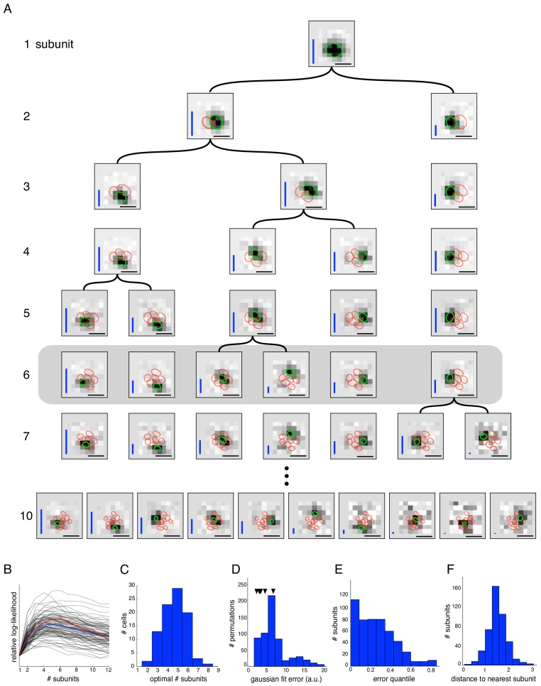
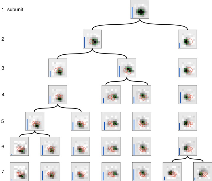
Figure 2. Estimated subunit properties.
(A) Subunits, shown as grayscale images, estimated from OFF parasol cell responses to 24 min of white noise. Each pixel was temporally prefiltered with a kernel derived from the spike-triggered average (STA). Rows show estimated spatial subunits for successive values of N. Subunit locations are indicated with ellipses (green for same subunit, red for other subunits from the same fit), corresponding to the contour of a fitted two-dimensional Gaussian with standard deviation equal to the average nearest neighbor separation between subunits. As N increases, each successive set of subunits may be (approximately) described as resulting from splitting one subunit into two (indicated by lines). Large N (e.g. last row) yields some subunits that are noisy or overlap substantially with each other. Height of vertical blue bars indicate the relative strength (average contribution to the cell's firing rate over stimulus ensemble, ignoring the output nonlinearity) of each subunit (see Equation 6 in Materials and methods). Horizontal black bars indicate spatial scale (150μm). (B) Log-likelihood as a function of number of subunits (relative to single subunit model) for 91 OFF parasol cells (black) on 3 min of held-out test data, averaged across 10 random initializations of the model, from a distinct randomly sampled training data (24 min from remaining 27 min of data). Population average is shown in blue and the example cell from (A) is shown in red. (C) Distribution of optimal number of subunits across different cells, as determined by cross-validated log-likelihood on a held-out test set for OFF parasol cells. (D, E) Spatial locality of OFF parasol subunits, as measured by mean-squared error of 2D gaussian fits to subunits after normalizing with the maximum weight over space. Control subunits are generated by randomly permuting pixel weights for different subunits within a cell. For this analysis, the optimal number of subunits was chosen for each cell. (D) Distribution of MSE values for randomly permuted subunits for the cell shown in (A). MSE of six (optimal N) estimated subunits indicated with black arrows. (E) Distribution of quantiles of estimated OFF parasol subunits, relative to the distribution of MSE values for permuted subunits, across all cells and subunits. Null hypothesis has uniform distribution between 0–1. (F) Distribution of distances to nearest neighboring subunit within each OFF parasol cell. Distances are normalized by geometric mean of standard deviation of the gaussian fits along the line joining center of subunits. For this analysis, each cell is fit with five subunits (most frequent optimum from (C)).


