

Abstract
Characterizing functional brain connectivity using resting functional magnetic resonance imaging (fMRI) is challenging due to the relatively small Blood-Oxygen-Level Dependent contrast and low signal-to-noise ratio. Denoising using surface-based Laplace-Beltrami (LB) or volumetric Gaussian filtering tends to blur boundaries between different functional areas. To overcome this issue, a time-based Non-Local Means (tNLM) filtering method was previously developed to denoise fMRI data while preserving spatial structure. The kernel and parameters that define the tNLM filter need to be optimized for each application. Here we present a novel Global PDF-based tNLM filtering (GPDF) algorithm that uses a data-driven kernel function based on a Bayes factor to optimize filtering for spatial delineation of functional connectivity in resting fMRI data. We demonstrate its performance relative to Gaussian spatial filtering and the original tNLM filtering via simulations. We also compare the effects of GPDF filtering against LB filtering using individual in-vivo resting fMRI datasets. Our results show that LB filtering tends to blur signals across boundaries between adjacent functional regions. In contrast, GPDF filtering enables improved noise reduction without blurring adjacent functional regions. These results indicate that GPDF may be a useful preprocessing tool for analyses of brain connectivity and network topology in individual fMRI recordings.
Keywords: Connectivity, fMRI, Non-local Means Filtering, Optimization
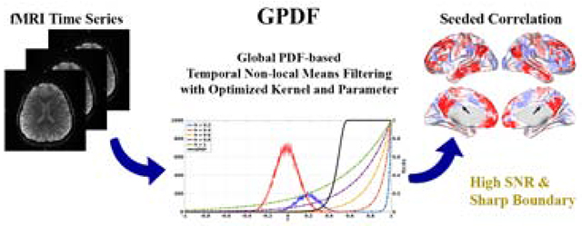
Graphical Abstract
1. Introduction
Functional MRI (fMRI) is a powerful in-vivo neuroimaging modality that allows us to indirectly infer information about the neuronal activity of the brain by measuring Blood-Oxygen-Level Dependent (BOLD) signal fluctuations (Ogawa et al., 1990). Temporal correlations in resting fMRI (rfMRI) BOLD signals across multiple spatially distinct brain areas are often used to define functional brain networks (Smith et al., 2009). However, BOLD signals inherently have low signal-to-noise ratio (SNR). Preprocessing of fMRI data often includes a spatial smoothing step to reduce noise. Isotropic 3D Gaussian filtering is the most commonly used approach to smooth volumetric rfMRI data (Smith et al., 2013), or equivalently, Laplace Beltrami (LB) smoothing is applied when the data is mapped onto a 2D representation of the cortical surface (Angenent, 1999). Both methods suffer from a critical common problem: they spatially mix signals along the borders between adjacent functional regions (Bhushan et al., 2016), limiting our ability to accurately identify connectivity at the micro-to-meso scale in individual fMRI recordings.
Non-local means (NLM) filtering is an edge-preserving method originally designed for natural image denoising (Buades et al., 2005) and more recently adapted for anatomical MRI (Manjon et al., 2008; Coupe et al., 2008), fMRI (Bernier et al., 2014) and diffusion MRI (Wiest-Daessle et al., 2008) to preserve spatial structure in imaging data. We recently developed a variant for filtering rfMRI data called temporal NLM (tNLM) that assigns non-local smoothing kernel weights based on temporal similarities between time series rather than spatial similarities (Bhushan et al., 2016). We demonstrated tNLM filtering’s ability to reduce noise by using (weighted) averages of only those times series that are similar, thus minimizing blurring across functional boundaries.
Here we identify two key challenges in using tNLM filtering as described in Bhushan et al. (2016). First, the exponential kernel function used in computing the weights is chosen heuristically. The exponent is an affine function of the sample correlation between the two time-series. As we show below, this function does not perform well in terms of optimizing the trade-off between the application of large weights when the correlations are high and smaller (or near zero) weights for low correlations. A second issue is that almost all NLM-based filtering methods, including tNLM, have been applied over a restricted neighborhood around the point to be filtered, partially because of the high computational cost if they are applied globally. However, since networks span the entire brain, global rather than local filtering has the potential for improved results when filtering using tNLM. It has been suggested previously that the brain has the structure of a small-world network (Bullmore and Sporns, 2009) and therefore most “nodes” (or voxels) in the brain are not strongly correlated with each other. As a result, when filtering a particular node using data from the entire brain, the fraction of uncorrelated nodes is much larger than the portion of correlated nodes. This can result in an undue influence of uncorrelated nodes if the filter weights applied to these nodes are not sufficiently suppressed. We address each of these issues in the methods described below.
Here we propose Global PDF-based tNLM filtering (GPDF): a new kernel function for tNLM filtering of fMRI data based on the probability density function (PDF) of the correlation of the time series between pairs of voxels. This method enables us to perform global filtering with improved noise reduction while minimizing blurring of adjacent functional regions.
An outline and some preliminary results of the approach described here have been previously reported (Li et al., 2018). The current paper provides a more detailed description of the method and novel experimental results to demonstrate its performance.
2. Method
2.1. NLM-based Filtering and tNLM
Let’s assume the fMRI data are represented on a 2D tessellation of the mid-cortical surface with V vertices and T time samples for each vertex. Let s(i, t) be the time series at vertex i ∈ V and time t ∈ T. Let Si be the set of vertices that are used to compute the filtered signal at vertex i. In the tNLM method, Si contains vertex i and all its k-hop neighboring vertices, for some k > 0. Then tNLM filtering is defined as
| (1) |
where the weight w(i, j) is chosen to be a temporal similarity measure and defined as a function of the sample correlation (Bhushan et al., 2016):
| (2) |
| (3) |
where r(i, j) is the Pearson correlation coefficient between vertices i and j and h is the parameter that controls the degree of filtering.
2.2. Global PDF-based tNLM Filtering
GPDF filtering differs from tNLM in the following two ways: (i) the spatial range over which the filtered signal is computed: in GPDF the set S i = S , ∀i, where S contains all vertices on the tessellated brain surface instead of just a local neighborhood; (ii) we use a different kernel function f in Equation (2).
2.2.1. GPDF Kernel Formulation
Let the observed signal be xi = si + ni at vertex i, a superposition of the true signal si and noise ni. Assume that si and ni are independent with and . Also assume some non-zero correlation between si and sj if i and j are within the same functional network (H1) and zero correlation if they are in different networks (H0). Then the correlation between two observed signals is:
| (4) |
where c ∈ [−1, 0) ∪ (0, 1] represents some non-zero correlation between true signals and represents the standard deviation (SD) of xi. If we let be the SNR-dependent scalar in Equation (4) under H1, then ρij = Kc. Therefore, ρij → 0 when K → 0 (low SNR case) and ρij → c when K → 1 (high SNR case). To further help avoid numerical issues and improve the robustness of the algorithm described below, we formulate our hypothesis in a slightly relaxed form:
| (5) |
where δ is a small positive constant. The sample correlation distribution is given by the following (Fisher, 1915):
| (6) |
where T is the number of samples and 2F1(a, b; c; z) is the Gaussian hypergeometric function. The parameter T will be omitted in the following derivation as for a given fMRI dataset, T is a fixed constant.
An example is shown in Fig. 1 where ρ = 0.2 under H1 (blue curve) and ρ = 0 under H0 (red curve). The histograms of the sample correlations are distributed about their means according to Equation (6) due to the finite number of samples. This causes a significant overlap between the red and blue curves. There is therefore a range of nonzero correlation values over which it is difficult to distinguish H1 from H0 given an observed sample correlation r. But to perform well, tNLM should attach large weights only to those time series for which H1 is true.
Figure 1:
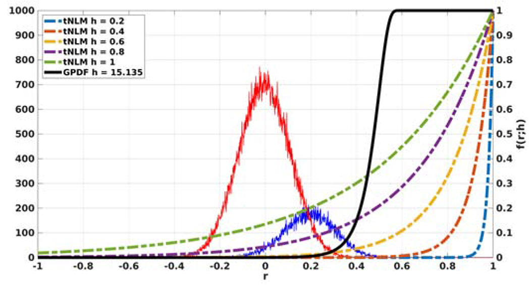
Histograms of the correlations under H1 (blue) and H0 (red) generated from simulated data overlaid with tNLM kernel functions for different parameter h (dotted) and GPDF kernel function with optimized parameter h (black solid).
In Fig. 1, we show the shape of the original tNLM kernel defined in Equation (3) as a function of h (dotted color curves). The figure shows that the kernel performs a poor job in differentiating H1 from H0 in the sense that applying significant weights for H1 also results in weights significantly greater than zero for H0. The black curve shows an alternative kernel that, visually at least, does a better job of giving significantly larger weights to H1 while minimizing those for H0. We now describe how we select this kernel and then evaluate its performance.
Bayes theorem tells us the posterior probability of ρ given r is
| (7) |
To better differentiate H1 from H0, we take the ratio between the integrated posterior probability under H1 and the counterpart under H0 (using the estimated priors described below), forming the Bayes factor (Kass and Raftery, 1995)
| (8) |
where R(r) ∈ [0, ∞). The larger R(r), the more likely ρ belongs to H1 given that sample correlation r. The constant δ, which separates H1 from H0 in Equation (5), was chosen such that the center area under the theoretical null hypothesis distribution is approximately 0.5, i.e., , for both the simulation and the real data experiments below.
We then reformulate our kernel function f to be
| (9) |
where, similar to the tNLM kernel in Equation (3), h is a parameter that controls the degree of smoothing. Replacing the sample correlation in Equation (3) with the Bayes factor in Equation (8) introduces the strong nonlinearity visible in the black curve in Fig. 1. This nonlinearity accounts for the fact that the posterior probability of H1 vs H0 can change rapidly as a function of r, as reflected in the Bayes factors.
2.2.2. Automated Parameter Selection
In addition to using a different kernel, we also propose an automated method for selecting the parameter h. An optimized parameter h for tNLM filtering is crucial because (i) the filtering effect is very sensitive to the selection of h as shown in Li and Leahy (2017); (ii) GPDF filtering uses a data-dependent kernel so that the parameters can vary substantially as different scanning protocols may have different time series duration and physiological noise sensitivity. Let be the marginal probability of r under H1 (using the estimated prior described below) and PH0(r) similarly defined under H0. To select the best parameter, we maximize the expected value of the weighting function fGPDF(r; h) with respect to PH1(r) while controlling the mean value with respect to PH0(r). Specifically,
| (10) |
where , i = 0, 1 and α is the expected weight under H0, analogous to the false positive rate in detection theory. Although α is another parameter we need to tune manually, it is more meaningful and robust than h, because choosing the same α will generally yield similar filtering results across different datasets while the internal parameter h can have a very different impact as a function of the noise level, range of correlation values and size of the image being filtered. We recommend that α be set conservatively, e.g. 10−3 or smaller, due to the dominant fraction of uncorrelated vertices (H0) in an fMRI dataset.
2.2.3. Estimation of the Population Correlation Distribution
In order to construct the kernel function in Equation (9) we need to know the Bayes factor R(r) in Equation (8), which requires the conditional distribution P(r|ρ) and the population correlation distribution PHi(ρ), i = 0, 1. The sample correlation density P(r|ρ) has the analytical solution given in Equation (6). Therefore, we need only estimate PHi(ρ), i = 0, 1. According to Equation (5), we assume no overlap between PH1(ρ) and PH0(ρ), i.e., PH1(ρ) = 0 for ρ ∈ [−δ, δ] and PH0(ρ) = 0 for ρ ∈ [−1, −δ) ∪ (δ, 1]. Let P(ρ) = PH1(ρ) + PH0(ρ) and P(r) be the empirical sample correlation distribution obtained from the fMRI data. Let and be the discretized version of the corresponding variables in the continuous space, respectively. Then PH1(ρ) and PH0(ρ) can be jointly estimated using a linear regression with non-negativity constraints:
| (11) |
This optimization is a well-posed problem as long as M ≥ N, i.e., the discretization step for r is smaller than that for ρ, which can be achieved easily. Our choice of step size of 0.001 for r and 0.01 for ρ results in stable estimates in all simulation and real data experiments below. Also, this problem can be solved efficiently using the fast non-negative least squares method (Bro and De Jong, 1997). Finally, and can be obtained as follows:
| (12) |
2.2.4. GPDF Filtering Algorithm
We summarize GPDF filtering algorithm as follows:
Algorithm I.
GPDF filtering
| 1: | Given fMRI data , calculate the correlation matrix |
| 2: | Estimate P′(r) from the histogram of the elements of A |
| 3: | Estimate the priors by solving Equation (11) |
| 4: | Compute the Bayes factor in Equation (8) |
| 5: | Optimize the parameter h by solving Equation (10) |
| 6: | Construct the kernel using Equation (9) |
| 7: | Finally filter the signal using Equation (1) |
Note that although the GPDF algorithm is presented and derived using data represented on a 2D tessellated surface, it can be generalized to any time series data, such as 3D volumetric fMRI data or a mix of surface and volumetric data (e.g. the grayordinate representations used in the Human Connectome Project (HCP) (Van Essen et al., 2013) dataset).
3. Experiments and Results
3.1. Simulation
We simulated a “brain surface” tessellation as two 2D blocks of size V × V (V = 32) representing left and right hemispheres. Each point in each block represents a vertex on the brain surface and has a label indicating which network it belongs to. Figure 2 (a) shows the ground truth label blocks where each color represents a distinct network. The top and bottom rows have identical labels to simulate connections between the left and right hemispheres (in total K = 16 unique labels). For each label, we generated a random time series (white noise) of length T = 200 where points within the same labels were given identical time series (perfectly correlated) in the absence of additional noise. Points with different labels were given time series with zero correlation indicating that they belong to different networks. We then added Gaussian white noise with SNR = 0.4 to the entire dataset.
Figure 2:
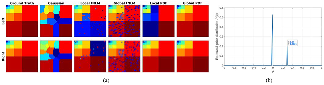
(a) Parcellation result of simulated data represented as a V × V matrix for each method and each hemisphere. The columns represent different filtering methods indicated by their titles along upper row. The rows represent the two hemispheres; (b) The estimated prior distribution of the population correlation under perfect within-block correlation setting (c = 1 and ρ = 0.284 in Equation (4)).
To investigate the effects of different filtering methods, we applied filtering to the simulated data then parcellated the data into K labels using the Normalized Cuts (NCuts) algorithm (Shi and Malik, 2000). A stable matching algorithm (Gale and Shapley, 2013) was applied to match labels between different results for easy comparison. Figure 2 (a) shows the parcellation results for: Gaussian filtering with full-width-half-maximum (FWHM) approximately 8 points (column 2); tNLM filtering with optimized h parameter (Li and Leahy, 2017) (column 3 and 4); local and global PDF filtering (column 5 and 6). To demonstrate the difference between local filtering and global filtering, we applied the tNLM filtering and PDF filtering both locally (column 3 and 5) and globally (column 4 and 6). Local filtering processed left and right hemispheres separately while global filtering processed them jointly.
Gaussian spatial filtering generated labels along the boundaries between true labels not seen in the ground truth. This is most likely due to blurring of uncorrelated but neighboring vertices. In contrast, tNLM and both local and global PDF filtering methods preserved the blocky structures. However, both PDF methods yielded much cleaner results than tNLM because tNLM has a larger contribution from the uncorrelated vertices at each filtered point as discussed above. Note that for both PDF methods and tNLM the parameter h had been optimized, in the latter case using Li and Leahy (2017), to achieve the best trade-off. Finally, for both tNLM and PDF, local filtering resulted in labels that were mismatched between the left and right hemispheres. The myopic perspective of local filtering failed to detect the distal, especially inter-hemispheric, connections. In contrast, GPDF was able to correctly identify inter-hemispheric connections and label appropriately.
Quantitatively, we ran this simulation for 100 Monte Carlo trials and calculated the Adjusted Rand Index (ARI) (Rand, 1971) between each parcellation result and the ground truth as a filtering performance measure. The medians of the ARIs were 0.547, 0.701, 0.760, 0.750, and 0.969 respectively in correspondence to each filtering method in Fig. 2 (a) column 2 – 6, indicating that GPDF outperformed other filtering methods by a significant margin.
Furthermore, GPDF not only produced the best clustering results among all filtering methods, but also correctly estimated the population correlation from the data. Figure 2 (b) shows the estimated distribution of the prior population correlation using Equation (11) under this perfect within-block correlation setting. The results show that the estimated prior , that contains the union of PH0(ρ) and PH1(ρ) as described above, has a bimodel distribution with two peaks, one at zero (corresponding to the zero between-block correlations) and another at 0.29 (corresponding to the non-zero within-block correlations), which matches very well with the simulated priors (c = 1 and ρ = 0.284 under H1 in Equation (4)).
Similar phenomena can be observed when nodes are partially correlated (c < 1 in Equation (4)) within each block without the presence of additional noise. The results for partial correlation c = 0.25, 0.5 and 0.75 with the same T = 200 and SNR = 0.4 are shown in the supplementary materials.
To investigate the robustness of GPDF over a variety of simulated settings, we evaluated the ARI between the parcellation result of filtered data (Gaussian, global tNLM and GPDF) and the ground truth as a function of the time-series length T as well as SNR. For each simulated dataset, we ran 100 Monte Carlo trials and boxplots were generated for each filtering method. Figure 3 shows the result of ARI as a function of T in (a) and SNR in (b).
Figure 3:
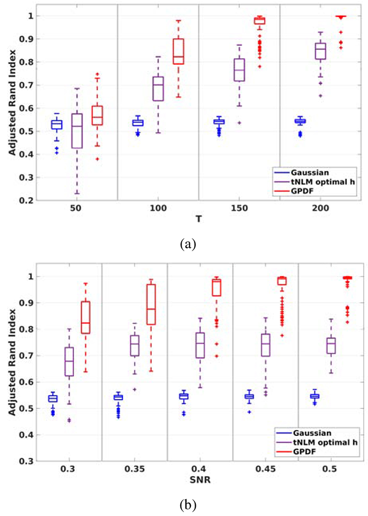
Robustness comparison of results using Gaussian filter, global tNLM filter with optimized parameter and GPDF. (a) ARI between parcellation result of filtered data and the ground truth as a function of time series length T with fixed SNR = 0.3; ARI between parcellation result of filtered data and the ground truth as a function of SNR with fixed T = 100
The performance of Gaussian filtering does not improve when T increases as the Gaussian filter applies a pure spatial kernel to data without using the temporal information between time series. In contrast, both the tNLM and GPDF filter show improved performance as T increases, but GPDF outperforms tNLM over the entire range of T.
When SNR varies with fixed T = 100, the ARI for the Gaussian filtered case increases but the performance is limited by the inevitable blurring effects across boundaries of different functional areas. Whereas, similar to (a), both tNLM and GPDF yield better parcellation results as SNR increases and higher ARI is obtained using GPDF-filtered data compared to tNLM.
3.2. Application to In-vivo Resting fMRI Dataset
3.2.1. Dataset and Filtering
40 subjects with minimally preprocessed rfMRI datasets (2 sessions, 2 phase encodings; 160 sessions total) were obtained from HCP (Van Essen et al., 2013). The data were acquired with TR = 720 ms with resolution 2 × 2 × 2 mm and had been preprocessed using the pipeline described in Glasser et al. (2013), where only minimal (2 mm FWHM) Gaussian smoothing was applied. Then the data were co-registered onto a common atlas and downsampled onto a 32K-vertex cortical surface. We further downsampled each data to 11K vertices for computational tractability.
We then filtered each dataset using Laplace-Beltrami (LB) smoothing with a range of values of smoothing parameter σ (the SD of the Gaussian kernel), tNLM with a range of values of the parameter h defined in Equation (3) and GPDF with a range of values of the parameter α defined in Equation (10). The effective δ in Equation (5) was chosen to be approximately 0.02 as described in Section 2.2.1. We performed three experiments: (i) exploration of correlation, community structure and modularity; (ii) seeded correlation; and (iii) comparison with task fMRI. In each case we compared GPDF with LB and tNLM both qualitatively and quantitatively. In the first experiment, we demonstrate the effect of filtering parameters (σ ∈ {1, 2, 3, 4, 5} mm, h ∈ {0.2, 0.4, 0.6, 0.8, 1} and α ∈ {10−1, 10−2, 10−3, 10−4, 10−5} in Section 3.2.2. For the other two experiments, we chose h = 0.4 for the tNLM method and α = 10−4 for the GPDF method, the optimal parameters from the first experiment. We chose σ = 3 mm for the LB method to avoid poor performance resulting from either under or over smoothing.
3.2.2. Unfiltered Correlation Matrix, Community Structure and Modularity
Modularity is a measure of community structure that can be used to identify sub-networks from brain connectivity data (Sporns and Betzel, 2016). Community structure can be directly visualized using the re-ordered connectivity matrix (equivalently, the correlation or association matrix) based on module detection or parcellation results. (See for example Fig. 2 (i) in Sporns and Betzel (2016)).
We use the same concept here to demonstrate the effect of filtering. For each dataset we took the unfiltered data and computed the full Pearson correlation matrix, , as the underlying graph structure. We then applied the NCuts algorithm (Shi and Malik, 2000) to parcellate the brain into K networks using each of the following: the unfiltered data, the LB-filtered data, the tNLM-filtered data and the GPDF-filtered data, generating parcellation labels for each of the four. We then used those labels to re-order the original connectivity matrix A so that vertices that have the same label are grouped together.
Figure 4 (a) – (d) show the re-ordered unfiltered connectivity matrix A based on the parcellation result (K = 7) using the unfiltered data, the LB-filtered data, the tNLM-filtered data and the GPDF-filtered data, respectively. Using the same (reordered) unfiltered connectivity matrix A establishes an unbiased comparison of the four partitions. The resulting re-ordered connectivity matrix indicates how well each filtering method grouped the data into functionally homogeneous regions with respect to the original (unfiltered) data. In essence, we assume that a better filtering method will give us a better clustering of nodes under a given parcellation algorithm: nodes with the same label (within the same network) tend to have higher as well as consistent correlations with each other than with nodes in other networks (diagonal blocks) and tend to have consistent correlation (can be either positive, zero or negative) with nodes in other networks (off-diagonal blocks). The GPDF result in Fig. 4 (d) shows a neat grouping of nodes forming a clearer blocky community structure and higher correlation in the diagonal blocks than all other cases shown in (a) - (c).
Figure 4:
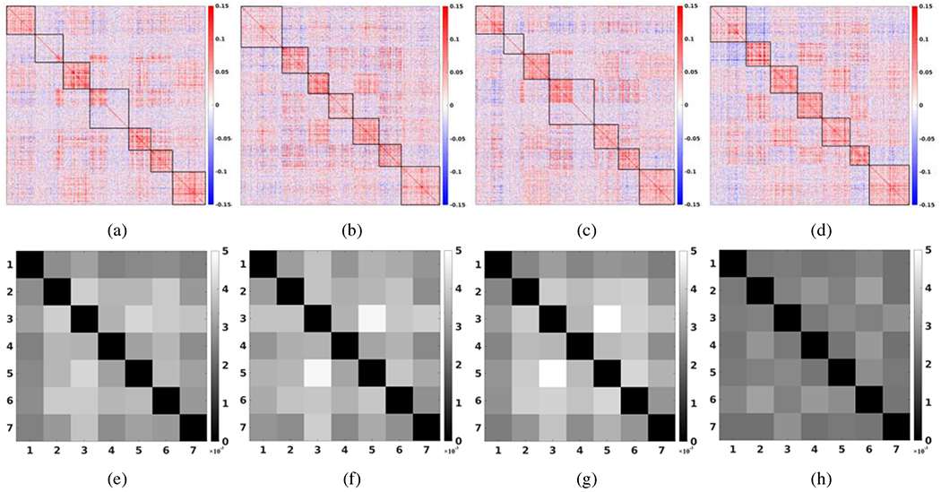
Re-ordered unfiltered full correlation matrices based on the parcellation result using (a) the unfiltered data, (b) LB-filtered data, (c) tNLM-filtered data and (d) GPDF-filtered data for K = 7. (e) - (h) shows the corresponding block-wise median SD map over 160 sessions for (a) - (d).
To quantitatively verify this observation, for each of the off-diagonal blocks in each fMRI recording session, we computed the SD of the correlation values within that block, yielding a K × K compressed SD map. Then we calculated the median SD over the 160 fMRI sessions. Figure 4 (e) – (h) show the median SD map for the unfiltered, the LB-filtered, the tNLM-filtered and the GPDF-filtered case, respectively, for K = 7. The GPDF result shows substantial lower SD in the off-diagonal blocks, indicating higher consistency among the nodes in one network with respect to the relationship to other networks. We observed similar phenomena for other values of K.
To further evaluate filtering performance and its robustness for a range of number of parcels K, for each unfiltered correlation matrix A, we binarized it with a threshold T to form a binary adjacency matrix A′. We then calculated the modularity (Newman, 2006) for A′ using each of the four K-network partitions (unfiltered, LB, tNLM, GPDF) as a function of T. The analyses were performed on each dataset independently. Figure 5 (a) shows the median modularity with standard error across 160 sessions as a function of T. The GPDF filtering method outperformed LB, tNLM and the unfiltered case regardless of the threshold T and the number of parcels, indicating that GPDF is producing parcellations with stronger within network similarity with respect to the unfiltered data than either the unfiltered case or tNLM or LB filtering.
Figure 5:
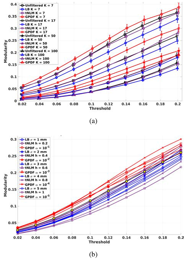
Network modularity plots. (a) The modularity as a function of the threshold T for different K and filtering methods with fixed filtering parameter σ = 3 mm, h = 0.4, and α = 10−4. The vertical bars represent the standard errors. The data points have been jittered slightly along the x-axis for a better visualization; (b) The modularity as a function of the threshold T for different filtering method and parameters with fixed K = 17.
Additionally, we investigated how the filtering parameters σ for LB, h for tNLM and α for GPDF influenced the filtering result. We computed the modularity as described above while varying σ ∈ {1, 2, 3, 4, 5} mm, h ∈ {0.2, 0.4, 0.6, 0.8, 1} and α ∈ {10−1, 10−2, 10−3, 10−4, 10−5} with fixed number of parcels K = 17. This number was selected for parcellation stability as suggested in Yeo et al. (2011). Figure 5 (b) shows the modularity as a function of T for each filtering parameter. Similar standard errors were observed as Fig. 5 (a) but were omitted here for clarity of the plot. For LB filtering, smaller σ yields similar results to the unfiltered case. Performance deteriorates as σ increases due to the increasing amount of blurring and mixing of signals across different functional regions. In general, LB filtering actually performs worse than the unfiltered case, regardless of the filtering parameter, when performing individual parcellations, suggesting that LB may not optimally preserve differences between individuals based on a single fMRI recording. For the tNLM method, slightly higher modularity than the unfiltered case was achieved for an optimal value of parameter h but performance then degrades significantly as h increases. In contrast, GPDF outperforms the unfiltered case, LB and tNLM, for most parameter settings except for large α with high T. This is because larger α allows a significant fraction of uncorrelated nodes to be involved in the filtered signal, resulting in worse performance as discussed in the introduction. We found α = 10−4 gives the best result in this experiment, which is the basis of our recommendation for a conservative α in the GPDF filtering method as described in Section 2.2.2.
3.2.3. Seeded Correlation Maps
Seed-based methods have been widely used in fMRI data analysis and brain network inference (Biswal et al., 1995; Di Martino et al., 2008; Taylor et al., 2009; Uddin et al., 2009). To evaluate the effects of filtering, we placed a seed point in the caudal pre-cuneus which is part of the Default Mode Network (DMN) (Fig. 6 (a)) and calculated the Pearson correlation of its time series with those of all other vertices of the brain, to form a correlation map.
Figure 6:
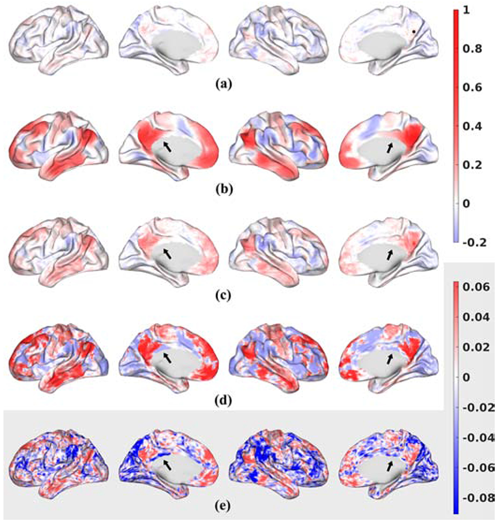
Seeded correlation map for a single subject for (a) Unfiltered data; (b) LB-filtered (σ = 3 mm) data; (c) tNLM-filtered (h = 0.4) data; (d) GPDF-filtered (α = 10−4) data plotted in a common scale from −0.2 to 1 with the color bar shown on the top right. (e) Unfiltered data re-plotted in its own narrow scale with color bar shown on the bottom right. Seed point was selected in the caudal pre-cuneus area shown as a black dot in (a). Positively correlated regions are shown in red, uncorrelated regions in white and negatively correlated regions in blue.
Figure 6 shows seed-point correlation maps for a single subject for the (a) unfiltered data; (b) LB-filtered data; (c) tNLM-filtered data and (d) GPDF-filtered data in a common scale ranging from −0.2 to 1. DMN can be seen in the unfiltered correlation map (a) but in the very low correlation range due to the rfMRI’s inherent low SNR. Figure 6 (e) exaggerates the color scale of unfiltered data for easy visualization of the correlation structure. LB, tNLM and GPDF, in contrast, yield higher correlations due to their ability to reduce noise and amplify signal. However, GPDF exhibits a wider range of correlation values than LB and tNLM.
Additionally, GPDF appears better able to preserves spatial delineation of adjacent regions with opposite correlation polarity relative to the seed point, for example two adjacent regions are indicated by the arrows in Fig. 6. Boundaries are clearly visible in both the unfiltered data (exaggerated in (e)) and GPDF, barely visible in tNLM but not in LB. These observations are indicative of LB’s tendency to spatially blur the boundaries between distinct adjacent functional areas.
LB shows strong connections to the local points surrounding the seed point while connections to distal areas, especially inter-hemispherical connections, are attenuated due to the localness of the filtering. This attenuation does not occur in GPDF as strong correlations are preserved across distal and inter-hemispheric regions of the DMN. GPDF therefore appears to help reveal stronger intra-network connectivity than the LB filtering method.
We also selected points that are highly correlated with the seed point and explored how those correlations were altered by filtering. A point was defined as being highly correlated with the seed point if its value in Fig. 6 (a) lay in either of the two tails of the null distribution H0 : P(r|ρ = 0, T = 1200) (overlaid in Fig. 7 (b), (c) and (d) with 10−6 significance level (the corresponding cut-off is 0.133)).
Figure 7:
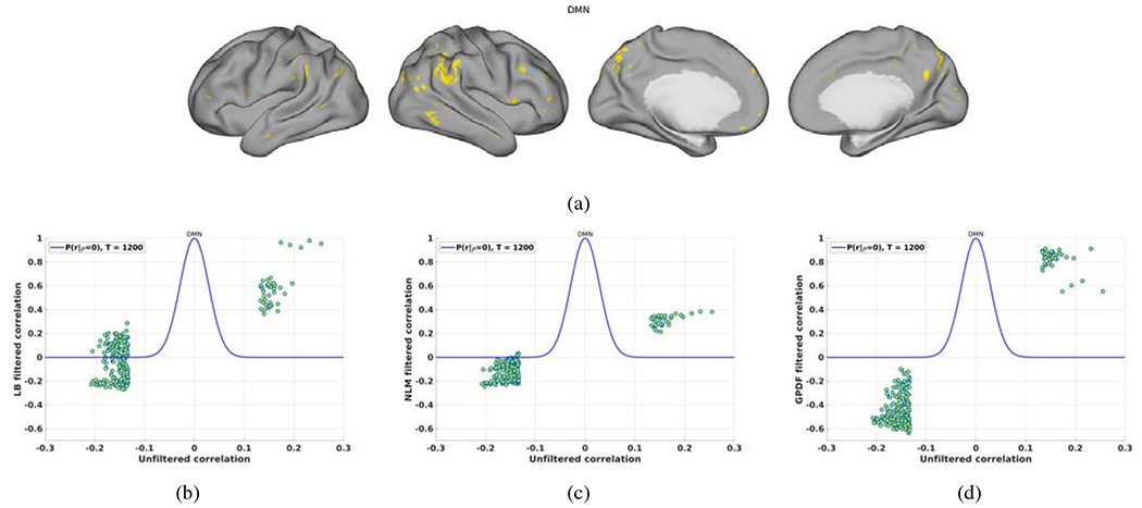
Changes of the seeded correlation values after filtering. (a) Spatial map of the highly correlated vertices to the seed point in the unfiltered data; (b) Scatter plot of the unfiltered correlation values of those vertices in (a) versus the LB-filtered correlation values overlaid with the null distribution P(r|ρ = 0) for T = 1200; (c) Similar to (b) but for the tNLM-filtered case; (d) Similar to (b) but for the GPDF-filtered case.
Figure 7 (a) shows the spatial locations in yellow of those points highly correlated with the seed. Figure 7 (b), (c) and (d) show the scatter plot between the unfiltered correlation (values of those points in Fig. 6 (a)) and the filtered correlation (values of those points in Fig. 6 (b), (c) and (d)) for LB, tNLM and GPDF, respectively. Both tNLM and GPDF amplify the positive correlation values but retain the sign of the correlation, Fig. 7 (c) and (d). This is expected since the non-local means kernel was designed to average only similar signals. The amplification effect is larger in the GPDF case due to the design of the shape of the kernel function. On the other hand, while LB also amplifies the correlation values, after filtering the signs of a substantial fraction of these correlation values have been flipped from negative to positive, Fig. 7 (b). This is caused by the blurring of signals across functional boundaries, indicating a potential confound when interpreting results from LB-filtered individual fMRI signals.
Similar results for other well known but less prominent networks, such as the motor network, the auditory network, the executive control network, the salience network, the frontoparietal attentional control network and the language network, are shown in the supplementary materials. Note that the seeded correlation maps may not show the desired networks exclusively due to overlap with other networks.
3.2.4. Parcellation Agreement with Task fMRI Activation Maps
Parcellation of rfMRI data is used to elucidate underlying spatial patterns in brain connectivity. However, the lack of an available ground truth makes it difficult to interpret parcellation results, especially when comparing different filtering methods. We tried to address this difficulty by comparing rfMRI parcellation results obtained from different filtering methods to the localized task-based fMRI (tfMRI) results for each individual rfMRI session.
Task fMRI datasets were also available and obtained from HCP for the same 40 subjects and they contained 7 major task domains: motor strip mapping (Motor), language processing (Language), emotion processing (Emotion), reward & decision-making (Gambling), relational processing (Relational), social cognition (Social) and working memory (WM). We used the preprocessed (4 mm Gaussian smoothed) and analyzed tfMRI z-score statistical maps from HCP, including a total of 15 task-pair as described in detail in Barch et al. (2013): tongue vs average (t_avg), left hand vs average (lh_avg), right hand vs average (rh_avg), left foot vs average (lf_avg) and right foot vs average (rf_avg) from the Motor task; math vs story (math_story) from the Language task; faces vs shapes (faces_shapes) from the Emotion task; punish vs reward (punish_reward) from the Gambling task; object matching vs geometrical relationship (match_rel) from the Relational task; random movement vs intentional movement (random_tom) from the Social task; 0-back vs 2-back (0bk_2bk), face vs average (face_avg), place vs average (place_avg), tool vs average (tool_avg), body vs average (body_avg) from the WM task.
To evaluate the performance of different filtering methods, for each individual fMRI session, we first parcellated the brain (rfMRI data) into K parcels using a spatially constrained hierarchical parcellation approach (Blumensath et al., 2013) for each of the filtering methods (unfiltered, LB, tNLM and GPDF). This “region growing”-based parcellation method is particularly appropriate for this tfMRI comparison purpose as it was designed to robustly parcellate the entire human cerebral cortex on a single subject basis. It also enforces spatial contiguity of the parcels, which allows us to obtain a reasonable parcellation result from unfiltered data (see Blumensath et al. (2013) for details).
Qualitatively, Fig. 8 shows the maps of the parcel boundaries for K = 100 parcels overlaid on the z-score maps of the Motor task t_avg contrast in (a) - (d) and Emotional task faces_shapes contrast in (e) - (h) for a single session of subject 100307. Figure 8 illustrates improved consistency of the parcellation boundaries with different functional regions (e.g., the tongue area and the fusiform face area) using GPDF filtering relative to the unfiltered case. In contrast, in the LB-filtered case, either some boundaries cross task-active areas or some parcels contain both task-positive and task-negative regions.
Figure 8:
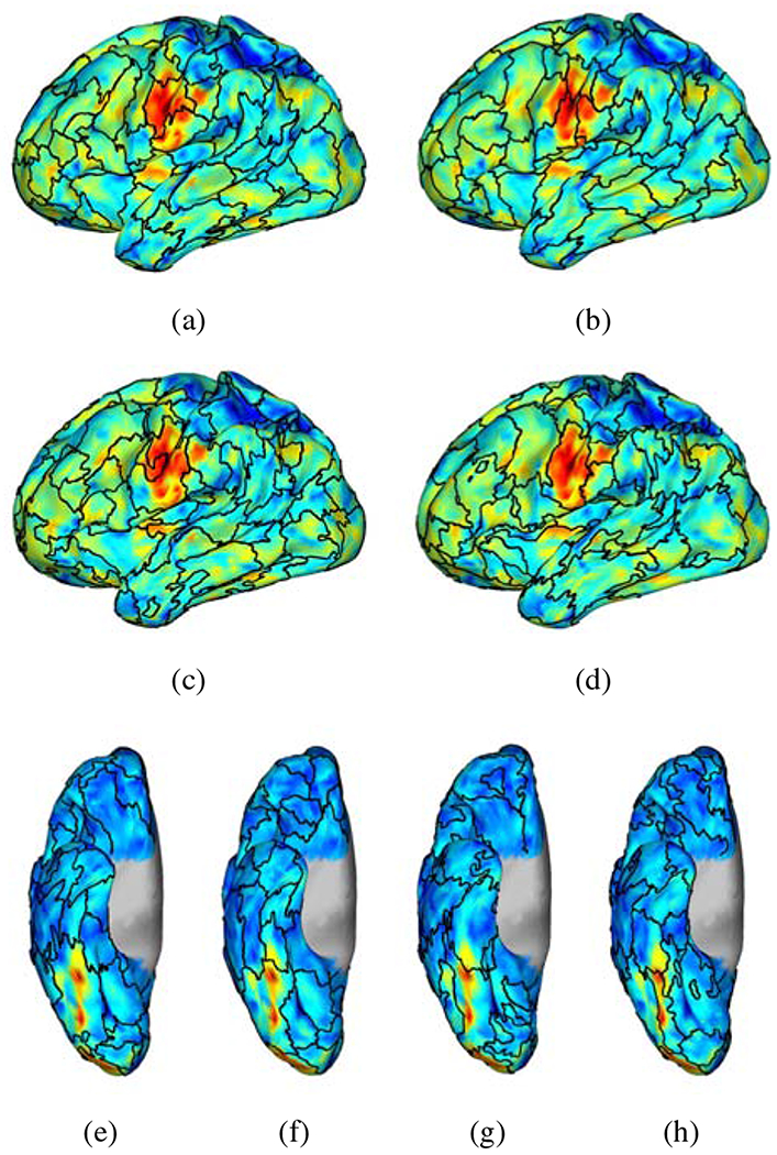
Maps of parcel boundaries overlaid with motor task tongue vs average contrast (a) - (d) and emotional task faces vs shapes (e) - (h) for a single session of subject 100307 using the unfiltered data ((a) and (e)), the LB-filtered (σ = 3 mm) data ((b) and (f)), the tNLM-filtered (h = 0.4) data ((c) and (g)) and the GPDF-filtered (α = 10−4) data ((d) and (h)). (Number of parcels K = 100)
To quantitatively measure performance for a certain task pair we first converted the z score map into a p-value map and thresholded the p-value map using Benjamini-Hochberg false discovery rate (Benjamini and Hochberg, 1995) correction with a q value of 0.05 to determine the activated vertices. Then in each parcel we counted the number of activated vertices and the counts from all parcels were sorted in a descending order and normalized to have unit sum, forming a positively skewed distribution. The larger the skewness, the higher concentration of the activated vertices into fewer parcels, hence the better alignment of the functional boundaries to the task-positive regions. We measured this skewness metric for all 15 task contrasts and all 160 individual fMRI sessions with different number of parcels K. Since there is no ground truth of the correct K that should be used for the parcellation, we selected K = K′ as the value that yielded the largest skewness in the unfiltered case for each task and each session independently (K′ varies substantially across different tasks and different sessions) and compared the skewness using the same K′ in all four cases (unfiltered, LB, tNLM and GPDF).
Figure 9 shows boxplots of skewness across 160 fMRI sessions for each task pair. The skewness of GPDF are consistently higher than the unfiltered, the LB-filtered as well as the tNLM-filtered case for all 15 task pairs, despite the fact that they vary from task to task.
Figure 9:
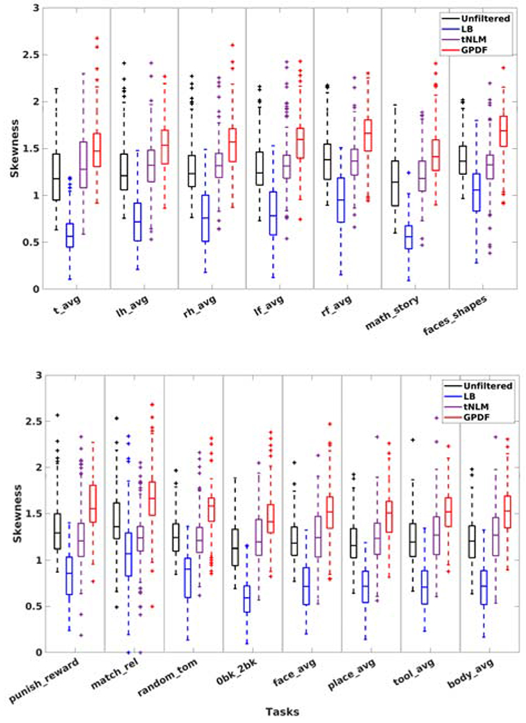
Boxplots of the skewness over 160 fMRI sessions for all 15 task pairs. Each column shows the boxplot for one particular task using the unfiltered data (far left), the LB-filtered data (middle left), the tNLM-filtered data (middle right) and the GPDF-filtered data (far right).
We also applied a Wilcoxon signed-rank test to determine if there was a significant improvement in skewness by filtering. The statistical results confirmed our visual observation and showed that GPDF filtering yields significantly higher skewness when compared with the unfiltered, the LB-filtered, and the tNLM-filtered case in all 15 task pairs. The median p-value across all 15 task pairs is 8.90 × 10⁻¹⁵, 2.69 × 10⁻²⁸ and 1.12 × 10⁻¹³ for the three comparison, respectively. The details of the test statistics and the associated p-values are given in the supplementary materials.
3.2.5. Computational Tractability
The time computational complexity is O(V2T), where V is the number of vertices/voxels and T is the number of time points. At the first stage of the GPDF algorithm when the kernel function and parameter is estimated, the entire correlation matrix is required to compute the histogram. The high computational burden can be significantly reduced by downsampling the data to a lower spatial resolution. Based on our experiments, the estimated kernel function and the parameter using the 11K data is almost identical to that using full resolution data.
At the second stage when we filter the data, however, no downsampling is needed and the computation can be performed in a vertex-wise manner at the whole brain level. We have implemented a block-wise filtering procedure where the vertices were divided into blocks and the filtering was performed iteratively over all blocks. The number of blocks was dynamically determined based on the memory available in the computer. This block-wise filtering achieves an effective trade-off between available memory and computation time. This implementation has been released for research purposes (see https://silencer1127.github.io/software/GPDF/gpdf_main). Based on our experiments, filtering a full resolution 96K HCP resting fMRI dataset (32K for left hemisphere + 32K right hemisphere + 32K sub-cortical voxels) takes approximately 7 minutes on a Dell desktop computer with an Intel Xeon E5-1650 v2 @ 3.50 GHz CPU and 16 GB RAM.
Since the filtering can be performance in vertex-wise manner, one may benefit from a customized GPU implementation to further accelerate the filtering procedure.
4. Discussion
In this paper, we systematically developed a novel kernel function based on the Bayes factor for global tNLM filtering. We also provided a way to automatically tune the parameter in order to achieve an optimal filtering result. We demonstrated both qualitatively and quantitatively using simulations as well as three experiments on in-vivo fMRI data that this method can simultaneously perform denoising that better preserves boundaries between regions of different functional specializations than standard linear filtering method.
The superior performance of GPDF filtering over the traditional linear filtering comes from the non-linearity of the kernel function visible as the black curve in Fig. 1. This effect can perhaps be most clearly seen in Fig. 8, where we evaluate how well task-activated regions are confined to parcels identified from individual resting data, with and without filtering. We note that linear (LB) filtering shows poorer performance than with unfiltered data. We believe this is because linear filtering inevitably produces blurring which can lead to misplacement of functional boundaries, or even generation of spurious functional regions along boundaries, as illustrated in Fig. 2. We show results in Fig. 8 for only one value of the LB smoothing parameter (σ = 3 mm). Performance could be improved by reducing σ, but with the limiting case of no filtering (σ = 0 mm) producing the best performance. We also note that the surface-based LB filtering used in our comparison is generally preferred over volumetric Gaussian filtering (Jo et al., 2007; Coalson et al., 2018) as volumetric filtering has partial volume effects in addition to the problem of spatial mixing of signals across different functional regions as discussed above. The performance of tNLM is variable in Fig. 8, outperforming the case for unfiltered data in some cases but not all. In contrast GPDF consistently shows significantly better performance compared to all methods. Note that the design of the kernel uses a data-driven approach, which can be different for different datasets. Therefore, it may be particularly useful when inferring brain connectivity patterns from individual fMRI recordings instead of a group analysis.
In some limiting cases, the kernel function may have a very sharp transition from zero weight to unit weight, forming a nearly binary kernel function, where vertices whose correlation exceed the threshold will be averaged together. However, even in this case it can be viewed as a valid filtering method rather than a parcellation method since each vertex has a distinct correlation pattern to all other vertices of the brain, thus the set of vertices over which the time series are averaged together can vary from vertex to vertex. Based on our experience, in most cases the kernel function exhibits a smoother non-linear transition rather than a binary thresholding.
One limitation of our approach is that the parametric model in Equation (6) for the distribution of the sample correlation assumes samples are independent over time. In practice, resting fMRI exhibit strong correlations which can result in higher variance than that predicted with this model (James et al., 2019; Afyouni et al., 2019). This will result in higher weights being applied to nodes with low correlation than would be the case if time samples were independent. A more conservative (smaller) choice of the α parameter can be used to offset this effect using the method as described here. An alternative approach that we have not pursued, is to explore alternatives to Equation (6) that account for correlation in the samples.
Another limitation is that the kernel function is estimated based on the empirical correlation using the entire time-series, which implicitly assume the stationarity of the fMRI signals. Extensions of this method to performing temporally dynamic filtering is a promising future direction.
Supplementary Material
Highlights.
Temporal non-local means filtering improves SNR but preserves functional boundaries
GPDF filtering with optimized kernel and parameter is crucial for optimal results
Individual parcellation results are substantially improved after GPDF filtering
Acknowledgments
Funding: This work was supported by the National Institutes of Health [grant number R01-NS089212, R01-NS074980, R01-EB026299].
Footnotes
Publisher's Disclaimer: This is a PDF file of an unedited manuscript that has been accepted for publication. As a service to our customers we are providing this early version of the manuscript. The manuscript will undergo copyediting, typesetting, and review of the resulting proof before it is published in its final form. Please note that during the production process errors may be discovered which could affect the content, and all legal disclaimers that apply to the journal pertain.
Declaration of interests
The authors declare that they have no known competing financial interests or personal relationships that could have appeared to influence the work reported in this paper.
References
- Afyouni S, Smith SM, Nichols TE, 2019. Effective degrees of freedom of the Pearson’s correlation coefficient under autocorrelation. NeuroImage 199, 609–625. doi: 10.1016/j.neuroimage.2019.05.011. [DOI] [PMC free article] [PubMed] [Google Scholar]
- Angenent S, 1999. On the Laplace-Beltrami operator and brain surface flattening. IEEE Transactions on Medical Imaging 18, 700–711. doi: 10.1109/42.796283. [DOI] [PubMed] [Google Scholar]
- Barch DM, Burgess GC, Harms MP, Petersen SE, Schlaggar BL, Corbetta M, Glasser MF, Curtiss S, Dixit S, Feldt C, Nolan D, Bryant E, Hartley T, Footer O, Bjork JM, Poldrack R, Smith S, Johansen-Berg H, Snyder AZ, Van Essen DC, 2013. Function in the human connectome: Task-fMRI and individual differences in behavior. NeuroImage 80, 169–189. doi: 10.1016/j.neuroimage.2013.05.033. [DOI] [PMC free article] [PubMed] [Google Scholar]
- Benjamini Y, Hochberg Y, 1995. Controlling the false discovery rate: a practical and powerful approach to multiple testing. Journal of the Royal statistical society: series B (Methodological) 57, 289–300. doi: 10.1111/j.2517-6161.1995.tb02031.x. [DOI] [Google Scholar]
- Bernier M, Chamberland M, Houde JC, Descoteaux M, Whittingstall K, 2014. Using fMRI non-local means denoising to uncover activation in sub-cortical structures at 1.5 T for guided HARDI tractography. Frontiers in Human Neuroscience 8, 715. doi: 10.3389/fnhum.2014.00715. [DOI] [PMC free article] [PubMed] [Google Scholar]
- Bhushan C, Chong M, Choi S, Joshi AA, Haldar JP, Damasio H, Leahy RM, 2016. Temporal non-local means filtering reveals real-time whole-brain cortical interactions in resting fMRI. PLoS ONE 11, 1–22. doi: 10.1371/journal.pone.0158504. [DOI] [PMC free article] [PubMed] [Google Scholar]
- Biswal B, Zerrin Yetkin F, Haughton VM, Hyde JS, 1995. Functional connectivity in the motor cortex of resting human brain using echo-planar MRI. Magnetic Resonance in Medicine 34, 537–541. doi: 10.1002/mrm.1910340409. [DOI] [PubMed] [Google Scholar]
- Blumensath T, Jbabdi S, Glasser MF, Van Essen DC, Ugurbil K, Behrens TE, Smith SM, 2013. Spatially constrained hierarchical parcellation of the brain with resting-state fMRI. NeuroImage 76, 313–324. doi: 10.1016/j.neuroimage.2013.03.024. [DOI] [PMC free article] [PubMed] [Google Scholar]
- Bro R, De Jong S, 1997. A fast non-negativity-constrained least squares algorithm. Journal of Chemometrics 11, 393–401. doi:. [DOI] [Google Scholar]
- Buades A, Coll B, Morel JM, 2005. A non-local algorithm for image denoising, in: Proceedings of the IEEE Computer Society Conference on Computer Vision and Pattern Recognition, pp. 60–65. doi: 10.1109/CVPR.2005.38. [DOI] [Google Scholar]
- Bullmore E, Sporns O, 2009. Complex brain networks: Graph theoretical analysis of structural and functional systems. Nature Reviews Neuroscience 10, 186–198. doi: 10.1038/nrn2575. [DOI] [PubMed] [Google Scholar]
- Coalson TS, Van Essen DC, Glasser MF, 2018. The impact of traditional neuroimaging methods on the spatial localization of cortical areas. Proceedings of the National Academy of Sciences of the United States of America 115, E6356–E6365. doi: 10.1073/pnas.1801582115. [DOI] [PMC free article] [PubMed] [Google Scholar]
- Coupe P, Yger P, Prima S, Hellier P, Kervrann C, Barillot C, 2008. An optimized blockwise nonlocal means denoising filter for 3-D magnetic resonance images. IEEE Transactions on Medical Imaging 27, 425–441. doi: 10.1109/TMI.2007.906087. [DOI] [PMC free article] [PubMed] [Google Scholar]
- Di Martino A, Scheres A, Margulies DS, Kelly AMC, Uddin LQ, Shehzad Z, Biswal B, Walters JR, Castellanos FX, Milham MP, 2008. Functional connectivity of human striatum: A resting state fMRI study. Cerebral Cortex 18, 2735–2747. doi: 10.1093/cercor/bhn041. [DOI] [PubMed] [Google Scholar]
- Fisher RA, 1915. Frequency distribution of the values of the correlation coefficient in samples from an indefinitely large population. Biometrika 10, 507. doi: 10.2307/2331838. [DOI] [Google Scholar]
- Gale D, Shapley LS, 2013. College admissions and the stability of marriage. American Mathematical Monthly 120, 386–391. doi: 10.4169/amer.math.monthly.120.05.386. [DOI] [Google Scholar]
- Glasser MF, Sotiropoulos SN, Wilson JA, Coalson TS, Fischl B, Andersson JL, Xu J, Jbabdi S, Webster M, Polimeni JR, Van Essen DC, Jenkinson M, 2013. The minimal preprocessing pipelines for the Human Connectome Project. NeuroImage 80, 105–124. doi: 10.1016/j.neuroimage.2013.04.127. [DOI] [PMC free article] [PubMed] [Google Scholar]
- James O, Park H, Kim SG, 2019. Impact of sampling rate on statistical significance for single subject fMRI connectivity analysis. Human Brain Mapping 40, 3321–3337. doi: 10.1002/hbm.24600. [DOI] [PMC free article] [PubMed] [Google Scholar]
- Jo HJ, Lee JM, Kim JH, Shin YW, Kim IY, Kwon JS, Kim SI, 2007. Spatial accuracy of fMRI activation influenced by volume- and surface-based spatial smoothing techniques. NeuroImage 34, 550–564. doi: 10.1016/j.neuroimage.2006.09.047. [DOI] [PubMed] [Google Scholar]
- Kass RE, Raftery AE, 1995. Bayes factors. Journal of the American Statistical Association 90, 773–795. doi: 10.1080/01621459.1995.10476572. [DOI] [Google Scholar]
- Li J, Choi S, Joshi AA, Wisnowski JL, Leahy RM, 2018. Global PDF-based temporal non-local means filtering reveals individual differences in brain connectivity, in: IEEE 15th International Symposium on Biomedical Imaging, pp. 15–19. doi: 10.1109/ISBI.2018.8363513. [DOI] [PMC free article] [PubMed] [Google Scholar]
- Li J, Leahy RM, 2017. Parameter selection for optimized non-local means filtering of task fMRI, in: IEEE 14th International Symposium on Biomedical Imaging, Melbourne. pp. 476–480. doi: 10.1109/ISBI.2017.7950564. [DOI] [Google Scholar]
- Manjon JV, Carbonell-Caballero J, Lull JJ, Garcia-Marti G, Marti-Bonmati L, Robles M, 2008. MRI denoising using non-local means. Medical Image Analysis 12, 514–523. doi: 10.1016/j.media.2008.02.004. [DOI] [PubMed] [Google Scholar]
- Newman MEJ, 2006. Modularity and community structure in networks. Proceedings of the National Academy of Sciences 103, 8577–8582. doi: 10.1073/pnas.0601602103. [DOI] [PMC free article] [PubMed] [Google Scholar]
- Ogawa S, Lee TM, Kay AR, Tank DW, 1990. Brain magnetic resonance imaging with contrast dependent on blood oxygenation. Proceedings of the National Academy of Sciences of the United States of America 87, 9868–9872. doi: 10.1073/pnas.87.24.9868. [DOI] [PMC free article] [PubMed] [Google Scholar]
- Rand WM, 1971. Objective criteria for the evaluation of clustering methods. Journal of the American Statistical Association 66, 846–850. doi: 10.1080/01621459.1971.10482356. [DOI] [Google Scholar]
- Shi J, Malik J, 2000. Normalized cuts and image segmentation, in: IEEE Transactions on Pattern Analysis and Machine Intelligence, pp. 888–905. doi: 10.1109/34.868688. [DOI] [Google Scholar]
- Smith SM, Beckmann CF, Andersson J, Auerbach EJ, Bijsterbosch J, Douaud G, Duff E, Feinberg DA, Griffanti L, Harms MP, Kelly M, Laumann T, Miller KL, Moeller S, Petersen S, Power J, Salimi-Khorshidi G, Snyder AZ, Vu AT, Woolrich MW, Xu J, Yacoub E, Uurbil K, Van Essen DC, Glasser MF, 2013. Resting-state fMRI in the Human Connectome Project. NeuroImage 80, 144–168. doi: 10.1016/j.neuroimage.2013.05.039. [DOI] [PMC free article] [PubMed] [Google Scholar]
- Smith SM, Fox PT, Miller KL, Glahn DC, Fox PM, Mackay CE, Filippini N, Watkins KE, Toro R, Laird AR, Beckmann CF, 2009. Correspondence of the brain’s functional architecture during activation and rest. Proceedings of the National Academy of Sciences 106, 13040–13045. doi: 10.1073/pnas.0905267106. [DOI] [PMC free article] [PubMed] [Google Scholar]
- Sporns O, Betzel RF, 2016. Modular brain networks. Annual Review of Psychology 67, 613–640. doi: 10.1146/annurev-psych-122414-033634. [DOI] [PMC free article] [PubMed] [Google Scholar]
- Taylor KS, Seminowicz DA, Davis KD, 2009. Two systems of resting state connectivity between the insula and cingulate cortex. Human Brain Mapping 30, 2731–2745. doi: 10.1002/hbm.20705. [DOI] [PMC free article] [PubMed] [Google Scholar]
- Uddin LQ, Kelly AMC, Biswal BB, Castellanos FX, Milham MP, 2009. Functional connectivity of default mode network components: Correlation, anticorrelation, and causality. Human Brain Mapping 30, 625–637. doi: 10.1002/hbm.20531. [DOI] [PMC free article] [PubMed] [Google Scholar]
- Van Essen DC, Smith SM, Barch DM, Behrens TE, Yacoub E, Ugurbil K, 2013. The WU-Minn Human Connectome Project: An overview. NeuroImage 80, 62–79. doi: 10.1016/j.neuroimage.2013.05.041. [DOI] [PMC free article] [PubMed] [Google Scholar]
- Wiest-Daessle N, Prima S, Coupé P, Morrissey SP, Barillot C, 2008. Rician noise removal by non-local means filtering for low signal-to-noise ratio MRI: Applications to DT-MRI, in: International Conference on Medical Image Computing and Computer-assisted Intervention, Springer; pp. 171–179. doi: 10.1007/978-3-540-85990-1_21. [DOI] [PMC free article] [PubMed] [Google Scholar]
- Yeo BT, Krienen FM, Sepulcre J, Sabuncu MR, Lashkari D, Hollinshead M, Roffman JL, Smoller JW, Zollei L, Polimeni JR, Fischl B, Liu H, Buckner RL, 2011. The organization of the human cerebral cortex estimated by intrinsic functional connectivity. Journal of Neurophysiology 106, 1125–1165. doi: 10.1152/jn.00338.2011. [DOI] [PMC free article] [PubMed] [Google Scholar]
Associated Data
This section collects any data citations, data availability statements, or supplementary materials included in this article.