Multi‐ATOM: Ultrahigh‐throughput single‐cell quantitative phase imaging with subcellular resolution

Abstract

A growing body of evidence has substantiated the significance of quantitative phase imaging (QPI) in enabling cost‐effective and label‐free cellular assays, which provides useful insights into understanding the biophysical properties of cells and their roles in cellular functions. However, available QPI modalities are limited by the loss of imaging resolution at high throughput and thus run short of sufficient statistical power at the single‐cell precision to define cell identities in a large and heterogeneous population of cells—hindering their utility in mainstream biomedicine and biology. Here we present a new QPI modality, coined multiplexed asymmetric‐detection time‐stretch optical microscopy (multi‐ATOM) that captures and processes quantitative label‐free single‐cell images at ultrahigh throughput without compromising subcellular resolution. We show that multi‐ATOM, based upon ultrafast phase‐gradient encoding, outperforms state‐of‐the‐art QPI in permitting robust phase retrieval at a QPI throughput of >10 000 cell/sec, bypassing the need for interferometry which inevitably compromises QPI quality under ultrafast operation. We employ multi‐ATOM for large‐scale, label‐free, multivariate, cell‐type classification (e.g. breast cancer subtypes, and leukemic cells vs peripheral blood mononuclear cells) at high accuracy (>94%). Our results suggest that multi‐ATOM could empower new strategies in large‐scale biophysical single‐cell analysis with applications in biology and enriching disease diagnostics.

An ultrafast quantitative phase imaging (QPI) modality, called multiplexed asymmetric‐detection time‐stretch optical microscopy, is reported that enables ultra‐large‐scale, multicontrast, label‐free single‐cell imaging without compromising subcellular resolution. This capability, otherwise challenging in current QPI, critically enables high label‐free statistical discrimination power to allow multivariate cell‐type classification at high accuracy (>94%), suggesting its potential to empower new strategies in large‐scale biophysical single‐cell analysis with applications in biology and enriching disease diagnostics.

1. INTRODUCTION

Quantitative phase imaging (QPI) allows label‐free, noninvasive quantification of the local optical path length of biological specimens 1, 2, 3 that can be harnessed to gain insight into the cellular biophysical properties. This capability has advanced our understanding of cell biology and has enabled novel strategies in biomedical diagnostics. For example, cell size and mass evaluated from the quantitative phase are linked to cellular progression and apoptosis 4, 5. Subtle changes in subcellular organizations visualized in QPI can be used as a hallmark of cancer 6, 7, 8. When it comes to probing the biophysical properties at single‐cell precision, QPI could thus be of functional significance in complementing the current state‐of‐the‐art single‐cell analysis (SCA) 9, 10 in a cost‐effective manner.

Unfortunately, the widespread utility of QPI for biophysical phenotyping in SCA remains limited. The major challenge is that current QPI methodologies lack the ability to simultaneously deliver the two critical, but often conflicting attributes, that is, subcellular resolution and high imaging throughput, both of which are essential for assessing cell population heterogeneity with high discriminatory power. In the current QPI approaches, the subcellular resolution is commonly achieved at the expense of the imaging throughput which is limited to only a few tens to hundreds of cells within a field of view (FOV) 11. Despite that the throughput problem can partially be alleviated through automated sample scanning (up to ~10⁴ cells) 12, it is further exacerbated by the inherent limitations of current camera technology, that is, severe image motion blur, degradation in image resolution and loss of detection sensitivity at high speed. This also explains the limited flow rate and thus single‐cell imaging throughput in the available QPI flow cytometers 13, 14, 15. Even if they were integrated with the state‐of‐the‐art imaging flow cytometers, the imaging throughput is still ~1000 cells/s 16—significantly below the gold‐standard nonimaging flow cytometers ~100 000 cells/s.

By contrast, optical time‐stretch imaging offers a unique speed advantage over the conventional camera technologies, by achieving continuous frame rate of megahertz or beyond in real time for high‐throughput single‐cell imaging in flow (eg, 0.4 Gpixels/s in scientific Complementary Metal–Oxide–Semiconductor (sCMOS) vs 4 Gpixels/s in time‐stretch imaging) 17, 18, 19, 20, 21. Further empowered by interferometry, this technology enables ultrafast QPI for label‐free, cancer cell classification 22, 23. However, revealing subcellular features remains challenging in interferometric time‐stretch QPI. The major barrier is the exceedingly high group velocity dispersion (GVD) required for achieving diffraction‐limited imaging resolution that inevitably comes at the cost of severe optical loss and thus image signal‐to‐noise ratio (SNR) 24, 25. Consequently, the degraded SNR lowers the yield of phase‐image retrieval and hinders subcellular resolution in ultra‐large‐population single‐cell time‐stretch QPI (practically >10⁵ cells), which has yet been reported so far 23, 26.

Here, we present a new single‐cell QPI platform, coined multiplexed asymmetric‐detection time‐stretch optical microscopy (multi‐ATOM) that addresses these challenges and thus fills the gap for achieving large‐population single‐cell biophysical phenotyping at subcellular resolution. We demonstrate that multi‐ATOM can capture subcellular‐resolution single‐cell QPI images at an ultrahigh‐throughput in real time, at least two orders‐of‐magnitude faster than classical QPI. Multi‐ATOM also outperforms the existing time‐stretch QPI modalities in three critical aspects: (a) bypassing interferometry, multi‐ATOM features with ultrafast multiplexed phase‐gradient image encoding without excessive GVD and thus loss for achieving subcellular QPI resolution; (b) multi‐ATOM relies on intensity‐only phase‐retrieval algorithm critically guarantees high yield of quantitative phase reconstruction and thus robust single‐cell biophysical phenotyping; (c) thanks to its subcellular resolution preserved at high‐throughput, multi‐ATOM enables exploration of an additional image contrast, namely, dry‐mass‐density contrast (DC) map, that is sensitive to the local variation of dry mass density (DMD) within the cell and could allow subcellular biophysical SCA at large scale. As a proof‐of‐concept demonstration, we show that multi‐ATOM provides sufficient label‐free discrimination power for distinguishing two human breast cancer subtypes. It also allows ultra‐large‐scale label‐free image‐based classification of human leukemic cells and human peripheral blood monocular cells (PBMCs) (>700 000 cells) at high accuracy (>94%). We, therefore, anticipate multi‐ATOM could find its immediate potential utilities in label‐free cancer cell screening in blood.

2. RESULTS AND DISCUSSIONS

2.1. Working principles of multi‐ATOM

Multi‐ATOM leverages the concept of optical time‐stretch imaging, which implements all‐optical image encoding in and retrieval from the broadband laser pulses at an ultrafast line‐scan rate (equivalent to the laser repetition rate, i.e., 11.8 MHz in our case) (Figure 1A). It is achieved by two image mapping steps: wavelength‐time mapping (i.e., time‐stretch process) through GVD of light in a dispersive fiber and wavelength–space mapping (i.e., spectral‐encoding process) done by spatial dispersion of light using a diffraction grating 17, 20. Effectively, these two steps enable all‐optical laser line‐scanning imaging in which the image contrast at each imaged position is encoded with a different wavelength within the spectrum of the laser pulse. Here, the cells are in a unidirectional microfluidic flow orthogonal to the line scans, which can be digitally stacked to form a two‐dimensional (2D) image. In contrast to conventional time‐stretch QPI, the distinct feature of multi‐ATOM is its ability to encode the local phase gradients of the cells—a quantitative image contrast that has largely been overlooked in the existing time‐stretch imaging modalities and yet can be harnessed to obtain the quantitative phase of cells without interferometry.

Figure 1.

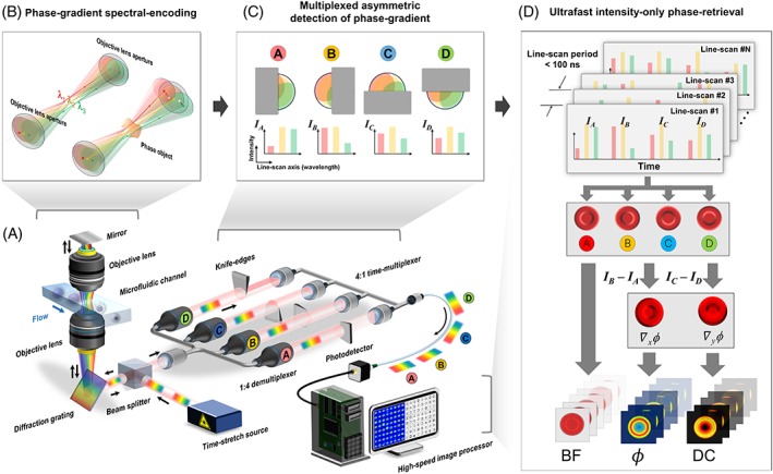
Working principle of multiplexed asymmetric‐detection time‐stretch optical microscopy. (A) System configuration: The ultrafast line‐scan pulsed beam is demultiplexed into four replicas (A‐D) after spectrally encoding the spatial phase gradient of the flowing cells (flow rate > 1 m/s). Each of these replicas is half‐blocked by a knife‐edge, followed by time‐multiplexing using the fiber delay lines and real‐time signal capture, digitization and processing. (B) Phase‐gradient spectral encoding: Each minimum spectrally resolvable beams of the line scan (ie, beam λ₁, λ₂ and λ₃, each representing different wavelength) is tilted according to the local phase gradient of phase object (ie, cell) and is thus partially collected by the objective lens. (C) Multiplexed asymmetric detection of phase gradient: Partial‐beam‐blocking of each beam replica (A‐D) from four cardinal directions results in four different transmitted intensity profiles along the spectrally encoded line scan, which are used to decode the magnitude and direction of the 2D local phase gradient. (D) Ultrafast intensity‐only phase retrieval: the image‐encoded line scans (each contains four time‐multiplexed replicas) is digitally stacked to form four 2D asymmetrically detected images (A‐D) and thus bright‐field and two phase‐gradient images (∇ϕ_x and ∇ϕ_y), from which quantitative‐phase (ϕ) images and dry‐mass‐density contrast maps are reconstructed

Under the condition that spectrally encoded line‐scan illumination is temporally incoherent, the phase gradient and thus quantitative phase across the cell can simply be modeled using geometrical optics (See Section 4 for details). This model rests on the fact that the local phase gradient of the phase object (i.e., cells) leads to wavefront tilt for each minimum spectrally resolvable spots of the line scan and thus partial‐light collection by the imaging objective lenses (Figure 1B and S1). Such light tilt from the image plane is equivalent to transverse displacement of the minimum spectrally resolvable beam in far‐field or on the Fourier plane. In essence, such displacement can be inferred by the fractional intensity loss of each resolvable beam. Hence, the magnitude variation in the phase gradient of the cells along the line scan, which is spectrally encoded in a single‐shot pulse, can be linked to the measured intensity profile across the spectrum.

To evaluate both the magnitude and direction of the 2D local phase gradient, multiple independent measurements of the intensity losses due to light tilt along the x‐ and y‐directions are required. It is easily done by splitting the encoded pulsed beam into four replicas and partially blocking them by the Foucault‐knife‐edge method from four cardinal directions before being coupled into four optical fibers (Figure 1C). The partial‐beam block effectively results in an asymmetric beam coupling into the four fibers, which capture the intensities, I _A(x,y), I _B(x,y), I _C(x,y), and I _D(x,y) that are linked to the phase gradient along the four cardinal directions. We previously adopted a similar beam‐block concept for enhancing the image contrast of label‐free time‐stretch imaging 19, 27. However, this method does not warrant the access to quantitative phase. It is because only the phase‐gradient contrast along one dimension is obtained whereas complete quantitative phase requires the information of the phase‐gradient contrasts along the two orthogonal dimensions. Quantifying the amplitude and direction of the phase‐gradient contrast for time‐stretch QPI has thus not been demonstrated until now. Here, multi‐ATOM goes beyond by exploiting multiple sets of spectrally encoded phase‐gradient contrasts along four cardinal directions to retrieve the quantitative phase. More precisely, the phase gradients along the x‐ and y‐directions (∇ϕ_x (x,y) and ∇ϕ_y (x,y)) are linked to the normalized intensity losses R _x(x, y) and R _y(x, y), which are proportional to the difference images, that is, I _B – I _A and I _C – I _D, respectively (Figures 1D and 2A, and see Section 4). The quantitative phase image, ϕ, (Figures 1D and 2A) from the phase gradients is evaluated by complex Fourier integration with a calibration factor obtained through imaging a known quantitative phase target. Note that only the intensities of the four images are needed and no iterative process is involved for phase retrieval. Other than the quantitative phase, the bright‐field contrast, that is, BF (Figure 1D) can also be obtained from the four asymmetrically detected signals (see Section 4). To ensure ultrafast operation, four replicas are captured by a time‐multiplexing scheme: replicas are firstly coupled into four individual fiber delay lines, each with different length, and then recombined by a multiplexer to become temporally separated. Eventually, these replicas are captured within each single‐shot line‐scan period (~84 ns) to achieve ultrafast QPI (Figures 1D and 2A).

Figure 2.

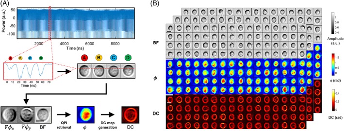
Image reconstruction pipeline illustration and representative cell images. (A) Image reconstruction: The continuous data stream is first truncated into data segments that each records a single cell. A single segment consists of a few tens of line scan, within each four pulse replicas are time‐multiplexed (zoom‐in windows). By reshaping the segment, an image including four asymmetric‐detection contrast subimages from the same single cell can be obtained (A‐D) from which two phase‐gradient‐constrast (∇ϕ_x and ∇ϕ_y) and a bright‐field contrast (BF) images are arithmetically combined. Based upon, a quantitative‐phase image (ϕ) is then retrieved by complex Fourier integration as well as the dry‐mass‐density contrast (DC) image. (B) Representative multicontrast multiplexed asymmetric‐detection time‐stretch optical microscopy cell images: BF, ϕ and DC single‐cell images of leukemic cells (THP‐1) which are captured at a throughput of >10 000 cell/sec. Scale bar = 10 μm

We can derive a multitude of image features, as the biophysical phenotypes of the cells, from both the quantitative phase and BF images. For instance, we extract the typical bulk parameters, for example, cell volume, roundness, optical opacity from the BF image whereas averaged dry mass and DMD from the phase image (see Table S1 for a detailed derivation). Beyond that, taking the advantage of the subcellular resolution preserved at high throughput in multi‐ATOM, we further transform each quantitative phase image into a DC map which visualizes and quantifies the local variation of DMD across the cell (Figure 2A and S2 and Table S1 ). We can thus extract additional subcellular resolvable phenotypes by quantifying the statistics of local DC of individual cells, such as DC1, DC2 and DC3 as the first‐, second‐ and third‐order statistical moments of DC which relate to the variation and the skewness of local DC distribution, respectively (Table S1 ). We note that the statistics of DC values across the cell are thus different from the global phase statistics obtained directly from the phase image 5. Altogether, multi‐ATOM enables label‐free single‐cell biophysical phenotypic profiling within an enormous population of cells, as discussed in the later section.

2.2. Imaging performance of multi‐ATOM

We evaluated the basic performance of multi‐ATOM in terms of its resolution, phase accuracy and stability. From the retrieved phase image of the phase target, the height profile of the USAF resolution chart target was measured to be ~100 nm, consistent to the target specification (Figure S3A,B). The corresponding QPI spatial resolution was also measured as 1.38 and 0.98 μm along the spectral encoding (fast axis) and sample scanning (slow‐axis) direction, respectively, according to the smallest features resolved by multi‐ATOM (ie, group 8 element 4 and group 9 element 1, respectively, in Figure S3A, B). On the other hand, the shot‐to‐shot fluctuations and the long‐term stability of the measured optical path lengths (derived from quantitative phase) over 4 hours were measured to be 4.5 nm (8.8 mrad) and 8.3 nm (16.2 mrad), respectively (Figure S3D). It demonstrates the high stability of multi‐ATOM, contributed by its interferometry‐free measurement, which is less sensitive to ambient mechanical perturbation. We next characterized the cell imaging performance of multi‐ATOM in a microfluidic flow at an imaging throughput of >10 000 cells/s (Figure 2A,B). Multi‐ATOM clearly shows the ability to capture motion‐blur‐free amplitude, phase‐gradient, phase and DC images of individual fast‐flowing cells (2.3 m/s) and reveal their subcellular textures at an ultrafast imaging rate (a line‐scan rate of 11.8 MHz)—a combined capability absents in both conventional camera‐based QPI and interferometric time‐stretch QPI (Figure 2B).

Achieving high spatial resolution in any time‐stretch imaging modalities is often complicated by the interplay among GVD, optical loss and data sampling rate 25. Notably, the exceedingly high sampling rate is required to reduce GVD and dispersive loss. But this condition can only be achieved in the high‐end oscilloscopes (typically >40 GSa/s) at the expense of high throughput continuous single‐cell image capture in real time. On the other hand, using the system with the lower sampling rate (e.g., field programmable gate array [FPGA] platform typically at <10 GSa/s) could improve the throughput performance at the cost of considerably higher GVD required for achieving diffraction‐limited resolution 28. The GVD requirement becomes even more stringent in interferometric time‐stretch QPI (or interferometric time‐stretch microscopy [iTM] 24), where extra GVD is required to ensure high fringe visibility of the spectrally encoded interferogram, and thus diffraction‐limited QPI. However, such an excessive GVD inevitably results in a significant optical loss, and thus degrades the imaging sensitivity.

In contrast, multi‐ATOM bypasses the use of interferometry. This offers the key advantages of mitigating the stringent demand for high GVD and preserving subcellular resolution at high imaging throughput. To demonstrate such significance, we configured an integrated system, which enables simultaneous multi‐ATOM and iTM of the identical cells under a diffraction‐limited resolution condition (Figures 3A and S4 and Section S1.2 in Appendix S1), and evaluated the effect of GVD on the performance in the two modalities (Figure 3 and Section 4 ). According to time‐stretch theory, changing GVD at a fixed sampling rate has the equivalent effect on image resolution to varying the sampling rate at a fixed GVD 29. Hence, here we study the GVD effect at the fixed sampling rate adopted in this work (4 GSa/s) by defining a range of equivalent GVD (GVD_eq), which is governed by the inverse relationship between GVD and sampling rate (see the detailed theory in Section 4).

Figure 3.

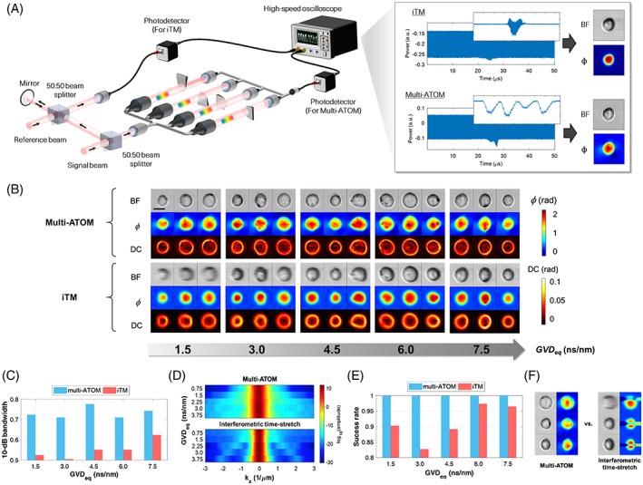
Performance comparison between multi‐ATOM and iTM. (A) System configuration: Each cell is simultaneously imaged by multi‐ATOM and iTM methods. (B) Image quality: The reconstructed images of each cell, with bright‐field, quantitative phase (ϕ) and dry‐mass‐density contrast image contrasts, are compared under five different GVD_eq conditions (Section 4). (C‐D) Spectral bandwidth analysis: (C) Averaged 10‐dB bandwidth of ϕ images (along the fast axis) and (D) the corresponding spectra obtained from both systems at different GVD_eq. Colorbar: logarithmic amplitude. (E and F) Phase‐retrieval yield analysis: (E) Comparison of the success rate of phase retrieval between multi‐ATOM and iTM based on captured images of approximately 4600 cells and (F) three representative failed cases of phase retrieval of iTM. GVD_eq, equivalent group velocity dispersion; iTM, interferometric time‐stretch microscopy; multi‐ATOM, multiplexed asymmetric‐detection time‐stretch optical microscopy

In general, except the overall cell shape is visualized, the subcellular texture is lost in iTM images as compared with that of multi‐ATOM (Figure 3B). Although the resolution of iTM increases with GVD _eq, which can be quantified in the corresponding signal bandwidth, the resolution in multi‐ATOM generally remains higher than that in iTM (Figure 3C, D). According to time‐stretch imaging resolution analysis 21, 25, 28, at least two times higher in GVD is required in iTM (2.29 ns/nm) compared to multi‐ATOM (1.14 ns/nm), in order to achieve similar imaging resolution (Figure S5 in Appendix S1). The resolution advantage of multi‐ATOM compared to iTM becomes more obvious when we further transform the quantitative phase image into a 2D DC map, which reveals more clearly the subcellular structures using multi‐ATOM (Figure 3B).

Another benefit from the interferometry‐free operation is that the quantitative phase retrieval in multi‐ATOM bypasses the need for the iterative phase unwrapping algorithms commonly used in QPI 30, 31, 32. Not only can it reduce the computational complexity which favors ultrafast real‐time image processing, but also, more importantly, eliminates the phase unwrapping error which is susceptible to noise and low fringe visibility 22, 29. Hence, phase retrieval in multi‐ATOM is essentially error‐free compared to that in iTM (Figure 3E,F). Note that the reduction in success rate in iTM (ie, ~5%‐15%) may not be tolerable in view of practical detection of small populations in an ultra‐large‐scale analysis of heterogeneous cell population, not to mention the even worse success rate in reality because of an extra 10‐dB degradation of SNR accompanied with doubling the GVD for achieving subcellular resolution.

2.3. Single‐cell image‐based biophysical phenotyping and classification using multi‐ATOM

We investigated the ability of multi‐ATOM‐derived single‐cell biophysical phenotypes, especially the subcellularly resolvable features, to discriminate two breast cancer lines, MCF‐7 and MDA‐MB‐231 33, which represents two subtypes of breast carcinoma (Figure 4A). Both the DC parameter (i.e., DC1) and opacity are found effective, as label‐free biophysical markers, to distinguish the two cell types in a mixed population (Figure 4B and see also the verification of the pure populations shown in Figure S6). In contrast, such mixture of two populations is not resolvable in standard flow cytometry based on scatter light measurements (inset of Figure 4B)—signifying the significance of quantitative label‐free, high‐resolution imaging for cytometry applications.

Figure 4.

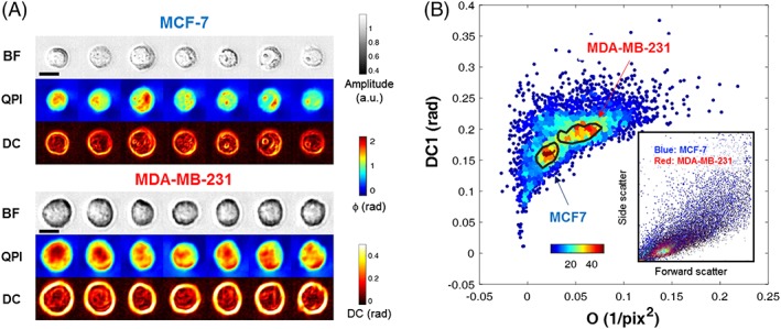
Label‐free classification of two breast cancer cell types. (A) Representative cell images: bright field, quantitative phase imaging and dry‐mass‐density contrast single‐cell images of two types of breast cancer cells (top: MCF‐7, bottom: MDA‐MB‐231). Scale bar = 10 μm. (B) Discrimination power of multi‐ATOM‐derived features: A bivariate density plot from multi‐ATOM showing distinctive distributions for two cancer cell types with the 60%‐density‐contours overlaid, while that of conventional flow cytometer (inset) shows an highly overlaped distribution. Color bar: local density of data points. multi‐ATOM, multiplexed asymmetric‐detection time‐stretch optical microscopy

We further assessed the high‐throughput capability of multi‐ATOM in ultra‐large‐scale single‐cell imaging (more than 700 000 cells). The underlying rationale is that the combined advantage of high‐throughput and high‐resolution imaging brought by multi‐ATOM could provide sufficient statistical power in single‐cell biophysical phenotyping, which was once regarded to lack the specificity for cell‐based assay, to reveal the diversity of cell populations. This is evident from the heterogeneity revealed in the bivariate plots (subcellular texture phenotype DC2 vs volume) of both cell types, especially the PBMC sample, which is known to be highly heterogeneous (Figure 5A,B). Precisely because of such diversity, a high‐dimensional biophysical phenotypic analysis is necessary to ensure cell classification with sufficiently high sensitivity and specificity. It is challenging to visually distinguish the heterogeneous clusters of two cell types until at least three biophysical markers are used (Figure 5C). Our receiver‐operating‐characteristic analysis shows that using 12 multi‐ATOM‐derived biophysical phenotypes (Table S1), notably the QPI‐related markers (eg, DMD, DC2, and DC3), further improves the classification sensitivity and specificity (THP‐1 vs PBMC), resulting in an area‐under‐curve as high as 0.972 (Figure 5D). These results demonstrate that multi‐ATOM enables high‐resolution QPI at ultrahigh throughput—a capability absent in both conventional camera‐based QPI and interferometric time‐stretch QPI. It thus allows robust analysis of the high‐dimensional, label‐free, spatially resolved biophysical single‐cell data at large scale.

Figure 5.

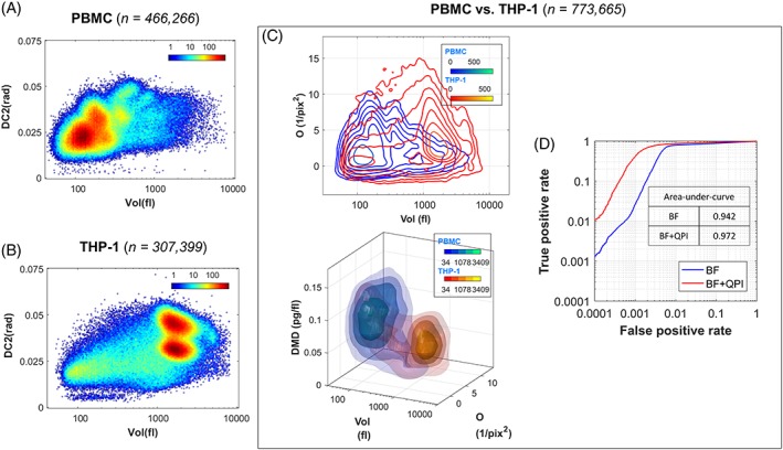
Ultra‐large‐scale label‐free multivariate classification of cancer cells and blood cells. Both (A) peripheral blood mononuclear cells (n = 466 266) and (B) leukemic monocytes (THP‐1, n = 307 399) show high degree of heterogeneity, as clearly revealed in the bivariate color‐coded density plots. (C) (Top) A contour (2D) map and (bottom) an iso‐surface (3D) map of the two cell types. (D) The receiver‐operating‐characteristic curves showing the label‐free classification accuracy. The significance of including quantitative phase imaging‐image‐derived features on classification accuracy is reflected by the increased area‐under‐curve

3. CONCLUSION

Based upon an ultrafast, interferometry‐free, phase‐gradient‐encoding concept, multi‐ATOM has an overall strength of enabling ultrahigh throughput QPI without compromising the subcellular resolution—a capability that is absent in both conventional camera‐based QPI and interferometric time‐stretch QPI. We demonstrated that multi‐ATOM, at least two orders‐of‐magnitude faster than the classical QPI approaches, can efficiently reconstruct individual subcellularly resolvable multicontrast, label‐free single‐cell images (both the phase, amplitude and DC images) within an enormous population (>700 000 cells). We showed that both ultrahigh imaging throughput and high label‐free subcellular content realized in multi‐ATOM critically enable high statistical discrimination power to classify leukemic cells and PBMCs. Such capability is generally challenging with current biophysical phenotyping techniques 4, 23, 33, 34. Therefore, this label‐free single‐cell imaging technique could find a new ground in many applications, especially when combined with the advanced high‐speed fluorescence single‐cell imaging 35, 36 for simultaneous biophysical and biochemical single‐cell phenotyping; or when integrated with image‐activated cell sorting for enabling downstream biomolecular analysis on targeted cells 37. It includes notably new cost‐effective liquid biopsy strategies, for example, and circulating tumor cell detection and prescreening, in which number of known biochemical markers and thus the bias and the cost of assay can be minimized; and new form of SCA in which the catalog of biophysical markers could complement and correlate the cellular heterogeneity information provided by the assays based on biochemical markers, and thus enable strategic cost‐effective ultra‐large‐scale SCA.

4. MATERIALS AND METHODS

4.1. Multi‐ATOM system configuration

The system consists of three functional modules (Figure 1A): (a) a time‐stretch module for wavelength‐time mapping, (b) a spectrally encoded imaging module for wavelength‐space mapping and (c) an asymmetric‐detection module for phase‐gradient encoding/decoding. In the time‐stretch module, a home‐built all‐normal dispersion laser (center wavelength = 1064 nm, bandwidth = 10 nm and repetition rate = 11.8 MHz) generates the pulse train (pulse width = ~12 ps), which is then stretched in time by a 10‐km single‐mode fiber (a total GVD = 1.78 ns/nm and 17 dB loss at 1064 nm [OFS, Norcross, Georgia]) and optically amplified by a ytterbium‐doped fiber amplifier module (output power = 36 dBm, on–off power gain = 36 dB)—resulting in an all‐optical wavelength‐swept source for multi‐ATOM. In the spectrally encoded imaging module, a diffraction grating (groove density = 1200/mm, Littrow angle = 42.3) spatially disperses the time‐stretched pulses to generate a one‐dimensional (1D) spectral shower. A pair of objective lenses (numerical aperture [NA] = 0.75 [front] and 0.8 [back]) forms a double‐pass configuration for imaging the suspended cells flowing in a custom‐designed microfluidic chip (flow rate > 1 m/s) along the orthogonal direction to the spectral shower. The same grating recombines the reflected image‐encoded spectral shower into a single collimated beam. Note that the local phase‐gradient induced by the imaged cells is spectrally encoded into intensity‐loss of each minimally resolvable point across the spectral shower. In the asymmetric‐detection module, a one‐to‐four demultiplexer splits the image‐encoded pulsed beam into four identical replicas, each of which is half‐blocked by a knife‐edge from four primary cardinal directions (ie, right, left, top and bottom) (Figure 1A,C). Then, the four beams are time‐multiplexed by the fiber delay lines and a fiber‐based four‐to‐one multiplexer. Hence, the four image‐encoded pulses (all correspond to the same line scan) are separated in time, that is, time‐multiplexed. A high‐speed single‐pixel photodetector (electrical bandwidth = 12 GHz [Newport, Irvine, California]) is used for continuous signal detection. For digitization, a real‐time FPGA‐based signal processing system is used (electrical bandwidth = 2 GHz, sampling rate = 4 GSa/s, throughput > 10 000 cell/s). Custom logic was implemented on the FPGA to automatically detect and segment cells from the digitized data stream in real time, at a processing throughput equivalent to >10 000 cell/s. This segmentation step is critical in maximizing the efficiency of the downstream data storage subsystem. All segmented cell images are sent through four 10G Ethernet links and are stored by four data‐receiving hosts with a total memory capacity of over 800 GB that can be extended easily.

4.2. Phase‐retrieval algorithm of multi‐ATOM

A key prerequisite of robust phase retrieval in multi‐ATOM is to create a temporally incoherent spectrally encoded line‐scanning illumination. Under this condition, which can be accomplished with high GVD, the propagation characteristics of each minimum spectrally resolvable beam across the line scan can adequately be modeled using geometrical ray‐tracing. This condition is satisfied when the time delay between the adjacent minimum spectrally resolvable spots τ _min is significantly greater than the effective coherence time τ _c (defined by the spectral resolution of the spectrally encoded illumination, δλ), that is, τ _min > > τ _c, where τ _min = δλ ∙ GVD and   τ_c = λ²/cδλ. c is the speed of light, and λ is the center wavelength of the light. Given that δλ = 0.2 nm, and GVD = 1.78 ns/nm employed in our system, the aforementioned condition is satisfied.

The central idea of phase retrieval of multi‐ATOM is integrating the phase gradients encoded in asymmetrically detected signal to obtain the quantitative phase image (ϕ(x, y)). In detail, two orthogonal phase‐gradient images (∇_xϕ(x, y) and ∇_yϕ(x, y)) are reconstructed from four asymmetrically detected intensity images (I_A(x, y), I_B(x, y), I_C(x, y) and I_D(x, y)—A, B, C, D in Figure 1) through three mapping equations: mapping from phase gradient to tilt angle of wavefront (Eq. (1)); mapping from tilt angle of wavefront to transverse beam translation (Eq. (2)); mapping from transverse beam translation to intensities of the four asymmetrically detected images (Eq. (3)). Throughout the derivation, the spatial coordinate of the image is indexed by symbols, x and y, and a flat beam profile (ie, Köhler illumination on the frontal plane in Figure S1) is considered for simplicity which can be approximated by overfilling the objective aperture.

A phase gradient presents when there is a spatial phase difference due to the refractive index mismatch and/or the thickness profile across phase objects, for example, biological cells. Consider a focused light beam illuminates on a phase object, refraction of light (ie, wavefront tilt) occurs because of the local phase gradient, as illustrated in Figure S1. In multi‐ATOM, this phenomenon applies to each minimally resolvable spectrally encoded beam along the spectral shower. Assuming the phase gradient is small and smooth across the phase object, one could apply the concept of ray optics to formulate the phase gradient, which is proportional to the tilt angle of wavefront under the paraxial approximation:

$$\left\{\begin{array}{c}{\nabla }_x\varphi \left(x,y\right)=2\pi {\theta }_x\left(x,y\right)/\lambda \\ {\nabla }_y\varphi \left(x,y\right)=2\pi {\theta }_y\left(x,y\right)/\lambda \end{array}\right.$$ (1)

where ∇_xϕ(x, y) and ∇_yϕ(x, y) are the phase gradients along the x and y directions; θ_x(x, y) and θ_y(x, y) are the tilt angles of wavefront along the x and y directions; λ is the center wavelength of light. The light tilt effectively leads to a transverse translation of the beam profile in the frontal plane. From the geometry of the light cone (transverse plane and sagittal plane in Figure S1), the translations (δL_x(x, y) and δL_y(x, y)) along the x and y directions can be related to the corresponding tilt angle of wavefront (θ_x and θ_y) by:

$$\left\{\begin{array}{c}\tan \left({\theta }_x\left(x,y\right)+{\theta }_{\mathrm{NA}}\right)=\left({\mathit{\delta L}}_x\left(x,y\right)+w/2\right)/f\\ \tan \left({\theta }_y\left(x,y\right)+{\theta }_{\mathrm{NA}}\right)=\left({\mathit{\delta L}}_y\left(x,y\right)+w/2\right)/f\end{array}\right.$$ (2)

where θ_NA and f are the acceptance angle and focal length of the objective lens, respectively. Here we assume the aperture in the frontal plane of the object to be a square with the sides of w. For simplicity, the two objective lenses are considered to have the same NA. The beam translation causes an incomplete light coupling to the back objective (or condenser lens) such that the power of coupled light decreases (frontal plane in Figure S1). In the current double‐pass configuration, the front objective lens also functions as the condenser lens—essentially leading to the same equal‐NA condition. Therefore, in practice, the NA of the two objective lenses are not necessarily to be identical, given that the NA of the back objective lens is higher than that of the front objective lens. Under this condition, the local light tilt and thus the phase gradient is effectively spectrally encoded into the power of each minimally resolvable beam across the spectral shower.

To decode the relative power loss due to the beam translations and thus the phase gradients along both the x and y directions, multiple intensity measurements of the same image are required. We adopt the asymmetric‐detection scheme that involves partial‐beam blocks on four beam replicas from the same line scan (Figure 1A). At each pixel coordinate (x, y), the relationship of the normalized intensity loss along the x and y directions (R_δx(x, y) and R_δy(x, y)), the intensities of these four image replicas (I_A(x, y), I_B(x, y), I_C(x, y) and I_D(x, y)) and the local beam translations (δL_x(x, y) and δL_y(x, y)) can be expressed by:

$$\left\{\begin{array}{c}{R}_{\mathit{\delta x}}\left(x,y\right)=\left(I_B\left(x,y\right)-I_A\left(x,y\right)\right)/2I_x\left(x,y\right)={\mathit{\delta L}}_x\left(x,y\right)/w\\ R_{\mathit{\delta y}}\left(x,y\right)=\left(I_C\left(x,y\right)-I_D\left(x,y\right)\right)/2I_y\left(x,y\right)={\mathit{\delta L}}_y\left(x,y\right)/w\end{array}\right.$$ (3)

where I_x(x, y) and I_y(x, y) are absorption‐contrast images along the x and y directions (Section 4 ).

By combining Eqns. 1, 2, 3, the two orthogonal phase gradients (∇_xϕ(x, y) and ∇_yϕ(x, y)) and thus the complex phase gradient (∇ϕ(x, y)) can be related to the measured intensity‐loss ratio along the x and y directions (R_δx(x, y) and R_δy(x, y)).

$$\left\{\begin{array}{c}{\nabla }_x\varphi \left(x,y\right)=2\pi \left({\tan }^{-1}\left(\left(2R_{\mathit{\delta x}}\left(x,y\right)+1\right)\tan \left({\theta }_{\mathrm{NA}}\right)\right)-{\theta }_{\mathrm{NA}}\right)/\lambda \\ {\nabla }_y\varphi \left(x,y\right)=2\pi \left({\tan }^{-1}\left(\left(2R_{\mathit{\delta y}}\left(x,y\right)+1\right)\tan \left({\theta }_{\mathrm{NA}}\right)\right)-{\theta }_{\mathrm{NA}}\right)/\lambda \\ \nabla \varphi \left(x,y\right)={\nabla }_x\varphi \left(x,y\right)+i{\nabla }_y\varphi \left(x,y\right)\end{array}\right.$$ (4)

Equation (4) indicates that in order to quantify the phase gradient and thus the phase, the only experimental quantity are the two normalized intensity losses (R_δx(x, y) and R_δy(x, y)). Specifically, they are the intensity ratios of the asymmetrically detected images along the x direction (ie, I_A(x, y) − I_B(x, y) ) and the y direction (ie, I_A(x, y) − I_B(x, y)) to its absorption‐contrast images (I_x(x, y) and I_y(x, y)) respectively (Section 4).

Complex Fourier integration is then applied on the phase gradient (∇ϕ(x, y)) to obtain the quantitative phase image (ϕ(x, y)),

$$\varphi \left(x,y\right)=\mathrm{CF}·\mathrm{Im}\left\{F^{-1}\left\{\mathrm{NF}·F\left\{\nabla \varphi \left(x,y\right)\right\}\right\}\right\}\text{where}\mathrm{NF}=\left\{\begin{array}{c}\mathrm{FOV}/\left(2\mathit{\pi i}·k\left(x,y\right)\right),k\left(x,y\right)\ne 0\\ 0,k\left(x,y\right)=0\end{array}\right.$$ (5)

where Im is the imaginary part of a complex number; F and F ⁻¹ are the forward and inverse Fourier transform operators, respectively; NF is a normalization factor for quantifying the phase and avoiding singularity in the integration operation; k(x,y) is the 2D wavenumbers; FOV is the 2D field‐of‐view; CF is the calibration factor for correcting the systematic phase deviation arise from nonideal system setting, i.e., Gaussian beam profile and circular aperture.

4.3. BF image reconstruction in multi‐ATOM

The four normalized asymmetrically detected images (I_A(x, y), I_B(x, y), I_C(x, y) and I_D(x, y)—A, B, C, D in Figure 1C) are divided into two sets of images based on their asymmetric‐detection orientations, that is, I_A(x, y) and I_B(x, y) as the horizontally blocked images, and I_C(x, y) and I_D(x, y) as the vertically blocked images. In each set, the intensity values of two images are compared pixel‐by‐pixel (ie, I_A(x, y) vs I_B(x, y) and I_C(x, y) vs I_D(x, y)) such that the pixels with maximum intensity from one of the two images are selected to form the absorption‐contrast image of each set (I_x(x, y) and I_y(x, y)).

$$\left\{\begin{array}{c}{I}_x\left(x,y\right)=\max \left\{I_A\left(x,y\right),I_B\left(x,y\right)\right\}\\ I_y\left(x,y\right)=\max \left\{I_C\left(x,y\right),I_D\left(x,y\right)\right\}\end{array}\right.$$ (6)

The BF image of a cell (BF(x, y)) is the sum of two resulting absorption contrasted images (I_x(x, y) and I_y(x, y)).

$$\mathrm{BF}\left(x,y\right)=I_x\left(x,y\right)+I_y\left(x,y\right)$$ (7)

From the above image reconstruction algorithm, the scattering loss caused by the cells would be minimized, such that the BF image would represent mostly the absorption loss.

4.4. Reconstruction of DC images

A DC image is transformed from a quantitative phase image through 2D convolution with a diffraction‐limited‐spot‐size kernel within which statistical SD of the phase value is calculated (Table S1). As a result, quantitative phases are transformed to DC values at each pixel. A binary mask obtained from the corresponding BF image is applied to the DC image to isolate the cell body from the whole image. A statistical histogram of DC of the cell is then generated from the masked DC image. The SD and the skewness, which corresponds to DC2 and DC3, respectively, are calculated from the histogram (Table S1).

4.5. Experimental configuration for performance comparison between iTM and multi‐ATOM

To compare the imaging performance between iTM and multi‐ATOM in a continuous data capturing scenario, we introduced two key modifications in the multi‐ATOM system (Figure 3A, S4, and Appendix S1). First, to capture both iTM and multi‐ATOM image data of the same cell simultaneously, an additional interferometry module was added. Specifically, a 50:50 beam splitter (Thorlabs, Newton, New Jersey) was placed right before the asymmetric‐detection module to equally split the beam into two replicas. One of the replicas entered the multi‐ATOM module; another entered the iTM module and was interfered with a reference beam (with the same power) using another 50:50 beam splitter which maximizes the interference fringe visibility. The resultant interferogram was detected by another single‐pixel photodetector (electrical bandwidth = 8.5 GHz, [Newport, Irvine, California]). Secondly, a real‐time oscilloscope with 4 times larger in detection bandwidth than the FPGA module (electrical bandwidth = 16.8 GHz, sampling rate = 80 GSa/s [Keysight, Santa Rosa, California]) was employed. Note that the real‐time high‐bandwidth oscilloscope was used here to ensure the raw data from both iTM (temporal interferogram) and multi‐ATOM (time‐multiplexed replica) were sufficiently oversampled such that diffraction‐limited resolution was achieved in both multi‐ATOM and iTM at the GVD given by the dispersive fiber available in the present work, that is, GVD = 1.78 ns/nm. The fringe density was configured (by tuning the reference arm length in the interferometer) to be sufficiently high to achieve the diffraction‐limited resolution and able to be resolved at the given GVD and sampling rate. These are the necessary conditions for fair comparison of image quality between multi‐ATOM and iTM. We note that in practice, the oscilloscope is incompatible with continuous cell image capture at high throughput because of its limited memory depth. The phase‐retrieval pipeline of iTM is detailed in Appendix S1. In brief, the iTM data are first downsampled to achieve the same GVD_eq condition prior to generation of the phase image. By applying a low‐pass filter on the 2D interferogram, we obtain a BF contrast image (Figure 3A). Finally, phase unwrapping, using Goldstein's branch cut algorithm based on the quality guided map, was applied to retrieve quantitative phase (Figure 3A). Note that this algorithm is chosen to maximize the phase‐retrieval yield, yet to avoid significant increase in the computational time 24).

4.6. Human PBMC isolation from human buffy coat

Human buffy coat was provided by the Hong Kong Red Cross, and all the blood donors have given written consent for clinical care and research purposes. The research protocol is approved by the Institutional Review Board at the University of Hong Kong. 2 mL of human buffy coat/fresh blood mixed well with 2 mL of phosphate‐buffed saline (PBS) and then carefully layered on top of 2 mL of Ficoll (GE Healthcare Life Sciences, Chicago, Illinois) inside a 10‐mL centrifuge tube without mixing. The centrifuge tube containing the above‐mentioned solutions was transferred to centrifugation under 400×g for 20 minutes after which the fluid is separated into five layers—corresponding to plasma, PBMCs, Ficoll, granulocytes and red blood cells (from top to bottom). PBMCs were carefully pipetted out from the corresponding layer and transferred to separated centrifuge tubes. The extracted PBMCs were then centrifuged and re‐suspended with 1× PBS to achieve cell count of ~10⁵ cells per mL.

4.7. Sample preparation of cell lines

Culture medium for THP‐1 (TIB‐202, ATCC, Manassas, Virginia), culturing was formulated with 90% Roswell Park Memorial Institute—1640 medium (Thermo Fisher Scientific, Waltham, Massachusetts), 10% fetal bovine serum and 1% 100× antibiotic‐antimycotic (Anti‐Anti; Thermo Fisher Scientific, Waltham, Massachusetts). Culture medium for MDA‐MB‐231 (HTB‐26; ATCC, Manassas, Virginia), and MCF‐7 (HTB‐22D; ATCC, Manassas, Virginia) culturing in Dulbecco's Modified Eagle Medium (DMED) (Gibco, Dun Laoghaire, Ireland) supplemented with 10% PBS and 1% 100× antibiotic‐antimycotic (Anti‐Anti; Thermo Fisher Scientific, Waltham, Massachusetts). Cells were cultured in a 5% CO₂ incubator under 37 °C and the medium was renewed twice a week. Cells were pipetted out adjusted to be around 10⁵ cells per mL of 1× PBS. Prevention of mycoplasma contamination was done by adding Antibiotic‐Antimycotic (Thermo Fisher Scientific, Waltham, Massachusetts) during cell culture. Cellular morphology was routinely checked during cell culture under the light microscope prior to imaging experiments.

CONFLICT OF INTEREST

We declare there is no conflict of interest in this work.

AUTHOR BIOGRAPHIES

Please see Supporting Information online.

Supporting information

Author Biographies

Appendix S1 Supporting Information

Lee KCM, Lau AKS, Tang AHL, et al. Multi‐ATOM: Ultrahigh‐throughput single‐cell quantitative phase imaging with subcellular resolution. J. Biophotonics. 2019;12:e201800479. 10.1002/jbio.201800479

REFERENCES

- 1. Majeed H., Sridharan S., Mir M., Ma L., Min E., Jung W., Popescu G., J. Biophotonics 2017, 10, 177. [DOI] [PubMed] [Google Scholar]
- 2. Park Y., Depeursinge C., Popescu G., Nat. Photonics 2018, 12, 578. [Google Scholar]
- 3. Popescu G., “Quantitative Phase Imaging of Cells and Tissues,” McGraw‐Hill professional, New York 2011. [Google Scholar]
- 4. Zangle T. A., Teitell M. A., Nat. Methods 2014, 11, 1221. [DOI] [PMC free article] [PubMed] [Google Scholar]
- 5. Girshovitz P., Shaked N. T., Biomed. Opt. Express 2012, 3, 1757. [DOI] [PMC free article] [PubMed] [Google Scholar]
- 6. Damania D., Subramanian H., Backman V., Anderson E. C., Wong M. H., OJ M. C., Phillips K. G., J. Biomed. Opt. 2014, 19, 016016. [DOI] [PMC free article] [PubMed] [Google Scholar]
- 7. Phillips K. G., Velasco C. R., Li J., Kolatkar A., Luttgen M., Bethel K., Duggan B., Kuhn P., OJ M. C., Front. Oncol. 2012, 2, 1. [DOI] [PMC free article] [PubMed] [Google Scholar]
- 8. Bishitz Y., Gabai H., Girshovitz P., Shaked N. T., J. Biophotonics 2014, 7, 624. [DOI] [PubMed] [Google Scholar]
- 9. Galler K., Bräutigam K., Bräutigam K., Große C., Popp J., Neugebauer U., Analyst 2014, 139, 1237. [DOI] [PubMed] [Google Scholar]
- 10. Proserpio V., Lönnberg T., Immunol. Cell Biol. 2016, 94, 225. [DOI] [PMC free article] [PubMed] [Google Scholar]
- 11. Lohmann A. W., Dorsch R. G., Mendlovic D., Ferreira C., Zalevsky Z., J. Opt. Soc. Am. A 1996, 13, 470. [DOI] [PubMed] [Google Scholar]
- 12. Jin D., Sung Y., Lue N., Kim Y.‐H., So P. T. C., Yaqoob Z., Cytom. Part A 2017, 91, 450. [DOI] [PMC free article] [PubMed] [Google Scholar]
- 13. Roitshtain D., Wolbromsky L., Bal E., Greenspan H., Satterwhite L. L., Shaked N. T., Cytom. Part A 2017, 91, 482. [DOI] [PubMed] [Google Scholar]
- 14. Gorthi S. S., Schonbrun E., Opt. Lett. 2012, 37, 707. [DOI] [PubMed] [Google Scholar]
- 15. Merola F., Memmolo P., Miccio L., Savoia R., Mugnano M., Fontana A., D'Ippolito G., Sardo A., Iolascon A., Gambale A., Ferraro P., Light Sci. Appl. 2017, 6, e16241. [DOI] [PMC free article] [PubMed] [Google Scholar]
- 16. Barteneva N. S. and Vorobjev I. A., Imaging Flow Cytometry Springer, New York 2016. [Google Scholar]
- 17. Lei C., Kobayashi H., Wu Y., Li M., Isozaki A., Yasumoto A., Mikami H., Ito T., Nitta N., Sugimura T., Yamada M., Yatomi Y., Di Carlo D., Ozeki Y., Goda K., Nat. Protoc. 2018, 13, 1. [DOI] [PubMed] [Google Scholar]
- 18. Goda K., Ayazi A., Gossett D. R., Sadasivam J., Lonappan C. K., Sollier E., Fard A. M., Hur S. C., Adam J., Murray C., Wang C., Brackbill N., di Carlo D., Jalali B., Proc. Natl. Acad. Sci. U S A 2012, 109, 11630. [DOI] [PMC free article] [PubMed] [Google Scholar]
- 19. Wong T. T. W. W., Lau A. K., Ho K. K., Tang M. Y., Robles J. D., Wei X., Chan A. C., Tang A. H., Lam E. Y., Wong K. K., Chan G. C., Shum H. C., Tsia K. K., Sci. Rep. 2014, 4, 1. [DOI] [PMC free article] [PubMed] [Google Scholar]
- 20. Lau A. K. S., Shum H. C., Wong K. K. Y., Tsia K. K., Lab Chip 2016, 16, 1743. [DOI] [PubMed] [Google Scholar]
- 21. Goda K., Tsia K. K., Jalali B., Nature 2009, 458, 1145. [DOI] [PubMed] [Google Scholar]
- 22. Guo B., Lei C., Wu Y., Kobayashi H., Ito T., Yalikun Y., Lee S., Isozaki A., Li M., Jiang Y., Yasumoto A., di Carlo D., Tanaka Y., Yatomi Y., Ozeki Y., Goda K., Methods 2018, 136, 116. [DOI] [PubMed] [Google Scholar]
- 23. Chen C. L., Mahjoubfar A., Tai L.‐C., Blaby I. K., Huang A., Niazi K. R., Jalali B., Sci. Rep. 2016, 6, 1. [DOI] [PMC free article] [PubMed] [Google Scholar]
- 24.A.K. Lau, T.T.W. Wong, K.K. Ho, M.Y.H. Tang, A.C.S. Chan, X. Wei, E.Y. Lam, H.C. Shum, K.K.Y. Wong, K.K. Tsia, J. Biomed. Opt. 2014, 19, 076001. [DOI] [PubMed] [Google Scholar]
- 25. Tsia K. K., Goda K., Capewell D., Jalali B., Opt. Express 2010, 18, 10016. [DOI] [PubMed] [Google Scholar]
- 26. Guo B., Lei C., Kobayashi H., Ito T., Yalikun Y., Jiang Y., Tanaka Y., Ozeki Y., Goda K., Cytom. Part A 2017, 91, 494. [DOI] [PubMed] [Google Scholar]
- 27. Tang A. H. L., QTK L., BMF C., KCM L., ATY M., Yip G. K., AHC S., KKY W., Tsia K. K., J. Vis. Exp. 2017, 124, 1. [Google Scholar]
- 28. Chan A. C. S., Ng H. C., Bogaraju S. C. V., So H. K. H., Lam E. Y., Tsia K. K., Sci. Rep. 2017, 7, 1. [DOI] [PMC free article] [PubMed] [Google Scholar]
- 29. Goda K., Solli D. R., Tsia K. K., Jalali B., Phys. Rev. A 2009, 80, 043821. [Google Scholar]
- 30. Guiglia D. and Pritt M., “Two‐Dimensional Phase Unwrapping: Theory, Algorithm, and Software,” Wiley, Hoboken 1998. [Google Scholar]
- 31. Goldstein R. M., Zebker H. A., Werner C. L., Radio Sci. 1988, 23, 713. [Google Scholar]
- 32. Fang S., Meng L., Wang L., Yang P., Komori M., Appl. Opt. 2011, 50, 5446. [DOI] [PubMed] [Google Scholar]
- 33. Holliday D. L., Speirs V., Breast Cancer Res. 2011, 13, 1. [DOI] [PMC free article] [PubMed] [Google Scholar]
- 34. Tse H. T. K., Gossett D. R., Moon Y. S., Masaeli M., Sohsman M., Ying Y., Mislick K., Adams R. P., Rao J., Di Carlo D., Sci. Transl. Med. 2013, 5, 212ra163. [DOI] [PubMed] [Google Scholar]
- 35. Wu J., AHL T., ATY M., Yan W., GCF C., KKY W., Tsia K. K., Biomed. Opt. Express 2017, 8, 4160. [DOI] [PMC free article] [PubMed] [Google Scholar]
- 36. Yan W., Wu J., Wong K. K. Y., Tsia K. K., J. Biophotonics 2018, 11, 1. [DOI] [PubMed] [Google Scholar]
- 37. Nitta N., Sugimura T., Isozaki A., Mikami H., Hiraki K., Sakuma S., Iino T., Arai F., Endo T., Fujiwaki Y., Fukuzawa H., Hase M., Hayakawa T., Hiramatsu K., Hoshino Y., Inaba M., Ito T., Karakawa H., Kasai Y., Koizumi K., Lee S., Lei C., Li M., Maeno T., Matsusaka S., Murakami D., Nakagawa A., Oguchi Y., Oikawa M., Ota T., Shiba K., Shintaku H., Shirasaki Y., Suga K., Suzuki Y., Suzuki N., Tanaka Y., Tezuka H., Toyokawa C., Yalikun Y., Yamada M., Yamagishi M., Yamano T., Yasumoto A., Yatomi Y., Yazawa M., Di Carlo D., Hosokawa Y., Uemura S., Ozeki Y., Goda K., Cell 2018, 175(1), 266–276. [DOI] [PubMed] [Google Scholar]
Associated Data
This section collects any data citations, data availability statements, or supplementary materials included in this article.
Supplementary Materials