Reconstructing High-Quality Diffusion MRI Data from Orthogonal Slice-Undersampled Data Using Graph Convolutional Neural Networks

Abstract

Diffusion MRI (dMRI), while powerful for the characterization of tissue microstructure, suffers from long acquisition times. In this paper, we propose a super-resolution (SR) reconstruction method based on orthogonal slice-undersampling for accelerated dMRI acquisition. Instead of scanning full diffusion-weighted (DW) image volumes, only a subsample of equally-spaced slices need to be acquired. We show that complementary information from DW volumes corresponding to different diffusion wave-vectors can be harnessed using graph convolutional neural networks for reconstruction of the full DW volumes. We demonstrate that our SR reconstruction method outperforms typical interpolation methods and mitigates partial volume effects. Experimental results indicate that acceleration up to a factor of 5 can be achieved with minimal information loss.

1. Introduction

Diffusion MRI (dMRI) is a unique imaging technique for investigating tissue microstructural properties in vivo and non-invasively. However, in contrast to structural MRI, dMRI typically requires longer acquisition times for sufficient coverage of the diffusion wave-vector space (i.e., q-space). Each point in q-space corresponds to a diffusion-weighted (DW) image, and a sufficient number of DW images are typically required for accurate characterization of the white matter neuronal architecture, such as fiber crossings and intra-/extra-cellular compartments [1,2]. To accelerate acquisition while preserving the resolution in the wave-vector space, we introduce in this paper a super-resolution (SR) reconstruction technique that only requires a subsample of slices for each DW volume.

In this paper, we will introduce an SR reconstruction method for multifold acceleration of dMRI. We will show that, for each DW volume, only a subsample of slices in slice-select directions are needed to reconstruct the full 3D volumes, yielding an acceleration factor that is proportional to the subsampling factor. Each DW volume is subsampled with a different slice offset so that the volume captures complementary information that can be used to improve the reconstruction of the other DW volumes. Instead of limiting the slice-undersampling in one direction, we propose an orthogonal slice-undersampling scheme for increasing complementary information between undersampled DW volumes. In contrast to collecting multiple orthogonal scans as proposed in [3], our approach acquires a single DW image for each wave-vector, and hence does not prolong the acquisition time.

A non-linear mapping from the undersampled to the full DW images is learned using a graph convolutional neural network (GCNN) [4], which generalizes CNNs to high-dimensional and non-Euclidean domains. Such generalization is necessary in our framework since sampling in the q-space is not necessarily Cartesian. We fully exploit the relationships of neighboring sampling points in the spatial domain and the diffusion wave-vector domain in the form of a graph. To learn the target images with improved perceptual quality, the GCNN is employed as the generator in a generative adversarial network (GAN) [5]. GANs have been shown to yield impressive performance in natural image generation and translation [6].

2. Methods

2.1. Formulation

Each of the N DW volumes {X_n, n = 1, … ,N} is undersampled in the slice-select direction by a factor of R:

$${\tilde{X}}_n\left(x,y,z\right):=\{\begin{array}{l}{X}_n\left(x,y,Rz+s_n\right),\\ X_n\left(x,Ry+s_n,z\right),\\ X_n\left(Rx+s_n,y,z\right),\end{array}\begin{array}{l}\text{for}\text{axial}\text{scan},\\ \text{for}\text{coronal}\text{scan},\\ \text{for}\text{sagittal}\text{sacn},\end{array}$$ (1)

where s_n ϵ {0, 1, … ,R − 1} is a slice offset for X_n in each scan direction. Our objective is to reconstruct the full DW volumes from the undersampled data by learning a non-linear mapping function f such that

$$\left(X_1,\cdots ,X_N\right)=f\left({\tilde{X}}_1,\cdots ,{\tilde{X}}_N\right).$$ (2)

In the current work, the mapping function is learned using GCNN.

An overview of the proposed method is illustrated in Fig. 1. First, the set of wave-vectors is divided into three subsets, with each subset associated to a scan direct (axial, coronal, or sagittal) and corresponding to a set of uniformly distributed gradient vectors. Since the graph for each scan direction can be different, GCNN is applied separately for each scan direction. Refinement layers are applied to generate the final DW volumes by considering the correlation across scan directions.

Fig. 1.

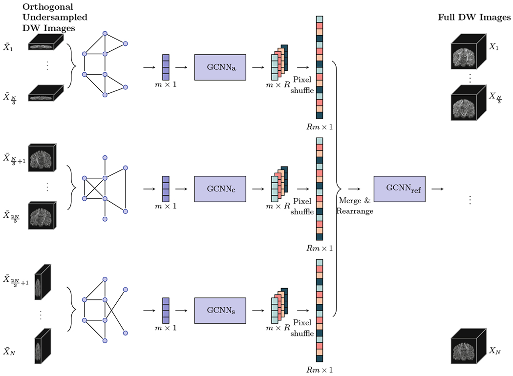
Method Overview: GCNN_a, GCNN_c, and GCNN_s denote the GCNNs for the axial, coronal, and sagittal scan directions, respectively. GCNN_ref denotes the GCNN for refinement.

2.2. Graph Representation and Spectral Filtering

The dMRI sampling domain can be represented by a graph where each node represents a physical spatial location in x-space and a diffusion wave-vector in q-space. This graph is encoded using an adjacency matrix W and the graph Laplacian is defined as L = D – W, where D is a diagonal degree matrix. L can be normalized via L = I – D^−1/2WD^−1/2, where I is an identity matrix. In this work, we define the adjacency matrix W considering spatio-angular neighborhoods as in [7].

Since a localized filter in the spatial domain should be smooth in the spectral domain, localized filters can be approximated and parameterized by polynomials [4]. Spectral filters approximated by the K-th order polynomials of the Laplacian are exactly K-localized in the graph [8]. In this work, we employ the Chebyshev polynomial approximation and define the graph convolutional operation from input x to output y as $y={\sum }_{k=0}^K{\theta }_k{T}_k\left(\tilde{L}\right)x,$ where $\tilde{L}$ is the scaled Laplacian $\tilde{L}=2L/{\lambda }_{\max }-I$ with λ_max being the maximal eigenvalue of L, and T_k(·) is the Chebyshev polynomial of order k. Then, the graph convolutional layers in the GCNN can be represented as

$${\mathbf{\Phi }}^{\left(l\right)}=\xi \left(\sum _{k=0}^K{\Theta }_k^{\left(l\right)}{T}_k\left(\tilde{L}\right){\mathbf{\Phi }}^{\left(l-1\right)}\right),$$ (3)

where Φ^(l) denotes the feature map at the l-th layer, ${\Theta }_k^{\left(l\right)}$ is a matrix of Chebyshev polynomial coefficients to be learned at the l-th layer, and ξ is a non-linear activation function.

2.3. Graph Convolutional Neural Networks

Based on the graph convolutional operation, a residual convolutional block [9] and U-Net [10] structure with encoding and decoding are employed. Pooling and unpooling, realized using graph coarsening and uncoarsening, are applied respectively for each encoding and decoding step. As in [4], we adopt the Graclus multi-scale clustering algorithm [11] for graph coarsening. The diffusion signals corresponding to the nodes of the graph are rearranged via index permutation to form a vector. The uncoarsening operation is achieved via a one-dimensional upsampling operation followed by an inverse permutation of indices. Multi-scale graphs, obtained via graph coarsening, are fed as features via graph convolutions to each level of the encoding path. The skip connection at each level in the U-Net consists of a transformation module (graph convolutions and concatenation) for boosting the low-level features to complement the high-level features, as proposed in [12]. The transformation module narrows the gap between low- and high-level features.

The upsampling operation in slice-select direction is realized by a standard convolution in the low-resolution space followed by pixel shuffling [13]. The pixelshuffling operation maps R feature maps of size m × 1 to an output of size Rm × 1, where m is the number of nodes in the input graph and R is the desired upsampling factor.

In the decoding path, inspired by [14], we add a branch to compute diffusion indices such as generalized fractional anisotropy (GFA) [15]. This branch provides the microstructure estimation of dMRI data and can help the generator to produce dMRI data with more accurate diffusion indices. In this work, we focus on only GFA which is estimated by two consecutive fully-connected layers.

The proposed architecture for each scan direction is illustrated in Fig. 2. For the refinement network, we apply graph convolutional layer followed by two consecutive residual convolutional blocks. The final output is obtained via a graph convolution layer with one output channel.

Fig. 2.

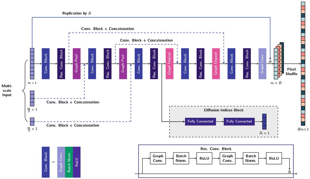
The proposed graph CNN architecture for GCNN_a, GCNN_c and GCNN_s. The number of feature maps is set to 64 for all layers except for the last graph convolutional layer, which has R channels for each scan direction.

2.4. Loss Function

We employ the adversarial learning strategy to match the distribution of the generated images to the distribution of target images. For the input source x, the target DW image y, and the target GFA y_GFA , the generator loss is defined as the combination of pixel-wise difference, GFA difference, and adversarial loss:

$${\mathcal{L}}_G\left(\mathbf{x},\mathbf{y},{\mathbf{y}}_{\text{GFA}}\right)={\lambda }_I{\Vert G_I\left(\mathbf{x}\right)-\mathbf{y}\Vert }_1+{\lambda }_{\text{GFA}}{\Vert G_{\text{GFA}}\left(\mathbf{x}\right)-{\mathbf{y}}_{\text{GFA}}\Vert }_1+{\lambda }_{\text{ADV}}{\mathcal{L}}_{\text{BCE}}\left(D_I\left(G_I\left(\mathbf{x}\right)\right),\mathbf{1}\right)+{\lambda }_{\text{ADV}}{\mathcal{L}}_{\text{BCE}}\left(D_{\text{GFA}}\left(G_{\text{GFA}}\left(\mathbf{x}\right)\right),\mathbf{1}\right),$$ (4)

where ${\mathcal{L}}_{\mathrm{BCE}}$ is the binary cross-entropy function. In (4), G_I(x) and G_GFA(x) are the outputs of the generator in the reconstruction path and diffusion index path, respectively. We define the discriminator loss as

$${\mathcal{L}}_{D_I}\left(\mathbf{x},\mathbf{y}\right)={\mathcal{L}}_{\text{BCE}}\left(D_I\left(\mathbf{y}\right),\mathbf{1}\right)+{\mathcal{L}}_{\text{BCE}}\left(D_I\left(G_I\left(\mathbf{x}\right)\right),\mathbf{0}\right),$$ (5)

$${\mathcal{L}}_{D_{\text{GFA}}}\left(\mathbf{x},{\mathbf{y}}_{\text{GFA}}\right)={\mathcal{L}}_{\text{BCE}}\left(D_{\text{GFA}}\left({\mathbf{y}}_{\text{GFA}}\right),\mathbf{1}\right)+{\mathcal{L}}_{\text{BCE}}\left(D_{\text{GFA}}\left(G_{\text{GFA}}\left(\mathbf{x}\right)\right),\mathbf{0}\right),$$ (6)

where D_I and D_GFA are the discriminators for the predicted images and GFA, respectively. D_I is based on patch-GAN [6] which consists of three graph convolutions with 64, 128, 256 features, each followed by leaky ReLU (LReLU) and graph pooling. D_GFA consists of three fully-connected layers with 64, 32, and 1 node(s), respectively.

3. Experimental Results

3.1. Material and Implementation Details

We randomly selected 16 subjects from the Human Connectome Project (HCP) database [16] and divided them into 12 for training and 4 for testing for 4-fold cross-validation. For each subject, 90 DW images (voxel size: 1.25 × 1.25 × 1.25mm³) with b = 2000s/mm² were used for evaluation. The images were retrospectively undersampled by factors R = 3,4, and 5. After being divided into three subsets for different scan directions, each subset was further divided into R groups, where the wave-vectors were uniformly distributed in each group. For each group, the source images were generated by undersampling the original images with a slice offset based on its scan direction. Practically, such an undersampling scheme can be implemented by scanning only a selective set of slices for each point in the q-space. All DW images were normalized by their corresponding non-DW image (b₀). The order K for the Chebyshev polynomials is set to 3. For the loss functions, we set λ_I = 1.0, λ_GFA = 0.1, and λ_ADV = 0.01. The proposed method was implemented using TensorFlow 1.12.0 and trained with the ADAM optimizer with an initial learning rate of 0.0001 and 0.00001 for the generator and the discriminator, respectively.

3.2. Results

We compared our SR method with two conventional methods: Bicubic interpolation and 3D U-Net [17] applied to input images upsampled with bicubic interpolation. Three different undersampling factors R = 3, 4, and 5 are considered. The number of channels for 3D U-Net is set so that its number of training parameters is comparable to the proposed method. We measured the reconstruction accuracy of the reconstructed dMRI data by mean absolute error (MAE), peak signal-to-noise ratio (PSNR), and structural similarity index (SSIM). Quantitative results are summarized in Fig. 3.

Fig. 3.

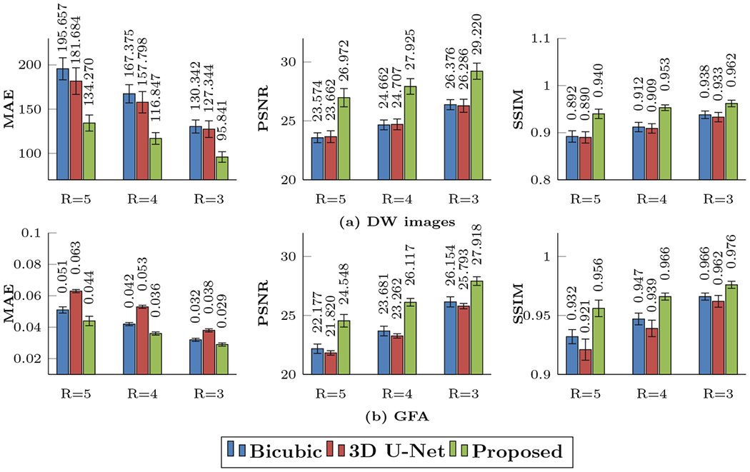
Quantitative comparison using MAE, PSNR, and SSIM of (a) DW images and (b) GFA maps.

Representative results for GFA images computed from the reconstructed full DW images at a fixed undersampling factor R = 4, shown in Fig. 4, indicate that the proposed method recovers more structural details compared with the two conventional methods which exploit only spatial correlation. Figure 5 shows that our method can yield fiber orientation distribution functions (ODFs) that are closer to the ground truth with less partial volume effects, especially in regions marked by rectangles.

Fig. 4.

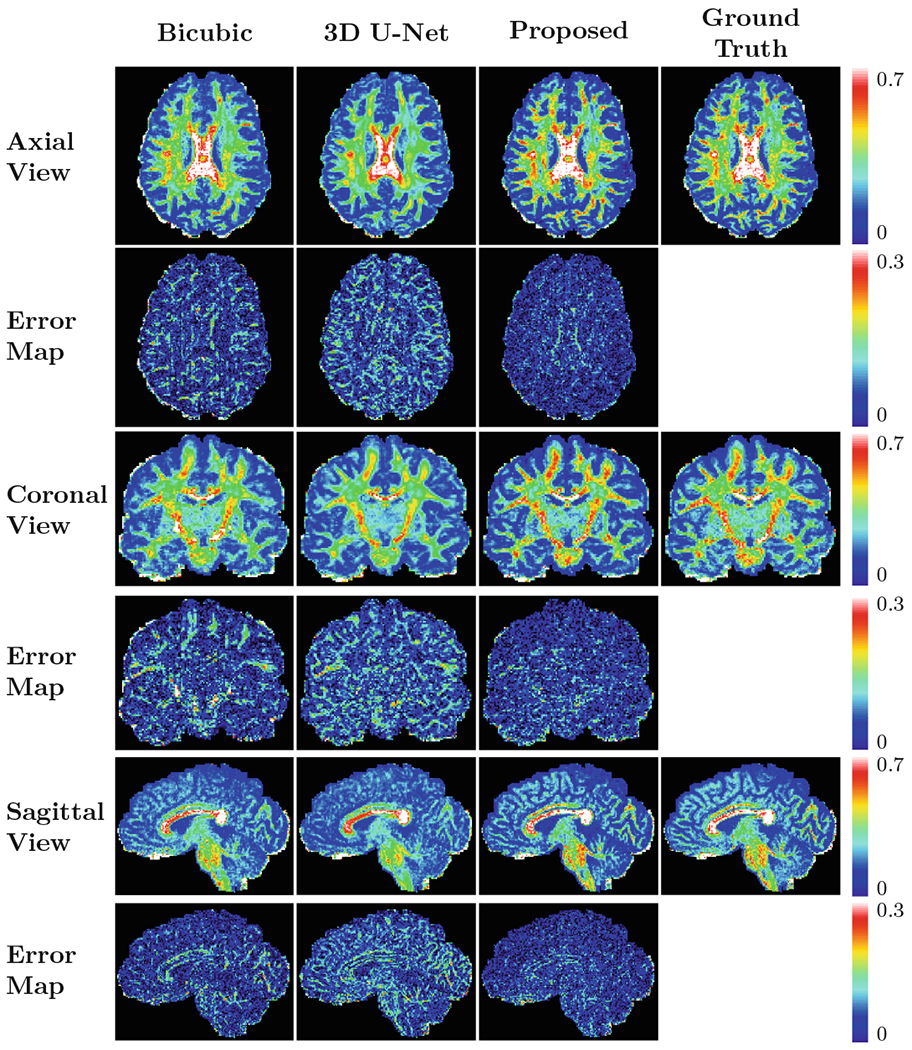
Predicted GFA maps and the corresponding error maps shown in multiple views (R = 4).

Fig. 5.

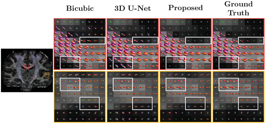
Representative fiber ODFs (R = 4).

4. Conclusion

We have proposed to employ orthogonal slice-undersampling for acceleration of dMRI. Each DW image is undersampled with a different slice offset, and the full DW images are reconstructed by exploiting neighborhood information in the spatial and angular domains. The non-linear mapping from slice-undersampled DW images to the full DW images is learned using GCNN. The spatio-angular relationship is jointly considered when constructing the graph for the GCNN. The experimental results demonstrate that the proposed method outperforms the commonly-used interpolation method and a 3D U-Net based SR reconstruction method.

References

- 1.Yap PT, Zhang Y, Shen D: Multi-tissue decomposition of diffusion MRI signals via l0 sparse-group estimation. IEEE Trans. Image Process 25(9), 4340–4353 (2016) [DOI] [PMC free article] [PubMed] [Google Scholar]
- 2.Ye C, Zhuo J, Gullapalli RP, Prince JL: Estimation of fiber orientations using neighborhood information. Med. Image Anal 32, 243–256 (2016) [DOI] [PMC free article] [PubMed] [Google Scholar]
- 3.Scherrer B, Gholipour A, Warfield SK: Super-resolution reconstruction to increase the spatial resolution of diffusion weighted images from orthogonal anisotropic acquisitions. Med. Image Anal 16(7), 1465–1476 (2012) [DOI] [PMC free article] [PubMed] [Google Scholar]
- 4.Defferrard M, Bresson X, Vandergheynst P: Convolutional neural networks on graphs with fast localized spectral filtering In: Advances in Neural Information Processing Systems (NIPS), pp. 3844–3852 (2016) [Google Scholar]
- 5.Goodfellow I, et al. : Generative adversarial nets In: Advances in Neural Information Processing Systems (NIPS), pp. 2672–2680 (2014) [Google Scholar]
- 6.Isola P, Zhu JY, Zhou T, Efros AA: Image-to-image translation with conditional adversarial networks. arXiv preprint (2017) [Google Scholar]
- 7.Chen G, Dong B, Zhang Y, Shen D, Yap P-T: Neighborhood matching for curved domains with application to denoising in diffusion MRI In: Descoteaux M, Maier-Hein L, Franz A, Jannin P, Collins DL, Duchesne S (eds.) MICCAI 2017. LNCS, vol. 10433, pp. 629–637. Springer, Cham: (2017). 10.1007/978-3-319-66182-7.72 [DOI] [PMC free article] [PubMed] [Google Scholar]
- 8.Hammond DK, Vandergheynst P, Gribonval R: Wavelets on graphs via spectral graph theory. Appl. Comput. Harmon. Anal 30(2), 129–150 (2011) [Google Scholar]
- 9.He K, Zhang X, Ren S, Sun J: Deep residual learning for image recognition. In: Computer Vision and Pattern Recognition (CVPR), pp. 770–778 (2016) [Google Scholar]
- 10.Ronneberger O, Fischer P, Brox T: U-Net: convolutional networks for biomedical image segmentation In: Navab N, Hornegger J, Wells WM, Frangi AF (eds.) MICCAI 2015. LNCS, vol. 9351, pp. 234–241. Springer, Cham: (2015). 10.1007/978-3-319-24574-4_28 [DOI] [Google Scholar]
- 11.Dhillon IS, Guan Y, Kulis B: Weighted graph cuts without eigenvectors a multilevel approach. IEEE Trans. Pattern Anal. Mach. Intell 29(11), 1944–1957 (2007) [DOI] [PubMed] [Google Scholar]
- 12.Nie D, Wang L, Adeli E, Lao C, Lin W, Shen D: 3-D fully convolutional networks for multimodal isointense infant brain image segmentation. IEEE Trans. Cybern 49(3), 1123–1136 (2018) [DOI] [PMC free article] [PubMed] [Google Scholar]
- 13.Shi W, et al. : Real-time single image and video super-resolution using an efficient sub-pixel convolutional neural network In: Computer Vision and Pattern Recognition (CVPR), pp. 1874–1883 (2016) [Google Scholar]
- 14.Chen G, Hong Y, Huynh K, Lin W, Shen D, Yap PT: Prediction of multi-shell diffusion MRI data using deep neural networks with diffusion loss. In: 105th RSNA Scientific Assembly and Annual Meeting (2019) [Google Scholar]
- 15.Tuch DS: Q-ball imaging. Magn. Reson. Med 52(6), 1358–1372 (2004) [DOI] [PubMed] [Google Scholar]
- 16.Sotiropoulos SN, et al. : Advances in diffusion MRI acquisition and processing in the human connectome project. NeuroImage 80, 125–143 (2013) [DOI] [PMC free article] [PubMed] [Google Scholar]
- 17.Çiçek Ö, Abdulkadir A, Lienkamp SS, Brox T, Ronneberger O: 3D U-Net: learning dense volumetric segmentation from sparse annotation In: Ourselin S, Joskowicz L, Sabuncu MR, Unal G, Wells W (eds.) MICCAI 2016. LNCS, vol. 9901, pp. 424–432. Springer, Cham: (2016). 10.1007/978-3-319-46723-8_49 [DOI] [Google Scholar]