Multifold Acceleration of Diffusion MRI via Deep Learning Reconstruction from Slice-Undersampled Data

Abstract

Diffusion MRI (dMRI), while powerful for characterization of tissue microstructure, suffers from long acquisition time. In this paper, we present a method for effective diffusion MRI reconstruction from slice-undersampled data. Instead of full diffusion-weighted (DW) image volumes, only a subsample of equally-spaced slices need to be acquired. We show that complementary information from DW volumes corresponding to different diffusion wavevectors can be harnessed using graph convolutional neural networks for reconstruction of the full DW volumes. The experimental results indicate a high acceleration factor of up to 5 can be achieved with minimal information loss.

1. Introduction

Diffusion MRI (dMRI) is a unique imaging technique for in vivo measurement of tissue microstructural properties. However, in contrast to structural MRI, dMRI typically requires longer acquisition times for sufficient coverage of the diffusion wavevector space (i.e., q-space). Each point in q-space corresponds to a diffusion-weighted (DW) image, and sufficient DW images are typically required for accurate characterization of the white matter neuronal architecture, such as fiber crossings and intra-/extra-cellular compartments [16,26,27]. To improve acquisition speed, we introduce in this paper a super-resolution (SR) reconstruction technique that only requires a subsample of slices for each DW volume.

In-plane and through-plane resolutions are determined by different factors. The former is affected by gradient strength, receiver bandwidth, phase encoding steps, and the number of readout points. The latter is determined by hardware limitations coupled with pulse sequence timing, and slice selection [8]. Fast and high-resolution reconstruction schemes can be designed by customizing MR acquisition and reconstruction. For example, SR reconstruction can be carried out with sub-voxel shifted scans in the in-plane [18] and slice-select [8] dimensions. Scherrer and his colleagues [21] proposed an SR method to reconstruct each DW volume from multiple anisotropic orthogonal scans, which they extended in [20] for estimation of tissue microstructural properties using diffusion compartment imaging. Ning et al. [17] proposed a compressed-sensing SR reconstruction framework that increases the spatio-angular resolution of dMRI data by using multiple overlapping thick-slice datasets with undersampling in q-space [17]. In [25], high-resolution diffusion parameters are estimated from a set of DW images with arbitrary slice orientation and diffusion gradient directions. Shi et al. [22] proposed a 4D low-rank and total variation regularized method for SR reconstruction. SR reconstruction based on a generative adversarial network is proposed in [1].

In this paper, we will introduce an SR reconstruction method for multifold acceleration of dMRI. We will show that, for each DW volume, only a subsample of slices in the slice select direction are needed to reconstruct the full 3D volumes, yielding an acceleration factor that is proportional to the subsampling factor. Each DW volume is subsampled with a different slice offset so that the volume captures complementary information that can be used to improve the reconstruction of other DW volumes. The non-linear mapping from the subsampled to full DW images is learned using a graph convolutional neural network (GCNN) [3,11], which generalizes CNNs to high-dimensional, irregular, and non-Euclidean domains. Such generalization is necessary in our framework since the sampling points in the q-space are not necessarily Cartesian. For improving perceptual quality, the GCNN is employed as the generator in a generative adversarial network (GAN) [7].

2. Methods

2.1. Formulation

A method overview is illustrated in Fig. 1. Each of the N DW volumes {X_n, n = 1, ⋯ , N} is undersampled in the slice-select direction by a factor of R:

$${\tilde{X}}_n\left(\cdot ,\cdot ,z\right):=X_n\left(\cdot ,\cdot ,Rz+s_n\right),$$ (1)

where s_n ∈ {0, 1, ⋯ , R − 1} is the slice offset for X_n. Our objective is to predict the full DW volumes from the undersampled data by learning a non-linear mapping function f such that

$$\left(X_1,\cdots ,X_N\right)=f\left({\tilde{X}}_1,\cdots ,{\tilde{X}}_N\right).$$ (2)

Instead of reconstructing each DW volume individually, we reconstruct all DW volumes jointly by considering neighborhoods in the spatial and diffusion wavevector domains. The mapping function in (2) f is learned using GCNN.

Fig. 1.

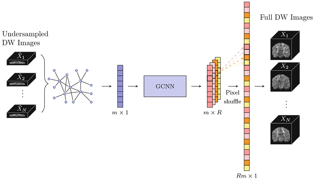
Method overview.

2.2. Graph Representation

The dMRI sampling domain can be represented by a graph where each node represents a spatial location in physical space (x-space) and a diffusion wave-vector in q-space. This graph is encoded using a weighted symmetric adjacency matrix W. The graph Laplacian is defined as L = D − W, where D is a diagonal degree matrix. L can be normalized via L = I − D^−1/2WD^−1/2, where I is an identity matrix. The eigenvectors of L define a graph Fourier basis that allows filtering to be performed in the spectral domain [5].

2.3. Spectral Filtering

According to Parseval’s theorem [2], a filter is localized in the spatial domain if and only if it is smooth in the spectral domain [3]. This can be achieved by approximating and parameterizing filters by polynomials [2]. Spectral filters approximated by the K-th order polynomials of the Laplacian are exactly K-localized in the graph [9]. In this work, we employ the Chebyshev polynomial approximation and define the graph convolutional operation from input x to output y as

$$y=g_{\theta }\left(x\right)=\sum _{k=0}^K{\theta }_k{T}_k\left(\tilde{L}\right)x,$$ (3)

where $\tilde{L}$ is the scaled Laplacian $\tilde{L}=2L/{\lambda }_{\max }-I$ with λ_max being the maximal eigenvalue of L and T_k(·) is the Chebyshev polynomial of order k. Chebyshev polynomials {T_k(·)} form an orthogonal basis on [−1, 1] and have recurrence relation

$$T_k\left(\lambda \right)=2\lambda T_{k-1}\left(\lambda \right)-T_{k-2}\left(\lambda \right),T_1\left(\lambda \right)=\lambda ,T_0\left(\lambda \right)=1.$$ (4)

The graph convolutional layers in the GCNN can be written as

$${\mathbf{\Phi }}^{\left(l\right)}=\xi \left(\sum _{k=0}^K{\theta }_k^{\left(l\right)}{T}_k\left(\tilde{L}\right){\mathbf{\Phi }}^{\left(l-1\right)}\right),$$ (5)

where Φ^(l) denotes the feature map at the l-th layer, ${\theta }_k^{\left(l\right)}$ is a vector of Chebyshev polynomial coefficients to be learned at the l-th layer, and ξ is a non-linear activation function.

2.4. Adjacency Matrix

The adjacency matrix is defined by considering spatio-angular neighborhoods. Let each node be represented by a spatial location ${\mathbf{x}}_i\in {\mathbb{R}}^3$ and a normalized wave-vector ${\mathbf{g}}_j\in {\mathbb{R}}^3$. Inspired by the local neighborhood matching technique [4], we define an adjacency matrix W with weights {w_{i,j;i′,j′}}:

$$w_{i,j,i^{\prime },j^{\prime }}:=\exp \left(-\frac{{\Vert {\mathbf{x}}_i-{\mathbf{x}}_{i^{\prime }}\Vert }_2^2}{{\sigma }_x^2}\right)\exp \left(-\frac{1-{\langle {\mathbf{g}}_j,{\mathbf{g}}_{j^{\prime }}\rangle }^2}{{\sigma }_g^2}\right),$$ (6)

where σ_x and σ_g are the parameters used to control the contributions of the spatial and angular distances, respectively. We note that, in (6), the numerators of the arguments of the exponential functions are normalized to [0, 1].

2.5. Graph Convolutional Neural Networks

The proposed architecture is illustrated in Fig. 2. A residual convolutional block is employed to ease training since it can mitigate the vanishing gradient problem [10]. To increase the receptive field, a U-Net [19] structure with symmetric contraction paths for encoding and expansion paths for decoding is employed. Pooling and unpooling, realized using graph coarsening and uncoarsening, are applied respectively for each encoding and decoding step. As in [5], we adopt the Graclus multi-scale clustering algorithm [6] for graph coarsening. The diffusion signals corresponding to the nodes of the graph are rearranged via index permutation to form a vector. The uncoarsening operation is achieved via a one-dimensional upsampling operation followed by an inverse permutation of indices. We employ the transposed convolution filter [13] for upsampling.

Fig. 2.

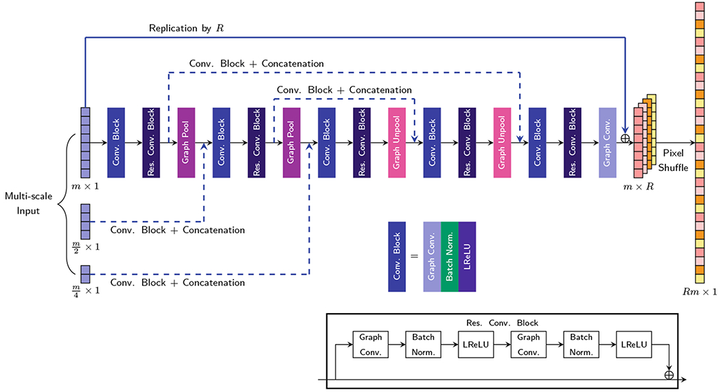
The proposed graph CNN architecture.

Multi-scale graphs, obtained via graph coarsening, are fed as features via graph convolutions to each level of the contraction path. The skip connection at each level in the U-Net consists of a transformation module (graph convolutions and concatenation) for boosting the low-level features to complement the high-level features, as proposed in [15]. The transformation model narrows the gap between low- and high-level features.

The upsampling operation in slice direction is realized by a standard convolution in the low-resolution space followed by pixel shuffling [23]. The pixel-shuffling operation maps R feature maps of size m×1 to an output of size Rm×1, where m is the number of nodes in the input graph.

2.6. Adversarial Learning

We employ the adversarial learning for better perceptual quality. In adversarial learning, the generator estimates the target image and the discriminator distinguishes the target image from the estimated one. During training, the generator and the discriminator are trained in an alternating fashion. Here, the generator G is the proposed GCNN, and the discriminator D is constructed via patch-GAN [12] as it is robust and computationally efficient with fewer parameters by using fully-convolutional instead of fully-connected layers. The discriminator classifies whether each local patch is real or fake. In the generator and discriminator, we use leaky ReLU (LReLU) activation with a negative slope of 0.2.

For adversarial learning, for the input source x and the target y, we define the discriminator loss as

$${\mathcal{L}}_D\left(\mathbf{x},\mathbf{y}\right)={\mathcal{L}}_{\mathrm{BCE}}\left(D\left(\mathbf{y}\right),\mathbf{1}\right)+{\mathcal{L}}_{\mathrm{BCE}}\left(D\left(G\left(\mathbf{x}\right)\right),\mathbf{0}\right),$$ (7)

where ${\mathcal{L}}_{\mathrm{BCE}}$ is the binary cross-entropy function defined as

$${\mathcal{L}}_{\mathrm{BCE}}\left(\mathbf{p},\mathbf{q}\right):=-\mathbf{\sum }_i\left[q_i\log p_i+\left(1-q_i\right)\log \left(1-p_i\right)\right].$$ (8)

In (8), q consists of 1’s for a real target image and 0’s for a generated image, and p is the probability given by the discriminator. The generator loss is defined as

$${\mathcal{L}}_{G_{ADV}}\left(\mathbf{x},\mathbf{y}\right)={\lambda }_g{\Vert G\left(\mathbf{x}\right)-\mathbf{y}\Vert }_1+{\lambda }_{ADV}{\mathcal{L}}_{\mathrm{BCE}}\left(D\left(G\left(\mathbf{x}\right)\right),\mathbf{1}\right)$$ (9)

so that the generator G can produce a more realistic output to fool the discriminator D.

3. Experimental Results

3.1. Material

We randomly selected 16 subjects from the Human Connectome Project (HCP) database [24] and divided them into 12 for training and 4 for testing using 4-fold cross-validation. For each subject, 90 DW images (voxel size: 1.25 × 1.25 × 1.25 mm³) with b = 2000s/mm² were used for evaluation. The images were retrospectively undersampled by factors R = 3, 4, and 5. Specifically, the set of DW images was divided into R groups, where the diffusion wavevectors were uniformly distributed in each group. For each group, the source images were generated by undersampling the original images with a slice offset.

3.2. Implementation Details

All DW images were normalized by their corresponding non-DW image (b₀). We set the controlling parameters ${\sigma }_x^2=0.1$ and ${\sigma }_g^2=1.0$ in (6) for joint consideration of spatial and angular neighborhoods. We set K = 3 for the Chebyshev polynomials. For the loss functions, we set λ_g = 1.0, and λ_ADV = 0.01. The proposed method was implemented using TensorFlow 1.12.0 and trained using the ADAM optimizer with initial learning rates of 0.0001 and 0.00001 respectively for the generator and the discriminators.

3.3. Results

We compared our method with two upsampling methods: bilinear interpolation and bicubic interpolation, for three undersampling factors R = 3, 4, and 5. We measured the reconstruction accuracy by computing the peak signal-to-noise ratio (PSNR) of generalized fractional anisotropy (GFA) images, structural similarity index (SSIM), and mean absolute error (MAE). The quantitative results are summarized in Fig. 3. The normalized root-mean-square errors (RMSE) in terms of spherical harmonic (SH) coefficients up to order 8 are summarized in Table 1.

Fig. 3.

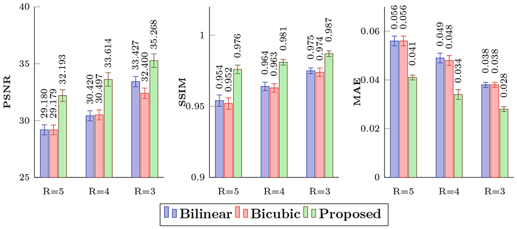
Quantitative comparison using PSNR, SSIM, and MAE.

Table 1.

Quantitative comparison of SH coefficients.

R	Bilinear	Bicubic	Proposed
3	0.128 ± 0.003	0.132 ± 0.003	0.073 ± 0.003
4	0.163 ± 0.004	0.169 ± 0.004	0.096 ± 0.005
5	0.191 ± 0.004	0.198 ± 0.004	0.101 ± 0.004

Representative reconstruction results for GFA for a fixed undersampling factor R = 4, shown in Fig. 4, indicate that the proposed method recovers the details more accurately when compared with the two interpolation methods. Figure 5 shows the representative DW images and the RMSE maps of the SH coefficients. Figure 6 shows the reconstruction results with respect to various undersampling factors. Our method consistently produces more accurate details, even for a large R.

Fig. 4.

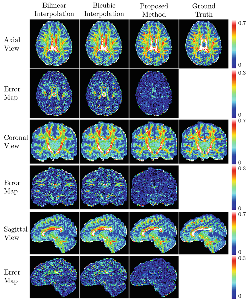
Predicted GFA maps and the corresponding error maps shown in multiple views (R = 4).

Fig. 5.

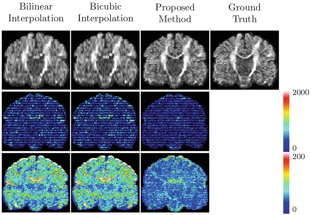
Predicted DW images (top row), the corresponding error maps (middle row), and RMSE maps of SH coefficients (bottom row) (R = 4).

Fig. 6.

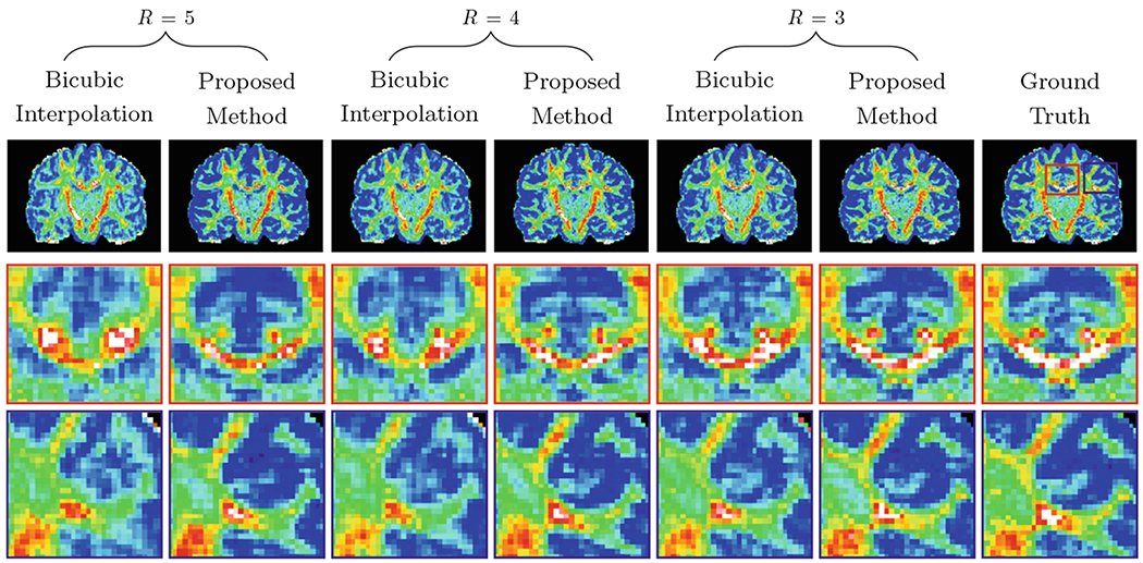
Predicted GFA maps (top row) and their close-up views (middle and bottom rows).

Figure 7 shows that our method yields fiber orientation distribution functions (ODFs) that are closer to the ground truth with less partial volume effects. We also extracted three representative tract bundles from whole brain tractography using the multi-ROI approach described in [14]. We extracted the forceps major (FMajor) using ROIs drawn in the occipital cortex and corpus callosum, and also the forceps minor (FMinor) using ROIs drawn in the prefrontal cortex and corpus callosum. For the corticospinal tract (CST), ROIs are drawn in precentral gyrus and posterior limb of the internal capsule. Figure 8 shows that our method yields richer fiber tracts that better resemble the ground truth.

Fig. 7.

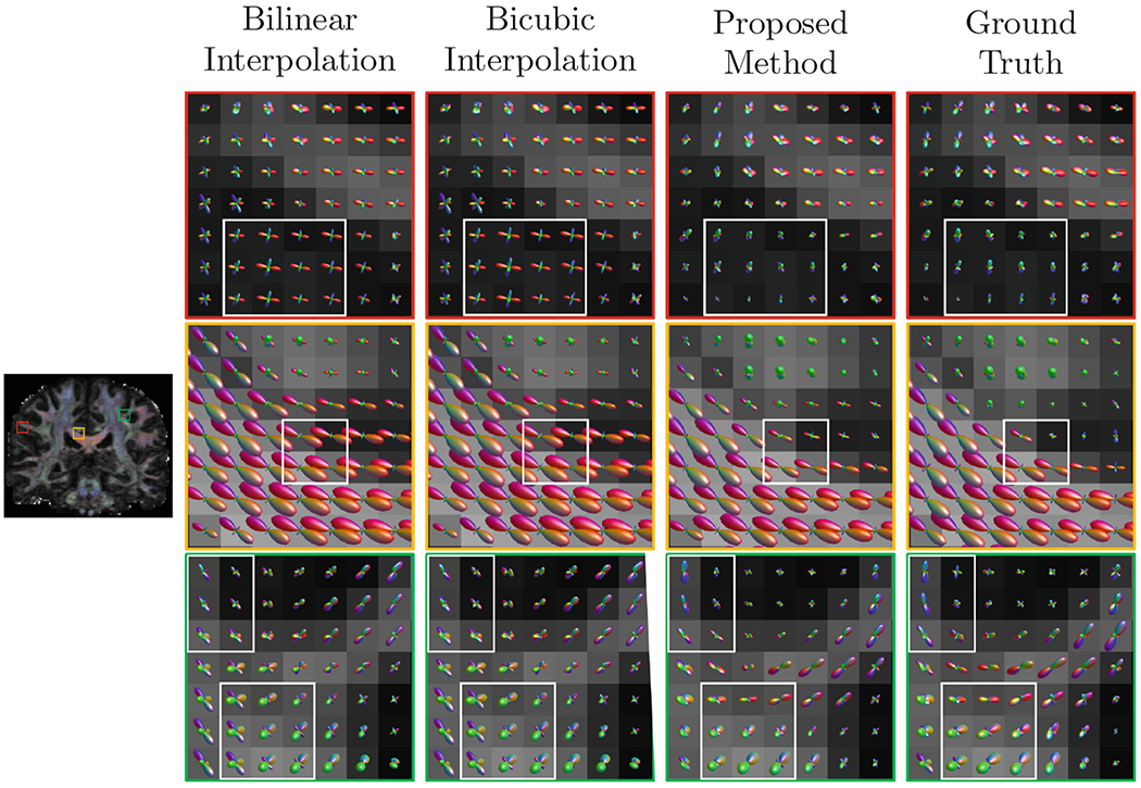
Representative fiber ODFs.

Fig. 8.

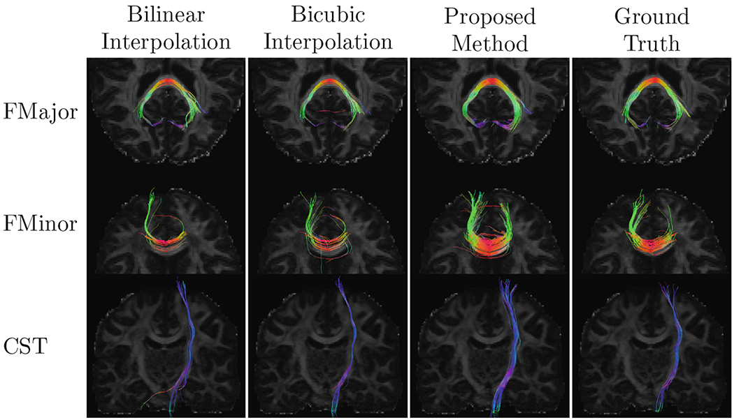
Representative tractography results.

4. Conclusion

We have proposed to employ slice-undersampling for acceleration of dMRI. Each DW image is undersampled with a different slice offset and the missing slices are reconstructed by exploiting neighborhood information in the spatial and angular domains. The non-linear mapping from slice-undersampled DW images to full DW images is learned using GCNN. Spatio-angular relationship is jointly considered when constructing the graph for the GCNN. The experimental results demonstrate that the proposed method outperforms two commonly used interpolation methods.

References

- 1.Albay E, Demir U, Unal G: Diffusion MRI spatial super-resolution using generative adversarial networks In: Rekik I, Unal G, Adeli E, Park SH (eds.) PRIME 2018. LNCS, vol. 11121, pp. 155–163. Springer, Cham: (2018). 10.1007/978-3-030-00320-3_19 [DOI] [Google Scholar]
- 2.Bronstein MM, Bruna J, LeCun Y, Szlam A, Vandergheynst P: Geometric deep learning: going beyond Euclidean data. IEEE Sig. Process. Mag 34(4), 18–42 (2017) [Google Scholar]
- 3.Bruna J, Zaremba W, Szlam A, LeCun Y: Spectral networks and locally connected networks on graphs. arXiv preprint arXiv:1312.6203 (2013) [Google Scholar]
- 4.Chen G, Dong B, Zhang Y, Shen D, Yap P-T: Neighborhood matching for curved domains with application to denoising in diffusion MRI In: Descoteaux M, Maier-Hein L, Franz A, Jannin P, Collins DL, Duchesne S (eds.) MICCAI 2017. LNCS, vol. 10433, pp. 629–637. Springer, Cham: (2017). 10.1007/978-3-319-66182-7_72 [DOI] [PMC free article] [PubMed] [Google Scholar]
- 5.Defferrard M, Bresson X, Vandergheynst P: Convolutional neural networks on graphs with fast localized spectral filtering. In: Advances in Neural Information Processing Systems (NIPS), pp. 3844–3852 (2016) [Google Scholar]
- 6.Dhillon IS, Guan Y, Kulis B: Weighted graph cuts without eigenvectors a multilevel approach. IEEE Trans. Pattern Anal. Mach. Intell 29(11), 1944–1957 (2007) [DOI] [PubMed] [Google Scholar]
- 7.Goodfellow I, et al. : Generative adversarial nets. In: Advances in Neural Information Processing Systems (NIPS), pp. 2672–2680 (2014) [Google Scholar]
- 8.Greenspan H, Oz G, Kiryati N, Peled S: MRI inter-slice reconstruction using super-resolution. Magn. Reson. Imaging 20(5), 437–446 (2002) [DOI] [PubMed] [Google Scholar]
- 9.Hammond DK, Vandergheynst P, Gribonval R: Wavelets on graphs via spectral graph theory. Appl. Comput. Harmon. Anal 30(2), 129–150 (2011) [Google Scholar]
- 10.He K, Zhang X, Ren S, Sun J: Deep residual learning for image recognition. In: Computer vision and pattern recognition (CVPR), pp. 770–778 (2016) [Google Scholar]
- 11.Henaff M, Bruna J, LeCun Y: Deep convolutional networks on graph-structured data. arXiv preprint arXiv:1506.05163 (2015) [Google Scholar]
- 12.Isola P, Zhu JY, Zhou T, Efros AA: Image-to-image translation with conditional adversarial networks. In: Computer Vision and Pattern Recognition (CVPR), pp. 1125–1134 (2017) [Google Scholar]
- 13.Long J, Shelhamer E, Darrell T: Fully convolutional networks for semantic segmentation. In: Computer Vision and Pattern Recognition (CVPR), pp. 3431–3440 (2015) [DOI] [PubMed] [Google Scholar]
- 14.Mori S, Crain BJ, Chacko VP, Van Zijl PC: Three-dimensional tracking of axonal projections in the brain by magnetic resonance imaging. Ann. Neurol 45(2), 265–269 (1999) [DOI] [PubMed] [Google Scholar]
- 15.Nie D, Wang L, Adeli E, Lao C, Lin W, Shen D: 3-D fully convolutional networks for multimodal isointense infant brain image segmentation. IEEE Trans. Cybern 49(3), 1123–1136 (2019) [DOI] [PMC free article] [PubMed] [Google Scholar]
- 16.Ning L, et al. : Sparse reconstruction challenge for diffusion MRI: validation on a physical phantom to determine which acquisition scheme and analysis method to use? Med. Image Anal 26(1), 316–331 (2015) [DOI] [PMC free article] [PubMed] [Google Scholar]
- 17.Ning L, et al. : A joint compressed-sensing and super-resolution approach for very high-resolution diffusion imaging. NeuroImage 125, 386–400 (2016) [DOI] [PMC free article] [PubMed] [Google Scholar]
- 18.Peled S, Yeshurun Y: Superresolution in MRI: application to human white matter fiber tract visualization by diffusion tensor imaging. Magn. Reson. Med 45(1), 29–35 (2001) [DOI] [PubMed] [Google Scholar]
- 19.Ronneberger O, Fischer P, Brox T: U-Net: convolutional networks for biomedical image segmentation In: Navab N, Hornegger J, Wells WM, Frangi AF (eds.) MICCAI 2015. LNCS, vol. 9351, pp. 234–241. Springer, Cham: (2015). 10.1007/978-3-319-24574-4_28 [DOI] [Google Scholar]
- 20.Scherrer B, Afacan O, Taquet M, Prabhu SP, Gholipour A, Warfield SK: Accelerated high spatial resolution diffusion-weighted imaging In: Ourselin S, Alexander DC, Westin C-F, Cardoso MJ (eds.) IPMI 2015. LNCS, vol. 9123, pp. 69–81. Springer, Cham: (2015). 10.1007/978-3-319-19992-4_6 [DOI] [PMC free article] [PubMed] [Google Scholar]
- 21.Scherrer B, Gholipour A, Warfield SK: Super-resolution reconstruction to increase the spatial resolution of diffusion weighted images from orthogonal anisotropic acquisitions. Med. Image Anal 16(7), 1465–1476 (2012) [DOI] [PMC free article] [PubMed] [Google Scholar]
- 22.Shi F, Cheng J, Wang L, Yap P-T, Shen D: Super-resolution reconstruction of diffusion-weighted images using 4D low-rank and total variation In: Fuster A, Ghosh A, Kaden E, Rathi Y, Reisert M (eds.) Computational Diffusion MRI. MV, pp. 15–25. Springer, Cham: (2016). 10.1007/978-3-319-28588-7_2 [DOI] [PMC free article] [PubMed] [Google Scholar]
- 23.Shi W, et al. : Real-time single image and video super-resolution using an efficient sub-pixel convolutional neural network. In: Computer Vision and Pattern Recognition (CVPR), pp. 1874–1883 (2016) [Google Scholar]
- 24.Sotiropoulos SN, et al. : Advances in diffusion MRI acquisition and processing in the human connectome project. NeuroImage 80, 125–143 (2013) [DOI] [PMC free article] [PubMed] [Google Scholar]
- 25.Van Steenkiste G, et al. : Super-resolution reconstruction of diffusion parameters from diffusion-weighted images with different slice orientations. Magn. Reson. Med 75(1), 181–195 (2016) [DOI] [PubMed] [Google Scholar]
- 26.Yap PT, Zhang Y, Shen D: Multi-tissue decomposition of diffusion MRI signals via ℓ0 sparse-group estimation. IEEE Trans. Image Process 25(9), 4340–4353 (2016) [DOI] [PMC free article] [PubMed] [Google Scholar]
- 27.Ye C, Zhuo J, Gullapalli RP, Prince JL: Estimation of fiber orientations using neighborhood information. Med. Image Anal 32, 243–256 (2016) [DOI] [PMC free article] [PubMed] [Google Scholar]