Absolute quantitation of microbes using 16S rRNA gene metabarcoding: A rapid normalization of relative abundances by quantitative PCR targeting a 16S rRNA gene spike‐in standard

Abstract

Metabarcoding of the 16S rRNA gene is commonly used to characterize microbial communities, by estimating the relative abundance of microbes. Here, we present a method to retrieve the concentrations of the 16S rRNA gene per gram of any environmental sample using a synthetic standard in minuscule amounts (100 ppm to 1% of the 16S rRNA sequences) that is added to the sample before DNA extraction and quantified by two quantitative polymerase chain reaction (qPCR) reactions. This allows normalizing by the initial microbial density, taking into account the DNA recovery yield. We quantified the internal standard and the total load of 16S rRNA genes by qPCR. The qPCR for the latter uses the exact same primers as those used for Illumina sequencing of the V3‐V4 hypervariable regions of the 16S rRNA gene to increase accuracy. We are able to calculate the absolute concentration of the species per gram of sample, taking into account the DNA recovery yield. This is crucial for an accurate estimate as the yield varied between 40% and 84%. This method avoids sacrificing a high proportion of the sequencing effort to quantify the internal standard. If sacrificing a part of the sequencing effort to the internal standard is acceptable, we however recommend that the internal standard accounts for 30% of the environmental 16S rRNA genes to avoid the PCR bias associated with rare phylotypes. The method proposed here was tested on a feces sample but can be applied more broadly on any environmental sample. This method offers a real improvement of metabarcoding of microbial communities since it makes the method quantitative with limited efforts.

Here, we present a spike‐and‐recovery method to get quantitative estimates from 16S rRNA surveys. The method relies on adding an artificial strand of DNA to the lysis buffer before the DNA extraction and measuring its recovery either by direct sequencing or by quantitative polymerase chain reaction (qPCR). The low detection limit achieved by qPCR allows to add minute amounts of the internal standard so that the sequencing effort is focused on the unknown sequences.

1. INTRODUCTION

Metabarcoding based on the ribosomal RNA operon is a common tool in microbial ecology to measure the relative abundance of specific microbes. The typical pipeline to study the 16S rRNA genes characterizing a microbial community involves extracting microbial DNA from the sample and sequencing. A variety of pipelines is available to then get a relative abundance table of operational taxonomic units (OTUs; Sun et al., 2011). While the choice of the pipeline can certainly affect the results, the training set (Werner et al., 2012) and the method of normalization (Kumar et al., 2018) also have a major impact even though it is seldom discussed. The most common normalization procedure consists in dividing by the total number of reads in order to obtain the proportion of each OTU. This method creates a link between the OTUs (as the sum is constant) and converts each abundance to a ratio providing relative abundances, thereby introducing ambiguity to interpret an increase in relative abundance of an OTU as an enrichment of this OTU. Therefore, there is a need to measure the absolute quantity of OTUs per weight of sample, which seems to be key for many processes such as: uptake of bacterial cells by the host (Lee et al., 2015), production of bacterial metabolites linked to obesity (Rastelli, Knauf, & Cani, 2018), or microbial production of secondary bile acids altering the liver metabolism (Ipharraguerre, Pastor, Gavaldà‐Navarro, Villarroya, & Mereu, 2018).

Measuring the absolute quantity of the OTUs is more powerful than settling for their ratio, especially in cases where the initial microbial density varies substantially. For example, the relative abundance of OTU X might be identical in sample A and sample B while its absolute concentration could be three times lower if sample B has a third of the overall bacterial density of sample A (Props et al., 2017). This is biologically relevant because 10‐fold variation in the microbial load was observed in human fecal samples and linked to the enterotype (Vandeputte et al., 2017). Furthermore, inferring the interaction networks suffers from a compositionality effect when using relative abundance data rather than absolute abundance data (Jackson, 1997; Vandeputte et al., 2017). Looking at the ratios between species or at the variations of the species abundance curve can circumvent the bias of the relative composition data for time series sampled frequently (Morton et al., 2019), but it is less precise than absolute quantification.

Recent years have seen an effort in measuring absolute quantity of microbes rather than settling for their proportion (Table 1). For example, quantitative polymerase chain reaction (qPCR) was used to evaluate the absolute abundance of fungi from their relative abundances measured by 454 sequencing (Dannemiller, Lang‐Yona, Yamamoto, Rudich, & Peccia, 2014). Flow cytometry has been used to estimate the absolute concentration of their OTUs and avoid spurious relationships due to proportions in environmental (Props et al., 2017) or fecal (Vandeputte et al., 2017) samples. The latter study showed that qPCR (without any internal standard to measure DNA recovery yield) was not as efficient as flow cytometry. Another solution to take into account the microbial density is to spike the samples with a known number of cells. For example, Stämmler et al spiked mice fecal samples with a mixture of bacteria that do not exist in the gut microbiome under physiological conditions in order to quantify the OTU (Stämmler et al., 2016). More recently, Piwosz and colleagues added 7.5 × 10⁷ Escherichia coli cells per sample in order to reconstruct the absolute abundance of the other OTUs present in the sample (Piwosz et al., 2018).

Table 1.

Comparison of available methods to evaluate the absolute concentration of microbes in environmental samples

Addition of	Detection method	Measures	Goal of normalization	Limitation	Reference
—	16S sequencing	Relative abundance of reads within each sample		No quantification between samples	Verschuren et al. (2018)
—	Flow cytometry 16S sequencing	Relative abundance of OTU Cell number per mg	Initial density	The flow cytometer requires fresh samples Potential bias if cells cannot be extracted/amplified	Vandeputte et al. (2017)
Microbial cells to the sample	6S sequencing	OTU abundance relative to E.coli	Initial density/extraction efficiency	The species have to be absent from the samples	Piwosz et al. (2018), Stammler et al. (2018)
Genomic DNA	Shotgun sequencing		Performance of metagenomics workflows	The species have to be absent from the samples	Venkataraman et al. (2018)
Synthetic DNA internal standard	16S sequencing of the V4 region	Relative abundance of reads	Initial density/extraction efficiency to obtain number of OTU per mg (optionally converted to cells per mg via database)	20%–80% devoted to measure the DNA internal standard Dose of internal standard difficult to calibrate Can only be used with 515F/806R Assumes 100% lysis in the first step of the DNA extraction	Tkacz et al. (2018)
	Sequencing qPCR	Relative abundance of reads 16S rRNA copies per mg	Initial density/extraction efficiency to obtain number of OTU per mg	Assumes 100% lysis in the first step of the DNA extraction	This study

Abbreviations: OUT, operational taxonomic unit; qPCR, quantitative PCR.

Some authors use DNA spike‐in rather than whole cells because DNA quantitation is easier, more accurate and reproducible. Venkataraman and colleagues demonstrated the usefulness of such a standard in studies based on shotgun sequencing (Venkataraman et al., 2018), but it still required the prior knowledge of the DNA that might be present in the samples.

In order to create a spike‐in standard that does not require prior knowledge of the species already present in the samples, Tkacz et al created a synthetic standard for metabarcoding that cannot be found in any known living cells (Tkacz, Hortala, & Poole, 2018), which allowed them to quantify the absolute abundance of prokaryotic 16S, eukaryotic 18S, and fungal ITS in soil samples with three separate sequencing reactions. However, this strategy still requires an accurate estimation of the bacterial density in the sample because the DNA internal standard has to be added at the amount matching 20%–80% of the 16S rRNA genes. It should be noted that this also means that a very large part of the sequencing effort is dedicated to the standard. Furthermore, this standard can only be used with the primer set 515F/806R.

Here, we describe a synthetic DNA internal standard than can be quantified by qPCR in order to take the DNA recovery yield into account (Figure A1). This standard can also be quantified by direct sequencing targeting either the V3‐V4 or the V4‐V5 regions of the 16S rRNA gene with any primer flanking the V3 and/or the V4 and/or the V5 hypervariable regions of the 16S rRNA gene. We also used the sequencing primers to estimate the bacterial load so that we optimally determine the absolute quantitation of each OTU based on sequencing and qPCR. The method proposed here was tested on a fecal sample but can be applied virtually on any environmental sample.

2. MATERIAL AND METHODS

2.1. Design and production of the synthetic spike used as DNA internal standard

The production of the DNA internal standard was performed according to the following steps (Figure A2):

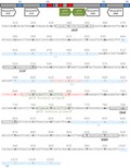
Step 1: Amplify the relevant region of the 733 bp—long DNA internal standard. These 733 bp are exactly the 733 bp from E. coli str. K‐12 substr. MG1655 NC_000913.3:4035531‐4037072, except that 45 base pairs between the positions 610 and 700 (in the region 4) were modified with identifiable patterns of 17, 16, and 12 bp (Figure 1). These 45 bases were chosen to avoid the secondary structures of the 16S rRNA gene and enable an easy quantification of the DNA internal standard either by sequencing or by qPCR. In our case, the synthetic sequence ordered from GeneArt (Thermo Fisher) was delivered in the plasmid pMK (Thermo Fisher) and the production of the synthetic sequence was performed with the 343F/784R primer pair with the Illumina miseq adapters for the product added in the samples (i.e., 5′‐CTTTCCCTACACGACGCTCTTCCGATCTTACGGRAGGCAGCAG and 5′‐GGAGTTCAGACGTGTGCTCTTCCGATCTTACCAGGGTATCTAATCCT), and with the 343F/908R primer pair with the Illumina miseq adapters (i.e., 5′‐GGAGTTCAGACGTGTGCTCTTCCGATCTCCCCGYCAATTCMTTTRAGT) in order to generate standard curves that can be used with 343F/784R or 515F/908R.

Figure 1.

Schematic representation (TOP) and actual sequence of the 732bp‐DNA internal standard based on E. coli K12 MG1655 (BOTTOM). The bases differing between E. coli and the synthetic DNA internal standard are indicated in red. The primer pair E targets the DNA internal standard that is spiked in the samples. The other primers with the Illumina miseq adapters are targeting all 16S rRNA genes (including the internal standard). The numbering corresponds to the bases in bold. The hypervariable regions of the 16SrRNA gene are in blue. Binding sites of qPCR primers are in green. Binding sites of primers used in this study are boxed

Step 2: Purify the amplicon using the Illustra microspin G‐50 kit (GE Healthcare) by centrifugating the PCR product at 450 g for 5 min after a preparation spin of 450 g for 5 min (Figure A2).

Step 3: Quantify the PCR product by Qubit 2.0 Fluorometer (Invitrogen), adjust the concentration to 20 ng/µl, and convert to a copy number with the help of the size of the amplicon (equivalent to 2.8 × 10⁹ copies/µl when the 343F/908R primers are used).

2.2. DNA extraction, 16S sequencing, data storage, and production of the OTU table

Step 4: Weigh each sample (our samples weighed between 9.3 and 55 mg).

Step 5: Add the DNA internal standard to the lysis buffer at the appropriate amount and extract the microbial DNA from the samples using this lysis buffer. For example, for 20 samples we added 20 × 10⁸ copies of DNA internal standard to the 24 × 400 µl of lysis buffer that we needed for the extraction using the Quick‐DNA™ Fecal or Soil Microbe Miniprep Kit™ (Zymo Research) according to the manufacturer's instruction. A 15‐min bead‐beating step at 30 Hz was applied using a Retsch MM400 Mixer Mill. The elution volume was 100 µl.

Step 6: Amplify the variable regions of the 16S rRNA gene with compatible primers and sequence with the Illumina chemistry. Here, we used the 343F and 784R primers and the pipeline described previously (Verschuren et al., 2018). Briefly, the V3V4 region was amplified from purified genomic DNA (gDNA) with the primers F343 and R784 using 30 amplification cycles with an annealing temperature of 65° to produce a 510 bp amplicon, although the exact length varies depending on the organisms. Because MiSeq enables paired 250‐bp reads, the ends of each read are overlapped and can be stitched together to generate extremely high‐quality, full‐length reads of the entire V3 and V4 region in a single run. Single multiplexing was performed using home made 6 bp index, which was added to R784 during a second PCR with 12 cycles using forward primer (AATGATACGGCGACCACCGAGATCTACACTCTTTCCCTACACGAC) and reverse primer (CAAGCAGAAGACGGCATACGAGAT‐index‐GTGACTGGAGTTCAGACGTGT). The resulting PCR products were purified and loaded onto the Illumina MiSeq cartridge according to the manufacturer instructions. The quality of the run was checked internally using PhiX, and then each pair‐end sequences were assigned to its sample with the help of the previously integrated index. Each pair‐end sequences were assembled using Flash software (Magoc & Salzberg, 2011) using at least a 10 bp‐overlap between the forward and reverse sequences, allowing 10% of mismatch. All the sequences are publically available on NCBI under the BioProject PRJNA531076. They were processed with the DADA2 pipeline (Callahan et al., 2016) with the following parameters: trim 17 bp from each fragment to remove the primers, filter out the sequences below 390 bp after merging R1 and R2 or sequences with undetermined bases, remove the chimera using the consensus method.

Step 7 (only if the abundance of DNA internal standard is high enough for direct quantification from the sequences): The identification of our DNA internal standard in the sequencing data was performed by finding the following pattern in the sequence: "ATCGATCG.*.ACGTACGTACGT.*.CGATTGAAAT."

2.3. qPCR on the DNA internal standard

Step 8a: Create tubes containing 10–10⁸ copies of the 343F/908R amplicon of DNA internal standard (see above; Figure A2).

Step 8b: Create tubes containing 2.5 μl of 100‐fold diluted DNA extracted from a sample spiked with 10⁸ copies of DNA internal standard per tube.

Step8c: Create a tube containing 2.5 μl of 100‐fold diluted DNA extracted from a unspiked sample to check that the sample does not contain any fragment amplifiable with the primer pair E.

Step 9: Add 0.1 μl of forward and reverse primers E 5′‐CAGATGTGAAATCATCGATCG/5′‐CCGATTTCAATCGTACACCTG, 5 μl PowerUp SYBR Green Master Mix (Thermo Fisher Scientific) and 2.3 μl sterile nuclease‐free water to obtain PCR mixtures of 10 µl. Note that the forward primer E was designed to overlap two out of three tags of the DNA internal standard (Figure 1).

Step 10: Run 40 cycles of a two step program (95°C for 30 s and 60°C for 3 min) to allow complete elongation of the long amplicons on the QuantStudio 6 Flex system with 384‐well plates. Note that the 3‐min elongation is useful to run the qPCR of the total 16S on the same plate (see below). Check the lack of amplification in the unspiked sample and convert the cycle threshold into a number of copies with the help of the standard curve.

2.4. qPCR to quantify the 16S rRNA genes

Step 11: Create tubes containing 10–10⁸ copies of the 343F/908R amplicon of DNA internal standard after purification and quantification (see above). Note that the DNA internal standard is also used to calibrate the qPCR targeting the 16S rRNA gene with the 343F/784R primers because the sequence of the DNA internal standard is identical to the E. coli sequence at the binding sites of 343F and 784R.

Step 12: Add 0.1 μl of 343F/784R primers to the PCR assay mixtures consisting of 5 μl PowerUp SYBR Green Master Mix (Thermo Fisher Scientific), 2.3 μl sterile nuclease‐free water, and 2.5 μl template DNA diluted 100‐fold. Note that amplifying with the 515F/806R primers is also possible.

Step 13: Run 40 cycles of a two step program (95°C for 30 s and 60°C for 3 min) to allow complete elongation of the long amplicons on the QuantStudio 6 Flex system with 384‐well plates. Note that the 3‐min elongation is useful because the amplicon is longer than those typically used in qPCR (441 bp instead of 150 bp). Convert the cycle threshold into a number of copies with the help of the standard curve.

2.5. Standardization method

The standardization had to be applied to any OTU in order to obtain the amount of each OTU per weight of sample. It uses the percentage of the relevant OTU in the sequencing data, the quantification of the DNA internal standard by qPCR and the quantification of the total 16S by qPCR.

Step 14: Quantify the extraction yield (E _extraction) by dividing the number of copies of DNA internal standard that was measured in Step 10 ($Q_{\text{Standard}}^{\text{measured}}$ in copies/µl) by the number of copies that were added in Step 5 ($Q_{\text{Standard}}^{\text{added}}$). Typically, this step requires to take into account the volume in which the DNA was eluted (here 100, see Step 5) and the dilution factor used before the qPCR (here 100, see Step 8).

$$E_{\text{extraction}}=\frac{Q_{\text{Std}}^{\text{retrieved}}}{Q_{\text{Std}}^{\text{added}}}=\frac{\text{Std}\_\text{measured}\_\text{qPCR}(\text{copies})\times 100\times 100}{{10}^8}$$

Step 15: Multiply this extraction yield by the number of 16S copies per the weight (W) of the fecal samples used for the extraction (qPCR on a diluted sample) and the ratio of each OTU in the sequencing data. For example, the normalized abundance of the first OTU in the first sample is as follows:

$$\begin{array}{cc}& \text{OTU}\_1(\text{copies per weight})\hfill \\ \hfill & =\frac{\frac{\text{Counts}\_\text{OTU}\_1\_\text{in}\_\text{sample}\_1}{\text{total}\_\text{number}\_\text{reads}\_\text{in}\_\text{sample}\_1}\times Q_{\text{total}16\mathrm{S}}^{\text{Step}13}(\text{copies})\times E_{\text{extraction}}}{\text{Sample}\_\text{Weight}}\hfill \end{array}$$

where $Q_{\text{total}16S}^{\text{Step}13}$ is the number of copies of 16S rRNA genes measured in Step 13.

2.6. Experiment 1: Testing the range of concentrations of the DNA internal standard

In order to check the linearity of the quantification with various ratios of biomass over DNA internal standard, we tested various amounts of DNA internal standard in Step 5, namely 2.8 10⁶, 2.8 10⁷, 1.4 × 10⁸, and 2.8 × 10⁸ copies of DNA internal standard to extract 38, 55, 38, and 43 mg of feces originating from a 99‐day‐old sow (hence, aiming for 0.05%–4% of the abundance of 16S rRNA genes).

2.7. Experiment 2: Mimicking the abundance increase of an OTU in a feces sample

In order to mimic the increase of abundance of an OTU in an otherwise stable community, we added E. coli cells to fecal samples from a 99‐day‐old sow. The exact weight of each sample was recorded with a Mettler AE200 scale (Mettler Toledo) with 0.1 mg precision, and they varied between 9.3 and 16.1 mg. The E. coli strain was previously isolated in the laboratory and grown overnight in 24ml of Luria‐Bertani (LB) medium at 30°C. The cells were then centrifuged at 8,000 g during 5 min at 20°C in order to reduce the volume to 450 µl of suspension. We added in triplicates 0, 1, 5, 10, and 100 µl of the E. coli suspension at 10⁷ cells/µl to approximately 10 mg of fecal sample (the exact weight varied between 9.3 and 16 mg) to the 15 tubes labeled in ascending order (i.e., a range between 0 and 8.6 × 10⁷ cells/mg). The exact cell density of 1.1 10⁷ ± 2.7 × 10⁶ cell/µl was determined by plating a serial dilution on LB plates in triplicates. The DNA internal standard was added at 2.7 × 10⁷ copies per tube by adding it to the 400 µl of BashingBead lysis buffer used for the DNA extraction (hence approx 1% of the concentration of total 16S copies based on the assumption that fecal samples have 10¹⁰ bacterial cell/mg). The DNA recovery was measured in the 15 tubes. One of each triplicate was sequenced (hence five tubes), and the standard deviation was approximated by the binomial law.

3. RESULTS

The internal standard is an artificial DNA sequence that contains specific ATCG pattern that sets it apart from every sequence of 16S rRNA gene entered in Genbank. The DNA sequence is added to the sample before the DNA extraction so its recovery can quantify the extraction yield. We can then calculate the absolute numbers of 16S rRNA genes in the sample after lysis from the qPCR measurement targeting the 16S rRNA genes and this extraction yield. Here, we first verify the linearity of the signal across the range of detection. Second, an experiment using E. coli cells was performed to check for the accuracy of the method.

3.1. Wide acceptable range for the ratio between internal primer and total 16S rRNA gene

The efficiency of the primers pair E detecting the DNA internal standard across the serial dilutions was 90% (Figure A3), allowing an accurate quantification of the internal standard. The quantification was linear from 10² to 10⁸ copies/µl (R ² = .99; Figure A3), which allows a very wide range of detection of 6 log. The efficiency of the primers detecting the load of 16S rRNA gene by qPCR with the 343F/784R primer pair was satisfying (68.7%; R ² = .998; Figure A4). Both primers had the same useable range, that is, from 10² to 10⁸ copies per PCR reaction. Unsurprisingly, the quantification of the internal standard was linear in the four samples in which the internal standard represented between 0.05% and 3.8% of the total number of 16S rRNA genes (data not shown). The DNA recovery yield was 46 ± 4% for these four extractions performed on the same fecal sample. Hence, the quantification of the internal standard is accurate and independent of the biomass present in the sample.

3.2. Detection of an OTU whose abundance is increasing

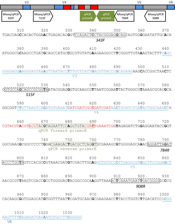
The value of an absolute quantity of microbes to understand the dynamics of the species between samples is obvious in the event of the strong increase of the abundance of an OTU while most OTUs remain stable. To mimic this situation, we added different quantities of E. coli cells to a pig fecal sample—that is, between 0 and 8 × 10⁷ per mg of feces, hence, creating a set of artificial samples in which all the OTUs but E. coli remain constant. We then demonstrate that the use of an internal standard allows us to characterize this dynamics accurately, when the ratios obtained through the classical sequencing pipeline do not. Indeed, using the qPCR measurements to correct for the DNA recovery yield (Table 1), the total microbial load increased from 43 ± 2 to 110 ± 65 × 10⁷ copies per mg. The calculated amount of E. coli 16S rRNA genes copies varied between 10⁶ copies/mg in the tube 1 and 8 × 10⁸ copies/mg in the tube 13 (Table A2), which is relatively close to the expected values as we artificially added 8 × 10⁷ E. coli cells/mg in the tube 13 and E.coli has seven copies of rRNA genes per genome. In other words, adding one E. coli cell resulted in adding 8.9 copies of 16S genes (Figure 2). Therefore, the use of the internal standard could indeed detect the increased abundance of a particular OTU amid a complex sample containing 428 OTUs that are stable over the experiment (Figure A6).

Figure 2.

Relationship between the number of E. coli cells added and the number of E. coli 16S RNA genes as calculated by the method presented in the paper. Since each E. coli cell possesses 7 copies of 16S rRNA genes, we would expect a 7 fold difference. Yet we observe a 8.9 fold difference, meaning that each E. coli cell has 8.9 copies of 16S rRNA genes, which is likely due to residual growth of the cells. The error bars might be smaller than the symbol

3.3. Detection of the internal standard in the sequencing data

The tags of the internal standard can be used to identify the internal standard in the OTU abundance table. When using a simple proportionality method on our data (between four and nine counts out of 10,808 sequences), we obtain 1.9 higher estimates than with the qPCR (data not shown).

3.4. Measure of the gDNA recovery yield as a by‐product of internal standard addition

The qPCR method described quantifies the gDNA recovery for each sample. In the present study, the gDNA recovery across the 15 samples of experiment 1 and four samples from experiment 2 varied between 40% and 84% (60 ± 12%), which illustrates the need of an internal standard (Figure A5).

4. DISCUSSION

4.1. Usefulness of a wide acceptable range for the ratio between internal primer and total 16S rRNA gene

In this study, we propose a method to generate quantitative abundance data from microbial surveys by adding an internal standard before the DNA extraction. We also propose a qPCR‐based method as an alternative to the direct measure of this internal standard in the next generation sequencing (NGS) data. In a nutshell, the qPCR with the primer pair E quantifies the internal standard and the qPCR with the 343F/784R primers quantifies the total amount of 16S rRNA genes (the 343F/784R primers also detect the internal standard, which is a slightly modified sequence of the E. coli 16S RNA gene). Detecting the internal standard using qPCR instead of using direct counting of the sequence of the internal standard in the NGS data allows us to add minute amounts of the internal standard, which avoids sacrificing 20%–80% of the sequencing effort to the internal standard as in the method using a synthetic standard developed by Tkacz et al (Tkacz et al., 2018). Our qPCR‐based method avoids the underestimation of rare sequences by sequencing (Gonzalez, Portillo, Belda‐Ferre, & Mira, 2012). Indeed, targets below 1% are underestimated by PCR when several targets are present. Luckily, targets representing 30% of the sample are well estimated by a sequencing depth of 10⁴ sequences per sample (Gonzalez et al., 2012). Interestingly, when using a simple proportionality method on our data (between four and nine counts out of 10,808 sequences), we obtain 10‐fold higher estimates than with the qPCR, probably because the standard counts are underestimated as every other target around 1% of relative abundance. It should be noted that the underestimation of rare OTUs by PCR does not apply to the detection by qPCR which specifically targets the internal standard (hence only one target is present). In this context, adding minuscule amounts of internal standard instead of 20%–80% also avoids potential calculation mistakes that would lead to an overload of internal standard.

4.2. Usefulness of measuring of the gDNA recovery yield for qPCR estimation of the bacterial load

Another advantage of the qPCR method described here is that we were able to quantify the gDNA recovery for each sample with a 5% precision (Table A4). In the present study, the gDNA recovery varied between 46% and 84%, which is consistent with the recovery of 37% reported previously for bead‐beating methods (Vishnivetskaya et al., 2014). It is partly due to the incomplete recovery of supernatant during the DNA extraction procedure. The variability of the extraction is also observable in a study comparing technical replicates to biological replicates (Dannemiller et al., 2014). Such a variability hampers the use of qPCR without internal standard, and a twofold difference in the DNA recovery yield cannot be ignored. Indeed, Vandeputte reports a biologically relevant threefold differences in the bacterial density between patients with Crohn's disease and healthy controls (Vandeputte et al., 2017).

The internal standard should be added before the DNA extraction to get absolute quantitation. The variability of the gDNA recovery rate (and hence the variability of the DNA extraction efficiency) could partly explain the inaccuracy of microbial density estimation by qPCR when it is not combined with an internal standard correcting for the extraction efficiency (Dannemiller et al., 2014; Vandeputte et al., 2017). As a matter of comparison, Hardwick and colleagues created a set of 86 spike‐in standards for shotgun metagenomics (Hardwick et al., 2018): The 86 synthetic standards were added after the DNA extraction step, which allowed to evaluate only the sequencing biases but neither the initial abundance nor the gDNA recovery yield. Adding the internal standard prior the DNA extraction and judging the extraction efficiency is crucial. Since we added synthetic DNA, we actually measured gDNA recovery yields rather than DNA extraction efficiency, which would be the combination of efficiency of lysing cells and the gDNA recovery yield. It should be noted that bead‐beating usually destroys the cells efficiently (de Bruin & Birnboim, 2016) and protocols based on bead‐beating are recommended (Yuan, Cohen, Ravel, Abdo, & Forney, 2012). The synthetic DNA was added to the lysing buffer in order to avoid rapid degradation in the extracellular environment.

4.3. Comparison with other methods measuring absolute bacterial quantities

Several methods were proposed to design a internal standard using DNA or cells (Table 1). Some recent studies recommend using flow cytometry to evaluate the total bacterial load (Props et al., 2017; Vandeputte et al., 2017). Notwithstanding the relative difficulty of accessing a high‐quality flow cytometer able to detect bacterial cells in a timely manner, this method relies on the dissociation of the bacterial biomass into single cells by diluting, vortexing, and filtering the sample immediately after collection. This is not a trivial step for samples in which bacteria are attached together or to a substrate and the exact dissociation protocol used before flow cytometry could introduce a twofold factor (Falcioni et al., 2006), needing an inter‐laboratory calibration procedure for accurate comparison of results. For valuable or hard to recover samples, the amount of material may be limited and does not allow using material for both flow cytometry and DNA extraction. As discussed above however, the qPCR requires adding an internal standard before the DNA extraction to be accurate. In our opinion, qPCR is the unsurpassed way to normalize the sequencing data because it uses the same methodological workflow, from DNA extraction to exact same primers as the sequencing reaction. In other words, a bacterial species that cannot be amplified (because its cells are resistant to the DNA extraction protocol or its fragment is not amplified by the primers used) will not impact the calculations on the abundances observed in the sequencing data corrected with qPCR data. For species from which extracting DNA through bead‐beating is difficult, our method informs that at least X copies/mg of sample were present.

Several authors have proposed to add cells as internal standards before the DNA extraction, but we believe that adding a synthetic DNA offers more control than adding cells, whose exact number of 16S rRNA genes per cell is difficult to control. Indeed, growing E. coli cells can harbor up to 38 copies per cell, instead of the seven copies per genome due to multiple replication forks (Bremer & Dennis, 2008). Adding starved cells is more accurate (Figures A7 and A8; Table A3) but it should also be noted that databases associating genera and a 16S rRNA gene copy number are based on genome sequencing rather than actual measurements of growing cells. Therefore, any database would associate seven copies per E. coli cell (Vandamme & Coenye, 2003) even if that number might not hold in growing E. coli cells in a real‐life sample (Bremer & Dennis, 2008). This means that any estimation of a bacterial population based on 16S rRNA genes is still subject to a bias if the population is growing. For example, our E.coli population had 9.5 ± 1.5 copies/cell, which illustrates the challenge of methods based on cells rather than synthetic DNA.

Our design of the DNA internal standard includes several key features representing an improvement over the synthetic standard developed by Tkacz et al (Tkacz et al., 2018). The first improvement is the ability to add minuscule amounts of our DNA internal standard and still detect it by qPCR, which keeps the sequencing effort focused on unknown microbes as mentioned above. Secondly, the wide measurement range makes it possible to add the same amount of DNA internal standard to every sample whatever the number of cells. One easy way to use our DNA internal standard is by adding it to the lysis buffer, which makes it a very simple protocol modification. Thirdly, our standard is able to cope with V3‐V4 or V4‐V5 regions of the 16S rRNA gene, which gives better resolution than just the V4 region of Tkacz et al (Tkacz et al., 2018). Our DNA internal standard is compatible with any primer flanking these regions because we simply added tags in the V4 region of the 313‐1034 fragment of the 16S rRNA gene. Therefore, in addition to the primers used in this study, the following primers are also compatible with our DNA internal standard according to the nomenclature of Baker and colleagues (Baker, Smith, & Cowan, 2003): E334F,E341F, U341F, U515, U519F, E926R, U926R, and E939R. Fourthly, the tags of the DNA internal standard minimize the potential PCR bias. This bias is avoided because the backbone sequence of the DNA internal standard is based on E. coli and the 45 modified bases avoid the know secondary structures while keeping a balanced GC content, as the GC content of the sequence could impact the proportion in the sequencing data (Aird et al., 2011).

4.4. Application range of our DNA internal standard system

Despite quantifying precisely the number of 16S rRNA gene copies in a sample, the DNA internal standard does not solve common limitations of the PCR‐based methods linked to the number of 16S rRNA gene copies per cell or to the cell‐specific difference in extraction efficiency such as spores recalcitrance (de Bruin & Birnboim, 2016). It should be noted that PCR inhibitors would impact the qPCR estimation. As such, we recommend to check the efficiency of every amplification curve and to apply individual linear regression (Ruijter et al., 2009) or add polyvinylpolypyrrolidone to remove PCR inhibitors if necessary (Fuentes & Arbeli, 2007).

In conclusion, we recommend to routinely add a DNA internal standard to any environmental sample to be sequenced before DNA extraction. The small amounts of added DNA internal standard allowed by our qPCR method (0.05% of the total 16S rRNA gene copies if qPCR is used, 20% if the DNA internal standard is estimated from the sequencing data) and the similarity with E. coli 16S rRNA ensure that this addition does not hinder the classical metabarcoding pipeline. This addition allows correcting for the initial bacterial density, thereby allowing researchers to better link their microbial data with the phenotypes for which the absolute concentration of the bacteria is critical. Furthermore, quantification using a DNA internal standard could partly compensate for the different extraction methods needed in real‐world research. This feature is essential since the methodology presented here is intended to be applicable to many complex environments such as soil, sediment, compost, biofilm, engineered environments, and gut.

CONFLICT OF INTEREST

The authors declare no conflict of interest.

AUTHOR CONTRIBUTIONS

OZ, JJG, CA, LV, and JH conceptualized the data; LC involved in data curation; OZ formally analyzed the data and involved in funding acquisition, project administration, and resources; BG, MLDA, and LV performed investigation; OZ, MLDA, and LV involved in methodology; OZ and JJG involved in supervision and wrote the original draft; BG performed validation; all authors wrote, reviewed, and edited the article.

ETHICS STATEMENT

None required.

Appendix 1.

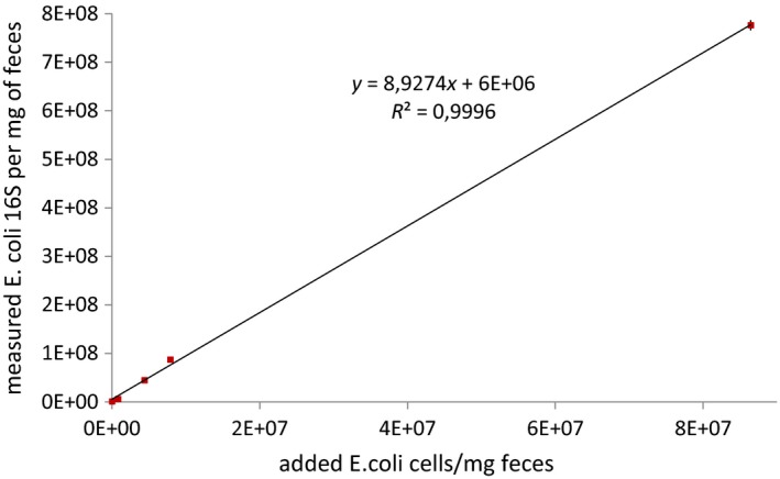
1. Comparison of the traditional pipeline to analyse 16S rRNA surveys and the use of an internal standard

Figure A1.

The principle of the method relies in adding a known amount synthetic strand of DNA before the extraction step (in the figure, 2 copies/g) in order to estimate the DNA recovery yield during the extraction. This information allows to use to quantification of the extracted DNA at the end of the extraction step to estimate the initial abundance of the suspended DNA just after lysis

The pipeline using the internal standard estimates the number of 16S rRNA copies per gram of sample, instead of simply estimating ratios. This is very useful if samples with varying densities are to be compared.

It should be noted that the ratio of internal standard vs 16S rRNA genes can be estimated either by direct counting in the sequencing data or by qPCR. The qPCR offers a wide range which avoids a difficult initial guess of the microbial density in each sample.

2. Schematic of the pipeline using the internal standard and qPCR

Figure A2.

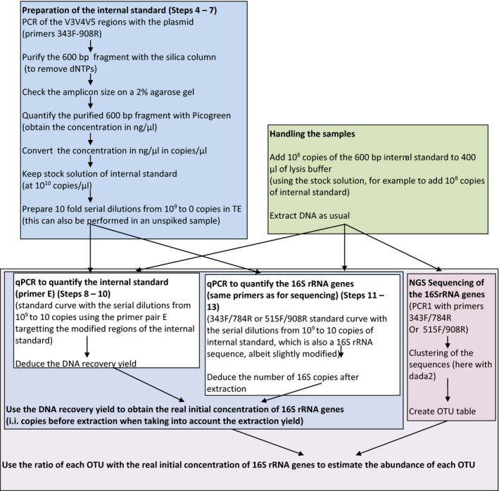
Detailed schematic of the pipeline using the internal standard estimated by quantitative PCR and NGS

It should be noted that the nub of the method relies in the estimation of the internal standard to correct for the DNA recovery yield. The quantitative PCR allows to add small amounts of the internal standard, which avoids to overshoot and hinder the sequencing data by simply sequencing too much internal standard. When using high amounts of internal standard, the qPCR is not useful as the sequencing data can be used directly.

3. Quantitative PCR of the internal standard and total 16S rRNA genes

3.1 Principle of quantitative PCR

The quantitative PCR is a PCR in which the fluorescence is measured at the end of each cycle. The fluorescence is proportional to the number of double‐stranded DNA strands. In the paragraph below we outline how this technology can be used to quantify the internal standard and the total number of 16S rRNA genes (including the internal standard). In order to estimate the initial concentration of 16S rRNA. The total number of rRNA genes is then corrected by the DNA recovery yield.

3.2 Quantification of the internal standard with primers E

Figure A3.

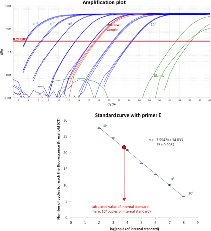
Standard curves of the quantitative PCR to measure the DNA internal standard (TOP) and the corresponding amplification curves with the serial dilutions of the internal standard (BOTTOM). The tubes from the serial dilutions that are used to calculate the primers' efficiency are in blue (here 91%). The triplicate measure on a tube from the experiment are in red. The PCR blanks are in green. The standard deviation can be smaller than the symbol

3.3 Quantification of the total 16S rRNA genes with 343F/784R

Figure A4.

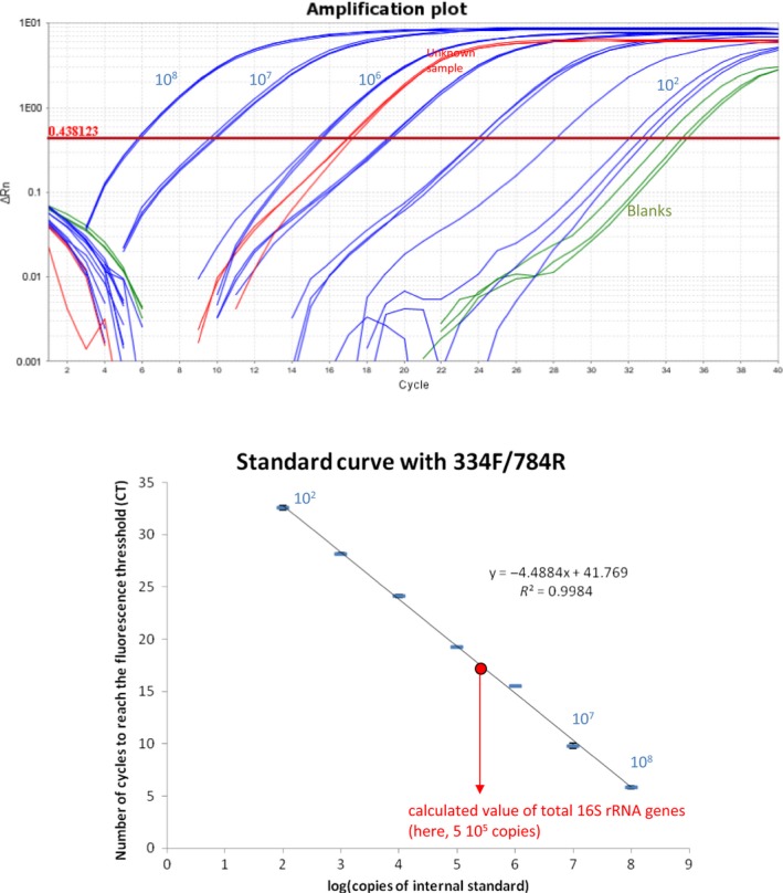
Standard curves of the quantitative PCR to measure the total 16S rRNA copies (TOP) and the corresponding amplification curves with the serial dilutions of the internal standard (which is a modified 16S sequence) (BOTTOM). The tubes from the serial dilutions that are used to calculate the primers' efficiency are in blue (here 68%). The triplicate measure on a tube from the experiment are in red. The PCR blanks are in green. The standard deviation can be smaller than the symbol

3.4 Calculation of the efficiency of the primers

The efficiency of the primers (E) was calculated using the serial dilutions containing 100 to 10⁸ copies of the internal standard with: E = 10^(−1/slope)−1.

4. Detailed data of the supplementation experiment

4.1 Complete qPCR data for the 15 samples with increasing E. coli concentrations

Table A1.

qPCR data for the 15 samples with increasing E. coli concentration

		1	2	3	4	5	6	7	8	9	10	11	12	13	14	15
Data for qPCR method	mgfeces	11.2	10.2	12.4	13.1	9.6	11.4	12.5	9.9	9.3	13.9	13	9.7	12.7	11.1	16.1
	added_std	3.E+07	3.E+07	3.E+07	3.E+07	3.E+07	3.E+07	3.E+07	3.E+07	3.E+07	3.E+07	3.E+07	3.E+07	3.E+07	3.E+07	3.E+07
	added_std_per_mg	2.E+06	3.E+06	2.E+06	2.E+06	3.E+06	2.E+06	2.E+06	3.E+06	3.E+06	2.E+06	2.E+06	3.E+06	2.E+06	3.E+06	2.E+06
	Velution	100	100	100	100	100	100	100	100	100	100	100	100	100	100	100
	dilutionfactor	100	100	100	100	100	100	100	100	100	100	100	100	100	100	100
qPCR measurements	Std_M1(copies/µlPCR)	2,082	1,880	1,886	1,762	2,443	2,048	1,834	1,914	2,044	1,706	1,729	1,873	1,357	1,232	1,469
	Std_M2(copies/µlPCR)	1,526	1,935	1,568	1,819	2,073	2,178	1,712	1,834	1,761	1,682	1,780	1,980	1,267	1,227	1,458
	Std_M3(copies/µlPCR)	1,704	1,970	2,005	1,826	2,512	2,064	1,898	1,802	1,730	1,823	1,767	1,998	1,368	1,378	1,730
	Std_in_tube (copies)	2.E+06	2.E+06	1.E+06	1.E+06	2.E+06	2.E+06	1.E+06	2.E+06	2.E+06	1.E+06	1.E+06	2.E+06	1.E+06	1.E+06	1.E+06
	DNA recovery yield	0.64	0.69	0.66	0.65	0.84	0.75	0.65	0.67	0.66	0.63	0.63	0.70	0.48	0.46	0.56
	total16S_M1(copies/µl pcr)	3.E+05	4.E+05	4.E+05	4.E+05	3.E+05	4.E+05	3.E+05	3.E+05	2.E+05	4.E+05	4.E+05	4.E+05	8.E+05	9.E+05	3.E+05
	total16S_M2(copies/µl pcr)	3.E+05	2.E+05	4.E+05	2.E+05	3.E+05	2.E+05	4.E+05	2.E+05	3.E+05	3.E+05	5.E+05	1.E+05	6.E+05	9.E+05	3.E+05
	total16S_M3(copies/µl pcr)	3.E+05	3.E+05	4.E+05	3.E+05	3.E+05	4.E+05	4.E+05	3.E+05	4.E+05	4.E+05	5.E+05	3.E+05	7.E+05	9.E+05	4.E+05
	average16S(copies/µl pcr)	3.E+05	3.E+05	4.E+05	3.E+05	3.E+05	3.E+05	4.E+05	3.E+05	3.E+05	4.E+05	5.E+05	3.E+05	7.E+05	9.E+05	4.E+05
	average16S(copies_in_tube)	3.E+09	3.E+09	4.E+09	3.E+09	3.E+09	3.E+09	4.E+09	3.E+09	3.E+09	4.E+09	5.E+09	3.E+09	7.E+09	9.E+09	4.E+09
	average16S(copies/mg)	3.E+08	3.E+08	3.E+08	2.E+08	3.E+08	3.E+08	3.E+08	3.E+08	3.E+08	3.E+08	4.E+08	3.E+08	6.E+08	8.E+08	2.E+08

4.2 Repartition of the DNA recovery yield

Figure A5.

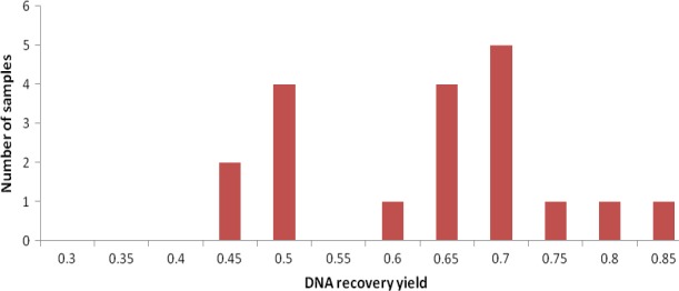
Distribution of the DNA recovery yield across the samples. For example, 2 samples had a DNA recovery yield between 0.4 and 0.45. The very large variation of the DNA recovery yields highlights the need of an internal standard to correct for this bias

4.3 qPCR data for the ratio E. coli/internal standard presented in Figure 2

Table A2.

Comparison between the number of E. coli cells added, the number of counts in the sequences and the conversion in the quantity of 16S rRNA genes E. coli per mg of feces. Since each E. coli cell possesses 7 copies of 16S rRNA genes, we would expect a 7 fold difference

QPCR method
Added Volume of E. coli suspension at 1.1 107 cells/µl (µl)	Added E. coli (cells)	Added E. coli (cells/mg_feces)	#counts of 16S genes from E. coli in the NGS data (sequences of E. coli out of 10808 sequences per sample)	Amount of 16S RNA genes of E. coli calculated with the help of the internal standard (copies 16S coli/mg)
0	0	0.00E+00	31 (95% Confidence interval 21–44)	1E+06
1	1E+07	8.38E+05	191 (95% Confidence interval 165–220)	6E+06
5	5E+07	4.39E+06	987 (95% Confidence interval 928–1,047)	5E+07
10	1E+08	7.90E+06	2,214 (95% Confidence interval 2,132–2,297)	9E+07
100	1E+09	8.65E+07	7,172 (95% Confidence interval 7,074–7,268)	8E+08

4.4 Absolute concentration of E. coli vs proportion in the 15 tubes

Figure A6.

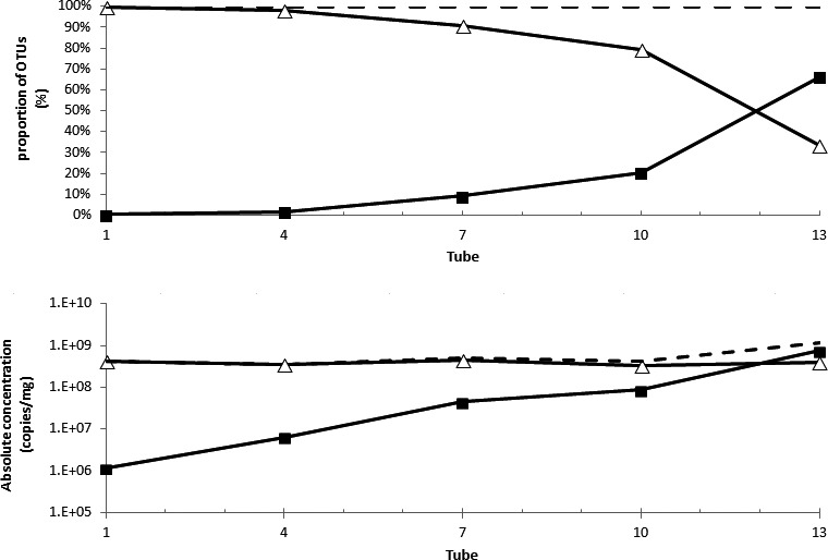
Proportion of E. coli (TOP) corresponding to the increase E. coli (BOTTOM). The black squares represent E. coli estimation after normalization by the DNA internal standard, the white triangles are the OTUs that are not E. coli. The total density is represented by the dotted line. The use of the DNA internal standard can determinate that the absolute concentration of E. coli increases (BOTTOM) rather than the classical image of the proportion of E. coli 16S rRNA sequences that varies (TOP)

This figure shows the potential difference in perception when reasoning in absolute concentration of bacterial population instead of mere proportions. We believe that absolute concentrations offer an edge for understanding the population dynamics.

5. Accuracy of the method with starving E. coli cells

In order to show that the method is accurate, we added the internal standard to resting DH10B E. coli cells grown in LB at 30°C for 7 days. The bacterial density was determined by plating, and was equal to 3.5 × 10⁸ ± 7 × 10⁷ coli/ml.

We then extracted 50 µl of this E. coli cell suspension using 750 µl of lysis buffer amended with 7 × 10⁵ copies of internal standard using the zymo fecal kit. The final elution volume was 50 µl. The measure was performed in duplicates to minimize pipeting errors.

Figure A7.

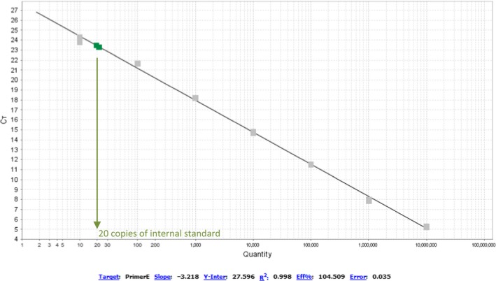
Measure of the internal standard with the help of primer pair E for stationary E. coli cells. We found 20.4 ± 1.5 copies of internal standard in the PCR reaction. Since the DNA was diluted 10 fold for the extraction and we had 50 µl of eluted DNA, this equals to 1.08 × 10⁴ copies found after extraction (out of 7 × 10⁵ copies of standard added to the 750 µl of lysis buffer used for each sample)

Figure A8.

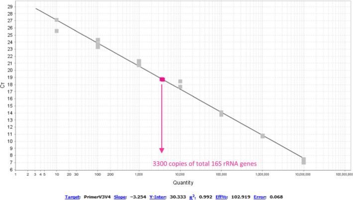
Measure of total copies of 16S rRNA (so this measure includes the internal standard) with the help of primer pair 334F/784R for stationary E. coli cells. We found 3296±146 copies of total rRNA genes in the PCR reaction. Since the DNA was diluted 10 fold for the extraction and we had 50 µl of eluted DNA, this equals to 1.13 10⁸ copies found after extraction (including 1.08 × 10⁴ copies of internal standard found after extraction)

To estimate the accuracy of the method, we used a sample of pure E. coli cells in stationary cells. For this particular experiment, we replaced the ratio usually obtained by NGS with the ratio obtained by qPCR.

Table A3.

Example of calculus of the density of starved E. coli cells using the internal standard with qPCR

Volume_added_coli_from_culture_in_stationary_phase (µl)	50
Added_coli_cells (since the suspension contains 3.5 × 108 coli/ml)	1.75E+07
Added_internal_standard (copies added via the lysis buffer)	7.00E+05
Quantity of the internal standard (qPCR primerE) (copies in the PCR tube)	20.4
Dilution_before_PCR	10
Volume_DNA_suspension	50
Recovered_standard (copies)	1.08E+04
DNA recovery yield	0.015
Quantity of all 16S rRNA (343F/784R which also target the internal standard) (copies in the PCR tube)	3296
Ratio of coli over total 16S fragments (usually determined by sequencing, here determined with the qPCR data because E. coli is the only species in the sample)	(3296–20.4)/3296 = 0.994
Number of 16S fragments belonging to E. coli (copies)	1.13E+08
Number of 16S copies per E. coli cell (information available from Picrust2 for any 16S sequence)	7
Estimated_coli_cells	1.47E+07
Precision of the method (estimated coli/added coli)	92%

In conclusion, taking into account the fact that E. coli has 7 copies of the 16S rRNA genes, we obtained 92 ± 11% of the cell count estimated by plating serial dilutions. The calculus illustrated above can be used in order to use the internal standard without NGS data if only a few species of interest are to be measured, and that qPCR primers are available for their quantification (the internal standard simply corrects for the variation in the DNA recovery yield during extraction). This result confirms that the finding of 8.9 copies of 16S rRNA genes per E.coli cell presented in the paper is not a mere artifact from the calibration of the method but indeed a result of residual growth.

6. Reproducibility of the quantification and error of the method

To show the reproducibility of the method, we extracted two 10mg‐samples in duplicates, and we measured quantities of total rRNA gene content corrected by the amount of the internal standard. The data below shows that the error of the method in such a case is <5%.

Table A4.

Reproductibility of the method to estimate the cell density with the qPCR of the internal standard and the total rRNA genes. The samples are extracted and measured separately. The precision of the method is below 5% error

		Sample 1 (replicate 1)	Sample 1 (replicate 2)	Sample 2 (replicate 1)	Sample 2 (replicate 2)
Metadata for qPCR method	weigth feces (mg)	10.1	10.5	10.5	9.9
	added_std (copies)	2.78E+07	2.78E+07	2.78E+07	2.78E+07
	added_std_per_mg	2.75E+06	2.65E+06	2.65E+06	2.81E+06
	Velution	100	100	100	100
	dilutionfactor	100	100	100	100
qPCR measurements	Std_Measure1 (compies/µlPCR)	17.5	17.8	17.4	17.3
	Std_Measure2 (compies/µlPCR)	17.4	18.5	17.3	17.3
	Std_Measure3 (compies/µlPCR)	17.2	17.3	17.3	17.1
	Std_in_tube (copies)	17,185.3	17,038.7	16,511.7	17,378.6
	efficiency	0.0	0.0	0.0	0.0
	total16S_Measure1 (copies/µl pcr)	17.9	16.8	17.9	16.7
	total16S_Measure2 (copies/µl pcr)	17.7	17.4	17.3	16.9
	total16S_Measure3 (copies/µl pcr)	17.6	18.0	17.7	16.7
	Quantity_16S (copies/µl pcr)	17.7	17.4	16793.5	16932.5
	Quantity_16S (copies_in_tube)	1.8E+05	1.7E+05	1.7E+08	1.7E+08
	Quantity_16S (copies/mg)	1.8E+04	1.7E+04	1.6E+07	1.7E+07
Estimation of the error between duplicates	average_between_replicates (copies/mg)	1.71E+04		1.65E+07
	std_dev_between_duplicates	6.98E+02		7.85E+05
	Error between replicate (in %)	4.1%		4.7%

Zemb O, Achard CS, Hamelin J, et al. Absolute quantitation of microbes using 16S rRNA gene metabarcoding: A rapid normalization of relative abundances by quantitative PCR targeting a 16S rRNA gene spike‐in standard. MicrobiologyOpen. 2020;9:e977 10.1002/mbo3.977

DATA AVAILABILITY STATEMENT

All sequences are available in NCBI GenBank under Bioproject PRJNA531076: https://www.ncbi.nlm.nih.gov/bioproject/531076. Supplemental information (such as the dada2 OTU table) can be found at https://doi.org/10.15454/YWMMH4

REFERENCES

- Aird, D. , Ross, M. G. , Chen, W.‐S. , Danielsson, M. , Fennell, T. , Russ, C. , … Gnirke, A. (2011). Analyzing and minimizing PCR amplification bias in Illumina sequencing libraries. Genome Biology, 12(2), R18 10.1186/gb-2011-12-2-r18 [DOI] [PMC free article] [PubMed] [Google Scholar]
- Baker, G. C. , Smith, J. J. , & Cowan, D. A. (2003). Review and re‐analysis of domain‐specific 16S primers. Journal of Microbiol Methods, 55(3), 541–555. 10.1016/j.mimet.2003.08.009 [DOI] [PubMed] [Google Scholar]
- Bremer, H. , & Dennis, P. P. (2008). Modulation of chemical composition and other parameters of the cell at different exponential growth rates. EcoSal Plus, 3(1). 10.1128/ecosal.5.2.3 [DOI] [PubMed] [Google Scholar]
- Callahan, B. J. , McMurdie, P. J. , Rosen, M. J. , Han, A. W. , Johnson, A. J. , & Holmes, S. P. (2016). DADA2: High‐resolution sample inference from Illumina amplicon data. Nature Methods, 13(7), 581–583. 10.1038/nmeth.3869 [DOI] [PMC free article] [PubMed] [Google Scholar]
- Dannemiller, K. C. , Lang‐Yona, N. , Yamamoto, N. , Rudich, Y. , & Peccia, J. (2014). Combining real‐time PCR and next‐generation DNA sequencing to provide quantitative comparisons of fungal aerosol populations. Atmospheric Environment, 84, 113–121. 10.1016/j.atmosenv.2013.11.036 [DOI] [Google Scholar]
- de Bruin, O. M. , & Birnboim, H. C. (2016). A method for assessing efficiency of bacterial cell disruption and DNA release. BMC Microbiology, 16(1), 197–197. 10.1186/s12866-016-0815-3 [DOI] [PMC free article] [PubMed] [Google Scholar]
- Falcioni, T. , Manti, A. , Boi, P. , Canonico, B. , Balsamo, M. , & Papa, S. (2006). Comparison of disruption procedures for enumeration of activated sludge floc bacteria by flow cytometry. Cytometry Part B: Clinical Cytometry, 70(3), 149–153. 10.1002/cyto.b.20097 [DOI] [PubMed] [Google Scholar]
- Fuentes, C. L. , & Arbeli, Z. (2007). Improved purification and PCR amplification of DNA from environmental samples. FEMS Microbiology Letters, 272(2), 269–275. 10.1111/j.1574-6968.2007.00764.x [DOI] [PubMed] [Google Scholar]
- Gonzalez, J. M. , Portillo, M. C. , Belda‐Ferre, P. , & Mira, A. (2012). Amplification by PCR artificially reduces the proportion of the rare biosphere in microbial communities. PLoS ONE, 7(1), e29973 10.1371/journal.pone.0029973 [DOI] [PMC free article] [PubMed] [Google Scholar]
- Hardwick, S. A. , Chen, W. Y. , Wong, T. , Kanakamedala, B. S. , Deveson, I. W. , Ongley, S. E. , … Mercer, T. R. (2018). Synthetic microbe communities provide internal reference standards for metagenome sequencing and analysis. Nature Communications, 9(1), 3096 10.1038/s41467-018-05555-0 [DOI] [PMC free article] [PubMed] [Google Scholar]
- Ipharraguerre, I. R. , Pastor, J. J. , Gavaldà‐Navarro, A. , Villarroya, F. , & Mereu, A. (2018). Antimicrobial promotion of pig growth is associated with tissue‐specific remodeling of bile acid signature and signalling. Scientific Reports, 8(1), 13671 10.1038/s41598-018-32107-9 [DOI] [PMC free article] [PubMed] [Google Scholar]
- Jackson, D. A. (1997). Compositional data in community ecology: The paradigm or peril of proportions? Ecology, 78(3), 929–940. 10.1890/0012-9658(1997)078[0929:cdicet]2.0.co;2 [DOI] [Google Scholar]
- Kumar, M. S. , Slud, E. V. , Okrah, K. , Hicks, S. C. , Hannenhalli, S. , & Corrada Bravo, H. (2018). Analysis and correction of compositional bias in sparse sequencing count data. BMC Genomics, 19(1), 799 10.1186/s12864-018-5160-5 [DOI] [PMC free article] [PubMed] [Google Scholar]
- Lee, T. J. , Wong, J. , Bae, S. , Lee, A. J. , Lopatkin, A. , Yuan, F. , & You, L. (2015). A power‐law dependence of bacterial invasion on mammalian host receptors. Plos Computational Biology, 11(4), e1004203 10.1371/journal.pcbi.1004203 [DOI] [PMC free article] [PubMed] [Google Scholar]
- Magoc, T. , & Salzberg, S. L. (2011). FLASH: Fast length adjustment of short reads to improve genome assemblies. Bioinformatics, 27(21), 2957–2963. 10.1093/bioinformatics/btr507 [DOI] [PMC free article] [PubMed] [Google Scholar]
- Morton, J. T. , Marotz, C. , Washburne, A. , Silverman, J. , Zaramela, L. S. , Edlund, A. , … Knight, R. (2019). Establishing microbial composition measurement standards with reference frames. Nature Communications, 10(1), 2719 10.1038/s41467-019-10656-5 [DOI] [PMC free article] [PubMed] [Google Scholar]
- Piwosz, K. , Shabarova, T. , Tomasch, J. , Šimek, K. , Kopejtka, K. , Kahl, S. , … Koblížek, M. (2018). Determining lineage‐specific bacterial growth curves with a novel approach based on amplicon reads normalization using internal standard (ARNIS). ISME Journal, 12(11), 2640–2654. 10.1038/s41396-018-0213-y [DOI] [PMC free article] [PubMed] [Google Scholar]
- Props, R. , Kerckhof, F. M. , Rubbens, P. , De Vrieze, J. , Hernandez Sanabria, E. , Waegeman, W. , … Boon, N. (2017). Absolute quantification of microbial taxon abundances. ISME Journal, 11(2), 584–587. 10.1038/ismej.2016.117 [DOI] [PMC free article] [PubMed] [Google Scholar]
- Rastelli, M. , Knauf, C. , & Cani, P. D. (2018). Gut Microbes and health: A focus on the mechanisms linking microbes, obesity, and related disorders. Obesity (Silver Spring, Md.), 26(5), 792–800. 10.1002/oby.22175 [DOI] [PMC free article] [PubMed] [Google Scholar]
- Ruijter, J. M. , Ramakers, C. , Hoogaars, W. M. , Karlen, Y. , Bakker, O. , van den Hoff, M. J. , & Moorman, A. F. (2009). Amplification efficiency: Linking baseline and bias in the analysis of quantitative PCR data. Nucleic Acids Research, 37(6), e45 10.1093/nar/gkp045 [DOI] [PMC free article] [PubMed] [Google Scholar]
- Stämmler, F. , Gläsner, J. , Hiergeist, A. , Holler, E. , Weber, D. , Oefner, P. J. , … Spang, R. (2016). Adjusting microbiome profiles for differences in microbial load by spike‐in bacteria. Microbiome, 4(1), 28 10.1186/s40168-016-0175-0 [DOI] [PMC free article] [PubMed] [Google Scholar]
- Sun, Y. J. , Cai, Y. P. , Huse, S. M. , Knight, R. , Farmerie, W. G. , Wang, X. Y. , & Mai, V. (2011). A large‐scale benchmark study of existing algorithms for taxonomy‐independent microbial community analysis. Briefings in Bioinformatics, 13(1), 107–121. 10.1093/bib/bbr009 [DOI] [PMC free article] [PubMed] [Google Scholar]
- Tkacz, A. , Hortala, M. , & Poole, P. S. (2018). Absolute quantitation of microbiota abundance in environmental samples. Microbiome, 6(1), 110 10.1186/s40168-018-0491-7 [DOI] [PMC free article] [PubMed] [Google Scholar]
- Vandamme, P. , & Coenye, T. (2003). Intragenomic heterogeneity between multiple 16S ribosomal RNA operons in sequenced bacterial genomes. FEMS Microbiology Letters, 228(1), 45–49. 10.1016/S0378-1097(03)00717-1 [DOI] [PubMed] [Google Scholar]
- Vandeputte, D. , Kathagen, G. , D'Hoe, K. , Vieira‐Silva, S. , Valles‐Colomer, M. , Sabino, J. , … Raes, J. (2017). Quantitative microbiome profiling links gut community variation to microbial load. Nature, 551(7681), 507–511. 10.1038/nature24460 [DOI] [PubMed] [Google Scholar]
- Venkataraman, A. , Parlov, M. , Hu, P. , Schnell, D. , Wei, X. , & Tiesman, J. P. (2018). Spike‐in genomic DNA for validating performance of metagenomics workflows. BioTechniques, 65(6), 315–321. 10.2144/btn-2018-0089 [DOI] [PubMed] [Google Scholar]
- Verschuren, L. M. G. , Calus, M. P. L. , Jansman, A. J. M. , Bergsma, R. , Knol, E. F. , Gilbert, H. , & Zemb, O. (2018). Fecal microbial composition associated with variation in feed efficiency in pigs depends on diet and sex. Journal of Animal Science, 96(4), 1405–1418. 10.1093/jas/sky060 [DOI] [PMC free article] [PubMed] [Google Scholar]
- Vishnivetskaya, T. A. , Layton, A. C. , Lau, M. C. , Chauhan, A. , Cheng, K. R. , Meyers, A. J. , … Onstott, T. C. (2014). Commercial DNA extraction kits impact observed microbial community composition in permafrost samples. FEMS Microbiology Ecology, 87(1), 217–230. 10.1111/1574-6941.12219 [DOI] [PubMed] [Google Scholar]
- Werner, J. J. , Koren, O. , Hugenholtz, P. , DeSantis, T. Z. , Walters, W. A. , Caporaso, J. G. , … Ley, R. E. (2012). Impact of training sets on classification of high‐throughput bacterial 16s rRNA gene surveys. The ISME Journal, 6(1), 94–103. 10.1038/ismej.2011.82 [DOI] [PMC free article] [PubMed] [Google Scholar]
- Yuan, S. , Cohen, D. B. , Ravel, J. , Abdo, Z. , & Forney, L. J. (2012). Evaluation of methods for the extraction and purification of DNA from the human microbiome. PLoS ONE, 7(3), e33865–e33865. 10.1371/journal.pone.0033865 [DOI] [PMC free article] [PubMed] [Google Scholar]
Associated Data
This section collects any data citations, data availability statements, or supplementary materials included in this article.