Multiple Free Energy Calculations from Single State Point Continuous Fractional Component Monte Carlo Simulation Using Umbrella Sampling

Abstract

We introduce an alternative method to perform free energy calculations for mixtures at multiple temperatures and pressures from a single simulation, by combining umbrella sampling and the continuous fractional component Monte Carlo method. One can perform a simulation of a mixture at a certain pressure and temperature and accurately compute the chemical potential at other pressures and temperatures close to the simulation conditions. This method has the following advantages: (1) Accurate estimates of the chemical potential as a function of pressure and temperature are obtained from a single state simulation without additional postprocessing. This can potentially reduce the number of simulations of a system for free energy calculations for a specific temperature and/or pressure range. (2) Partial molar volumes and enthalpies are obtained directly from the estimated chemical potentials. We tested our method for a Lennard-Jones system, aqueous mixtures of methanol at T = 298 K and P = 1 bar, and a mixture of ammonia, nitrogen, and hydrogen at T = 573 K and P = 800 bar. For pure methanol (N = 410 molecules), we observed that the estimated chemical potentials from umbrella sampling are in excellent agreement with the reference values obtained from independent simulations, for ΔT = ±15 K and ΔP = 100 bar (with respect to the simulated system). For larger systems, this range becomes smaller because the relative fluctuations of energy and volume become smaller. Without sufficient overlap, the performance of the method will become poor especially for nonlinear variations of the chemical potential.

1. Introduction

Knowledge of chemical potentials is essential for understanding and studying phase behavior of multicomponent systems.^1,2 In Monte Carlo (MC) simulations, chemical potentials cannot be easily computed from a single simulation because chemical potentials cannot be expressed directly as a function of phase space variables (coordinates and momenta).³⁻⁶ One of the most straightforward and commonly used methods to compute the chemical potentials is Widom’s test particle insertion (WTPI) method.^4,7,8 In this method, test particles are inserted at randomly selected positions inside the simulation box. The chemical potential is computed by sampling the interaction energies of the test particles with the other molecules in the system. In the NPT ensemble, the chemical potential of a certain component in a mixture is obtained from

1

in which ⟨···⟩ indicates an ensemble average, A is the component type, β = (k_BT)⁻¹, and k_B is the Boltzmann constant. V and T are the volume and temperature of the system, respectively. ΔU^A+ is the interaction energy of the test molecule of type A with the rest of the molecules. The partial molar volume and enthalpy of component type A can be written as derivatives of μ_A,⁹ namely, h̅ = (∂(βμ)/∂β)_P and υ̅ = (∂μ/∂P)_T.^9,10 In their pioneering work in the 80s of the past century, Frenkel et al. developed a method based on the WTPI method to compute partial molar properties.^11,12 These properties cannot be directly written as averages of phase space variables. Frenkel et al. showed that by random insertions of a test particle, partial molar properties (in the NPT ensemble) are obtained from¹¹

2a

2b

in which N denotes the number of molecules in the system and s denotes the scaled coordinates. In the case of an ideal gas, h̅_A^ex in eq 2a becomes zero because there are no intermolecular interaction between the molecules. The derivation of eqs 2a and 2b is shown in detail in our earlier work.¹⁰ Partial molar properties are important for studying thermodynamic properties of multicomponent mixtures. Partial molar enthalpies also play a role in nonequilibrium thermodynamics, for example, in studying the heat flux in mixtures.¹¹ Recently, Josephson, Siepmann, and co-workers introduced a method to compute partial molar properties in the NPT version of the Gibbs ensemble using a method based on postprocessing fluctuations in energy, volume, and the number of molecules of each component.¹³ It is also possible to compute partial molar properties from Kirkwood–Buff integrals.¹⁴⁻²⁰ In our recent work, we have outlined the importance of computing partial molar volumes υ̅ and partial molar enthalpies h̅ and provided an overview of different methods developed for computing partial molar properties in molecular simulation studies.¹⁰ Similar to eq 1, efficient sampling of partial molar properties using eqs 2a and 2b relies on the formation of cavities in the system, sufficiently large for a test particle. The probability of formation of such cavities is directly related to the density of the system. The limitations of insertion/deletion type methods are well-known for dense systems and/or systems with complex molecules.^4,10,21−26 At high density, test particle insertions result in overlaps with existing molecules in the system, leading to a very large potential energy ΔU^A+, that is, a very small Boltzmann factor as shown in eqs 1, 2a and 2b. Because of increased computational power since the early 1950s,²⁷⁻²⁹ more complex systems have been investigated in molecular simulation studies of phase equilibria.³⁰⁻³³ The inherent limitations of the WTPI method in free energy calculations in complex systems have led to the development of other simulation methods.^7,8,34

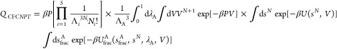
In the previous century, alternative methods were introduced to circumvent the sampling problems of the WTPI method, such as the overlapping distribution method (ODM) by Bennett³⁵ or combining particle insertion and deletion methods by Shing and Gubbins.³⁶⁻³⁸ The ODM is based on the free energy difference between two systems. This computation is not efficient if the systems significantly differ in configuration space.^7,25 Other Widom-type methods such as the Theodorou deletion method²² and Widom’s test particle deletion method²¹ suffer from the same sampling difficulties associated with the WTPI method for complex and dense systems.³⁹ Lyubartsev et al. developed expanded ensembles for accurate free energy calculations of complex systems.³ This method takes advantage of gradual insertion/deletion of molecules which allows the system to gradually adjust to the new configuration in which a new molecule is added.⁴⁰⁻⁴⁶ Inspired by this, Shi and Maginn developed the continuous fractional component MC (CFCMC) method to facilitate molecule exchanges in open ensemble simulation of dense phases.⁴⁷ In CFCMC simulations, a fractional molecule is added to the ensemble. During the simulation, the interactions of this molecule are adjusted with a coupling parameter (λ). The fractional molecule acts as ideal gas if λ = 0 and interacts fully with other molecules if λ = 1. The application of the CFCMC method for systems ranging from Lennard-Jones (LJ) particles to larger molecules such as hydrocarbons is well-established, see refs (48) and (49). Although the method by Shi and Maginn facilitates molecule exchanges in dense phases, postprocessing is required to obtain the chemical potentials. Recently, Vlugt and co-workers combined the CFCMC method with free energy calculations in ref (2). In this method (hereafter referred to as the CFCMC method), the chemical potential can be directly computed by sampling the probability distribution p(λ). Consider a multicomponent mixture of mono-atomic components, expanded with a fractional molecule. In the NPT ensemble, the ensemble partition function can be written as^10,50

3

in which U_frac^A is the interaction energy of the fractional molecule. Depending on the value of λ, U_frac can vary between “zero” and “fully scaled”.^1,1,47,51 The chemical potential of component A in CFCNPT equals⁵⁰

4

in which ρ_A is the number density of A. To make the logarithm in eq 4 dimensionless, an arbitrary reference density ρ₀ is selected. The term μ₀ contains intramolecular contributions to the chemical potential. p(λ_A = 1) and p(λ_A = 0) are the probabilities of λ_A when λ_A = 1 and λ_A = 0, respectively. The chemical potential of eq 4 is split into an ideal gas part and excess part. It is shown in ref (10) that the computed chemical potentials obtained using eqs 1 and 4 are the same by definition. In the CFCNPT ensemble, the partial molar excess enthalpy and partial molar volume are equal¹⁰

5a

5b

in which ⟨H⟩ and ⟨V⟩ are ensemble averages of the total enthalpy and total volume computed at λ_A = 1 and ⟨H/V⟩ and ⟨1/V⟩ are ensemble averages computed at λ_A = 0. In ref (10), we showed that eqs 2a, 2b, 5a, and 5b are identical and yield identical results. Because the intramolecular contribution is not included in Q_CFCNPT of eq 3, the excess partial molar enthalpy computed using eq 5a is always taken with respect to the ideal gas. Because the WTPI method suffers at high densities, the application of eqs 1, 2a, and 2b is rather limited, in sharp contrast to eqs 4, 5a, and 5b. In our recent publications, the advantages of using the CFCMC method for free energy calculations are shown for various systems.^{1,2,10,52−55} To further use the CFCMC method, we introduce a formulation, based on the idea of umbrella sampling,⁵⁶ allowing one to compute the chemical potentials (eq 4) for multiple state points from a single state point simulation.

Umbrella sampling is a well-known method developed by Torrie and Valleau⁵⁶ from which the free energy difference between the system of interest and a reference system can be obtained.^7,34,56 By introducing a biasing function , the ensemble average ⟨A⟩ in the canonical ensemble is calculated from an ensemble where the configuration space is sampled proportional to

6

in which ⟨···⟩_Π denotes an ensemble average in the ensemble Π. The biasing function is only a function of the configuration space. The derivation is provided in ref (34). In this paper, we show that by combining eq 6 with CFCMC, the chemical potentials can be accurately estimated for an appreciable temperature and pressure range from a single state simulation in the CFCNPT ensemble. To estimate the chemical potential at a temperature or pressure different from that of the simulation, sufficient overlap is required between the configuration space of the two systems.^7,34 This depends also on the system size. The relative density and energy fluctuations become smaller with the increase in system size, which may reduce the overlap between the configuration spaces of two systems. Therefore, we investigated the limitations of combining umbrella sampling with the CFCMC method when estimating chemical potentials for various temperature and pressure intervals. The combination of umbrella sampling with the CFCMC method offers the following advantages: (1) Accurate estimates of the chemical potential as a function of pressure or temperature are computed from a single simulation. (2) Partial molar properties are obtained directly from a single simulation. By definition, partial molar properties can be obtained by numerically evaluating the expressions h̅ = (∂(βμ)/∂β)_P and υ̅ = (∂μ/∂P)_T, using the estimated chemical potentials at different pressures and temperatures.^9,10 (3) Partial molar enthalpies obtained from umbrella sampling can be used as an independent check for the CFCMC method in eqs 5a and 5b, both for programming bugs or an independent check whether the phase space is sufficiently sampled.

In Section 2, the combination of umbrella sampling and free energy calculations in CFCMC simulations is explained. In Section 3, we provide a detailed overview of the systems considered in our simulations. In Section 4, our simulation results are presented. In this section, the chemical potentials for a binary LJ color mixture are estimated at multiple temperatures and pressures by performing single state simulations in the CFCNPT ensemble. The results from umbrella sampling are in excellent agreement with the ones obtained from independent simulations. In addition, partial molar properties are estimated by numerically evaluating h̅ = (∂(βμ)/∂β)_P and υ̅ = (∂μ/∂P)_T, based on the results from umbrella sampling. The computed partial molar properties for the LJ mixture are in excellent agreement with the results from the CFCMC method (eqs 5a and 5b) and the WTPI method (eqs 2a and 2b). As an example of a molecular system, we applied our method to different mixtures of water and methanol at standard conditions (T = 298 K and P = 1 bar) and compared the results with those obtained from independent CFCNPT simulations. Accurate estimates of the chemical potential of water and methanol are obtained using umbrella sampling for a temperature difference ΔT = ±10 K, for N = 470 molecules. Excellent agreement is observed between partial molar properties of water and methanol obtained from umbrella sampling and those obtained using eqs 5a and 5b. We also applied our method to a mixture of ammonia, nitrogen, and hydrogen at T = 573 K and P = 800 bar at chemical equilibrium and compared the partial molar properties obtained from our method to those obtained from the CFCMC method. The limitations of the method are tested by decreasing overlap in configuration space for pure methanol. In Section 5, our conclusions are presented.

2. Theory

Similar to eq 6, we combine umbrella sampling with the CFCMC method to estimate the probability distribution p(λ) at (T, P^★) while performing a simulation at (T^★, P^★) in the CFCNPT ensemble. This distribution is calculated using

7

in which H = U + PV, U is the internal energy of the system, and c is a normalization constant. In the ensemble, at β*, the value of the scaling parameter equals λ′. In the Supporting Information, one can find the derivation of eq 7. To estimate the excess part of the chemical potential in eq 4 at β, the values p(λ = 1)|_β and p(λ = 0)|_β are obtained using eq 7. Similar to eq 7, it can be shown that the number density can be calculated at T* using

8

in which ρ_N|_β is the number density at β. The number of fractional molecules is not included in computing number densities.¹ If the number of fractional molecules is much smaller compared to that of the whole molecules (less than 1%), Boltzmann averages are not affected.⁵⁰ By combining eqs 4, 7, and 8, the chemical potential at (T, P^★) is estimated while performing a single simulation at (T^★, P^★). In a similar manner, the distribution p(λ) at (T^★, P) can be estimated while performing a simulation at (T^★, P^★), keeping the number of molecules constant. This distribution is obtained by introducing a bias to the ensemble average

9

The derivation of eq 9 can be found in the Supporting Information. By computing the values p(λ = 0)|_P and p(λ = 1)|_P based on eq 9, one can obtain the excess chemical potential at pressure P while performing a simulation at pressure P^★. For the ideal part of the chemical potential in eq 4, the number density is estimated at P using umbrella sampling

10

By combining eqs 4, 9, and 10, the chemical potential at (T^★, P) is obtained while performing a single state simulation at (T^★, P^★). The derivation of eq 10 is very similar to the derivation of eq 9.

3. Simulation Details

Besides thermalization trial moves in the CFCNPT ensemble, three additional sorts of trial moves are defined to facilitate gradual insertions/deletions of the fractional molecule: (1) changes in λ: randomly increasing or decreasing λ while the positions and orientations of all molecules are fixed. For the fractional molecule, the LJ interactions are scaled using^57,58

11

It is possible to choose different alchemical pathways for u_LJ. A detailed study of different alchemical pathways can be found in refs (57−59). For details on scaling, how the electrostatic interactions are scaled, the reader is referred to refs (1, 52, 55). (2) Identity changes: an attempt is made to transform the fractional molecule into a whole molecule and simultaneously transform a randomly selected whole molecule into a fractional molecule. (3) Random re-insertions: the fractional molecule is re-inserted at a randomly selected position. Except for the fractional molecule, orientations and positions of other molecules do not change. The acceptance rules for these trial moves are derived based on metropolis importance sampling.^1,27 The trial move (2) has a high acceptance probability at high values of λ, and the trial move (3) has a high acceptance probability at low values of λ. Therefore, it is efficient to combine trial moves (2) and (3) and use a single hybrid trial move.^1,10 It is shown in ref (10) that combining the last two trial moves leads to higher acceptance ratios of trial moves (2) and (3). To flatten the λ space, prior to performing production runs, a weight function W(λ) was computed using the Wang–Landau (WL) algorithm.^60,61

To demonstrate the feasibility of our method, MC simulations were carried out to compute the chemical potentials of an LJ color mixture (50–50%) in the CFCNPT ensemble, containing N = 200 molecules. All simulations were carried out at T* = 2 and pressures between P* = 0.1 and P* = 8 (the symbol * denotes the reduced units). For the LJ system, eqs 7 and 8 were used to compute the chemical potential at temperatures between T* = 1.82 and T* = 2.22 and a pressure of P* = 6 from a single simulation at (T* = 2, P* = 6). Similarly, eqs 9 and 10 were used to compute the chemical potentials at T* = 2 and pressures between P* = 5.95 and P* = 6.05 in the same simulation. To compute the reference values for the chemical potentials, independent simulations were performed for each temperature and pressure. The estimated chemical potentials obtained from umbrella sampling were used to numerically evaluate the partial molar properties using the expressions h̅ = (∂(βμ)/∂β)_P and υ̅ = (∂μ/∂P)_T. As a reference, the partial molar properties were also computed using the WTPI method using eqs 2a and 2b and the CFCMC method using eqs 5a and 5b. All LJ interactions were truncated and shifted at 2.5σ, and the thermal wavelength Λ was set to unity. For every simulation of the LJ system in the CFCNPT ensemble, 10⁵ cycles were used for equilibration and 10⁷ cycles were used for production. The number of trial moves in each cycle is equal to the total number of molecules in the system. The following probabilities were set for selecting trial moves: 33% translations, 33% λ changes, 33% hybrid trial moves, and 1% volume changes.

To test this method for a more complex system, aqueous methanol mixtures with mole fractions of methanol between x_MeOH = 0.2 and x_MeOH = 0.8 were simulated in the CFCNPT ensemble. All MC simulations were performed using our in-house code. We verified that the same results were obtained for various systems^1,52 when the RASPA software package^62,63 was used. For water, the TIP4P/2005⁶⁴ and for methanol, the TraPPE⁶⁵ force fields were used. Sites with a partial charge but no LJ parameters are protected by adding an LJ site with ϵ/k_B = 1 K and σ = 1 Å. A comparison between different combinations of force fields for predicting thermodynamic properties of aqueous methanol mixtures is provided in our earlier work.⁵⁵ In all simulations of water–methanol mixtures, a fractional molecule of methanol and a fractional molecule of water were present. All molecules were modeled as rigid objects, and pairwise interaction potentials consisted only of LJ and Coulomb potentials. A cutoff radius of 12 Å for both LJ and Coulomb potentials was used. Lorentz–Berthelot was used for cross interactions between methanol and water molecules, and analytic tail corrections were applied.^7,8 The damped shifted force method⁶⁶ is used to handle the electrostatic interactions of water and methanol systems. For details on using these cutoff-based methods, the reader is referred to refs (52, 55, 66−69). The interactions of the fractional molecule are scaled in the following way: starting from λ = 1, the electrostatic interactions are scaled to zero and thereafter the LJ interactions are scaled to zero. This circumvents configurations with charge overlaps between the fractional molecule and other molecules leading to numerical instabilities in the simulation.^{57−59,70−72} Chemical potentials of water and methanol between T = 288 K and T = 308 K were estimated by performing umbrella sampling from a single simulation of the water–methanol mixture at T = 298 K and P = 1 bar. As a reference, the chemical potentials of water and methanol were computed independently at every pressure and temperature. Subsequently, partial molar properties of water and methanol were obtained from the estimated chemical potentials using umbrella sampling. The results were compared to the partial molar properties obtained using eqs 5a and 5b.¹⁰ For every simulation of the water–methanol system in the CFCNPT ensemble, 10⁵ cycles were used for equilibration and 6 × 10⁶ cycles for production. The following probabilities were set for selecting trial moves: 35% translations, 30% rotations, 17% λ changes, 17% hybrid trial moves, and 1% volume changes. The WL algorithm^60,61 was used independently for water and methanol to flatten the probability of λ.^60,61 In ref (50), we showed that the correlation between scaling parameters of different fractional molecules is weak and independent of the weight function. It is therefore computationally advantageous to separate the multidimensional weight function into a series of one dimensional weight functions: W(λ₁, λ₂) ≈ W(λ₁) + W(λ₂). This is due to the fact that filling one-dimensional histograms is more efficient than filling two separate multidimensional histograms.⁵⁰ To investigate the limitations of umbrella sampling in CFCMC simulations, umbrella sampling was applied to estimate the chemical potentials of pure methanol for a wide pressure and temperature range. The results were compared to the results obtained from independent simulations of pure methanol in the CFCNPT ensemble, at every temperature and pressure.

To compute partial molar properties of ammonia, nitrogen, and hydrogen in their mixture at T = 573 K and P = 800 bar, simulations were performed in the CFCNPT ensemble.¹⁰ Similar to our previous work, separate simulations were performed in which only a single fractional molecule was present. This was repeated for the three components, leading to three independent simulations. Force field and simulation details are provided in ref (10). The starting mixture composition (N_NH3 = 407, N_N2 = 7, and N_H2 = 20) was obtained from simulations of the Haber–Bosch process in the reaction ensemble as described in ref (1).

4. Results and Discussion

A simulation in the CFCNPT ensemble was performed for an LJ system at T* = 2 and P* = 6. Using umbrella sampling, the chemical potentials were computed for temperatures ranging from T* = 1.82 to T* = 2.22 and pressures ranging from P* = 5.95 to P* = 6.05. The values of the chemical potential were compared to those obtained from independent CFCNPT simulations for all temperatures and pressures. The results are shown in Table 1. Excellent agreement is observed between the computed chemical potentials obtained using umbrella sampling from a single simulation at (T* = 2, P* = 6) and the chemical potentials calculated from independent simulations at P* = 6 and temperatures between T* = 1.82 and T* = 2.22. In this work, the error bars (uncertainties) are obtained by computing the standard deviation of the mean from five independent simulations. It should be noted that the uncertainty of the computed chemical potential associated with umbrella sampling increases with the increase in the temperature difference |ΔT*|. Because the overlap between the configuration spaces decreases with the increase in temperature or pressure difference, it impairs the sampling. The overlap between the configuration spaces also decreases with the increase in system size, as the relative fluctuations of energy and volume become smaller for larger systems. In Table 1b, the estimated chemical potentials from umbrella sampling from a single simulation at (T* = 2, P* = 6) are compared to the chemical potentials obtained from independent simulations at T* = 2 and pressures between P* = 5.95 and P* = 6.05. Excellent agreement is observed between the computed chemical potentials estimated using umbrella sampling and the results obtained from independent simulations for the entire pressure range. From the results presented in Table 1, it can be observed that accurate estimates of the chemical potentials are obtained from a single simulation combining the CFCMC method with umbrella sampling. Although the statistical uncertainties of the estimated chemical potentials obtained from umbrella sampling are larger compared to those obtained from independent simulations, the differences in uncertainties are not significant.

Table 1. Chemical Potentials for a Binary (50–50%) LJ Mixture Obtained from Umbrella Sampling (Eqs 7 and 9) and Independent Simulations in the CFCNPT Ensemble (Eq 4)^a.

^aTo obtain estimates of the chemical potentials at (a) different temperatures and (b) pressures, umbrella sampling is performed at T* = 2 and P* = 6 in a single simulation. Boltzmann averages at T* = 2 and P* = 6 are highlighted in gray. Numbers in brackets indicate uncertainties.

The chemical potentials obtained from umbrella sampling are used to compute the partial molar properties for the LJ mixture, by numerically differentiating (∂(βμ)/∂β)_P and (∂μ/∂P)_T. For instance, the chemical potentials shown in Table 1 are used to plot βμ–β and μ–P for T* = 2 and P* = 6, as shown in Figure 1. The data points connected with a line as shown in Figure 1 indicate that the data points were obtained from a single simulation combining CFCMC and umbrella sampling, and the individual data points were obtained from independent CFCNPT simulations. Calculating the slopes as shown in Figure 1, at T* = 2 and P* = 6, leads to the values of the partial molar volumes and enthalpies. A central difference scheme with high order approximation was used to compute the partial molar enthalpies as shown in Figure 1a and partial molar volumes as shown in Figure 1b. The partial molar excess enthalpy was computed by subtracting the ideal gas contribution from the total partial molar enthalpy. It is shown in ref (10) that the ideal part of the partial molar enthalpy of an LJ particle, h̅^id equals 5/(2β). It is noteworthy that the contribution of the thermal wavelength Λ in h̅^id equals 3/(2β).¹⁰ Because Λ is set to unity in our simulations, the contribution of the thermal wavelength cancels out when numerically evaluating (∂(βμ)/∂β)_P. Therefore, the partial molar excess enthalpy is obtained from umbrella sampling of the chemical potential using h̅^ex = (∂(βμ)/∂β)_P – 1/β. The partial molar properties for the LJ system obtained from umbrella sampling and the CFCMC method (eqs 5a and 5b) and the WTPI method (eqs 2a and 2b) are provided in Table 2. Excellent agreement is observed between the partial molar properties from CFCNPT simulations and the results obtained from umbrella sampling. Similar uncertainties are observed between the two methods. For the LJ system, umbrella sampling works equally well compared to the CFCMC method. In addition, accurate estimates of the chemical potential at different pressures and temperatures are obtained without any extra computational power or post processing.

Figure 1.

Plots showing (a) β*μ–β* and (b) μ–P* for an LJ binary color mixture consisting of 200 molecules. Downward-pointing triangles indicate the results obtained from independent CFCNPT simulations at pressures between P* = 5.94 and P* = 6.05 and temperatures between T* = 1.82 and T* = 2.22. Circles indicate the results obtained by performing umbrella sampling from a single simulation in the CFCNPT ensemble at T* = 2 and P* = 6. Lines indicate that the data are obtained from a single simulation. Error bars are smaller than the symbol sizes. Raw data are listed in Table 1.

Table 2. Densities, Chemical Potentials, Partial Molar Excess Enthalpies, and Volumes at T* = 2 and Pressures between P* = 0.1 and P* = 8 Computed for a Binary LJ Color Mixture (200 Molecules)^a.

			CFCNPT		umbrella sampling		WTPI method
P*	⟨ρ*⟩	μA	h̅Aex	υ̅A	h̅Aex	υ̅A	h̅Aex	υ̅A
0.1	0.052	–7.460(7)	–0.44(4)	18.6(3)	–0.44(5)	19(2)	–0.361(5)	19.29(4)
2	0.584	–1.075(8)	–1.6(1)	1.72(3)	–1.6(1)	1.72(3)	–1.64(4)	1.70(1)
4	0.722	1.957(5)	–0.06(5)	1.39(1)	–0.06(5)	1.39(1)	–0.3(2)	1.36(5)
6	0.800	4.581(9)	1.7(2)	1.26(2)	1.7(2)	1.26(2)	1.6(8)	1.23(5)
8	0.856	7.001(6)	3.2(1)	1.17(1)	3.2(1)	1.17(1)	4(1)	1.2(1)

^aThree different methods are used at each P*, in order to compare the results for the partial molar properties: the WTPI method (eqs 2a and 2b) in the NPT ensemble,^11,12 the CFCMC method (in the CFCNPT ensemble, eqs 5a and 5b),¹⁰ and umbrella sampling (eqs 7 and 9). The chemical potentials are calculated using eq 4 from independent simulations. Numbers in brackets indicate uncertainties.

Other realistic systems with complex intermolecular interactions considered here are different aqueous methanol mixtures with mole fractions of methanol between x_MeOH = 0.2 and x_MeOH = 1. These systems were simulated in the CFCNPT ensemble. For a mixture composition x_MeOH = 0.8, umbrella sampling was used to estimate the chemical potentials of water and methanol at temperatures between T = 288 K and T = 308 K while running a single CFCNPT simulation at P = 1 bar and T = 298 K. In addition, independent simulations in the CFCNPT simulations were performed to obtain the chemical potentials as a reference. The results are shown in Table 3. Accurate estimates of the chemical potentials of water and methanol are obtained between T = 288 K and T = 308 K, from a single CFCNPT simulation T = 298 K (ΔT = ±10 K). The relative differences between the estimates of the chemical potentials and the chemical potentials obtained from independent simulations are well below 1%. For each temperature, the differences between the absolute values of the chemical potentials as shown in Table 3 are significantly smaller than 1 kcal/mol = 4.184 kJ/mol, which is typically considered as a benchmark in the computational chemistry literature.⁷³ The results show that umbrella sampling can provide an accurate estimate of the chemical potentials of water and methanol for an appreciable temperature range (around ΔT = ±10 relative to the simulation temperature). The raw data shown in Table 3 were used to plot βμ as a function of β for the water–methanol mixture (N = 470), x_MeOH = 0.8, at temperatures between T = 288 K and T = 308 K. The results are shown in Figure 2. The lines indicate data obtained from a single simulation. It can be seen in Figure 2 that excellent agreement is observed between the results obtained from umbrella sampling and the reference values from independent simulations in CFCNPT at every temperature. The error bars associated with the estimated chemical potentials for water and methanol increase with increase in |ΔT| relative to T = 298 K. This indicates that umbrella sampling becomes inefficient and inaccurate for a larger temperature difference. It should be emphasized that this temperature range is not a priori known and is system- and system size-dependent. We explain later in this paper how a reasonable temperature or pressure range can be selected for umbrella sampling of the chemical potentials.

Table 3. Chemical Potentials [kJ/mol] of the Water–Methanol Mixtures (x_MeOH = 0.8) Obtained from Umbrella Sampling and Independent Simulations in the CFCNPT Ensemble at Temperatures between T = 288 K and T = 308 K^a.

^aThe values of the chemical potentials are estimated using umbrella sampling at T = 298 K and P = 1 bar. The corresponding Boltzmann averages are highlighted in gray. Numbers in brackets indicate uncertainties.

Figure 2.

Plot showing βμ–β for a water–methanol mixture, x_MeOH = 0.8. To compute the chemical potentials, independent simulations are performed at temperatures between T = 288 K and T = 308 K. Downward-pointing triangles and upward-pointing triangles denote data for water and methanol from independent CFCNPT simulations. Asterisks connected by a line indicate data obtained using umbrella sampling from a single simulation at T = 298 K and P = 1 bar. Error bars are smaller than the symbol sizes. Raw data are listed in Table 3.

The βμ–μ and μ–P plots for the water–methanol mixture at x_MeOH = 0.8 are shown in Figure 2. The lines indicate that the data points are obtained from a single simulation. To compute the partial molar properties of water and methanol at T = 298 K, a central difference scheme with high order approximation is used to numerically evaluate (∂βμ/∂β)_P and (∂μ/∂P)_T. For each component type, the partial molar excess enthalpy of water and methanol is then computed by subtracting the ideal gas part. For different mixture compositions, partial molar enthalpies of methanol and water are computed using umbrella sampling and used as a reference. The results are compared to those obtained from the CFCMC method. The results are shown in Table 4 for the mixture with mole fractions of methanol between x_MeOH = 0.2 and x_MeOH = 1. Because the density of methanol mixtures at T = 298 K is high, the WTPI method is not used here. Excellent agreement is found between both methods. It is observed both for the LJ system and water–methanol mixture that the accuracy and uncertainty of the partial molar properties from umbrella sampling and the CFCMC method are similar. It is also observed that the uncertainties associated with partial molar properties are an order of magnitude larger compared to the uncertainties of the chemical potentials. This is due to the potential drawback of eqs 5a and 5b when subtracting two large numbers with a (relatively) small difference.¹⁰ This may induce larger error bars compared to the chemical potential. A similar potential drawback is observed when using umbrella sampling to compute partial molar properties. Numerically computing the derivatives (∂(βμ)/∂β)_P and (∂μ/∂P)_T also involves subtracting two numbers (or several numbers) over a relatively small temperature or pressure difference. Therefore, accurate estimates of the chemical potential are needed to obtain accurate values for the partial molar properties. Based on the results, it is clear that the overall performance of both methods is very similar in terms of accuracy and precision.

Table 4. Chemical Potentials [kJ/mol], Partial Molar Excess Enthalpies [kJ/mol], and Partial Molar Volumes [cm³/mol] for Water–Methanol Mixtures at Different Compositions at T = 298 K and P = 1 bar, Using Simulations in the CFCNPT Ensemble (Eqs 5a and 5b) and Umbrella Sampling (Eqs 7 and 9)^a.

				CFCNPT		umbrella sampling
i	xi	ρi	μitot	h̅iex	υ̅i	h̅iex	υ̅i
MeOH	0.2	289.4(3)	–34.0(1)	–40(10)	40(10)	–40(10)	40(10)
H2O	0.8	650.9(3)	–38.9(1)	–47(7)	17(14)	–47(7)	17(14)
MeOH	0.4	485.7(6)	–32.7(2)	–42(9)	39(9)	–42(8)	39(9)
H2O	0.6	409.6(5)	–39.3(1)	–47(7)	16(5)	–47(7)	16(5)
MeOH	0.6	620.7(4)	–32.2(1)	–41(5)	40(5)	–41(5)	40(5)
water	0.4	233.0(2)	–39.7(1)	–49(9)	11(7)	–49(9)	11(7)
MeOH	0.8	713.7(6)	–31.5(1)	–41(6)	45(5)	–41(6)	45(5)
H2O	0.2	100.3(1)	–41.4(3)	–47(12)	21(16)	–47(12)	21(16)
MeOH	1	777.0(9)	–31.1(1)	–42(3)	37(5)	–42(3)	37(5)

^aUmbrella sampling is performed at T = 298 K and P = 1 bar for all mixture compositions. x_i denotes the mole fraction of the component i. The chemical potentials are calculated from eq 4 using independent simulations. Numbers in brackets indicate uncertainties.

To investigate the limitations of umbrella sampling in free energy calculations, a wide temperature and pressure range is selected for estimating the chemical potential of pure methanol from a single CFCNPT simulation. The chemical potentials of pure methanol in the temperature range of T = 266 K and T = 340 K and the pressure range of P = 1 bar to P = 1001 bar were computed using eqs 5b–8 from a single simulation at T = 298 K and P = 1 bar. It should be noted that a wide temperature and pressure range is only selected to test the limitations of the method. The temperature and pressure range should be selected to ensure sufficient overlap in configuration space and energy between the systems. As a reference, independent CFCNPT simulations of methanol were performed at each temperature and pressure to compute the corresponding chemical potentials. The results are shown in Table 5. It can be seen that the estimated chemical potentials for ΔT = ±15 K, relative to T = 298 K, are in excellent agreement with the chemical potentials obtained from independent simulations. It is clear that the sampling becomes more difficult when the temperature difference increases. The uncertainties of the estimated chemical potentials are an order of magnitude higher for |ΔT| > 15 K. This sampling difficulty can be explained based on the overlap between the energy or configuration space of a system at two different temperatures or pressures. In Figure 3a, the probability distribution of enthalpy per molecule p(h) for pure methanol at different temperatures is shown (h = H/N, N = 410). For the distribution p(h) at T = 266 K, no overlap is observed with the distribution p(h) at T = 298 K, and the method fails to estimate the chemical potential at T = 266 K, as can be seen in Table 5a. At T = 283 K, sufficient overlap is observed with the distribution p(h) at T = 298 K, and the estimated chemical potential is in excellent agreement with the reference value. It should be noted that the uncertainties of the chemical potentials from independent simulations are always smaller. However, for ΔT = ±15 K, the uncertainties of the estimated chemical potentials is small. In Figure 3a, it is also shown that the overlaps between distributions p(h) for T = 298 K and T = 320 K become very small. This leads to large uncertainties in the estimated values for the chemical potentials. It is shown in Figure 3b that for P < 100 bar, the estimated chemical potentials of methanol are in excellent agreement with the chemical potentials obtained from independent simulations. For pressures ranging between 100 and 500 bar, the uncertainties of the results from umbrella sampling are up to 2 orders of magnitude larger than those obtained from independent simulations. The estimated values of the chemical potentials are however within chemical accuracy (1 kcal/mol).⁷³ In Figure 3b, the probability distributions of volume per molecule p(υ) for pure methanol at different pressures are shown (υ = V/N, N = 410). Sufficient overlap is observed in Figure 3b for the distributions p(υ) at P = 1 bar and P = 100 bar. This is expected because the compressibility of liquid methanol is very low at room temperature. Therefore, it is possible to estimate the chemical potentials of methanol accurately for any pressure between P = 1 bar and P = 100 bar, see Table 5b and Figure 3b. For P > 500 bar, the uncertainty of the estimated chemical potentials increases significantly (3 orders of magnitude larger compared to independent simulations) and the method starts to break down. This can be explained by examining the overlap between the distributions p(υ) at high pressures and P = 1 bar. In Figure 3b, no significant overlap is observed between the distribution p(υ) at P = 1 and the distributions at P > 500. Under these conditions, the excess chemical potentials of methanol computed from umbrella sampling deviate significantly from the excess chemical potentials computed from independent simulations. Here, we illustrate the sampling issue of the excess chemical potential at high pressures by plotting p(λ) as a function of pressure, computed from umbrella sampling at T = 298 K and P = 1 bar. For pure methanol (N = 410), it is clearly observed in Figure 4 that the computed p(λ) shows scatter for pressures significantly different from that of the simulation. This clearly illustrates that the method breaks down when the pressure difference becomes large, and the statistics for the excess chemical potential become very poor. We observed that for liquid methanol (N = 410), the computed chemical potentials from umbrella sampling are in excellent agreement with the reference values obtained from independent simulations, for ΔT = ±15 K and ΔP = 100 bar. The pressure and temperature range for accurate estimation of the chemical potentials or other thermodynamic properties may differ from one system to another. However, plotting distributions p(h) and p(υ) for a wide pressure and temperature range can readily visualize at what range umbrella sampling can be applied to obtain accurate results. As shown in Figure 3, an investigation of the overlap between energies, volumes at different temperatures, and pressures can easily indicate the boundaries at which the method starts to fail. For systems that lack sufficient overlap (i.e., Δβ or ΔP is too large), it is expected that the performance of the method is poor. If one is interested in nonlinear variations of μ (e.g., higher order derivatives of μ), our method may not work well because of a lack of overlap. To compute partial molar properties, selecting a narrow region (a small temperature or pressure range) still allows for a numerical evaluation of h̅ = (∂(βμ)/∂β)_P and υ̅ = (∂μ/∂P)_T. Therefore, partial molar properties can be computed from umbrella sampling without selecting a wide temperature or pressure range. As an example of a strong hydrogen bond-forming system, we considered the Haber–Bosch process (N₂ + 3 H₂ ⇌ 2NH₃). Umbrella sampling was used to compute partial molar properties of the mixture at T = 573 K and P = 800 bar, at chemical equilibrium. From our earlier work, the equilibrium composition of the mixture is known.^1,10 Independent simulations are performed at T = 573 K and P = 800 bar in the CFCNPT ensemble. In each simulation, the fractional molecule of only one component is present. Partial molar properties obtained from umbrella sampling (eqs 7 and 9) and the CFCMC method (eqs 5a and 5b) are compared in Table 6. Excellent agreement is observed between the results obtained from umbrella sampling and the CFCMC method.

Table 5. Chemical Potentials [kJ/mol] of Pure Methanol Obtained from Umbrella Sampling (Eqs 5b–8) and Independent Simulations in the CFCNPT Ensemble (Eq 4)^a.

^aUmbrella sampling is performed in the CFCNPT ensemble of methanol at T = 298 K and P = 1 bar. Boltzmann averages obtained from umbrella sampling are highlighted in gray. Numbers in brackets indicate uncertainties.

Figure 3.

(a) Probability distribution of the enthalpy per molecule of methanol; h = H/N at P = 1 bar and different temperatures: T = 266 K (green), T = 285 K (teal), T = 298 K (black), T = 320 K (orange), and T = 340 K (red). (b) Probability distribution of the volume per molecule of methanol; υ = V/N at T = 298 K and different pressures: P = 1 bar (black), P = 100 bar (teal), P = 500 bar (orange), and P = 1000 bar (red). The number of molecules for pure methanol in the liquid phase is N = 410.

Figure 4.

Probability distribution of λ for pure methanol obtained from a CFCNPT simulation at T = 298 K and P = 1 bar. Equation 9 is used to compute p(λ) for pressures up to P = 600 bar from a single simulation. The red lines indicate the Boltzmann distribution p(λ) at P = 1 bar and the distribution p(λ) computed for P = 600 bar.

Table 6. Partial Molar Enthalpies [kJ/mol] and Partial Molar Volumes [cm³/mol] of Ammonia, Nitrogen, and Hydrogen at T = 573 K and P = 800 bar^a.

	CFCNPT		umbrella sampling
	h̅	υ̅	h̅	υ̅
NH3	–10(1)	50(7)	–10(1)	50(7)
N2	11(1)	108(6)	11(1)	108(6)
H2	12(1)	94(6)	12(1)	94(6)

^aThe composition of the mixture is obtained from simulations of ammonia synthesis in the reaction ensemble, as explained in our earlier work.¹ Partial molar properties are computed in the CFCNPT ensemble using eqs 5a and 5b and umbrella sampling using eqs 7 and 9. Numbers in brackets indicate uncertainties.

5. Conclusions

We introduced an alternative method to obtain accurate estimates of the excess chemical potential of a component for a wide temperature and pressure range from a single simulation. This method combines umbrella sampling and the CFCMC technique. Using the values of the estimated chemical potentials, the partial molar enthalpies and volumes of a component are obtained by numerically evaluating the derivatives (∂(βμ)/∂β)_P and (∂μ/∂P)_V, respectively. This method does not have the disadvantages of the WTPI method. As a proof of concept, the values of the chemical potential for a binary LJ mixture were estimated using umbrella sampling from a single simulation in the CFCNPT ensemble at T* = 2 and P* = 6. For a temperature range between T* = 1.82 and T* = 2.22 and pressure range between P* = 5.95 and P* = 6.05, excellent agreement was observed between the estimated chemical potentials and those obtained from independent CFCNPT simulations of the LJ system, at each temperature and pressure. Partial molar properties obtained from umbrella sampling were in excellent agreement with the CFCMC method introduced in ref (10) and the original method of Frenkel et al.^11,12 We observed that the accuracy and precision of the averages obtained from the CFCMC method in ref (10) and umbrella sampling are very similar. To apply our method to a system with complex intermolecular interactions, we considered aqueous mixtures of methanol with different compositions. We applied our method to estimate the chemical potentials of methanol and water for a temperature range between T = 288 K and T = 308 K from a single simulation at T = 298 K and P = 1 bar. Excellent agreement was found between the results obtained from umbrella sampling and those obtained from independent simulations in the CFCNPT ensemble, with relative differences well below 1%. As an example of a strong hydrogen bond-forming system, our method was applied to a mixture of ammonia, nitrogen, and hydrogen at chemical equilibrium at T = 573 K and P = 800 bar. It was observed that partial molar properties of ammonia, nitrogen, and hydrogen obtained from umbrella sampling and the CFCMC method are in excellent agreement. We investigated the limitations of our method for liquid methanol (N = 410 molecules). It was observed that for the temperature difference ΔT = ±15 K, very accurate estimates of chemical potential at different temperatures were obtained from umbrella sampling from a single CFCMC simulation. In addition, it was found that for a pressure difference ΔP = 100 bar, accurate estimates of chemical potential at different pressures were obtained from umbrella sampling from a single simulation. Lack of sufficient overlap (ΔP or Δβ) between different states may result in a poor performance of the method. Based on the results, it can be concluded that combining umbrella sampling with CFCMC provides a powerful tool for accurate estimation of chemical potentials for an appreciable temperature and pressure range and computation of partial molar properties. This can potentially reduce the number of simulations of a system for free energy calculations for a specific temperature and/or pressure range.

Supporting Information Available

The Supporting Information is available free of charge at https://pubs.acs.org/doi/10.1021/acs.jctc.9b01097.

• Derivations of eqs 7 and 9 (PDF)

The authors declare no competing financial interest.

References

- Poursaeidesfahani A.; Hens R.; Rahbari A.; Ramdin M.; Dubbeldam D.; Vlugt T. J. H. Efficient application of Continuous Fractional Component Monte Carlo in the reaction ensemble. J. Chem. Theory Comput. 2017, 13, 4452–4466. 10.1021/acs.jctc.7b00092. [DOI] [PMC free article] [PubMed] [Google Scholar]
- Poursaeidesfahani A.; Torres-Knoop A.; Dubbeldam D.; Vlugt T. J. H. Direct free energy calculation in the Continuous Fractional Component Gibbs ensemble. J. Chem. Theory Comput. 2016, 12, 1481–1490. 10.1021/acs.jctc.5b01230. [DOI] [PubMed] [Google Scholar]
- Lyubartsev A. P.; Martsinovski A. A.; Shevkunov S. V.; Vorontsov-Velyaminov P. N. New approach to Monte Carlo calculation of the free energy: Method of expanded ensembles. J. Chem. Phys. 1992, 96, 1776–1783. 10.1063/1.462133. [DOI] [Google Scholar]
- Widom B. Some topics in the theory of fluids. J. Chem. Phys. 1963, 39, 2808–2812. 10.1063/1.1734110. [DOI] [Google Scholar]
- Mooij G. C. A. M.; Frenkel D. The overlapping distribution method to compute chemical potentials of chain molecules. J. Phys.: Condens. Matter 1994, 6, 3879–3888. 10.1088/0953-8984/6/21/012. [DOI] [Google Scholar]
- Frenkel D. In Computer Modelling of Fluids Polymers and Solids; Catlow C. R. A., Parker S. C., Allen M. P., Eds.; Springer Netherlands: Dordrecht, 1990; pp 83–123. [Google Scholar]
- Frenkel D.; Smit B.. Understanding Molecular Simulation: from Algorithms to Applications, 2nd ed.; Academic Press: San Diego, California, 2002. [Google Scholar]
- Allen M. P.; Tildesley D. J.. Computer Simulation of Liquids, 2nd ed.; Oxford University Press: Oxford, United Kingdom, 2017. [Google Scholar]
- Michelsen M.; Mollerup J. M.. Thermodynamic Models: Fundamental & Computational Aspects, 2nd ed.; Tie-Line Publications: Holte, Denmark, 2007. [Google Scholar]
- Rahbari A.; Hens R.; Nikolaidis I. K.; Poursaeidesfahani A.; Ramdin M.; Economou I. G.; Moultos O. A.; Dubbeldam D.; Vlugt T. J. H. Computation of partial molar properties using Continuous Fractional Component Monte Carlo. Mol. Phys. 2018, 116, 3331–3344. 10.1080/00268976.2018.1451663. [DOI] [Google Scholar]
- Sindzingre P.; Ciccotti G.; Massobrio C.; Frenkel D. Partial enthalpies and related quantities in mixtures from computer simulation. Chem. Phys. Lett. 1987, 136, 35–41. 10.1016/0009-2614(87)87294-9. [DOI] [Google Scholar]
- Sindzingre P.; Massobrio C.; Ciccotti G.; Frenkel D. Calculation of partial enthalpies of an argon-krypton mixture by NPT molecular dynamics. Chem. Phys. 1989, 129, 213–224. 10.1016/0301-0104(89)80007-2. [DOI] [Google Scholar]
- Josephson T. R.; Singh R.; Minkara M. S.; Fetisov E. O.; Siepmann J. I. Partial molar properties from molecular simulation using multiple linear regression. Mol. Phys. 2019, 117, 3589–3602. 10.1080/00268976.2019.1648898. [DOI] [Google Scholar]
- Schnell S. K.; Skorpa R.; Bedeaux D.; Kjelstrup S.; Vlugt T. J. H.; Simon J.-M. Partial molar enthalpies and reaction enthalpies from equilibrium molecular dynamics simulation. J. Chem. Phys. 2014, 141, 144501. 10.1063/1.4896939. [DOI] [PubMed] [Google Scholar]
- Kirkwood J. G.; Buff F. P. The statistical mechanical theory of solutions. I. J. Chem. Phys. 1951, 19, 774–777. 10.1063/1.1748352. [DOI] [Google Scholar]
- Schnell S. K.; Englebienne P.; Simon J.-M.; Krüger P.; Balaji S. P.; Kjelstrup S.; Bedeaux D.; Bardow A.; Vlugt T. J. H. How to apply the Kirkwood–Buff theory to individual species in salt solutions. Chem. Phys. Lett. 2013, 582, 154–157. 10.1016/j.cplett.2013.07.043. [DOI] [Google Scholar]
- Krüger P.; Schnell S. K.; Bedeaux D.; Kjelstrup S.; Vlugt T. J. H.; Simon J.-M. Kirkwood–Buff integrals for finite volumes. J. Phys. Chem. Lett. 2013, 4, 235–238. 10.1021/jz301992u. [DOI] [PubMed] [Google Scholar]
- Dawass N.; Krüger P.; Simon J.-M.; Vlugt T. J. H. Kirkwood-Buff integrals of finite systems: shape effects. Mol. Phys. 2018, 116, 1573–1580. 10.1080/00268976.2018.1434908. [DOI] [Google Scholar]
- Dawass N.; Krüger P.; Schnell S. K.; Simon J.-M.; Vlugt T. J. H. Kirkwood-Buff integrals from molecular simulation. Fluid Phase Equilib. 2019, 486, 21–36. 10.1016/j.fluid.2018.12.027. [DOI] [Google Scholar]
- Krüger P.; Vlugt T. J. H. Size and shape dependence of finite-volume Kirkwood-Buff integrals. Phys. Rev. E 2018, 97, 051301. 10.1103/physreve.97.051301. [DOI] [PubMed] [Google Scholar]
- Boulougouris G. C.; Economou I. G.; Theodorou D. N. On the calculation of the chemical potential using the particle deletion scheme. Mol. Phys. 1999, 96, 905–913. 10.1080/00268979909483030. [DOI] [Google Scholar]
- Boulougouris G. C.; Economou I. G.; Theodorou D. N. Calculation of the chemical potential of chain molecules using the staged particle deletion scheme. J. Comput. Phys. 2001, 115, 8231–8237. 10.1063/1.1405849. [DOI] [Google Scholar]
- Widom B. Potential-distribution theory and the statistical mechanics of fluids. J. Phys. Chem. 1982, 86, 869–872. 10.1021/j100395a005. [DOI] [Google Scholar]
- Kofke D. A. Free energy methods in molecular simulation. Fluid Phase Equilib. 2005, 228–229, 41–48. 10.1016/j.fluid.2004.09.017. [DOI] [Google Scholar]
- Rahbari A.; Poursaeidesfahani A.; Torres-Knoop A.; Dubbeldam D.; Vlugt T. J. H. Chemical potentials of water, methanol, carbon dioxide and hydrogen sulphide at low temperatures using continuous fractional component Gibbs ensemble Monte Carlo. Mol. Simul. 2018, 44, 405–414. 10.1080/08927022.2017.1391385. [DOI] [Google Scholar]
- Nikolaidis I. K.; Poursaeidesfahani A.; Csaszar Z.; Ramdin M.; Vlugt T. J. H.; Economou I. G.; Moultos O. A. Modeling the phase equilibria of asymmetric hydrocarbon mixtures using molecular simulation and equations of state. AIChE J. 2019, 65, 792–803. 10.1002/aic.16453. [DOI] [Google Scholar]
- Metropolis N.; Rosenbluth A. W.; Rosenbluth M. N.; Teller A. H.; Teller E. Equation of State Calculations by Fast Computing Machines. J. Chem. Phys. 1953, 21, 1087–1092. 10.1063/1.1699114. [DOI] [Google Scholar]
- Rosenbluth M. N.; Rosenbluth A. W. Monte Carlo calculation of the average extension of molecular chains. J. Comput. Phys. 1955, 23, 356–359. 10.1063/1.1741967. [DOI] [Google Scholar]
- Visualizing the trillion-fold Increase in computing power. available from: https://www.visualcapitalist.com/visualizing-trillion-fold-increase-computing-power/ (accessed 2019-11-04).
- Rosch T. W.; Maginn E. J. Reaction ensemble Monte Carlo simulation of complex molecular systems. J. Chem. Theory Comput. 2011, 7, 269–279. 10.1021/ct100615j. [DOI] [PubMed] [Google Scholar]
- Shiflett M. B.; Maginn E. J. The solubility of gases in ionic liquids. AIChE J. 2017, 63, 4722–4737. 10.1002/aic.15957. [DOI] [Google Scholar]
- Sheridan Q. R.; Mullen R. G.; Lee T. B.; Maginn E. J.; Schneider W. F. Hybrid computational strategy for predicting CO2 solubilities in reactive ionic liquids. J. Phys. Chem. C 2018, 122, 14213–14221. 10.1021/acs.jpcc.8b02095. [DOI] [Google Scholar]
- Siepmann J. I.; McDonald I. R.; Frenkel D. Finite-size corrections to the chemical potential. J. Phys.: Condens. Matter 1992, 4, 679. 10.1088/0953-8984/4/3/009. [DOI] [Google Scholar]
- Vlugt T. J. H.; van der Eerden J. P. J. M.; Dijkstra M.; Smit B.; Frenkel D.. Introduction to Molecular Simulation and Statistical Thermodynamics [Online], 2009. http://homepage.tudelft.nl/v9k6y/imsst/index.html. [Google Scholar]
- Bennett C. H. Efficient estimation of free energy differences from Monte Carlo data. J. Comput. Phys. 1976, 22, 245–268. 10.1016/0021-9991(76)90078-4. [DOI] [Google Scholar]
- Shing K. S.; Gubbins K. E. The chemical potential in non-ideal liquid mixtures. Mol. Phys. 1983, 49, 1121–1138. 10.1080/00268978300101811. [DOI] [Google Scholar]
- Shing K. S.; Gubbins K. E. Free energy and vapour-liquid equilibria for a quadrupolar Lennard-Jones fluid. Mol. Phys. 1982, 45, 129–139. 10.1080/00268978200100101. [DOI] [Google Scholar]
- Shing K. S.; Gubbins K. E. The chemical potential in dense fluids and fluid mixtures via computer simulation. Mol. Phys. 1982, 46, 1109–1128. 10.1080/00268978200101841. [DOI] [Google Scholar]
- Coskuner O.; Deiters U. K. Hydrophobic interactions by Monte Carlo simulations. Z. Phys. Chem. 2006, 220, 349–369. 10.1524/zpch.2006.220.3.349. [DOI] [Google Scholar]
- Wilding N. B.; Müller M. Accurate measurements of the chemical potential of polymeric systems by Monte Carlo simulation. J. Chem. Phys. 1994, 101, 4324–4330. 10.1063/1.467482. [DOI] [Google Scholar]
- Escobedo F. A.; de Pablo J. J. Expanded grand canonical and Gibbs ensemble Monte Carlo simulation of polymers. J. Chem. Phys. 1996, 105, 4391–4394. 10.1063/1.472257. [DOI] [Google Scholar]
- Escobedo F. A.; de Pablo J. J. Monte Carlo simulation of the chemical potential of polymers in an expanded ensemble. J. Chem. Phys. 1995, 103, 2703–2710. 10.1063/1.470504. [DOI] [Google Scholar]
- Mon K. K.; Griffiths R. B. Chemical potential by gradual insertion of a particle in Monte Carlo simulation. Phys. Rev. A: At., Mol., Opt. Phys. 1985, 31, 956–959. 10.1103/physreva.31.956. [DOI] [PubMed] [Google Scholar]
- Yoo B.; Marin-Rimoldi E.; Mullen R. G.; Jusufi A.; Maginn E. J. Discrete Fractional Component Monte Carlo simulation study of dilute nonionic surfactants at the air-water interface. Langmuir 2017, 33, 9793–9802. 10.1021/acs.langmuir.7b02058. [DOI] [PubMed] [Google Scholar]
- Mruzik M. R.; Abraham F. F.; Schreiber D. E.; Pound G. M. A Monte Carlo study of ion-water clusters. J. Chem. Phys. 1976, 64, 481–491. 10.1063/1.432264. [DOI] [Google Scholar]
- Squire D. R.; Hoover W. G. Monte Carlo simulation of vacancies in rare-gas crystals. J. Chem. Phys. 1969, 50, 701–706. 10.1063/1.1671118. [DOI] [Google Scholar]
- Shi W.; Maginn E. J. Continuous Fractional Component Monte Carlo: an adaptive biasing method for open system atomistic simulations. J. Chem. Theory Comput. 2007, 3, 1451–1463. 10.1021/ct7000039. [DOI] [PubMed] [Google Scholar]
- Torres-Knoop A.; Balaji S. P.; Vlugt T. J. H.; Dubbeldam D. A comparison of advanced Monte Carlo methods for open systems: CFCMC vs CBMC. J. Chem. Theory Comput. 2014, 10, 942–952. 10.1021/ct4009766. [DOI] [PubMed] [Google Scholar]
- Torres-Knoop A.; Burtch N. C.; Poursaeidesfahani A.; Balaji S. P.; Kools R.; Smit F. X.; Walton K. S.; Vlugt T. J. H.; Dubbeldam D. Optimization of particle transfers in the Gibbs ensemble for systems with strong and directional interactions using CBMC, CFCMC, and CB/CFCMC. J. Phys. Chem. C 2016, 120, 9148–9159. 10.1021/acs.jpcc.5b11607. [DOI] [Google Scholar]
- Rahbari A.; Hens R.; Dubbeldam D.; Vlugt T. J. H. Improving the accuracy of computing chemical potentials in CFCMC simulations. Mol. Phys. 2019, 117, 3493–3508. 10.1080/00268976.2019.1631497. [DOI] [Google Scholar]
- Shi W.; Maginn E. J. Improvement in molecule exchange efficiency in Gibbs ensemble Monte Carlo: development and implementation of the continuous fractional component move. J. Comput. Chem. 2008, 29, 2520–2530. 10.1002/jcc.20977. [DOI] [PubMed] [Google Scholar]
- Hens R.; Vlugt T. J. H. Molecular simulation of vapor-liquid equilibria using the Wolf method for electrostatic interactions. J. Chem. Eng. Data 2018, 63, 1096–1102. 10.1021/acs.jced.7b00839. [DOI] [PMC free article] [PubMed] [Google Scholar]
- Rahbari A.; Brenkman J.; Hens R.; Ramdin M.; van den Broeke L. J. P.; Schoon R.; Henkes R.; Moultos O. A.; Vlugt T. J. H. Solubility of water in hydrogen at high Pressures: a molecular simulation study. J. Chem. Eng. Data 2019, 64, 4103–4115. 10.1021/acs.jced.9b00513. [DOI] [Google Scholar]
- Poursaeidesfahani A.; Rahbari A.; Torres-Knoop A.; Dubbeldam D.; Vlugt T. J. H. Computation of thermodynamic properties in the Continuous Fractional Component Monte Carlo Gibbs ensemble. Mol. Simul. 2017, 43, 189–195. 10.1080/08927022.2016.1244607. [DOI] [Google Scholar]
- Rahbari A.; Hens R.; Jamali S. H.; Ramdin M.; Dubbeldam D.; Vlugt T. J. H. Effect of truncating electrostatic interactions on predicting thermodynamic properties of water-methanol systems. Mol. Simul. 2019, 45, 336–350. 10.1080/08927022.2018.1547824. [DOI] [Google Scholar]
- Torrie G. M.; Valleau J. P. Nonphysical sampling distributions in Monte Carlo free-energy estimation: umbrella sampling. J. Comput. Phys. 1977, 23, 187–199. 10.1016/0021-9991(77)90121-8. [DOI] [Google Scholar]
- Shirts M. R.; Pande V. S. Solvation free energies of amino acid side chain analogs for common molecular mechanics water models. J. Chem. Phys. 2005, 122, 134508. 10.1063/1.1877132. [DOI] [PubMed] [Google Scholar]
- Shirts M. R.; Pitera J. W.; Swope W. C.; Pande V. S. Extremely precise free energy calculations of amino acid side chain analogs: comparison of common molecular mechanics force fields for proteins. J. Chem. Phys. 2003, 119, 5740–5761. 10.1063/1.1587119. [DOI] [Google Scholar]
- Shirts M. R.; Mobley D. L.; Chodera J. D. In Annual Reports in Computational Chemistry; Spellmeyer D., Wheeler R., Eds.; Elsevier: United States, 2007; pp 41–59. [Google Scholar]
- Wang F.; Landau D. P. Efficient, multiple-range random walk algorithm to calculate the density of states. Phys. Rev. Lett. 2001, 86, 2050–2053. 10.1103/physrevlett.86.2050. [DOI] [PubMed] [Google Scholar]
- Poulain P.; Calvo F.; Antoine R.; Broyer M.; Dugourd P. Performances of Wang-Landau algorithms for continuous systems. Phys. Rev. E: Stat., Nonlinear, Soft Matter Phys. 2006, 73, 056704. 10.1103/physreve.73.056704. [DOI] [PubMed] [Google Scholar]
- Dubbeldam D.; Calero S.; Ellis D. E.; Snurr R. Q. RASPA: molecular simulation software for adsorption and diffusion in flexible nanoporous materials. Mol. Simul. 2015, 42, 81–101. 10.1080/08927022.2015.1010082. [DOI] [Google Scholar]
- Dubbeldam D.; Torres-Knoop A.; Walton K. S. On the inner workings of Monte Carlo codes. Mol. Simul. 2013, 39, 1253–1292. 10.1080/08927022.2013.819102. [DOI] [Google Scholar]
- Abascal J. L. F.; Vega C. A general purpose model for the condensed phases of water: TIP4P/2005. J. Chem. Phys. 2005, 123, 234505. 10.1063/1.2121687. [DOI] [PubMed] [Google Scholar]
- Chen B.; Potoff J. J.; Siepmann J. I. Monte Carlo calculations for alcohols and their mixtures with alkanes. Transferable potentials for phase equilibria. 5. united-atom description of primary, secondary, and tertiary alcohols. J. Phys. Chem. B 2001, 105, 3093–3104. 10.1021/jp003882x. [DOI] [Google Scholar]
- Fennell C. J.; Gezelter J. D. Is the Ewald summation still necessary? Pairwise alternatives to the accepted standard for long-range electrostatics. J. Chem. Phys. 2006, 124, 234104. 10.1063/1.2206581. [DOI] [PubMed] [Google Scholar]
- Waibel C.; Feinler M. S.; Gross J. A modified shifted force approach to the Wolf summation. J. Chem. Theory Comput. 2019, 15, 572–583. 10.1021/acs.jctc.8b00343. [DOI] [PubMed] [Google Scholar]
- Waibel C.; Gross J. Modification of the Wolf method and evaluation for molecular simulation of vapor-liquid equilibria. J. Chem. Theory Comput. 2018, 14, 2198–2206. 10.1021/acs.jctc.7b01190. [DOI] [PubMed] [Google Scholar]
- Wolf D.; Keblinski P.; Phillpot S. R.; Eggebrecht J. Exact method for the simulation of Coulombic systems by spherically truncated, pairwise r–1 summation. J. Chem. Phys. 1999, 110, 8254–8282. 10.1063/1.478738. [DOI] [Google Scholar]
- Klimovich P. V.; Shirts M. R.; Mobley D. L. Guidelines for the analysis of free energy calculations. J. Comput.-Aided Mol. Des. 2015, 29, 397–411. 10.1007/s10822-015-9840-9. [DOI] [PMC free article] [PubMed] [Google Scholar]
- Naden L. N.; Pham T. T.; Shirts M. R. Linear basis function approach to efficient alchemical free energy calculations. 1. removal of uncharged atomic sites. J. Chem. Theory Comput. 2014, 10, 1128–1149. 10.1021/ct4009188. [DOI] [PubMed] [Google Scholar]
- Naden L. N.; Shirts M. R. Linear basis function approach to efficient alchemical free energy calculations. 2. Inserting and deleting particles with Coulombic interactions. J. Chem. Theory Comput. 2015, 11, 2536–2549. 10.1021/ct501047e. [DOI] [PubMed] [Google Scholar]
- Peterson K. A.; Feller D.; Dixon D. A. Chemical accuracy in ab initio thermochemistry and spectroscopy: current strategies and future challenges. Theor. Chem. Acc. 2012, 131, 1079. 10.1007/s00214-011-1079-5. [DOI] [Google Scholar]
Associated Data
This section collects any data citations, data availability statements, or supplementary materials included in this article.