Early Detection of Human Epileptic Seizures Based on Intracortical Microelectrode Array Signals

Abstract

Objective:

We examine, for the first time, the use of intracortical microelectrode array (MEA) signals for early detection of human epileptic seizures.

Methods:

4 × 4 mm² 96-channel-MEA recordings were obtained during neuro-monitoring preceding resective surgery in five participants. The participant-specific seizure-detection framework consisted of: (1) feature extraction from local field potentials (LFP) and multiunit activity (MUA); (2) nonlinear cost-sensitive support vector machine (SVM) classification of ictal and interictal states based on LFP, MUA, and combined LFP-MUA; a SVM was trained for each participant separately; (3) Kalman filter postprocessing of SVM scoring functions. Performance was assessed on data including 17 seizures and 39.0 h interictal and preictal recordings.

Results:

The use of combined LFP-MUA features resulted in 100% sensitivity with short detection latency (average: 2.7 s; median: 2.5 s) and five false alarms (0.13/h). The average detection performance based on the area under the ROC corresponded to 0.97. Importantly, technically false alarms were related to epileptiform activity, subclinical seizures, and recording artifacts. Extreme gradient boosting (XGBoost) classifiers ranked features based on LFP spectral coherence or MUA counts among the top features for seizures characterized by spike-wave complexes, while features related to LFP power spectra were ranked higher for seizures characterized by sustained gamma LFP oscillations.

Conclusion:

The combination of intracortical LFP and MUA signals may allow reliable detection of human epileptic seizures by improving latency and false alarm rate.

Significance:

Intracortical MEAs provide promising signals for closed-loop seizure-control systems based on early-seizure detection in people with pharmacologically resistant epilepsies.

I. INTRODUCTION

Epileptic seizures affect about 65 million people worldwide [1]. A substantial fraction of those present pharmacologically resistant seizures [2] and a similar fraction present significant side effects to anti-epileptic medication [3], [4]. Despite the effort to develop new antiepileptic drugs, the efficacy of pharmacologic therapies has changed little in the past decades [5]. A recent clinical trial has shown that closed-loop or responsive electrical stimulation is a promising alternative for seizure control [6], [7]. A critical aspect for successful closed-loop seizure control is the ability to predict or even simply detect a seizure in its early initiation stage, before it spreads across cortical and subcortical networks. Besides the development of robust mathematical and statistical algorithms, the selection of appropriate neural signals for tracking brain dynamics leading to or during seizures is also a fundamental issue.

Prior studies on both seizure detection and prediction have focused on scalp and intracranial electroencephalogram (EEG) signals (e.g. [8]). Here, for the first time to our knowledge, we examine seizure detection based on intracortical signals recorded from 96-channel MEAs implanted in the neocortex of participants undergoing neuro-monitoring prior to resective surgery.

In this study, we focused on the use of intracortical signal such as action potentials from multi-unit activity (MUA) and high-density LFPs recorded from 4 × 4 mm² neocortical patches near, but not in the identified (via standard intracranial EEG recordings) seizure onset sites. It is not known whether such very localized MEA signals, recorded distally to seizure onset areas, may provide successful early seizure detection. We addressed the problem of seizure detection in data obtained from five participants, including cases of cortical dysplasia and mesial temporal sclerosis. (Our previous conference proceedings papers [9], [10] reported preliminary results restricted to much smaller datasets and from only one participant.) We define the seizure detection problem in terms of the binary classification of ictal vs non-ictal states and use known robust machine learning approaches based on cost-sensitive support vector machines followed by Kalman filter postprocessing [8]. We emphasize that here we examined only seizure detection, not the seizure prediction problem.

We note that in our study, due to the MEA being implanted before the clinical identification of the seizure onset areas, the MEAs were implanted in neocortical patches without definite a priori knowledge of the seizure onset areas. In future seizure control applications, we envision a single or multiple microelectrode devices (or similar devices containing microelectrodes, not necessarily planar arrays) being implanted in identified seizure onset and epileptogenic areas. For this reason, in the assessment of detection performance, we used seizure onset times based on the MEA recordings, as opposed to seizure onset defined based on the electrocorticographic/intracranial EEG (iEEG) recordings. For completeness, we also reported detection performance obtained with respect to seizure onset times determined based on iEEG. The use of MEA or iEEG onset times led to very similar results in our data, except for one participant, for whom seizures remained very localized for almost a minute before spreading to areas recorded by the ECoG grid or by the MEA.

II. Materials & Methods

A. Human Participants

Permission for this study was granted by local Institutional Review Boards at Massachusetts General Hospital and Brigham and Women’s Hospital (the Partners Human Research Committee) and at Rhode Island Hospital. Five participants (P1-P5) with pharmacologically intractable focal epilepsy consented to this study. A 10 × 10 MEA arranged on 4 × 4 mm² platform (NeuroPort system; Blackrock Microsystems, Salt Lake City, UT USA) was implanted in the five participants for research purpose only, independently from the standard neuro-monitoring recordings for clinical purpose. This device has been used for human recordings in a pilot clinical trial for restoring movement and communication in people with paralysis [11]–[14] and in human focal epilepsy studies [15]–[18]. An MEA was implanted in either middle (P1, P2, P4, and P5) or superior (P3) temporal gyrus, areas typically included in the resection in this type of cases. MEAs were approximately 2 cm (P1, P4, and P5) or 3 cm (P2 and P3) distant from the nearest iEEG electrode where seizure onsets were identified. Thus, MEA recordings were obtained from neocortical patches outside of seizure onset zones. Microelectrode tips were either 1-mm long (P1, P4) or 1.5-mm (P2, P3, and P5); recoding electrode tips were confirmed to be in neocortical layer III by histology after resection. Electrographic seizure onsets in MEA and iEEG recordings were identified by an experienced encephalographer (S.S.C.)

MEA-identified onsets lagged 1.8 ± 2.5 s (median 1.0 s) their corresponding iEEG-identified onsets in all the participants except P3. In P3, the two recorded seizures during the neuro-monitoring period remained very localized for tens of seconds in one or two iEEG recording sites, with spread to the MEA (and remaining iEEG channels) 58.0 s and 123.2 s after the detected seizure onset.

In this study, we examined 17 epileptic seizures and 39.0 h interictal and preictal recordings from the five participants: six seizures in P1 characterized by low voltage fast oscillations, specifically gamma-band (30 – 60 Hz) LFP oscillations, and 11 seizures from the other participants characterized by spike-and-wave complexes (SWCs). Histology from P1, P3, and P4 showed mesial temporal sclerosis, and P2 showed cortical dysplasia. More details about P1-P4 can be found in [17]. Participant P5 was a 45-year-old right-handed man at the time of resective surgery. Histology showed mesial temporal sclerosis. His seizures lasted 1–2 min, beginning with arousal and bilateral arm and leg extension, leftward head deviation, and left arm flexion, and finally evolving into generalized tonic-clonic phase. He underwent resective surgery of the right temporal lobe, and has been seizure free since then. All examined seizures in the five participants consisted of secondarily generalized seizures which spread across the recorded neocortical patches.

B. Microelectrode Array Recordings and Signal Processing

Electric potentials were recorded broadband from the 96-channel MEA NeuroPort system, analog bandpass-filtered between 0.3 Hz and 7.5 kHz and sampled at 30 kHz. Recordings from channels during time periods with clear artifacts were excluded from the study. Recordings from participant P4 were notch-filtered to remove excessive line noise and its harmonics. LFPs were extracted by lowpass filtering MEA signals (< 250 Hz) followed by down-sampling to 1 kHz [9]. FIR digital filters (e.g. 9th-order Butterworth) were implemented in Matlab (MathWorks, Natick, MA). MUA was defined as the total number, within 100 ms time windows, of highpass-filtered MEA potentials (HF signals, > 300 Hz) that crossed a pre-defined threshold [10]. The threshold was a smoothly time-varying value obtained via a causal 5-minute moving average of the clipped HF signals (−3 × SD) in 10 s time window frames.

C. Seizure Detection Framework

Figures 2 and 3 show the general schematics and flowchart for our participant-specific detection framework. It consisted of (1) extraction of LFPs and MUA signals; (2) feature extraction from LFPs and MUA; (3) SVM classification of ictal and interictal samples based on LFP and/or MUA features; and (4) postprocessing of SVM scoring function values (distance from the hyperplane of ictal or interictal classification) via Kalman filtering (see Fig. 2(a)). Recordings were segmented into four different periods: preictal (a 10-min period prior to seizure onset); ictal (during a seizure); postictal (a 2-hour period following seizure termination); and interictal (time intervals non-overlapping with the other three periods). The framework was fitted on training data to classify non-ictal (interictal only) and ictal samples. Detection performance was evaluated in cross-validation, assessing it on test data containing non-ictal (including both interictal and preictal) and ictal samples.

Fig. 2.

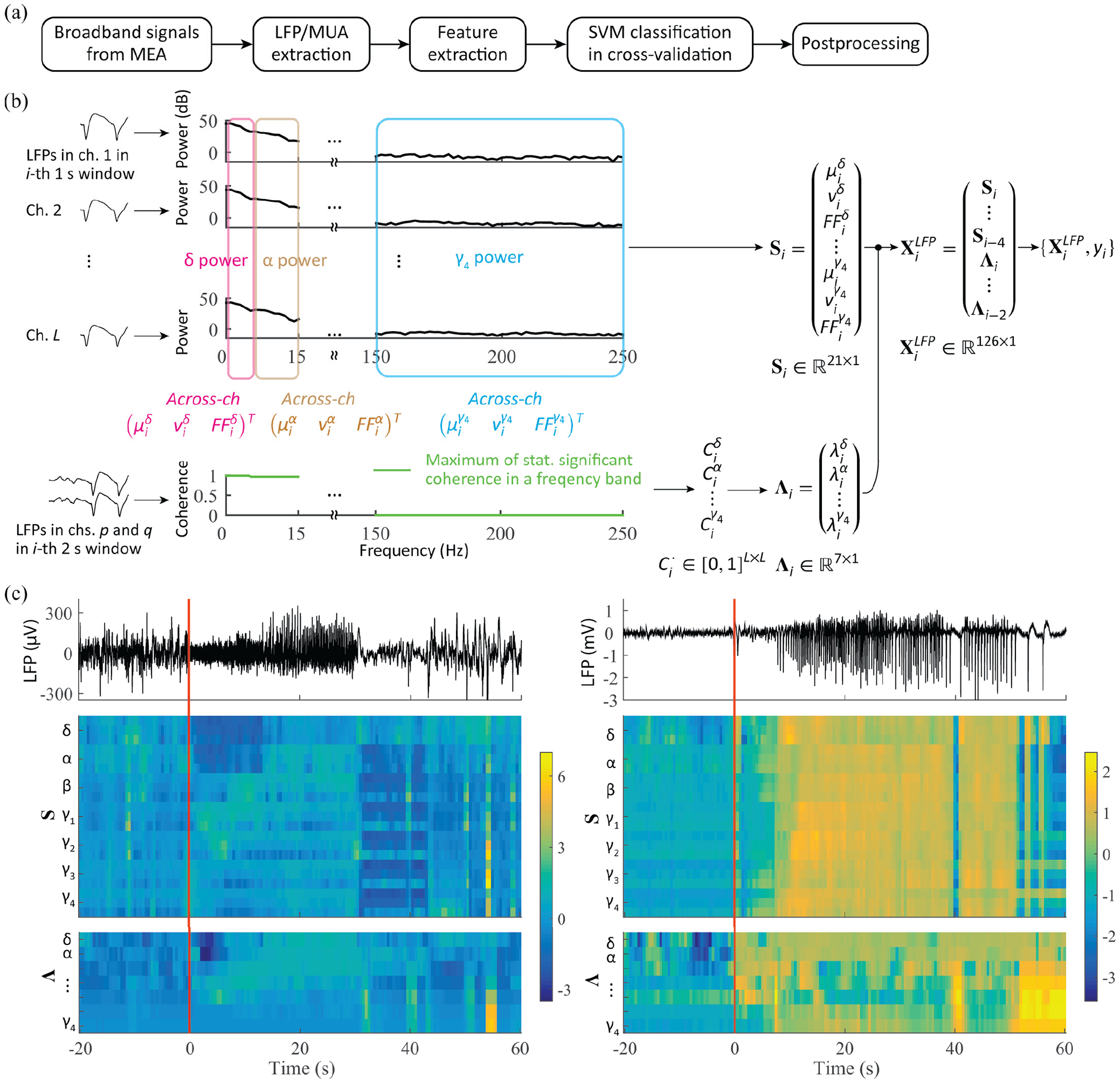
Early seizure detection framework and feature extraction from LFP signals. (a) Framework outline. (b) Feature extraction from LFP: for a given 1 s time window i, the across-channel mean, variance, and Fano factor of spectral power in each of seven bands are computed (S_i), together with the leading eigenvalues (Λ_i) of the matrices of pairwise coherence between LFP channels. The L by L symmetric coherence matrices are computed for each of the seven band, and their entries consist of the maximum values of statistically significant coherence in a given band for each channel pair. (c) Examples of LFP feature over a seizure event: LFP traces in a single channel and their corresponding two feature subsets S and Λ (z-scored) for a gamma-band seizure in P1 (left panel) and for a SWC seizure in P4 (right). Local seizure onset at time 0.

Fig. 3.

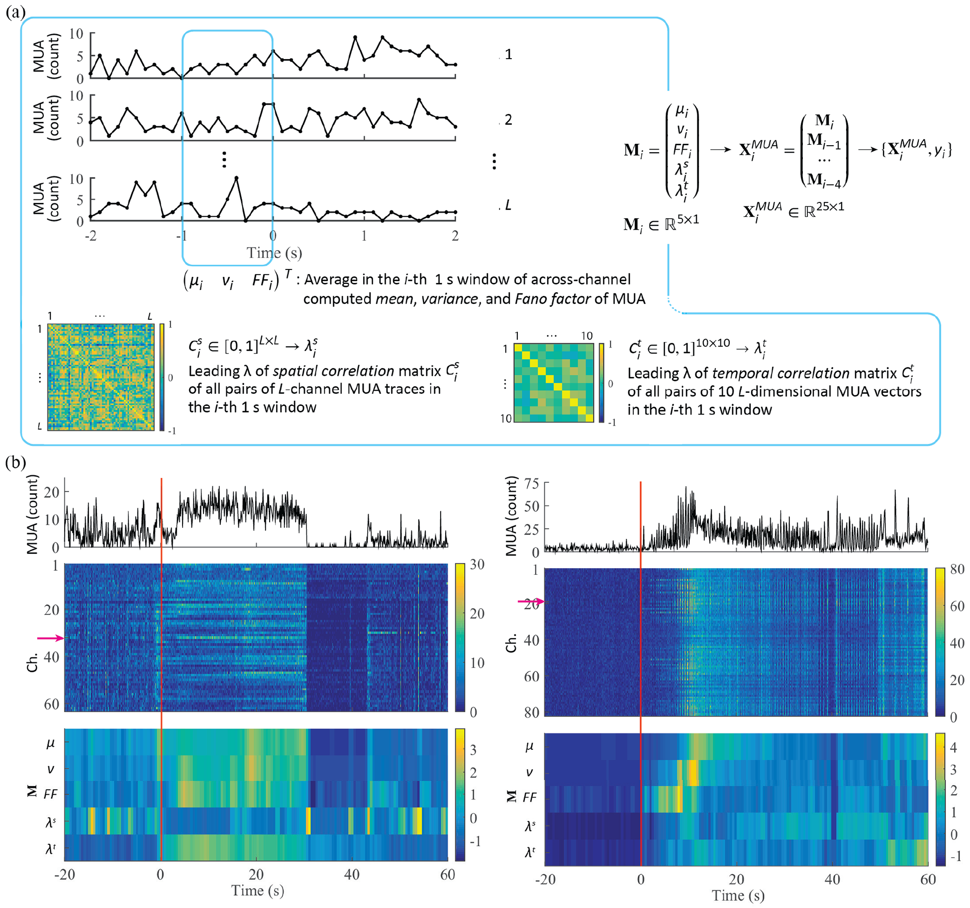
Feature extraction from MUA. (a) Low-dimensional MUA features consist of the mean, variance, Fano factor of MUA computed across all channels in a given 1 s time window, together with the leading eigenvalue of two different pairwise correlation matrices. In the first case, the leading eigenvalue is calculated using the correlation matrix from all pairs of L-channel MUA traces (spatial correlation). In the second case, the leading eigenvalue is computed from the correlation matrix based on all pairs of 10 L-dimensional MUA vectors in the same 1 s time window (temporal correlation). (b) Examples of ld-MUA feature over a seizure event: MUA traces in 0.1 s time bins in a single channel, corresponding MUA traces in all channels (z-scored; the red arrow indicates the channel for the MUA traces in the above panel.), and ld-MUA features (z-scored) for a gamma-band seizure in P1 (left panel) and a SWC seizure in P4 (right).

D. Feature extraction from local field potentials and multiunit activity

LFP features included (1) features based on statistical summaries computed on spectral power in seven frequency bands for each MEA channel, and (2) features based on the channel-pairwise spectral coherence matrix for each of the seven bands (see Fig. 2(b)). Spectra were computed via the multitaper approach (e.g. [19]; The full bandwidth parameter was set to 2 Hz). The seven frequency bands used for the above two feature types consisted of (δ) 0.3–5 Hz, (α) 5–15 Hz, (β) 15–30 Hz, (γ₁) 30–60 Hz, (γ₂) 60–100Hz, (γ₃) 100–150 Hz, and (γ₄) 150–250 Hz. We excluded 60 Hz (line noise) and its harmonics. Spectral power (in dB) in each of the frequency bands was computed from 1 s time windows with 0.5 s step. Then, for each frequency band, statistical summaries across the L recording channels, including the mean, variance, and the Fano factor of the spectral power, were calculated [9]. The leading eigenvalue of the pairwise L × L coherence matrices computed for each of the seven bands was also used as a feature. Spectral pairwise coherences were computed from 2 s time window with 0.5 s steps. For each frequency in a given frequency band, pairwise coherence values that were not statistically significant were set to zero (p-value < 0.01) [17], [20]. A single pairwise coherence value was obtained for each frequency band, which consisted of the maximum coherence value across the frequencies in the given band, and then the leading eigenvalue was computed from the resulting (symmetric) coherence matrix (Fig. 2(b)). The above power- and spatial coherence-related features were concatenated to include previous values over the past three seconds [21]: five causal consecutive sets of the statistical summaries (mean, variance and Fano factor for each band) and three causal consecutive sets of coherence matrix eigenvalues for each band. We note that the leading eigenvalue of the coherence matrix for a given frequency band relates to the amount of spatial coherence in that band (e.g. [19]).

We defined and examined two types of MUA-based features. The first consisted of low-dimensional representations (ld-MUA), including statistical summaries of MUA counts across channels and representative values of correlation matrices of MUA counts (see Fig. 3(a)). These summaries included 1 s time-averages of the mean, variance, and Fano factor of MUA counts, computed across channels. They also included the leading eigenvalues of the spatial and the temporal correlation matrices for MUA counts, computed in 1 s windows. For L channels, an L × L spatial correlation matrix computed in a 1 s window i, $C_i^s$, consisted of the Spearman’s correlation coefficients between all pairs of MUA channels (MUA counts in 0.1 s time bins for each channel spanned 10 time bins in the 1 s window i). Another 10 × 10 matrix in the same window i, henceforth referred to as the temporal correlation matrix, $C_i^t$, consisted of Spearman’s correlation coefficients between all channel pairs. In this case, each 1 s time-window was segmented into 0.1 s time bins, generating a 10-dimensional count vector. The leading eigenvalues were then computed from each of the resulting spatial and temporal correlation matrix, $C_i^s$ and $C_i^t$. In addition to the ld-MUA features, we also defined and examined high-dimensional MUA features (hd-MUA), which included both the corresponding ld-MUA features and the total MUA counts in 1 s time windows for each of the L channels. Similar to the case of LFP features, a 3 s temporal concatenation spanning the past three seconds was applied to the ld-MUA (5 × 5 dimension) and hd-MUA (5 × 5 + 5 × L) features.

As a final note, we emphasize that there is no a priori requirement in our application that different features be computed with time windows of the same length. As described above, we used two different time windows to compute the features: a 1 s time window for features related to LFP power spectra and MUA, and a 2 s window for features related to LFP spectral pairwise coherence. The reason for the latter is that coherence cannot be computed directly from single realizations, requiring averaging. When using single realizations and multitaper estimation, this averaging can be performed over the multiple tapers. The choice of a 2 s window allowed us to average over more tapers than in the case of a 1 s window, providing a more robust coherence estimate in these data. This was not an issue for the features related to LFP power spectra and MUA and thus we chose a shorter 1 s time window, which at least in principle allows for a finer temporal resolution.

E. SVM Scoring Function Values, Postprocessing, and Classification under Cross-Validation.

All input features to support vector machines (SVMs) were z-score standardized: mean and standard deviations were computed only on training data and then used for z-scoring both the training and test data. To address the issue of highly imbalanced condition between ictal and interictal samples, i.e. far fewer ictal samples than interictal, we used cost-sensitive SVMs [22]–[24]. The cost-sensitive factor was set as the ratio between the number of ictal and interictal samples in the training data [25]. We used the radial basis function (RBF) kernel.

For in-sample optimization and out-of-sample testing, we used the double cross-validation scheme [8], [26]. Specifically, given n-seizures and k-hour interictal recordings (k does not need be an integer) from each participant, we trained SVMs on data containing (n-1) seizures and k/n × (n-1) hours of interictal data via a five-fold cross-validation on these data. The SVM cost parameter C and RBF kernel parameter Ȗ were obtained via a grid search; a pair of C and Ȗ parameters were determined as those that produced the highest F-measure, a harmonic mean of the precision and recall in binary classification evaluation [30]. With this best pair, an SVM model was then trained on all the training data, and tested on out-of-sample test data that contained the one left-out seizure and k/n h interictal recordings. For a dataset containing n seizures, this training-testing process was then repeated n times, leaving one seizure out at a time.

The smoothing of SVM scoring function values can reduce the number of false alarms. As a postprocessing step, we applied the Kalman filter to the SVM scoring function (e.g. [8], sup info). We chose a ratio of 2⁻¹⁰ between the process and observation noise variances. This Kalman filtering step reduced isolated false positives (FPs) at the cost of some minor increase in detection latency. In addition, we applied a persistence period of two min refractory time [31]. Once the Kalman-filtered SVM scoring function values crossed the decision threshold, i.e. an alarm was triggered for seizure detection, the alarm state persisted for at least the refractory time. The persistence improved FP per hour rate by ignoring multiple subsequent FPs after the first alarm but at the expense of FP period extension. Examples of SVM scoring functions, Kalman filtering and state persistence are shown and discussed later in Figure 6.

Fig. 6.

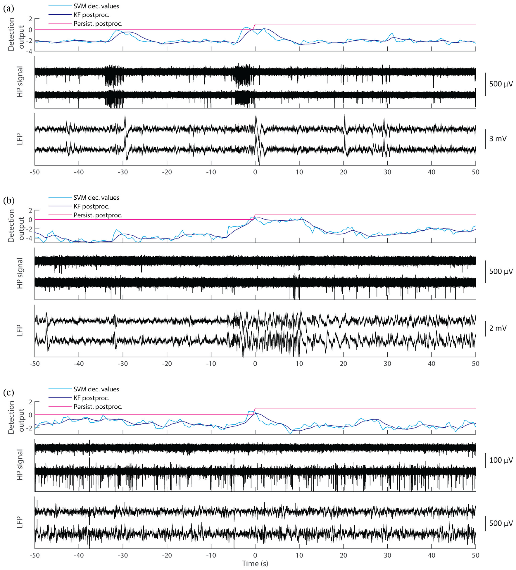
False positive (FP) analysis. Out of a total of 25 FPs (Table I), 14 corresponded to epileptiform discharge activity (7/25, see panel (a)) or subclinical events (7/25, see panel (b)). The other 11 FPs were identified as algorithm failure or recording artifacts, with 3 of those occurring during the 10-min preictal periods.

F. Feature Importance

To assess which features contribute more to the detection performance, we quantified feature importance using extreme gradient boosting (XGBoost) classification. XGBoost is a highly efficient and accurate machine learning algorithm based on scalable regression tree framework using gradient boosting [32]. (The software package, coded in Python 3.6, is freely available at https://xgboost.readthedocs.io/en/latest/). As a tree structure, the XGBoost classification inherently provides a way to rank the importance of each feature to the classification performance.

We first performed an XGBoost-classifier model selection via a grid-search of (in five-fold cross-validation) of two hyperparameters consisting of the maximum depth of a tree and the minimum sum of instance weights required in a child. Also, to handle the imbalanced condition of ictal and interictal samples, ictal samples were weighted by the ratio of the number of ictal and interictal samples. Then, using a determined well-fit model, feature importance scores were calculated as described in [32].

G. Assessment of Ictal and Interictal Class Separability, and latency/accuracy trade-offs

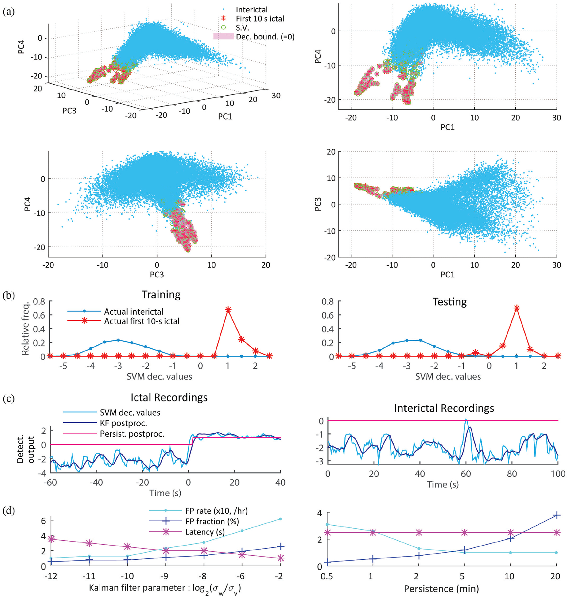
Beyond the assessment of MUA defined as counts of threshold crossing of highpass-filtered MEA potentials in 0.1 s time bins, we also examined the effect of different MUA thresholds on ictal and non-ictal class separability (See Fig. 4(c)). We considered five different thresholds for MUA count features, obtained by varying threshold levels from −5 × SD to −1 × SD. In addition, we considered two other MUA definitions obtained by using continuous valued signals (not counts). The first one was defined as the root-mean-square value of clipped (± 2 SD) highpass-filtered MEA potentials in 0.1 s time windows [27], and the other was as integration in 0.1 s windows of absolute values of highpass-filtered MEA potentials, followed by the logarithm transformation [28].

Fig. 4.

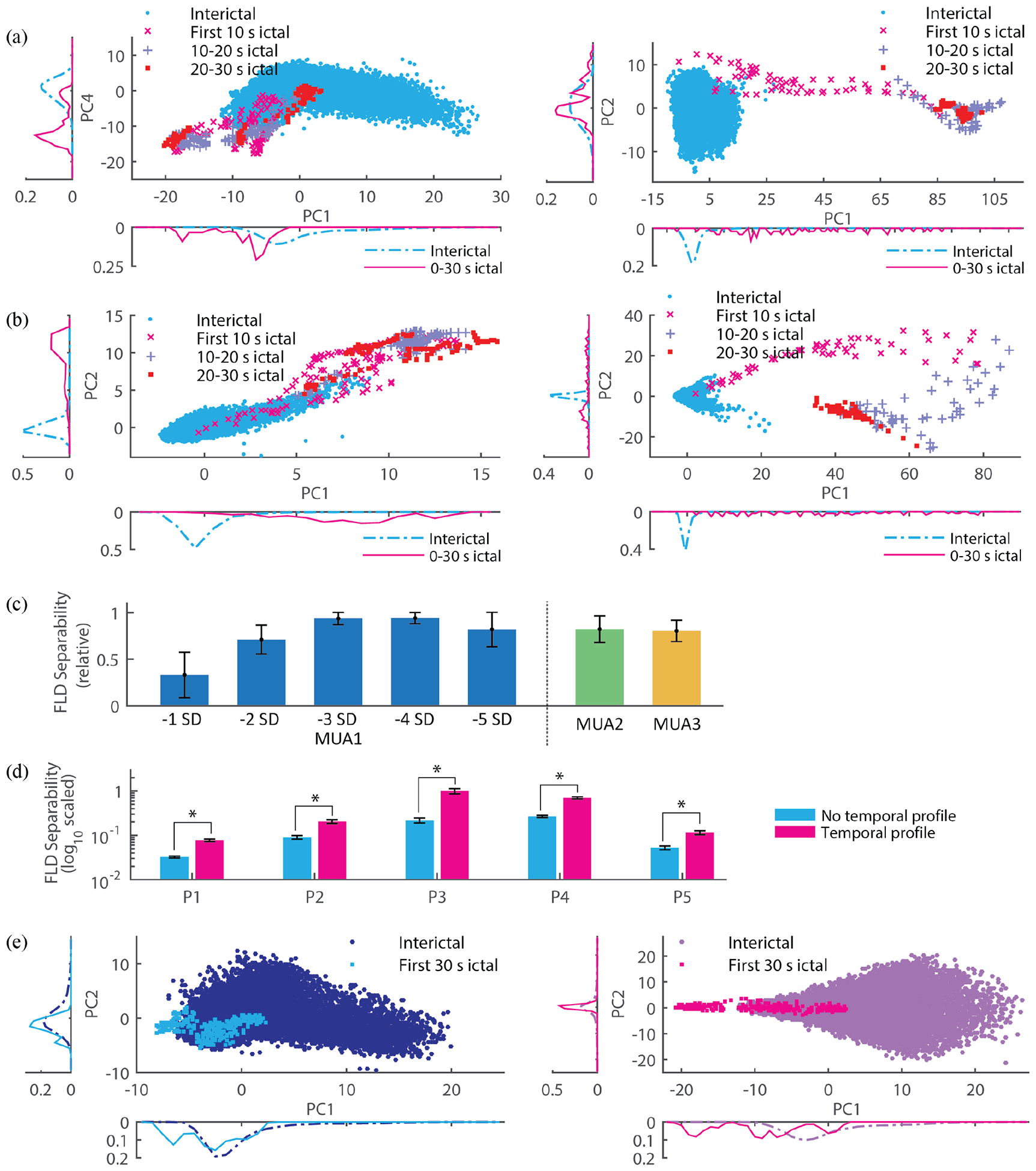
(a) Projection of LFP features into a 2D space obtained via principle component analysis (PCA; PC 1, 2, … refer to the first, second, and so forth components) for participant P1 (left panel) and P4 (right). Each point in the projection corresponds to a 1 s time window during interictal periods or during initial stages of the seizures (e.g. the first 10 s, and so on). The side plots refer to the relative frequency histogram on a corresponding PC. (b) Same conventions as in 2D but with ld-MUA features. (c) Dependence of class separability (ictal vs interictal) on different definitions of MUA. Fisher linear discriminant (FLD) analysis was used to quantify class separability between ictal and interictal ld-MUA features. MUA1 corresponds to ld-MUA feature, i.e. across-channel averaged counts and so on, generated based on MUA counts. We note that these MUA counts were defined with respect to various thresholds, each specified in terms of standard deviations (SD). MUA2 and MUA3 correspond to continuous valued signals (not counts): root-mean-square values of clipped high-pass filtered signals as specified in [27], and integration of log-scaled high-pass filtered signals as specified in [28], respectively. The bar indicates the mean across all the participants (the separability maximum across the different MUA definitions in a participant was set as one to minimize the effect of the participants’ variability), and the error bar indicates one SD. Among all of the MUA definitions, the largest separability was achieved by MUA counts with respect to a −3 SD threshold. (d) The use of temporal profile, i.e. a feature vector comprises values from the current and past time windows (Materials and Methods), provided significantly larger separability of ictal and non-ictal classes (p < 0.01 by random permutation test in [29] than the alternative of using features computed only from the current time window (no temporal profile). The bar indicates the mean in a participant across FLD separability measures through resampling and rebalancing, and the error bar indicates one SD. (e) An example from P1 illustrating the increase in separability by temporal profile (left panel without temporal profile and right panel with it). The visual comparison between the left and right panels clearly shows a significant increase of class separability. The 2D projections are based on the two leading principal components, PC 1 and PC 2 (same conventions as in Fig. 4(a)).

We also examined the effect of concatenating features from past time windows (temporal profiling) by comparing class separability (ictal vs non-ictal) with and without time window concatenation. We quantified ictal and interictal class separability by using the Fisher Linear Discriminant (FLD) [33], [34], and data rebalancing [35]. We note that our use of the Fisher linear discriminant, as opposed to typical linear discriminant analysis (LDA), made no homoscedasticity or normality assumptions. First, in the FLD formulation each class has its own covariance. Second, instead of assuming normality in the statistical comparison of FLD values (Fig. 4(d)), we used a resampling/random permutation test [29] to estimate the distribution under the null hypothesis. In addition, we assessed the trade-off between detection latency and detection performance in terms of false positive rates and fractions. We analyzed various combinations of postprocessing parameters and corresponding event-wise detection performance. The parameters included the ratio of the state and observation noise variances for the Kalman filtering and refractory time, i.e. the duration of the persistence period. We varied the variances’ ratio from 2⁻¹² to 2⁻² (with steps of power of 2) with a fixed refractory time of 2 minutes in the persistence postprocessing. We varied the persistence period from 0.5 min to 20 min with a fixed Kalman filtering parameter of 2⁻¹⁰.

III. Results

We assessed the performance of the participant-specific framework for early seizure detection on MEA recordings that included 17 seizures and 39.0 h preictal and interictal periods from five participants. As stated earlier (Materials and Methods), we formulate the seizure detection as a two-class classification problem: ictal vs interictal/non-ictal classes. Ictal samples correspond to samples obtained during the seizure. For fitting of SVM classifiers to training data, non-ictal samples corresponded to interictal recordings. (Except for the SVM hyperparameters, which were set to the same values across participants, SVM classifiers were participant-specific, i.e. trained on each participant’s dataset separately; all other parameters related to Kalman filter postprocessing, etc., were set to the same values across participants.) For classification assessment on test data, non-ictal samples contained both interictal and preictal samples. To assess detection performance in cross-validation, we calculated event-wise sensitivity, detection latency, false positive (FP) rate per hour, and the fraction of FPs during preictal and interictal periods (Materials and Methods). Event-wise sensitivity represents the proportion of detected seizures with respect to the number of actual seizures. Detection latency quantifies how early seizures can be detected with respect to gold standard detection onsets, retrospectively determined in MEA or iEEG recordings by an expert encephalographer (S.S.C.). FP rate and FP fraction in preictal and interictal periods quantify how often and how long false alarms are generated by the framework, respectively. In addition, we assessed the area under the Receiver Operating Characteristic (ROC) curve (AUC) as done in previous seizure detection studies, e.g. [36].

A. Localized intracortical MEA recordings away from seizure onset areas allow for early seizure detection

Table I summarizes detection results across all the five participants and Fig. 5 illustrates individual results from each of the participants. Both were categorized in terms of five signal/features types, i.e. features based on LFP, low-dimensional MUA (ld-MUA), high-dimensional MUA (hd-MUA), combined LFP and ld-MUA (LFP + ld-MUA), and combined LFP and hd-MUA (LFP + hd-MUA, see Materials and Methods for details). In the following, based on Fig. 4(c) (see also section G), we set the MUA threshold to – 3 SD.

TABLE I.

Detection performance organized by feature types across all the participants’ recordings: sensitivity (# detected seizures/ # actual seizures), detection latency (median, mean [minimum, maximum]), FP rate per hour (# FPs (# FPs in preictal period) / non-ictal recording Hours), and FP fraction with respect to non-ictal periods.

	Signal/feature type
	LFP	ld-MUA	hd-MUA	LFP + ld-MUA	LFP + hd-MUA
Sensitivity (%)	100% (17/17)	100% (17/17)	100% (17/17)	100% (17/17)	100% (17/17)
Latency (s)	2.5,−7.6 [−183.0, 10.0]	3.5,−6.4 [−104.0, 12.0]	2.5,4.5 [0.0, 14.5]	2.5,−2.1 [−79.5,8.0]	2.5, 3.5 [−3.0, 13.0]
FP rate (/h)	0.13/h (5 (l)/39.0 h)	0.15/h (6 (0)/39.0 h)	0.08/h (3 (0)/39.0 h)	0.13/h (5 (l)/39.0 h)	0.13/h (5 (l)/39.0 h)
FP fraction (%)	0.45%	0.85%	0.26%	0.77%	0.45%

Fig. 5.

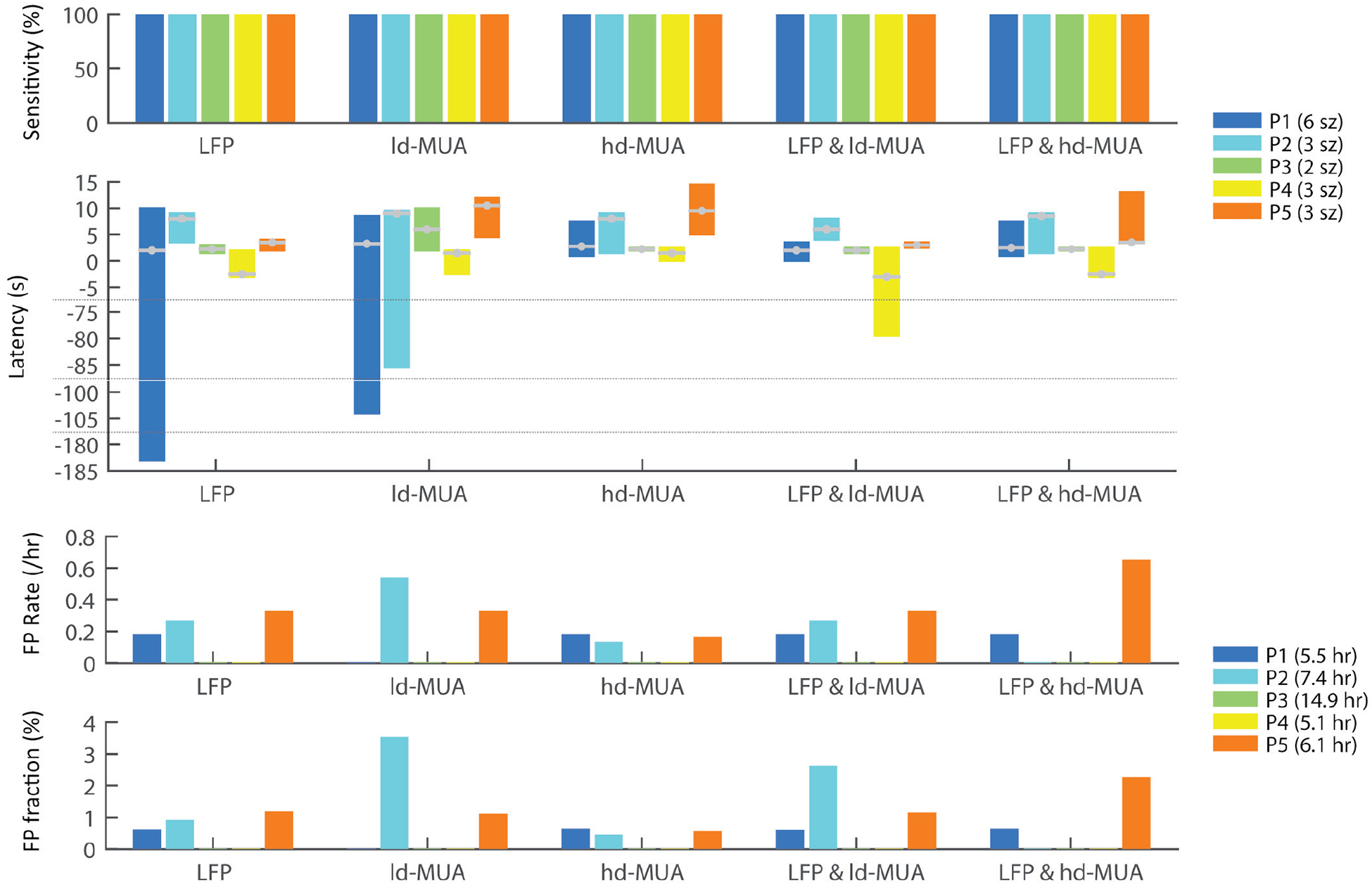
Detection performance in individual participants for different signal/feature types: sensitivity, detection latency, false positive rate per hour, and false positive fraction in non-ictal recordings. P1-P5 indicate the individual participants; “sz” and “h” denote the seizure number and the number of non-ictal hours in the test datasets. In the latency plot, the grey lines with a filled circle in each bar represent the median latency in the corresponding participants.

Detection with 100% sensitivity (all 17 seizures were detected) was achieved with any of the individual or combined feature types. Detection with LFP features resulted in median latency of 2.5 s and mean of −7.6 s (negative latency means that detection alarms were triggered before the seizure onsets and persisted beyond seizure onset; see Materials and Methods), and four and one false alarms in interictal and preictal periods, respectively, adding up to a total of 10.5 min false alarm duration in the 39.0 h non-ictal recordings, with 0.13 FP per hour and 0.45 % of the non-ictal recordings. Detection based on ld-MUA features resulted in slightly increased median latency of 3.5 s (mean of −6.4 s). Six false alarms were triggered during interictal periods (0.15 FP per h) with a total false alarm duration of 19.9 min (0.85 %).

Detection with hd-MUA features showed similar median latency of 2.5 s to that with LFP or ld-MUA features, but increased mean latency of 4.5 s due to no true positive (TP) alarms triggered during the immediately preceding preictal periods that continued over the seizure onsets in P1 and P2, as seen above. The use of this feature resulted in the smallest number (three false alarms, 0.08 per h) and shortest duration (6.1 min, 0.26 %) of false alarms among the five features. From the perspective of binary classification of ictal from non-ictal samples without consideration of detection latency, hd-MUA features showed the best performance with the smallest FP number and FP fraction.

B. LFP + ld-MUA features produce the best performance with respect to detection latency and the AUC analysis.

The use of combined LFP and ld-MUA features resulted in median detection latency of 2.5 s and mean latency of −2.1 s, with one very early true positive (TP) alarm (−79.5 s) in P4. Considering that all of the very early TP alarms that occurred with individual LFP features, ld-MUA features, and combined LFP + ld-MUA features turned out to be initiated with no specific noticeable events but as algorithm failures (discussed later in detail), LFP + ld-MUA features actually generated the quickest detection latency with its least variance: median latency of 2.5 s, mean of 2.7 s, and the smallest of −3 s and the largest of 8 s. LFP + ld-MUA features generated four FPs in interictal periods and one FP in preictal periods, summing up to 18.0 min FP duration in non-ictal periods (0.13 FP per h and 0.77 % FP duration). The combination of LFP and hd-MUA features produced similar detection latency values to that obtained with hd-MUA features, with median of 2.5 s and mean of 3.5 s. It resulted in five FPs in non-ictal periods with a total duration of 10.5 min (0.13 FP per h and 0.45 % FP duration), similarly to the case of the use of LFP features only. We note that, in addition to the above results based on individual or combined features, seizure detection in P3 and P4 showed no FPs with any of the feature types.

The above results were also corroborated with the AUC analysis results shown in Table II. Detection performance was assessed by averaging two AUC values computed using standardized Kalman-filtered SVM scoring function values in ictal versus non-ictal periods (AUC_sz) and in early seizure (first 30-s) versus non-ictal periods (AUC_early) [36]. We calculated those three AUC values per feature. The highest detection performance, obtained by combining LFP + ld-MUA features, corresponded to AUC = 0.97; (An AUC = 0.5 corresponds to chance level, and an AUC = 1 corresponds to perfect detection).

TABLE II.

Detection performance organized by feature types across all the participants’ recordings: area under the ROC curves.

	Signal/feature type
	LFP	ld-MUA	hd- MUA	LFP + ld-MUA	LFP + hd-MUA
AUCsz	0.9293	0.9296	0.9598	0.9779	0.9595
AUCearly	0.9577	0.9568	0.9726	0.9626	0.9668
Performance	0.9435	0.9432	0.9662	0.9702	0.9632

C. Feature importance

Quantification of importance of the features used in the detection analysis may help understand how relevant LFP and MUA-based features contributed to the detection performance. Using the combined LFP-ld-MUA features, which produced the highest detection performance in the AUC analysis, we assessed feature importance based on the feature ranking obtained via XGBoost classifiers (see Materials and Methods). Table III shows the top 10 ranked features for each of the participants, and Supplementary Fig. 3 presents this analysis in more detail for each of the participants.

Table III.

Feature importance. The LFP coherence-based features are shown in bold and the MUA-based features are underlined. The number in the parenthesis represents the relative importance of the corresponding feature according to XGBoost classifiers, with most important features to the left. (See Figs. 2–3 and Material and Methods for the adopted symbols.)

ID	Feature importance
P1	μδ (0.061)	λγ3 (0.056)	μγ4 (0.055)	λγ1 (0.053)	FFβ (0.052)	FFγ2 (0.051)	λt (0.050)	λβ (0.047)	FFγ1 (0.039)	λγ2 (0.039)
P2	λγ4 (0.047)	λγ2 (0.046)	μγ2 (0.045)	λδ (0.041)	μ (0.040)	μβ (0.040)	λγ1 (0.040)	FFγ3 (0.039)	FFα (0.038)	FF (0.038)
P3	μ (0.097)	FFα (0.075)	λγ2 (0.072)	v (0.058)	λs (0.057)	λδ (0.054)	μα (0.044)	μβ (0.044)	FFγ3 (0.043)	FFγ1 (0.042)
P4	λγ1 (0.179)	v (0.173)	λα (0.116)	FF (0.114)	λβ (0.089)	μ (0.086)	μα (0.036)	FFγ1 (0.036)	λγ2 (0.034)	vα (0.021)
P5	λδ (0.068)	μ (0.053)	λβ (0.052)	λγ4 (0.047)	FF (0.044)	vα (0.044)	FFδ (0.042)	μγ4 (0.041)	λγ1 (0.039)	λγ3 (0.038)
Median	μ (0.053)	λβ (0.047)	λδ (0.041)	λγ1 (0.040)	μγ4 (0.039)	λγ2 (0.039)	FF (0.038)	FFγ1 (0.036)	λγ3 (0.035)	μα (0.032)
Mean	λγ1 (0.063)	μ (0.060)	v (0.057)	λβ (0.051)	FF (0.047)	λγ2 (0.045)	λα (0.045)	λδ (0.039)	FFγ1 (0.036)	μα (0.034)

Overall, LFP coherence-based and MUA count-based features were determined as top ranked features. Interestingly, the feature ranking differed between P1 (seizures characterized by gamma oscillations) and P2–5 (seizure characterized by spike-wave complexes). Specifically, the top features for P1 corresponded to LFP spectral power-based features, while for P2–5 the top features tended to related to LFP coherence-based and MUA count-based features.

D. Seizure detection performance based on iEEG determined seizure onsets

For completeness of the detection analysis in MEA recordings, we also investigated seizure detection based on MEA recordings with respect to gold standard seizure onsets determined in iEEG recordings. Supplementary Tables I and II show detection results from MEA recordings with respect to iEEG-defined onsets in the first four participants and in P3, respectively. The results were tabulated separately, because the two recorded seizures in P3 remained very localized for tens of seconds in one to two iEEG sites before a sudden spread across the remaining iEEG and MEA sites (Material and Methods). iEEG-identified onsets were 1.8 s earlier in average than seizure onsets identified on the MEA recordings in P1, P2, P4, and P5, and 90.6 s earlier in P3 (Materials and Methods).

We note that Supplementary Table I shows results from 14 seizures, because one seizure in P5 was not identifiable in iEEG recordings due to a failure in the iEEG recording system. Results inSupplementary Table I are very similar to results shown in Table I: 100 % sensitivity (14/14) with any of the five features and 2.5 s to 3.8 s median detection latency with some increase in FP rate and fraction. However, analysis of Supplementary Table II based on participant P3 data shows contrasting results. Seizures in P3 with respect to iEEG-identified onsets were almost not detectable. Furthermore, the only detected seizure, based on ld-MUA features, can be considered incorrect, considering the very high FP fraction.

E. Most technical false alarms originated from epileptiform activity or subclinical events

We examined in detail all of the recording segments where false alarms occurred, a total of 24 FPs. We found that recordings corresponding to FPs consisted of either epilepsy-related events (14/24, 58.3 %), such as epileptiform discharge activity (e.g. bursts of interictal discharges) and subclinical events, or algorithm failure (10/24, 41.7 %). Out of the 14 epilepsy-related events, half occurred with epileptiform discharges in P2 (see Fig. 6(a)), and the other half occurred during subclinical events in P5 (see Fig. 6(b)). Ten FPs occurred without any obvious abnormal events in P1, P2, and P5, and thus were counted as algorithm failure (see Fig. 6(c)). Three of the ten FPs due to algorithm failure occurred during preictal periods (two in P1 and one in P5). If an alarm was triggered during a preictal period but did not persist over the gold standard onset, it was counted as a FP. P3 and P4 showed no FPs.

In a feature-wise based FP analysis, we examined whether a FP event resulted from epileptiform discharges, subclinical events or algorithm failure: five FPs occurred with LFP features (two due to epileptiform discharge activities, two due to subclinical events, and one due to algorithm failure); six FPs with ld-MUA features (three, one, and two, respectively); three FPs with hd-MUA features (none, one, and two, respectively); five FPs with LFP + ld-MUA features (two, one, and two, respectively); and five FPs with LFP + hd-MUA features (none, two, and three, respectively). Other than the one algorithm-failure FP with LFP features during a preictal period, all the FPs generated with LFP features were related to epileptiform abnormal activity. We note that hd-MUA features and LFP + hd-MUA features generated no FPs related to epileptiform discharges.

We also investigated preictal recordings with TP alarms that occurred earlier than the gold standard onset, suggesting prediction of ictal events. As stated above, if an alarm was triggered ahead of the seizure onset and persisted continuously at least until the actual seizure onset time, we counted it as a TP. A total of ten early TP alarms occurred, with two in P1, one in P2, and seven in P4. Six out of the seven early TPs in P4 occurred right before the seizure onsets (2.8 s in average ahead of onset). These early TPs occurred during epileptiform abnormal activity observed in the MEA recordings before the gold standard onsets. In contrast, MEA recordings where the four early FPs occurred showed no obvious abnormal activity.

F. Effect of imbalanced datasets and postprocessing on SVM early-seizure detection

We used cost-sensitive nonlinear SVM classification for the early seizure detection. Fig. 7(a) shows our classification results using cost-sensitive nonlinear SVMs on lower-dimensional projections of the feature space. Nonlinear SVMs can suffer from data overfitting [26]. Similar distributions of SVM scoring function values for both the training and testing cases in Fig. 7(b) indicate that overfitting was not an important issue in our classification models. Fig. 7(c) shows the effect of postprocessing of SVM scoring function values by Kalman filtering. Although Kalman filtering slightly increased detection latency due to “dampening” of scoring function values, it improved detection performance by reducing the number of FPs by smoothing out sporadic large positive values.

Fig. 7.

Classification using cost-sensitive nonlinear SVMs and Kalman filter postprocessing. (a) An illustrative example from participant P1 shows the 2D and 3D projections of non-ictal and ictal samples on the first, second, and fourth principal components, together with the support vectors and the SVM decision boundary. Cost-sensitive nonlinear SVMs managed well the highly imbalanced data, i.e. only a few ictal samples out of abundantly many non-ictal samples were classified as ictal. (b) Relative frequency plots of SVM scoring function values in training and testing data from P1. Positive and negative scoring function values correspond to samples (1 s time windows) classified as ictal and non-ictal samples, respectively. The similar distributions in both training and testing indicates that the SVM classifier was not strongly affected by the common overfitting problem in imbalanced datasets [37]. (c) Postprocessing of SVM scoring function values: Kalman filtering and persistence [31]. Two examples of postprocessing are shown during ictal recordings (left panel) and interictal recordings (right). Samples with positive postprocessed scoring function values result in a seizure alarm. Although the postprocessing procedure may worsen slightly detection latency (1 s in the left panel example), it improves overall the detection performance by lowering the number of false alarms. That is achieved by smoothing incorrect and sporadic SVM values during non-ictal periods (e.g. the event around 60 s in the right panel). (d) Trade-off analysis between detection latency and detection performance (false positive rate and fraction) as a function of the Kalman filtering parameter (left panel) and as a function of the duration of the adopted persistence postprocessing (right). As the ratio of the state and observation noise variances (σ_w /σ_v) in the Kalman filtering increased from 2⁻¹² to 2⁻², the average FP rate deteriorated from 0.10 /h to 0.62 /h, while the median latency across all the participants’ recordings enhanced from 3.5 s to 1 s. On the other hand, the increase in the refractory time (persistence) did not affect detection latency but worsened FP detection performance (FPs occurred less frequently, but once a FP occurred it lasted longer).

G. Effect of different MUA threshold and definitions and different temporal profiling on the separability of ictal and non-ictal samples

We examined the effect of several different MUA threshold and definitions (Fig. 4(c); Methods and Material) and temporal profiling (Fig. 4(d) and (e)) on ictal and non-ictal class separability. First, we examined class separability based on the first 30-s ictal and non-ictal ld-MUA features under several MUA definitions, including MUA counts (MUA1) with several different threshold levels, MUA enveloped obtained as root-mean-square values of MUA (MUA2), and integration of log-scaled absolute values of high-pass filtered MEA potentials (MUA3). Relative separability (maximum separability in a participant across all the definitions’ averages to one) was used to reduce variability across participants. Fig. 4(c) shows that the use of MUA1 (with thresholds set to −3 SD) resulted in the highest class separability based on the FLD measure. (See Supplementary Fig. 4 for individual participants’ results.)

Second, we analyzed the effect of temporal profiling (time window concatenation) in features using the same FLD analysis (see Materials and Methods). We compared class separability based on the first 20-s ictal and non-ictal LFP + ld-MUA features, with and without temporal profiling. Fig. 4(d) shows that the use of features with temporal profiling resulted in significantly larger class separability (p < 0.01; random permutation test). We note that the effect of concatenating time windows over shorter or longer periods than adopted here on detection performance remains a problem for future examination.

H. Effect of postprocessing parameters on detection performance and detection latency

When a seizure detection algorithm shows a certain degree of detection accuracy and latency, there might be a trade-off between the two. In other words, a parameter adjustment toward better latency may lead to poorer detection performance, and vice-versa. In particular, we quantified this trade-off by varying parameters related to the postprocessing of the SVM scoring functions, specifically the ratio the state and observation noise variances in the Kalman filtering and the refractory time for the persistence period.

As the ratio parameter between process and observation noises increased from 2⁻¹² to 2⁻² in the Kalman filtering postprocessing, i.e., the smoothing of SVM scoring functions decreased, resulting in an increase in FP rates and fractions (Fig. 7d, left). On the other hand, as the refractory time in the persistence postprocessing was extended from 0.5 s to 20 s, the median detection latency stayed the same at 2.5 s, and FPs occurred less frequently, but with much longer periods (Fig. 7d right). Regardless the variations in the two parameters for the postprocessing as described above, sensitivity remained at 100 % in all the cases.

IV. Discussion

Our findings demonstrate that early seizure detection can be successfully achieved using intracortical signals recorded via MEAs placed in small (4 × 4 mm²) neocortical patches ~ 2 – 5 cm away from identified seizure onset areas. To our knowledge, this is the first study to investigate the use of MEA signals for detection of human epileptic seizures. In addition to showing that human epileptic seizures can be reliably detected with features from LFPs and/or MUA recorded in MEAs, we demonstrated that combination of those features can provide synergistic positive effects on the detection performance. The combined LFP + ld-MUA features showed not only the earliest detection latency but also the best AUC-based detection performance. The AUC-based performance was comparable to those achieved by the top ranked approaches in a Kaggle competition for seizure detection based on large-scale subdural ECoG recordings [36]. (Nevertheless, we also note that in our application, we had access to the relative time of each sample, while that was not the case in the Kaggle competition; that could have potentially contributed to the performance.) It remains an open issue how the framework and algorithms proposed here compare to several other approaches, e.g. [38] and in the Kaggle competition [36], which have been applied to scalp or intracranial (but not intracortical) EEG signals. Our findings indicate that the use of intracortical signals may open new possibilities for quick and reliable detection of human epileptic seizures.

Prior studies from a pilot clinical trial aiming at restoring movement and communication for people with paralysis have shown that MEAs can be used chronically for many years [8], [9]. Ongoing development of MEA devices is expected to further improve its performance in chronic recordings, making them also a potential recording approach for other neurological disorders such as focal epilepsies.

Given the algorithms used in this study, the use of LFP features resulted in slightly better detection performance than detection based on MUA features. Because the MEAs were placed in neocortical patches distal to the seizure onset areas, one possibility is that non-local inputs from the onset areas drove subthreshold postsynaptic potentials and were captured first in the LFP signal during the initial stage of the seizure, while MUA captured the subsequent recruitment effect on local neuronal spiking activity. We note, nevertheless, that the combination of LFP and MUA features improved performance. In addition, MUA features seem more sensitive to brief epileptiform activity during interictal periods and subclinical seizures, and this was indicated in the analysis of FPs for MUA-based detection during interictal periods. The detection of epileptiform activity during interictal and preictal periods may be important for successful responsive, or closed-loop seizure control systems.

A challenge in seizure detection studies is that datasets are typically highly imbalanced, i.e., ictal samples are extremely rare in comparison to non-ictal ones. To handle the highly imbalanced condition, we used cost-sensitive SVMs, i.e. misclassification of samples in ictal periods was penalized much more than misclassified of non-ictal samples. In this study, we set the cost-sensitive factor to the ratio of the number of samples in the two classes. Classification with over-sampling [39] or under-sampling [22] can be an alternative to cost-sensitive classification.

We used the F-measure for model selection in training in the double cross-validation. The F-measure is often used in machine learning to quantify how well rare samples in a minor group, i.e., ictal samples, are classified [40]. However, the F-measure does not capture the number of true negative samples, i.e., correctly classified samples in interictal periods, and may in some cases be too sensitive to a small number of TP samples. We note that a sample-wise high F-measure does not necessarily imply high event-wise detection rate.

Temporal profiling, i.e. the concatenation of current and preceding features within a given history window for each feature [21], improved the separability between ictal and interictal samples (p-value < 0.01). Here, we chose a history window of 3 s as the length of temporal profiling for computational convenience. It is possible that longer history windows may improve detection performance.

We note that our early detection approach does not provide information about whether a seizure that just started will spread or remain focal, or whether it will manifest as a clinical seizure or not. We have addressed the problem of seizure propagation from a neural dynamics perspective in [41]. The issue remains an important problem for the development of closed-loop seizure control systems. We hope to examine in the future the inclusion of single-neuron spiking activity [17] and compare detection performance based on these intracortical signals to performance based on intracranial EEG signals. Successful seizure detection with short latencies were obtained in this study using recording from MEAs implanted in small neocortical areas distal to the identified seizure onset areas. We expect that further improvement in detection performance is likely to be achieved by implanting MEAs (or similar devices containing microelectrodes, not necessarily planar arrays) in identified seizure onset areas. (This approach would address in particular the cases of focal seizures that remain very localized for a long period before spreading, as seen for the case of participant P3.) The possibility of better targeting identified seizure onset areas with MEA implants, as well as the comparison of MEA vs iEEG signals, remains an open question for future studies.

The current study – like all clinically, relatively time-limited intracranial seizure monitoring – may be confounded in part by the recent craniotomy and changes in anti-epileptic medications. In the context of next-generation closed-loop systems for seizure control, one can envision the identification of seizure onset and epileptogenic areas during the neuro-monitoring period preceding device implantation, the opportunity to constantly refine and improve seizure detection accuracy over extended periods, and the use of microelectrodes on platforms of different shapes and depths to further improve data quality.

V. Conclusion

Our study sheds new light on the use of intracortical neural signals recorded via microelectrode arrays for early detection of focal seizures in people with pharmacologically resistant seizures, in particular the use of multiscale signals including LFPs and MUA. Using a detection framework with nonlinear SVM classification, we analyzed several LFP, MUA and combined LFP-MUA features in the recordings that included 17 seizures and 39.0 h interictal state from five participants with epilepsy. While LFP- and MUA-based features separately allowed 100% sensitivity, their combination improved not only ROC-based measures but also detection latency. Detection performance was comparable to previously reported seizure detection based on larger-scale iEEG recordings. Analysis based on XGBoost classifiers ranked features based on LFP spectral coherence and MUA count as top features for participants with SWC seizures, while features related to LFP power spectra were ranked higher for the participant with seizures characterized by sustained gamma LFP oscillations.

Fig. 1.

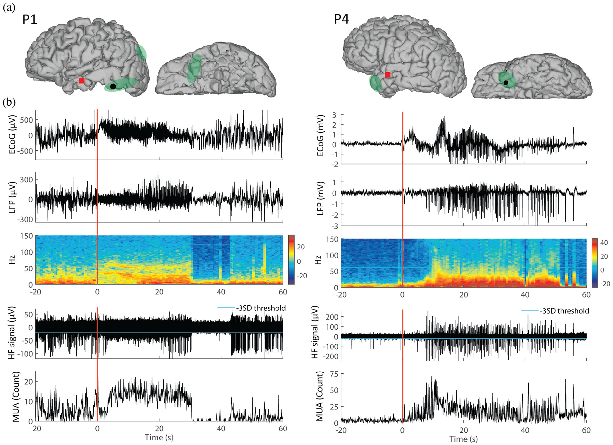
ECoG, LFP, and MUA traces for two different types of epileptic seizures. The left panel is illustrated with a seizure characterized by sustained gamma-band oscillations recorded in P1, and the right panel is with a seizure characterized by spike-and-wave complexes recorded in P4. (a) Locations of the implanted microelectrode array (MEA, red square) and of one subdural ECoG electrode (black dot). Green shaded areas correspond to seizure onset zones as identified by iEEG inspection. (b) The top panel shows ECoG time traces recorded from the electrode shown in (a). The LFPs recorded from one channel in the MEA and the corresponding spectrogram are shown in the two bottom panels, respectively. (c) Highpass-filtered signals (HF signals, > 300 Hz) from the same MEA channel and the corresponding multiunit activity (MUA), defined by the number of HF signals in 0.1 s time bins crossing the threshold (cyan line representing −3 × SD of the MUA). Time 0 refers to local seizure onsets identified in MEA recordings. Corresponding iEEG-identified seizure onsets occurred at −1.17 s and - 0.10 s in the left panel and right panel, respectively. (MRI images in (a) are modified versions from images in Truccolo et al., 2014 [17].)

REFERENCES

- [1].Thurman DJ et al. , “Standards for epidemiologic studies and surveillance of epilepsy,” Epilepsia, vol. 52, no. s7, pp. 2–26, 2011. [DOI] [PubMed] [Google Scholar]
- [2].England MJ, Liverman CT, Schultz AM, and Strawbridge LM, “Epilepsy across the spectrum: Promoting health and understanding.: A summary of the Institute of Medicine report,” Epilepsy Behav, vol. 25, no. 2, pp. 266–276, 2012. [DOI] [PMC free article] [PubMed] [Google Scholar]
- [3].Zaccara G, Franciotta D, and Perucca E, “Idiosyncratic adverse reactions to antiepileptic drugs,” Epilepsia, vol. 48, no. 7, pp. 1223–1244, 2007. [DOI] [PubMed] [Google Scholar]
- [4].Perucca P, Carter J, Vahle V, and Gilliam FG, “Adverse antiepileptic drug effects Toward a clinically and neurobiologically relevant taxonomy,” Neurology, vol. 72, no. 14, pp. 1223–1229, 2009. [DOI] [PMC free article] [PubMed] [Google Scholar]
- [5].Löscher W and Schmidt D, “Modern antiepileptic drug development has failed to deliver: ways out of the current dilemma,” Epilepsia, vol. 52, no. 4, pp. 657–678, 2011. [DOI] [PubMed] [Google Scholar]
- [6].Heck CN et al. , “Two-year seizure reduction in adults with medically intractable partial onset epilepsy treated with responsive neurostimulation: Final results of the RNS System Pivotal trial,” Epilepsia, vol. 55, no. 3, pp. 432–441, 2014. [DOI] [PMC free article] [PubMed] [Google Scholar]
- [7].Bergey GK et al. , “Long-term treatment with responsive brain stimulation in adults with refractory partial seizures,” Neurology, vol. 84, no. 8, pp. 810–817, 2015. [DOI] [PMC free article] [PubMed] [Google Scholar]
- [8].Park Y, Luo L, Parhi KK, and Netoff T, “Seizure prediction with spectral power of EEG using cost-sensitive support vector machines,” Epilepsia, vol. 52, no. 10, pp. 1761–1770, 2011. [DOI] [PubMed] [Google Scholar]
- [9].Park YS, Hochberg LR, Eskandar EN, Cash SS and Truccolo W, “Early detection of human epileptic seizures based on intracortical local field potentials,” 2013 6th International IEEE/EMBS Conference on Neural Engineering (NER), San Diego, CA, 2013, pp. 323–326. [DOI] [PMC free article] [PubMed] [Google Scholar]
- [10].Park YS, Hochberg LR, Eskandar EN, Cash SS and Truccolo W, “Early detection of human focal seizures based on cortical multiunit activity,” 2014 36th Annual International Conference of the IEEE Engineering in Medicine and Biology Society, Chicago, IL, 2014, pp. 5796–5799. [DOI] [PMC free article] [PubMed] [Google Scholar]
- [11].Hochberg LR et al. , “Reach and grasp by people with tetraplegia using a neurally controlled robotic arm,” Nature, vol. 485, no. 7398, pp. 372–375, 2012. [DOI] [PMC free article] [PubMed] [Google Scholar]
- [12].Hochberg LR et al. , “Neuronal ensemble control of prosthetic devices by a human with tetraplegia,” Nature, vol. 442, no. 7099, pp. 164–171, 2006. [DOI] [PubMed] [Google Scholar]
- [13].Truccolo W, Friehs GM, Donoghue JP, and Hochberg LR, “Primary motor cortex tuning to intended movement kinematics in humans with tetraplegia,” J. Neurosci, vol. 28, no. 5, pp. 1163–1178, 2008. [DOI] [PMC free article] [PubMed] [Google Scholar]
- [14].Truccolo W, Hochberg LR, and Donoghue JP, “Collective dynamics in human and monkey sensorimotor cortex: predicting single neuron spikes,” Nat. Neurosci, vol. 13, no. 1, pp. 105–111, 2010. [DOI] [PMC free article] [PubMed] [Google Scholar]
- [15].Truccolo W et al. , “Single-neuron dynamics in human focal epilepsy,” Nat. Neurosci, vol. 14, no. 5, pp. 635–641, 2011. [DOI] [PMC free article] [PubMed] [Google Scholar]
- [16].Schevon CA, Trevelyan A, Schroeder C, Goodman R, McKhann G Jr, and Emerson R, “Spatial characterization of interictal high frequency oscillations in epileptic neocortex,” Brain, vol. 132, no. 11, pp. 3047–3059, 2009. [DOI] [PMC free article] [PubMed] [Google Scholar]
- [17].Truccolo W et al. , “Neuronal ensemble synchrony during human focal seizures,” J. Neurosci, vol. 34, no. 30, pp. 9927–9944, 2014. [DOI] [PMC free article] [PubMed] [Google Scholar]
- [18].Wagner FB et al. , “Microscale spatiotemporal dynamics during neocortical propagation of human focal seizures,” Neuroimage, vol. 122, pp. 114–130, 2015. [DOI] [PMC free article] [PubMed] [Google Scholar]
- [19].Mitra PP and Pesaran B, “Analysis of Dynamic Brain Imaging Data,” Biophys. J, vol. 76, no. 2, pp. 691–708, 1999. [DOI] [PMC free article] [PubMed] [Google Scholar]
- [20].Jarvis M and Mitra P, “Sampling properties of the spectrum and coherency of sequences of action potentials,” Neural Comput, vol. 13, no. 4, pp. 717–749, 2001. [DOI] [PubMed] [Google Scholar]
- [21].Kharbouch A, Shoeb A, Guttag J, and Cash SS, “An algorithm for seizure onset detection using intracranial EEG,” Epilepsy Behav, vol. 22, pp. S29–S35, 2011. [DOI] [PMC free article] [PubMed] [Google Scholar]
- [22].Tang Y, Zhang Y-Q, Chawla NV, and Krasser S, “SVMs modeling for highly imbalanced classification,” IEEE Trans. Syst. Man Cybern. Part B Cybern, vol. 39, no. 1, pp. 281–288, 2009. [DOI] [PubMed] [Google Scholar]
- [23].Chang C-C and Lin C-J, “LIBSVM: a library for support vector machines,” ACM Trans. Intell. Syst. Technol, vol. 2, no. 3, p. 27, 2011. [Google Scholar]
- [24].Masnadi-Shirazi H, Vasconcelos N, and Iranmehr A, “Cost-sensitive support vector machines,” ArXiv Prepr. ArXiv12120975, 2012. [Google Scholar]
- [25].Eitrich T and Lang B, “Efficient optimization of support vector machine learning parameters for unbalanced datasets,” J. Comput. Appl. Math, vol. 196, no. 2, pp. 425–436, 2006. [Google Scholar]
- [26].Cherkassky V and Mulier FM, Learning from data: concepts, theory, and methods. John Wiley & Sons, 2007. [Google Scholar]
- [27].Stark E and Abeles M, “Predicting movement from multiunit activity,” J. Neurosci, vol. 27, no. 31, pp. 8387–8394, 2007. [DOI] [PMC free article] [PubMed] [Google Scholar]
- [28].Humphrey DR, “Systems, methods, and devices for controlling external devices by signals derived directly from the nervous system,” U.S. Patent 6 171 239, January 9, 2001. [Google Scholar]
- [29].Good P, Permutation tests: a practical guide to resampling methods for testing hypotheses. Springer Science & Business Media, 2013. [Google Scholar]
- [30].Makhoul J et al. , Kubala F, Schwartz R, and Weischedel R, “Performance measures for information extraction,” in Proceedings of DARPA broadcast news workshop, 1999, pp. 249–252. [Google Scholar]
- [31].Gardner AB, Krieger AM, Vachtsevanos G, and Litt B, “One-class novelty detection for seizure analysis from intracranial EEG,” J. Mach. Learn. Res, vol. 7, no. Jun, pp. 1025–1044, 2006. [Google Scholar]
- [32].Chen T and Guestrin C, “Xgboost: A scalable tree boosting system,” in Proceedings of the 22nd acm sigkdd international conference on knowledge discovery and data mining, 2016, pp. 785–794. [Google Scholar]
- [33].Franc V and Hlavác V, “Statistical pattern recognition toolbox for Matlab,” Prague Czech Cent. Mach. Percept. Czech Tech. Univ, 2004. [Google Scholar]
- [34].Duda RO, Hart PE, and Stork DG, Pattern classification. John Wiley & Sons, 2012. [Google Scholar]
- [35].Xue J-H and Hall P, “Why does rebalancing class-unbalanced data improve AUC for linear discriminant analysis?,” IEEE Trans. Pattern Anal. Mach. Intell, vol. 37, no. 5, pp. 1109–1112, 2015. [DOI] [PubMed] [Google Scholar]
- [36].Baldassano SN et al. , “Crowdsourcing seizure detection: algorithm development and validation on human implanted device recordings,” Brain, vol. 140, no. 6, pp. 1680–1691, 2017. [DOI] [PMC free article] [PubMed] [Google Scholar]
- [37].Muller K-R, Mika S, Ratsch G, Tsuda K, and Scholkopf B, “An introduction to kernel-based learning algorithms,” IEEE Trans. Neural Netw, vol. 12, no. 2, pp. 181–201, 2001. [DOI] [PubMed] [Google Scholar]
- [38].Osorio I, Lyubushin A, and Sornette D, “Automated seizure detection: Unrecognized challenges, unexpected insights,” Epilepsy Behav, vol. 22, pp. S7–S17, 2011. [DOI] [PubMed] [Google Scholar]
- [39].Akbani R, Kwek S, and Japkowicz N, “Applying support vector machines to imbalanced datasets,” Mach. Learn. ECML 2004, pp. 39–50, 2004. [Google Scholar]
- [40].Powers DM, “Evaluation: from precision, recall and F-measure to ROC, informedness, markedness and correlation,” J. Mach. Learn. Technol, vol. 2, no. 1, pp. 37–63, 2011. [Google Scholar]
- [41].Proix T, Jirsa VK, Bartolomei F, Guye M, and Truccolo W, “Predicting the spatiotemporal diversity of seizure propagation and termination in human focal epilepsy,” Nat. Commun, vol. 9, no. 1, p. 1088, 2018. [DOI] [PMC free article] [PubMed] [Google Scholar]
Associated Data
This section collects any data citations, data availability statements, or supplementary materials included in this article.