Abstract
Purpose:
Cone-beam computed tomography (CBCT) scanning is used daily or weekly (i.e., on-treatment CBCT) for accurate patient setup in image-guided radiotherapy. However, inaccuracy of CT numbers prevents CBCT from performing advanced tasks such as dose calculation and treatment planning. Motivated by the promising performance of deep learning in medical imaging, we propose a deep U-net-based approach that synthesizes CT-like images with accurate numbers from planning CT, while keeping the same anatomical structure as on-treatment CBCT.
Methods:
We formulated the CT synthesis problem under a deep learning framework, where a deep U-net architecture was used to take advantage of the anatomical structure of on-treatment CBCT and image intensity information of planning CT. U-net was chosen because it exploits both global and local features in the image spatial domain, matching our task to suppress global scattering artifacts and local artifacts such as noise in CBCT. To train the synthetic CT generation U-net (sCTU-net), we include on-treatment CBCT and initial planning CT of 37 patients (30 for training, 7 for validation) as the input. Additional replanning CT images acquired on the same day as CBCT after deformable registration are utilized as the corresponding reference. To demonstrate the effectiveness of the proposed sCTU-net, we use another seven independent patient cases (560 slices) for testing.
Results:
We quantitatively compared the resulting synthetic CT (sCT) with the original CBCT image using deformed same-day pCT images as reference. The averaged accuracy measured by mean-absolute-error (MAE) between sCT and rCT on testing data is 18.98 HU, while MAE between CBCT and rCT is 44.38 HU.
Conclusions:
The proposed sCTU-net can synthesize CT-quality images with accurate CT numbers from on-treatment CBCT and planning CT. This potentially enables advanced CBCT applications for adaptive treatment planning.
Keywords: Cone-beam CT, Synthetic CT Generation, Deep Learning
1. INTRODUCTION
Image-guided radiation therapy , which uses frequent imaging during a course of radiation therapy, has been widely used to improve precision and accuracy of radiation treatment delivery1,2. Cone-beam computed tomography (CBCT) is routinely used in clinic to provide accurate volumetric imaging of the treatment position for patient setup and adaptive therapy2. However, the CT number in CBCT is not accurate enough for soft tissue-based patient setup due to cupping and scattering artifacts caused by the large illumination field3,4. The inaccuracy of the CT number in CBCT also prevents its further quantitative applications such as dose calculation and adaptive treatment planning. While CT numbers in CBCT can be potentially restored by deforming the planning CT (pCT) through deformable image registration (DIR)5, imaging content change between pCT and CBCT (e.g., gas and stool change at pelvis region) as well as scatter related artifacts in CBCT interfere with accurate DIR. Instead of seeking accurate DIR, we propose to directly restore the CT number in CBCT to enhance the quantitative applications of CBCT.
In recent years, several model-based methods have been investigated to reduce scatter, metal, cupping, and beam-hardening artifacts in CBCT6–12. In addition to these conventional model-based artifact-reduction methods, convolutional neural networks (CNNs) based methods have also been explored for image quality enhancement for CT13,14. While these methods can improve the quality of CT to some extent, they often only focus on one source of artifacts, e.g., removing scatter signal, or reducing metal artifacts only. Rather than focusing on the correction for a specific artifact, we aim to generate a synthetic CT which has the planning CT level image quality from the on-treatment CBCT which is routinely available in the radiation therapy. Thus, the generated synthetic CT can not only be used for the patient set-up purpose, but also be used as a quantitative tool for dose calculation and adaptive treatment planning. Although the synthetic CT can be generated based on the CBCT imaging alone, previous planning CT which is also available in the routine radiation treatment can be utilized as potential prior knowledge to provide accurate HU values for different structures in CT.
Specifically, we sought to correct the CT numbers in CBCT imaging by incorporating accurate Hounsfield Units (HU) information from previous planning CT and accurate geometry information from on-treatment CBCT. In contrast to a prior-image-based nonlocal means method15, we formulated this CT number correction problem under a deep learning framework, where a deep U-net architecture16 was employed to take advantage of the anatomical structure of on-treatment CBCT and image intensity information of planning CT. Deep U-net was chosen because of its ability of using both global and local features in the image spatial domain, which matches our task of suppressing global scattering and local artifacts such as noise in CBCT. The output of this deep learning framework is a synthetic CT image with accurate CT numbers from planning CT, while keeping the same anatomical structure as on-treatment CBCT. We named this network sCTU-net, which is an abbreviation of synthetic CT generation U-net.
2. Materials and Methods
2.1. Image dataset
CBCT and planning CT (pCT) images of 44 head and neck (H&N) cancer patients were assembled as training (30), validation (7) and testing (7) datasets from UT Southwestern Medical Center. The dimension of the CBCT image with a pixel size of 0.5112 mm × 0.5112 mm is 512 × 512 on the axial plane. The slice thickness of the CBCT image is 1.9897 mm. pCT images have axial dimension of 512 × 512, while pixel size and slice thickness are 1.1719 mm × 1.1719 mm and 3 mm, respectively. Hence, we resampled the original pCT images to the same resolution as 0.5112 mm × 0.5112 mm × 1.9897 mm, the same as CBCT. For these patients, in addition to the initial planning CT and on-treatment CBCT, one additional planning CT was also acquired for adaptive replanning purposes. This additional pCT was scanned on the same day (same-day pCT) as the on-treatment CBCT. Thus the anatomical structure is almost identical between the same-day pCT and CBCT. Although the replanning CT and CBCT were acquired on the same day, small amount of deformation were observed as they were not scanned simultaneously. Non-rigid registration was therefore performed in this work for optimal performance. A 3D deformable multi-pass registration between CBCT and this same-day pCT was performed by a commercial Velocity® software package (Varian Medical Systems, Palo Alto, CA). The deformable multi-pass algorithm is a multiresolution B-spline algorithm with mutual information as optimization criteria. The mean ± standard deviation deformations between CBCT and the same-day pCT along x, y, z directions among all the 44 patients were 0.79 ± 0.73 mm, 1.13 ± 1.15 mm and 1.03 ± 1.04 mm, respectively. The deformed same-day pCT that matches on-treatment CBCT was then used as the reference to generate and evaluate the synthetic CT.
To test the model generalizability of the H&N model for other anatomical sites, CBCT and pCT images of another 11 prostate cancer patients were also assembled. The dimension of the CBCT image with a pixel size of 0.9080 mm × 0.9080 mm is 512 × 512 on the axial plane. The slice thickness of the CBCT image is 1.9897 mm. pCT images have axial dimension of 512 × 512, while pixel size and slice thickness are 1.1719 mm × 1.1719 mm and 2 mm, respectively. Hence, we resampled the original pCT images to the same resolution as 0.9080 mm × 0.9080 mm × 1.9897 mm, the same as CBCT. Note that replanning for prostate radiation therapy is very rare; thus the same day replanning CT images are not available for model training and evaluation in prostate case. We used the deformed pCT as the reference to evaluate the synthetic CT.
2.2. Workflow
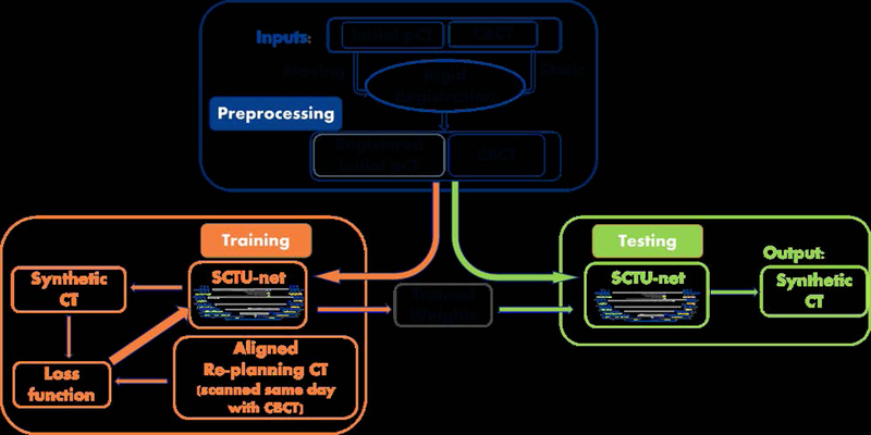
The pipeline of the proposed scheme for generating synthetic CT is illustrated in Figure 1. Even though exact deformable registration is not required between CBCT and the initial pCT in the proposed scheme, a rigid registration procedure was performed to speed up the convergence and obtain accurate synthesis. The 3D rigid registration between CBCT and the initial planning CT was performed by a commercial Velocity® software package (Varian Medical Systems, Palo Alto, CA). The initial pCT was aligned with CBCT, and the total time for both CBCT-pCT rigid registration and alignment matrix application on the previous pCT was around 2 minutes. CBCT and the registered pCT were then used as two inputs of the proposed sCTU-net. During the training stage, a deformable registration was performed between replanning CT and CBCT to generate a deformed replanning CT as a reference CT to form the loss function used during optimization. In the testing stage, CBCT and the registered initial pCT were directly fed into the well- trained sCTU-net to generate a synthetic CT, which has accurate CT numbers and the same anatomical structure as CBCT.
Figure 1:
Pipeline of the proposed scheme for generating synthetic CT.
2.3. Deep learning methods
The proposed sCTU-net is a U-net-based neural network that considers CBCT and registered previous pCT as inputs to generate synthetic CT images17. Building an effective neural network model dedicated to synthetic CT generation requires careful consideration of the network architecture and input format.
2.3.1. Image Normalization
To speed up the training convergence, we normalized the CBCT and registered pCT images to the range of [0, 1] according to the following formula:
| (1) |
where I indicates the original CBCT or registered pCT image whose range is [−1000, 3095]. This normalization operation preserves the original image contrast.
2.3.2. sCTU-net architecture
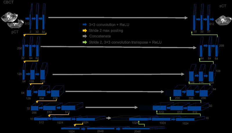
The architecture of the proposed sCTU-net is shown in Figure 2. CBCT and registered planning CT are two inputs of the proposed sCTU-net architecture. Information from both CBCT and pCT is integrated by the first convolutional layer with 32 different kernels. Another 13 convolutional layers and 6 max-pooling layers are alternatively arranged in the left part of sCTU-net to let convolutional kernels capture both local and global features in the image spatial domain. Then, another 13 convolutional layers and 6 up-sampling (convolution transpose) layers are designed in the right part of sCTU-net to preserve original image size and finally generate a synthetic CT image of the same size with the original CBCT image.
Figure 2:
Architecture of sCTU-net. The numbers below the blocks indicate the number of features for each map, and the numbers to the left of the blocks are the size of 2D feature outputs. The input data size is 512 × 512 × 2 and the output data size is 512 × 512 × 1.
The size of all the convolution kernels in the architecture is 3×3 and max-pooling layers are performed in 2-stride setting. Meanwhile, zero padding is also applied to any convolution, max-pooling, and up-sampling layer to maintain the output image size. As the slice dimension of the input image is 512×512 which can be exactly divisible by 2, the zero-padding size in the max-pooling layer is 0 in this study. Furthermore, the concatenating technique is applied for connecting the left and right part of the sCTU-net, which combines low-level features that contain detailed information with high-level features. To guarantee non-linearity, which indicates the complexity of the network, a rectified linear unit (ReLU) activation layer is equipped with each convolutional layer.
2.3.3. Loss function
The parameters embedded in the proposed sCTU-net are optimized by minimizing the loss error between the synthetic CT image and the aligned same-day-pCT image (reference CT image). We designed the loss error as a combination of mean-absolute-error (MAE) and structure dissimilarity (DSSIM) between the synthesized image and the reference image to enforce both pixel-wised and whole structure-wised similarity. Given a predicted synthetic CT (sCT) image and the corresponding reference CT (rCT) image, the loss function is designed as follows:
| (2) |
with
| (3) |
| (4) |
| (5) |
where α is a trade-off parameter between MAE and DSSIM, M is the total number of pixels in the sCT image, μ is the mean value of the image, σ is the standard variation of the image, and σx,y is the covariance of x and y two images. c1 and c2 are two variables that stabilize the division with a weak denominator. In our implementation, we set α = 0.75, c1 = (0.01L)2 and c2 = (0.03L)2 where L is the dynamic range of the pixel values in the rCT image.
2.3.4. Other sCTU-net settings
To investigate the influence of initial pCT on the final image quality of sCT, we used another setting of the sCTU-net in which only CBCT was used as the network input. Additionally, the influence of loss function was also investigated by setting the loss function as MAE alone, DSSIM alone, and a combination of MAE and DSSIM. We denoted the synthetic CT image obtained by using CBCT alone as input or combining CBCT with initial pCT as inputs like sCT-w/o-pCT-’loss’ or sCT-w-pCT-’loss’ where loss indicates the specific loss function such as mae, dssim and dssim&mae that was used for network training.
3. Experimental Results
3.1. Network training
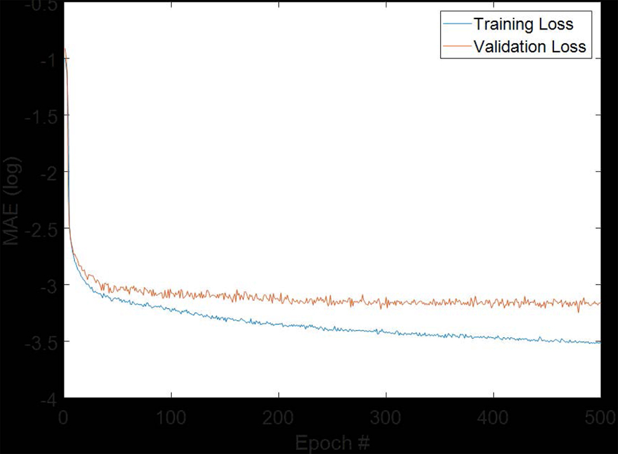
We used CBCT images and pCT images from 37 patients as a training dataset. Since 80 slices were available from each CBCT and pCT, 2960 slices of CBCT and reference CT images were present in the training dataset. We shuffled the 2960 slices into two parts with one including 2400 slices and the other including 560 slices. We used 2400 slices to train the proposed sCTU-net and the other 560 slices as validation dataset to tune the hypo-parameters of the proposed network, such as learning rate. For the final sCTU-net training, the Adam optimization algorithm was used with a learning rate of 1e-5 in Keras which was built on top of TensorFlow. We set the maximum training epoch number as 500 since the validation loss does not further decrease for more training steps. The training and validation loss are plotted in Figure 3. We selected the model with smallest validation loss as the optimal sCTU-net model. Then, we evaluated this optimal sCTU-net on the testing dataset that included 560 slices from 7 independent patients.
Figure 3:
Plot of training and validation loss with increasing epoch numbers.
3.2. Qualitative results
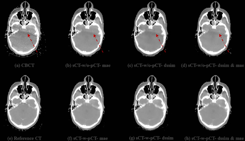
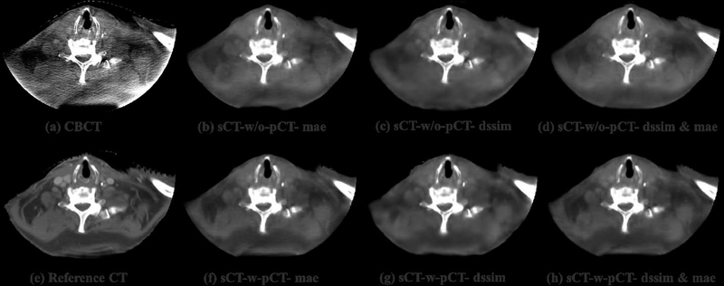
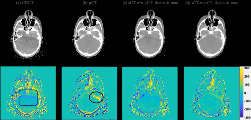
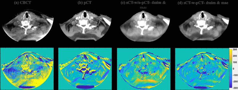
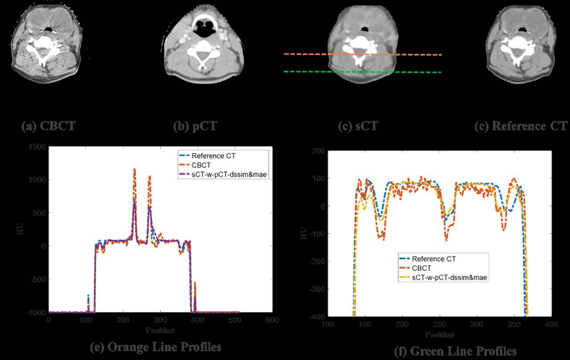
To visually evaluate the performance of the proposed synthetic CT generation network, we show the synthetic CT images obtained from the CBCT images (Figure 4 and Figure 6). The listed CBCT (Figure 4,6(a)) and reference CT images (Figure 4,6(e)) share the same structure, while the pCT images (Figure 5,7(b)) have much more different content structures than CBCT compared to the reference CT. Figure 4 and Figure 6 (b)–(d) list the synthetic CT images obtained by using CBCT alone as input, while (f)-(h) list the synthetic CT images obtained by using CBCT and previous pCT together as inputs. Less artifacts were found in all the generated sCT images than in the original CBCT. Compared with sCT-w/o-pCT images, sCT-w-pCT images can remove more artifacts, as indicated by the red arrow in Figure 4. Same conclusion can be drawn from the residual images between the sCT (w/o- or w-pCT) images and the reference CT image (Figure 5 and Figure 7). The bottom row images in Figure 5 also demonstrate that there is large difference between pCT and reference CT as compared to the corresponding difference between sCT-w-pCT-diss&mae and reference CT, as indicated by a circle. The line profiles of CT numbers of CBCT, sCT-w-pCT-dssim&mae, and reference CT were also plotted in Figure 8. For the same soft tissue region, the CT number of CBCT has stronger volatility than that of reference CT. The CT numbers of sCT image are much closer to those of reference CT than those of CBCT.
Figure 4:
Testing sample one of sCTU-net. (a) CBCT image; (e) reference CT image obtained by deformable registration; (b-(d) synthetic CT images obtained by sCTU-net with CBCT alone as input; (f)-(h) synthetic CT images obtained by sCTU-net with initial pCT and CBCT both as inputs.
Figure 6:
Testing sample two of sCTU-net. (a) CBCT image; (e) reference CT image obtained by deformable registration; (b-(d) synthetic CT images obtained by sCTU-net with CBCT alone as input; (f)-(h) synthetic CT images obtained by sCTU-net with initial pCT and CBCT both as inputs.
Figure 5:
CBCT, initial pCT, sCT-w/o-pCT-dssim&mae and sCT-w-pCT-dssim&mae images and the corresponding residual images between these images and the reference CT image for testing sample one.
Figure 7:
CBCT, initial pCT, sCT-w/o-pCT-dssim&mae and sCT-w-pCT-dssim&mae images and the corresponding residual images between these images and the reference CT image for testing sample two.
Figure 8:
Example showing HU line profiles of CBCT, sCT, and reference CT.
3.3. Quantitative analysis
Four evaluation criteria including MAE, root-mean-square-error (RMSE), peak-signal-noise-ratio (PSNR), and SSIM were used to evaluate the performance of different synthetic image generation models from pixel-wise HU accuracy, noise level, and structure similarity. Given two images I1 and I2 with the total number of pixels in each image as M, we provide the following definition and detailed formulas for these criteria:
MAE: MAE is used to calculate the mean absolute error of all the pixel values in two images. The MAE formula is shown in Eq. (3). Lowering MAE improves image quality.
- RMSE: RMSE is a frequently used measure of the differences between values predicted by a model or an estimator and the values observed. Lowering RMSE improves image quality.
(6) - PSNR: PSNR is a metric commonly used to evaluate image quality, especially for noise reduction, which is a combination of the mean squared error and maximum intensity value of the reference image. Increasing PSNR improves image quality.
where If is the reference image of I1 and I2.(7) SSIM: Structural information is essentially considered in SSIM to compare the quality of the predicted image with that of the reference image. The formula of SSIM is shown in Eq. (5). Increasing SSIM improves image quality. In this study, SSIM values were calculated over the patient anatomical regions by excluding background for evaluating anatomy structure similarity.
Note that we converted the normalized synthetic CT intensity value back to HU range of [−1000, 3095] by multiplying 4095 and then subtracting 1000 for the following quantitative comparisons. The values of the four evaluation criteria obtained by different sCTU-net settings are listed in Table 1. Using initial pCT as the input can generate sCT of higher image quality than the network using CBCT as the input alone. Additionally, although MAE used alone as loss function can improve HU accuracy to some extent, a combination of MAE and DSSIM can generate better CT-like images.
Table 1:
Evaluation criteria values obtained by different settings of sCTU-net
| SSIM | PSNR | MAE | RMSE | |
|---|---|---|---|---|
| CBCT | 0.7109 | 27.35 | 44.38 | 126.43 |
| pCT | 0.8134 | 27.82 | 32.47 | 105.85 |
| sCT-w/o-pCT-mae | 0.8852 | 32.72 | 21.89 | 64.87 |
| Relative improvement (%) | 24.52% | 19.63% | 50.68% | 48.69% |
| sCT-w/o-pCT-dssim | 0.8850 | 32.38 | 23.50 | 68.11 |
| Relative improvement (%) | 24.49% | 18.39% | 47.05% | 46.13% |
| sCT-w/o-pCT-dssim&mae | 0.8880 | 32.69 | 21.68 | 65.05 |
| Relative improvement (%) | 24.91% | 19.52% | 51.15% | 48.55% |
| sCT-w-pCT-mae | 0.8875 | 33.19 | 19.17 | 64.08 |
| Relative improvement (%) | 24.84% | 21.35% | 56.80% | 49.32% |
| sCT-w-pCT-dssim | 0.8874 | 32.61 | 20.37 | 62.28 |
| Relative improvement (%) | 24.83% | 19.23% | 54.10% | 50.74% |
| sCT-w-pCT-dssim&mae | 0.8911 | 33.26 | 18.98 | 60.16 |
| Relative improvement (%) | 25.35% | 21.61% | 57.23% | 52.42% |
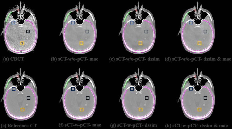
As the CT number accuracy of the soft-tissue region is relevant for patient set-up and dose calculation, we also calculated the mean CT numbers and standard deviations (std) for some soft tissue regions of interest (ROI) in CBCT and synthetic CT images to demonstrate the efficacy of the proposed sCTU-net. The three ROIs (ROI 1, 2 and 3) selected to evaluate the uniformity of the soft tissue HU values are shown in Figure 9. Additionally, another three ROIs (ROI 4, 5 and 6) for bone regions are also shown in Figure 9 to demonstrate the agreement of CT numbers between synthetic CT and reference CT. We list the mean ± std CT numbers of the selected ROIs in CBCT, synthetic CT, and reference CT for soft tissue and bone regions in Table 2. The mean CT numbers of the sCT images are much closer to those of the reference CT image than those of the original CBCT image. Moreover, the standard variations of the soft tissue CT numbers in the sCT images are closer to that of the reference CT image than that of CBCT. Overall, the mean and standard deviation of CT numbers in the sCT-w-pCT-dssim&mae are closest to the reference image.
Figure 9:
Example showing the three selected 11 by 11 ROIs (ROI 1, 2 and 3) for soft tissues and three selected ROIs (ROI 4, 5 and 6) for bone in CBCT, synthetic CT, and reference CT.
Table 2:
Comparison of CT number accuracy of soft tissue and bone regions in CBCT, synthetic CT, and reference CT.
| ROI No. | 1 | 2 | 3 | 4 | 5 | 6 |
|---|---|---|---|---|---|---|
| Reference CT | 53±4 | 52±5 | 54±3 | 995±260 | 819±178 | 1023±245 |
| CBCT | 132±36 | 100±40 | 104±34 | 1422±405 | 1316±369 | 1332±410 |
| sCT-w/o-pCT-mae | 103±4 | 80±2 | 74±6 | 954±239 | 809±201 | 1009±236 |
| sCT-w/o-pCT-dssim | 62±8 | 39±5 | 25±7 | 944±246 | 769±184 | 998±259 |
| sCT-w/o-pCT-dssim&mae | 85±5 | 65±3 | 64±7 | 980±243 | 821±193 | 1054±268 |
| sCT-w-pCT-mae | 58±3 | 51±4 | 56±4 | 987±272 | 833±197 | 1045±246 |
| sCT-w-pCT-dssim | 54±5 | 53±4 | 56±3 | 1224±196 | 821±193 | 1027±258 |
| sCT-w-pCT-dssim&mae | 53±4 | 51±3 | 55±3 | 997±258 | 818±176 | 1026±246 |
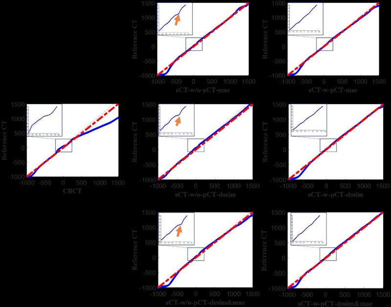
We also displayed the quantile-quantile (Q-Q) plot between CBCT (synthetic CT) and reference CT to compare the CT number distributions in these images (Figure 10). The closer the blue curve is to the red line y=x, the better agreement between the distributions is expected. The points in the Q-Q plot for comparing synthetic CT with reference CT almost lie around the straight line y=x, while large shift is observed between points in the Q-Q plot for comparing CBCT with reference CT and y=x. The CT number distribution of the synthetic CT is more similar to that of reference CT than CBCT. The left-upper blue box in each subplot of Figure 10 contains the zoomed Q-Q plot in region of [−300, 300]. The Q-Q plots of sCT-w-pCT images don’t have the concavities as indicated by the orange arrows shown in the plots of sCT-w/o-pCT images. These results demonstrate that the model with initial pCT as the prior image achieves better results than using CBCT alone as input, especially in the soft-tissue region.
Figure 10:
Quantile-quantile plots of CBCT (1st column), sCT-w/o-pCT (2nd column) and sCT-w-pCT (3rd column) with reference CT.
3.3. Generalizability of H&N model (sCT-w/o-pCT) on pelvic region
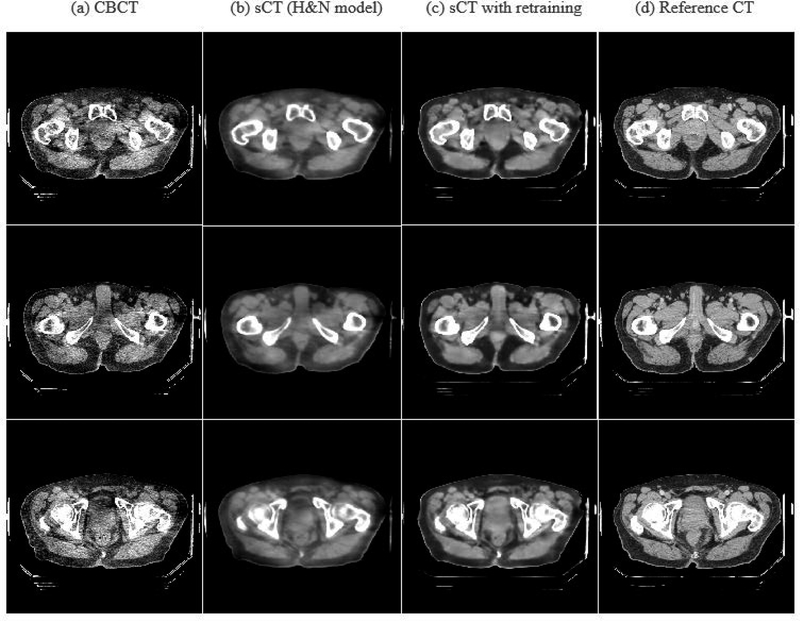
Correcting HU value for CBCT of pelvic region is more challenging since larger fraction of scatter signal presents in pelvic CBCT than H&N CBCT. We performed two experiments to test the model generalizability of the H&N model for the pelvic region. Note that replanning for prostate radiation therapy is very rare; thus the same day replanning CTs are not available for model training and evaluation in the prostate case. Hence, in this study, we can only evaluate the generalizability of the H&N sCT-w/o-pCT model for the prostate site with using the deformed initial pCT as the reference CT for model training. We first applied the model (sCT-w/o-pCT) trained on the H&N dataset to the pelvic CBCT directly. The results of direct H&N model are shown in Figure 11 (column 2) and Table 3 (row 3). These results showed that the proposed model trained for H&N site can produce reasonable sCT with much higher quality than CBCT. We then further fine-tuned18,19 the model (sCT-w/o-pCT) by retraining the model using a limited number of pelvic images from six patients. We set the maximum epoch for fine-tuning as 200 and selected the model with the smallest validation loss as the optimal sCTU-net model for the pelvic CBCT. The results of this transfer learning strategy can also be found in Figure 11 and Table 3. While the original H&N model (without retraining) obtains reasonable results, fine-tuning of the original model is preferred to achieve improved results for other anatomical sites.
Figure 11:
CBCT, sCTs, and reference CT images around pelvic region.
Table 3:
Evaluation criteria values obtained by sCTU-net for pelvic data
| SSIM | PSNR | MAE | RMSE | |
|---|---|---|---|---|
| CBCT | 0.8897 | 27.59 | 104.21 | 163.71 |
| sCT (H&N model) | 0.9373 | 32.08 | 46.78 | 99.31 |
| sCT with retraining | 0.9405 | 32.83 | 42.40 | 94.06 |
4. Discussions and Conclusion
We formulated the CT synthesis problem under a deep learning framework, where a deep U-net architecture was employed to take advantage of the anatomical structure of on-treatment CBCT and image intensity information of initial pCT. Original CBCT and initial pCT are two inputs of the network. U-net was chosen because of its ability of using both global and local features in the image spatial domain, suppressing global scattering and local artifacts (e.g., CBCT noise). A combination of DSSIM and MAE was selected as loss function for network training because it considers both pixel-wise whole image HU accuracy and structural information.
In the supervised learning models developed in this work, ideally, we would employ a replanning CT with identical anatomical structure with CBCT as reference to train the proposed model. However, such an ideal CBCT-CT pair is not readily available as they are not acquired simultaneously. In this study, we identified H&N patients having replanning CT taken on the same day (same-day pCT) as the CBCT. Thus the anatomical structure is almost identical between the same-day pCT and CBCT. However, as CBCT and same-day pCT were not scanned simultaneously, small amount of deformation were observed. A 3D deformable multi-pass registration between CBCT and this same-day pCT was then performed for optimal performance. H&N cancer site has a bigger chance requiring replanning as the change of tumor (i.e., tumor shrinking) could be observed during a treatment course20. Therefore, in this work, we mainly focused on the H&N cancer. For other disease sites, such as prostate cancer, replanning is rare. As such, replanning CT acquired on the same day as CBCT is not available for model training. In the experiment to test model generalizability of H&N sCT-w/o-pCT for the prostate, we used deformed initial pCT as the reference CT for model training and evaluation for the pelvic region. Unsupervised learning strategy would be preferred for these cases in a future study.
Our results show that the synthetic CT images have good image quality, as indicated by lower noise and artifacts. The CT number in CBCT was successfully corrected by the proposed scheme. Moreover, the synthetic CT images have greater geometry-match than deformed CT with original CT, indicating that generating a straightforward synthetic CT image may be better than deforming CT images through DIR, especially when the patient’s imaging content changes during the whole treatment course.
The goal of this work is to synthesize CT for replanning purpose from on-treatment CBCT. In our implementation, we firstly upsampled pCT to CBCT resolution mainly because CBCT has higher resolution (0.5112 mm×0.5112 mm×1.9897mm vs 1.1719mm×1.1719 mm×3mm in pCT). This way, patients’ updated geometrical information from CBCT can be maintained with high fidelity (by avoiding downsampling) while the CT number information from pCT is not affected much by upsampling. After sCT is generated using the proposed sCTU-net, we are able to simply downsample the sCT back to the same resolution of pCT. Thus the purpose of replanning using sCT can be fully realized using the proposed workflow.
The model developed in this work is 2D, which generates sCT in a slice-by-slice fashion. Volumetric neural network21–24 could help to enhance the performance of the 2D model. However, the required model size is significantly larger than the current 2D model, which is beyond our hardware capability and requires more training samples. A further study is warranted to evaluate the gain using a volumetric neural network.
In summary, we proposed a scheme that generates a synthetic CT image from CBCT, preserving geometry information of the original CBCT with accurate CT numbers. Our system can increase the accuracy of CT number of CBCT, which allows further quantitative applications of CBCT, such as dose calculation and adaptive treatment planning.
5. Acknowledgement
This work was supported in part by the Cancer Prevention and Research Institute of Texas (RP160661) and US National Institutes of Health (R01 EB020366).
6. Reference
- 1.Sorcini B, Tilikidis A. Clinical application of image-guided radiotherapy, IGRT (on the Varian OBI platform). Cancer/Radiothérapie. 2006;10(5):252–257. [DOI] [PubMed] [Google Scholar]
- 2.Boda-Heggemann J, Lohr F, Wenz F, Flentje M, Guckenberger M. kV cone-beam CT-based IGRT. Strahlentherapie und Onkologie 2011;187(5):284–291. [DOI] [PubMed] [Google Scholar]
- 3.Jaju PP, Jain M, Singh A, Gupta A. Artefacts in cone beam CT. Open Journal of Stomatology 2013;3(05):292. [Google Scholar]
- 4.Schulze R, Heil U, Groβ D, et al. Artefacts in CBCT: a review. Dentomaxillofacial Radiology 2011;40(5):265–273. [DOI] [PMC free article] [PubMed] [Google Scholar]
- 5.Wang H, Dong L, Lii MF, et al. Implementation and validation of a three-dimensional deformable registration algorithm for targeted prostate cancer radiotherapy. International Journal of Radiation Oncology* Biology* Physics 2005;61(3):725–735. [DOI] [PubMed] [Google Scholar]
- 6.Zhu L, Xie Y, Wang J, Xing L. Scatter correction for cone‐beam CT in radiation therapy. Medical physics 2009;36(6Part1):2258–2268. [DOI] [PMC free article] [PubMed] [Google Scholar]
- 7.Xu Y, Bai T, Yan H, et al. A practical cone-beam CT scatter correction method with optimized Monte Carlo simulations for image-guided radiation therapy. Physics in Medicine & Biology 2015;60(9):3567. [DOI] [PMC free article] [PubMed] [Google Scholar]
- 8.Wu M, Keil A, Constantin D, Star‐Lack J, Zhu L, Fahrig R. Metal artifact correction for x‐ray computed tomography using kV and selective MV imaging. Medical physics 2014;41(12). [DOI] [PMC free article] [PubMed] [Google Scholar]
- 9.Bechara B, Moore W, McMahan C, Noujeim M. Metal artefact reduction with cone beam CT: an in vitro study. Dentomaxillofacial Radiology 2012;41(3):248–253. [DOI] [PMC free article] [PubMed] [Google Scholar]
- 10.Li Y, Garrett J, Chen G-H. Reduction of beam hardening artifacts in cone-beam CT imaging via SMART-RECON algorithm. Paper presented at: Medical Imaging 2016: Physics of Medical Imaging2016. [DOI] [PMC free article] [PubMed] [Google Scholar]
- 11.Xie S, Zhuang W, Li H. An energy minimization method for the correction of cupping artifacts in cone‐beam CT. Journal of applied clinical medical physics 2016;17(4):307–319. [DOI] [PMC free article] [PubMed] [Google Scholar]
- 12.Wei Z, Guo-Tao F, Cui-Li S, et al. Beam hardening correction for a cone-beam CT system and its effect on spatial resolution. Chinese Physics C 2011;35(10):978. [Google Scholar]
- 13.Zhang Y, Yu H. Convolutional Neural Network based Metal Artifact Reduction in X-ray Computed Tomography. IEEE transactions on medical imaging 2018;37(6):1370–1381. [DOI] [PMC free article] [PubMed] [Google Scholar]
- 14.Xu S, Prinsen P, Wiegert J, Manjeshwar R. Deep residual learning in CT physics: scatter correction for spectral CT. arXiv preprint arXiv:170804151 2017. [Google Scholar]
- 15.Yan H, Zhen X, Cerviño L, Jiang SB, Jia X. Progressive cone beam CT dose control in image‐guided radiation therapy. Medical physics 2013;40(6Part1). [DOI] [PMC free article] [PubMed] [Google Scholar]
- 16.Ronneberger O, Fischer P, Brox T. U-net: Convolutional networks for biomedical image segmentation. Paper presented at: International Conference on Medical image computing and computer-assisted intervention2015. [Google Scholar]
- 17.Çiçek Ö, Abdulkadir A, Lienkamp SS, Brox T, Ronneberger O. 3D U-Net: learning dense volumetric segmentation from sparse annotation. Paper presented at: International Conference on Medical Image Computing and Computer-Assisted Intervention2016. [Google Scholar]
- 18.Shie C-K, Chuang C-H, Chou C-N, Wu M-H, Chang EY. Transfer representation learning for medical image analysis. Paper presented at: 2015 37th annual international conference of the IEEE Engineering in Medicine and Biology Society (EMBC)2015. [DOI] [PubMed] [Google Scholar]
- 19.Chang J, Yu J, Han T, Chang H-j, Park E A method for classifying medical images using transfer learning: a pilot study on histopathology of breast cancer. Paper presented at: 2017 IEEE 19th International Conference on e-Health Networking, Applications and Services (Healthcom) 2017.
- 20.Hansen EK, Bucci MK, Quivey JM, Weinberg V, Xia P. Repeat CT imaging and replanning during the course of IMRT for head-and-neck cancer. International Journal of Radiation Oncology* Biology* Physics. 2006;64(2):355–362. [DOI] [PubMed] [Google Scholar]
- 21.Roth HR, Lu L, Lay N, et al. Spatial aggregation of holistically-nested convolutional neural networks for automated pancreas localization and segmentation. Medical image analysis 2018;45:94–107. [DOI] [PubMed] [Google Scholar]
- 22.Casamitjana A, Puch S, Aduriz A, Sayrol E, Vilaplana V. 3d convolutional networks for brain tumor segmentation. Proceedings of the MICCAI Challenge on Multimodal Brain Tumor Image Segmentation (BRATS) 201665–68. [Google Scholar]
- 23.Kearney VP, Chan JW, Wang T, Perry A, Yom SS, Solberg TD. Attention-enabled 3D boosted convolutional neural networks for semantic CT segmentation using deep supervision. Physics in Medicine & Biology 2019. [DOI] [PubMed] [Google Scholar]
- 24.Wang Y, Teng Q, He X, Feng J, Zhang T. CT-image Super Resolution Using 3D Convolutional Neural Network. arXiv preprint arXiv:180609074 2018. [Google Scholar]


