Registration Uncertainty Quantification Via Low-dimensional Characterization of Geometric Deformations

Abstract

This paper presents an efficient approach to quantifying image registration uncertainty based on a low-dimensional representation of geometric deformations. In contrast to previous methods, we develop a Bayesian diffeomorphic registration framework in a bandlimited space, rather than a high-dimensional image space. We show that a dense posterior distribution on deformation fields can be fully characterized by much fewer parameters, which dramatically reduces the computational complexity of model inferences. To further avoid heavy computation loads introduced by random sampling algorithms, we approximate a marginal posterior by using Laplace’s method at the optimal solution of log-posterior distribution. Experimental results on both 2D synthetic data and real 3D brain magnetic resonance imaging (MRI) scans demonstrate that our method is significantly faster than the state-of-the-art diffeomorphic registration uncertainty quantification algorithms, while producing comparable results.

1. Introduction

Diffeomorphic Image registration is a fundamental tool in image analysis as it provides one-to-one smooth and invertible smooth spatial correspondences (also known as diffeomorphisms) between pairwise images. Examples of applications include alignment of functional data to a reference coordinate system [1, 2], anatomical comparisons across individuals [3, 4], and atlas-based image segmentation [5, 6]. In general, image registration is an ill-posed problem since the image data are usually contaminated by unknown noise. Therefore, developing efficient measures to quantify the registration uncertainty or error is critical to fair assessments on estimated transformations, as well as subsequent improvement on the accuracy of predictive models. This also forms the basis for model-assisted decision making, for example, image-guided navigation system for neurosurgery [7, 8]. An efficient uncertainty quantification can provide important information on brain shifts (deformations) for neurosurgeons to identify residual tumor tissues during surgery; hence leading to a significant increase in the extent of tumor removal while lowering the risk of collateral tissue damage.

Existing methods have been investigated to estimate the uncertainty by having a probability distribution over the latent space of transformation parameters either in a small or large deformation setting [9, 10]. These approaches formulate Bayesian image registration as an image matching likelihood term regularized by a prior that guarantees the smoothness of deformation fields. A posterior distribution is then generated as a measure of the registration uncertainty estimation. Due to the fact that such posterior distributions do not have closed-form formulations, stochastic and sampling methods typically have been employed [11, 12, 7]. This makes the entire inference extremely challenging on a dense image grid (e.g., a 3D brain MRI with the size of 128³). Large computational resources and efforts are required to sample over a high-dimensional space with extremely slow convergence. Also, none of the aforementioned algorithms is able to compute a full posterior covariance. These disadvantages dramatically decrease the model usability in important applications that require computational efficiency.

In this paper, we propose an efficient registration uncertainty quantification model that employs a low-dimensional representation of diffeomorphic transformations [13, 14]. Based on the key fact that the tangent space of diffeomorphisms do not develop high frequencies, we develop a Bayesian registration framework entirely in a bandlimited space with low frequencies well preserved. A posterior distribution of transformation fields is carefully designed in a truncated frequency domain, where all diffeomorphic properties remain valid. Similar to [15], we derive a Laplace approximation of the log-posterior distribution at an optimal solution to further avoid intensive computation cost of sampling methods. More specifically, we assume a complex Gaussian distribution at the mode of the posterior, with its covariance estimated by second-order information to describe uncertainties in the registration model. This is effectively done by computing an inverse Hessian of the log-posterior specifically defined in a low-dimensional bandlimited space. Our model dramatically reduces the computational complexity of approximating posterior marginals in the space of diffeomorphisms, which makes registration uncertainty analysis tractable in time. In practical, the efficiency of our method strengthens its feasibility in prospective clinical applications under a tight time constraint. This paper is an extension of a recently published conference paper [16] with (i) in-depth derivations of the Hessian computation and inference procedure provided; and (ii) comprehensive experiments to thoroughly validate the method included. We run tests on both 2D synthetic data and real 3D brain MRI scans from OASIS dataset [17]. We then compare estimated results with the state-of-the-art registration uncertainty quantification method in the full image space [15]. Experimental results show that our method is significantly faster than the baseline algorithm, while producing comparable results.

The rest of this paper is structured as follows. Sec. 2 briefly introduces the background of diffeomorphic image registration in the context of large deformation diffeomorphic metric mapping (LDDMM) framework [18] followed by a Fourier representation of diffeomorphisms [13, 19]. Sec. 3 introduces our developed Bayesian model with Sec. 4 presenting the inference. Sec. 5 demonstrates our experiments with detailed discussions.

2. Background

In this section, we first briefly review the background of diffeomorphic image registration in the context of LDDMM with geodesic shooting algorithm [18, 20]. We then introduce a recently developed Fourier representation of velocity fields in the tangent space of diffeomorphisms that dramatically speeds up the registration optimization [13, 19].

2.1. LDDMM With Geodesic Shooting

Let S be a source image and T be a target image defined on a torus domain $\mathrm{\Gamma }={ℝ}^d/{\mathbb{Z}}^d(S(x),T(x):\mathrm{\Gamma }\to ℝ)$. The problem of diffeomorphic image registration is to find the shortest path to generate time-varying diffeomorphisms {ψ_t} : t ∈ [0, 1] such that S ∘ ψ₁ is similar to T, where ∘ is a composition operator that resamples S by the smooth mapping ψ₁. This is typically solved by minimizing an explicit energy function of LDDMM [18] as

$$E\left(v_t\right)=\mathrm{dist}\left(S\circ {\psi }_1,T\right)+\left(\mathcal{L}{v}_t,v_t\right),s.t.\frac{d{\psi }_t}{dt}=-\mathcal{D}{\psi }_t\cdot v_t,$$ (1)

where the distance function dist(·, ·) measures the dissimilarity between images. Commonly used distance functions include sum-of-squared difference of image intensities [18], normalized cross correlation [21], and mutual information [22].The regularization term $\left(\mathcal{L}{v}_t,v_t\right)$ is a constraint that enforces spatial smoothness of transformations with $\mathcal{L}$ being a symmetric and positive-definite differential operator. Here, (·,·) denotes a pair between a tangent vector v_t and a momentum vector $m_t=\mathcal{L}{v}_t$ that is similar to an inner product, $\mathcal{D}$ is a Jacobian matrix, and · is an element-wise multiplication.

The geodesic shooting algorithm states that, given an initial velocity v₀, a shortest path of diffeomorphisms {ψ_t} can be uniquely determined by integrating the geodesic evolution equation (also known as Euler-PoincarÃl’ differential equation (EPDiff) [23, 24]) as

$$\frac{d{v}_t}{dt}={\text{ad}}_{v_t}^{†}{v}_t=-\mathcal{K}\left[{\left(\mathcal{D}{v}_t\right)}^T\cdot m_t+\mathcal{D}{m}_t\cdot v_t+m_t\cdot \mathrm{div}{v}_t\right],$$ (2)

where ad^† is an adjoint operator, $\mathcal{K}$ is an inverse operator of $\mathcal{L}$, and div denotes the divergence.

As a consequence, the optimization of LDDMM with geodesic shooting can be equivalently written as

$$E\left(v_0\right)=\mathrm{dist}\left(S\circ {\psi }_1,T\right)+\left(\mathcal{L}{v}_0,v_0\right),s.t.\frac{d{\psi }_t}{dt}=-D{\psi }_t\cdot v_t\&\text{Eq.}(2).$$ (3)

This substantially reduces the computational complexity and improves the optimization landscape by only manipulating the initial velocity v₀ with EPDiff in Eq. 2, rather than the entire time-dependent velocity fields v_t.

2.2. Fourier Representation of Velocity Fields

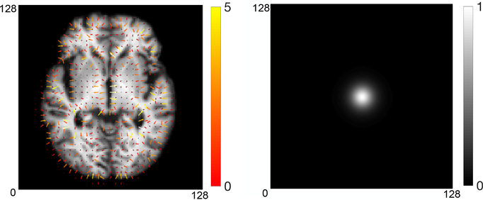
A recent work has shown that the velocity fields generated by EPDiff (2) can be efficiently captured via a low-dimensional representation in Fourier space with bandlimited signals [13, 19]. The key idea behind is that the velocity fields do not develop high frequencies and only a small amount of low frequencies contributes to the computation of generating deformation fields (as shown in Fig. 1). Therefore, we are able to capture the deformations in a bandlimited space as accurately as the original space. We next briefly review the relevant details of the method.

Figure 1:

Left to right: an example of 2D velocity field visualized in image space vs. Fourier space. The white dot centered in middle displays centered low frequencies.

Let $f:{ℝ}^d\to ℝ$ be a real-valued function. The Fourier transform $\mathcal{F}$ of f is given by

$$\mathcal{F}[f](\xi )={\int }_{{ℝ}^d}f(x)e^{-2\pi i\langle \xi ,x\rangle }dx,$$ (4)

where x = (x₁, …, x_d) is a d-dimensional vector of image coordinates, ξ = (ξ₁, …,ξ_d) is a d-dimensional vector of frequencies, and 〈·, ·〉 denotes an inner product operator. The inverse Fourier transform ${\mathcal{F}}^{-1}$ of a discretized Fourier signal $\tilde{f}$

$${\mathcal{F}}^{-1}[\tilde{f}](x)=\sum _{\xi }\tilde{f}(\xi )e^{2\pi i\langle \xi ,x\rangle }$$ (5)

is an approximation of the original signal f. For vector-valued functions, such as diffeomorphisms ψ and velocity fields v, we apply (inverse) Fourier transform to each vector component separately.

Analogous to the EPDiff defined on the spatial domain of image space, we rewrite Eq. (2) in frequency domain as

$$\frac{\partial {\tilde{v}}_t}{\partial t}={\mathrm{ad}}_{{\tilde{v}}_t}^{†}{\tilde{v}}_t=-\tilde{\mathcal{K}}\left[{\left(\tilde{\mathcal{D}}{\tilde{v}}_t\right)}^T\star {\tilde{m}}_t+\tilde{\mathcal{D}}{\tilde{m}}_t\ast {\tilde{v}}_t+{\tilde{m}}_t\ast \left(\tilde{\nabla }\cdot {\tilde{v}}_t\right)\right],$$ (6)

where $\tilde{\mathcal{K}}$ is a smoothing operator. Here $\tilde{\mathcal{L}}$ is the Fourier coefficients of a differential operator $\mathcal{L}$, which converts a vector field $\tilde{v}$ to a momentum vector by $\tilde{m}=\tilde{\mathcal{L}}\tilde{v}$, ⋆ is a circular matrix-vector field auto-correlation ¹, ∗ is a circular convolution, and $\tilde{\mathcal{D}}\tilde{v}$ is a tensor product $\tilde{D}\otimes \tilde{v}$ with $\tilde{D}(\xi )=i\sin (2\pi \xi )$ representing the Fourier frequencies of a central difference Jacobian matrix D. The operator $\tilde{\nabla }$ is the discrete divergence operator that is computed as the sum of the Fourier coefficients of the central difference operator $\tilde{D}$ along each dimension, i.e., $\tilde{\nabla }\cdot \xi =\sum _{j=1}^{d}i\sin \left(2\pi {\xi }_j\right)$.

Since $\mathcal{K}$ on the left side of Eq. (6) is a smoothing operator (low-pass filter) that suppresses high frequencies in the Fourier domain, all computational operations in (6) are easy to implement in a truncated low-dimensional space by eliminating high frequencies. To ensure that $\tilde{f}$ represents a real-valued vector field in the spatial domain, we require $\tilde{f}\left({\xi }_1,\dots ,{\xi }_d\right)={\tilde{f}}^{*}\left(-{\xi }_1,\dots ,-{\xi }_d\right)$, where ^∗ denotes the complex conjugate.

Similarly, the diffeomorphic transformations in the frequency domain can be computed by

$$\begin{gathered} \frac{d{\tilde{\psi }}_t}{dt}=-\tilde{\mathcal{D}}{\tilde{\psi }}_t\ast {\tilde{v}}_t,\text{or} \\ \frac{d{\tilde{u}}_t}{dt}=-{\tilde{v}}_t-\tilde{\mathcal{D}}{\tilde{u}}_t\ast {\tilde{v}}_t\text{with}{\tilde{\psi }}_t=\tilde{e}+{\tilde{u}}_t, \end{gathered}$$ (7)

where $\tilde{e}$ is the fourier coefficients of an identity element of image coordinates.

3. Our Model: Low-dimensional Bayesian Registration Uncertainty Quantification

We introduce a low-dimensional Bayesian model of diffeomorphic image registration represented in the bandlimited velocity space $\tilde{V}$, with registration uncertainty explicitly encoded as latent variables of the model.

Assuming independent and identically distributed (i.i.d.) Gaussian noise on image intensities, we obtain the likelihood

$$p\left(T|S,{\sigma }^2\right)=\frac{1}{{\left(\sqrt{2\pi }{\sigma }^2\right)}^M}\exp \left(-\frac{1}{2{\sigma }^2}{\Vert S\circ {\psi }_1-T\Vert }_2^2\right),$$ (8)

where σ² is the noise variance and M is the number of image voxels. The deformation ψ₁ corresponds to ${\tilde{\psi }}_1$ in Fourier space via the Fourier transform $\mathcal{F}\left({\psi }_1\right)={\tilde{\psi }}_1$, or its inverse ${\psi }_1=\mathcal{F}\left({\tilde{\psi }}_1\right)$.

We define a prior on the initial velocity field ${\tilde{v}}_0$ to be a complex multivariate Gaussian distribution that ensures the smoothness of the geodesic path, i.e.,

$$p\left({\tilde{v}}_0\right)=\frac{1}{{(2\pi )}^{\frac{Md}{2}}{\left|{\tilde{\mathcal{L}}}^{-1}\right|}^{\frac{1}{2}}}\exp \left(-\frac{1}{2}(\tilde{\mathcal{L}}{\tilde{v}}_0,{\tilde{v}}_0)\right),$$ (9)

where |·| is matrix determinant. In this paper, we define $\tilde{\mathcal{L}}$ as the Fourier coefficients of a commonly used Laplacian operator $\mathcal{L}={(-\alpha \mathrm{\Delta }+I)}^c$ with a positive weight parameter α and a smoothness parameter c. The Fourier transform of the Laplacian operator is given by

$$\tilde{\mathcal{L}}(\xi )={\left(-2\alpha \sum _{j=1}^d\left(\cos \left(2\pi {\xi }_j\right)-1\right)+1\right)}^c,$$

with $\tilde{\mathcal{K}}=1/\tilde{\mathcal{L}}$ being an inverse operator of $\tilde{\mathcal{L}}$.

Combining the likelihood (8) and prior (9) together, we obtain the negative log posterior distribution on the deformation parameter parameterized by ${\tilde{v}}_0$ as

$$-\ln p\left({\tilde{v}}_0|S,T,{\sigma }^2\right)=\frac{1}{2}\left(\tilde{\mathcal{L}}{\tilde{v}}_0,{\tilde{v}}_0\right)+\frac{{\Vert S\circ {\psi }_1-T\Vert }_2^2}{2{\sigma }^2}+M\ln \sigma +\text{const}.$$ (10)

In most probabilistic formulations of image-based registration, the likelihood function (8), as a function of the transformation parameters, is highly non-Gaussian because of the complex spatial structure of the images. This brings difficulties in the inference of such a non-Gaussian posterior. While sampling methods have been investigated to empirically approximate the distribution [25, 26], the computation tends to be extremely time-consuming and expensive. To address this issue, we next introduce Laplace’s method [27] to approximate the posterior distribution in a much more efficient manner.

3.1. Laplace approximation

The basic idea is to find the mode of the posterior as a MAP solution, and then apply a second-order Taylor series approximation for the log-posterior function that corresponds to a complex Gaussian distribution. We first minimize the negative log posterior in (10) to the optimum ${\tilde{v}}_0^{opt}$, which is considered to be the mean of the Gaussian distribution (details of inference will be introduced in Sec. 4). Estimation of covariance is not straightforward, as we will need to derive a quadratic function of log-posterior by second-order approximation.

To simplify the notation, we use $f\left({\tilde{v}}_0\right)\triangleq -\ln p\left({\tilde{v}}_0|S,T,{\sigma }^2\right)$ to represent the log-posterior. The function $f\left({\tilde{v}}_0\right)$ is approximated to quadratic order by using second order Taylor series expansion at the optimal solution ${\tilde{v}}_0$ as

$$\begin{gathered} f\left({\tilde{v}}_0\right)=f\left({\tilde{v}}_0^{opt}+\left({\tilde{v}}_0-{\tilde{v}}_0^{opt}\right)\right) \\ \approx f\left({\tilde{v}}_0^{opt}\right)+\nabla f^T\left({\tilde{v}}_0^{opt}\right)\left({\tilde{v}}_0-{\tilde{v}}_0^{opt}\right)+\frac{1}{2}{\left({\tilde{v}}_0-{\tilde{v}}_0^{opt}\right)}^T\mathcal{H}f\left({\tilde{v}}_0^{opt}\right)\left({\tilde{v}}_0-{\tilde{v}}_0^{opt}\right), \end{gathered}$$

where ∇ denotes the first derivative and $\mathcal{H}$ is a second-order Hessian. Since the first derivative of f vanishes at the optimal solution ${\tilde{v}}_0^{opt}$, we have

$$f\left({\tilde{v}}_0\right)\approx f\left({\tilde{v}}_0^{opt}\right)+\frac{1}{2}{\left({\tilde{v}}_0-{\tilde{v}}_0^{opt}\right)}^T\mathcal{H}f\left({\tilde{v}}_0^{opt}\right)\left({\tilde{v}}_0-{\tilde{v}}_0^{opt}\right).$$ (11)

This indicates that the posterior is approximately a multivariate Gaussian distribution $\mathcal{N}\left({\tilde{v}}_0^{opt},{\mathcal{H}}^{-1}f\left({\tilde{v}}_0^{opt}\right)\right)$. The optimal solution ${\tilde{v}}^{opt}$ and the inverse Hessian corresponds to the mean velocity and covariance matrix of the registration parameters respectively.

4. Inference

The algorithmic inference includes two major components: seeking for mean and covariance of the approximated posterior distribution. For mean estimation, we develop a gradient descent algorithm to minimize the negative log posterior distribution (10) w.r.t. the initial velocity ${\tilde{v}}_0$ and the image noise variance σ². For covariance estimation, we derive a second variation of (10) to compute the Hessian-vector product via a linearized forward-backward sweep. All computational steps will be introduced in the following sections.

4.1. Mean Estimation

Following optimal control theory [20], we add Lagrange multipliers to constrain the diffeomorphism ${\tilde{\psi }}_t$ to be a geodesic path in the frequency domain. This is done by introducing time-dependent adjoint variables, ${\widehat{v}}_t$ and ${\widehat{u}}_t$, and writing the augmented energy ²,

$$E\left({\tilde{v}}_0\right)=-\ln p\left({\tilde{v}}_0|S,T,{\sigma }^2\right)+{\int }_0^1\langle {\widehat{v}}_t,{\dot{\tilde{v}}}_t+{\mathrm{ad}}_{{\tilde{v}}_t}^{†}{\tilde{v}}_t\rangle +\langle {\widehat{u}}_t,{\dot{u}}_t+{\tilde{v}}_t+\tilde{\mathcal{D}}{\tilde{u}}_t\ast {\tilde{v}}_t\rangle dt,$$ (12)

where the last two terms correspond to Lagrange multipliers enforcing the geodesic constraint (6) and the deformation transport equation (7).

The optimality conditions for the adjoints ${\widehat{v}}_t$, ${\widehat{u}}_t$ are given by the following time-dependent system of ordinary differential equations, termed the adjoint equations (equivalent to error-back propagation):

$$\begin{gathered} -{\dot{\widehat{v}}}_t+{\text{ad}}_{{\tilde{v}}_t}{\widehat{v}}_t-{\text{ad}}_{{\widehat{v}}_t}^{†}{\tilde{v}}_t+{\widehat{u}}_t+{\left(\tilde{\mathcal{D}}{\tilde{u}}_t\right)}^T\star {\widehat{u}}_t=0, \\ -{\dot{\widehat{u}}}_t-\tilde{\mathcal{D}}\delta {\widehat{u}}_t\ast {\tilde{v}}_t-\delta {\widehat{u}}_t\ast \left(\tilde{\nabla }\cdot {\tilde{v}}_t\right)=0, \end{gathered}$$ (13)

subject to initial conditions ${\widehat{v}}_1=0$ and ${\widehat{u}}_1=-\frac{1}{{\sigma }^2}\mathcal{F}[\langle \nabla S(1),S(1)-|T\rangle ]$, where S(1) = S ∘ ψ₁. Please refer to Appendix A for more details.

After integrating the geodesic equations (state equations) (6) (7) forward in time to t = 1 and then backward integrating the adjoint equations (13) in time to t = 0, the gradient of E w.r.t. ${\tilde{v}}_0$ is ${\nabla }_{{\tilde{v}}_0}E={\tilde{v}}_0-{\widehat{v}}_0$.

Setting the gradient w.r.t. σ² to zero, we have a closed form update

$${\sigma }^2=\frac{1}{M}{\Vert S(1)\circ {\psi }_1-T\Vert }_2^2.$$

4.2. Covariance Estimation

To estimate the full covariance matrix as an inverse Hessian, we develop a similar forward-backward approach to compute the Hessian-vector products that involves the second variation of the augmented energy function (12). More specifically, we read off the Hessian-vector product after deriving the second variation in the direction $\delta {\tilde{v}}_0$ as

$${\frac{{\partial }^2}{\partial {ϵ}^2}E\left({\tilde{v}}_0+ϵ\cdot \delta {\tilde{v}}_0\right)|}_{ϵ=0}=\langle \delta {\tilde{v}}_0,\mathcal{H}E\delta {\tilde{v}}_0\rangle .$$

Given an initial condition $\delta {\tilde{v}}_0$, we compute the Hessian-vector product as

$$\mathcal{H}E\delta {\tilde{v}}_0=\delta {\tilde{v}}_0-\delta {\widehat{v}}_0,$$

where $\delta {\widehat{v}}_0$ is the adjoint variable of $\delta {\tilde{v}}_0$.

The second variation can be accomplished by forward-sweeping the linearized geodesic constraint around the optimal solution, followed by a backward sweep of the linearized adjoint system. Introducing time-dependent adjoint variables $\delta {\widehat{v}}_t$ and $\delta {\widehat{u}}_0$, the forward linearized geodesic equations are

$$\delta {\dot{\tilde{v}}}_t=-{\text{ad}}_{\delta {\tilde{v}}_t}^{†}{\tilde{v}}_t-{\text{ad}}_{{\tilde{v}}_t}^{†}\delta {\tilde{v}}_t,\delta {\dot{\tilde{u}}}_t=-\tilde{\mathcal{D}}\delta {\tilde{u}}_t\ast {\tilde{v}}_t-\tilde{\mathcal{D}}{\tilde{u}}_t\ast \delta {\tilde{v}}_t-\delta {\tilde{v}}_t.$$ (14)

The linearized adjoint system for the backward integration is

$$\begin{gathered} \delta {\dot{\widehat{v}}}_t={\mathrm{sym}}_{{\tilde{v}}_t}^{†}\delta {\widehat{v}}_t-{\mathrm{sym}}_{\delta {\widehat{v}}_t}^{†}{\widehat{v}}_t+\delta {\widehat{u}}_t+{\left(\tilde{\mathcal{D}}{\tilde{u}}_t\right)}^T\star \delta {\widehat{u}}_t+{\left(\tilde{\mathcal{D}}\delta {\tilde{u}}_t\right)}^T\star {\widehat{u}}_t, \\ \delta {\dot{\widehat{u}}}_t=-\tilde{\mathcal{D}}\delta {\widehat{u}}_t\ast {\tilde{v}}_t-\tilde{\mathcal{D}}{\widehat{u}}_t\ast \delta {\tilde{v}}_t-{\tilde{v}}_t\ast \tilde{\nabla }\left(\delta {\widehat{u}}_t\right)-{\widehat{u}}_t\ast \tilde{\nabla }\left({\tilde{v}}_t\right), \end{gathered}$$ (15)

subject to initial conditions $\delta {\widehat{u}}_1=-\frac{2}{{\sigma }^2}\mathcal{F}\left[\nabla S(1)\cdot \nabla S(1)+(S(1)-T)\cdot {\nabla }^{2}S(1)\right]$ and $\delta {\widehat{v}}_1=0$, with ${\mathrm{sym}}_{{\tilde{v}}_t}^{†}\delta {\widehat{v}}_t={\mathrm{ad}}_{\delta {\tilde{v}}_t}{\widehat{v}}_t-{\mathrm{ad}}_{{\widehat{v}}_t}^{†}\delta {\tilde{v}}_t$. Details of derivations are represented in Appendix A.

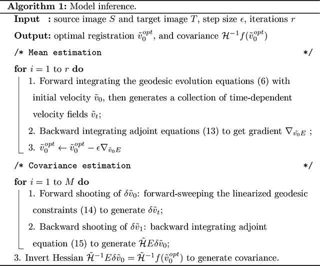
We summarize the inference of our algorithm in Alg. 1.

5. Results

To show the effectiveness of our model, we run experiments on both 2D synthetic data and 3D real brain MRI scans. We estimate the covariance by using α = 3, c = 6 for the operator $\tilde{L}$. We set band-limited dimension of the initial velocity field as 16, which is similar to the settings used in the pairwise diffeomorphic image registration [14]. We run both our model and baseline algorithms till convergence, with the number of time steps for Euler integration in geodesic shooting being 10.

Data

We simulate a collection of 2D synthetic dataset starting from a binary circle with resolution 100×100. We then generate smooth initial velocity fields from the prior distribution $p\left({\tilde{v}}_0\right)$, defined in Eq. (9). The deformed binary circles (used as our target images) are constructed by deforming the binary circle image with forward shooting the initial velocities.

The brain MRI scans of 60 subjects from the OASIS dataset [17], aged 60 to 90. All MRIs have the same resolution 128 × 128 × 128 with the voxel size of 1.25 × 1.25 × 1.25mm³. To further evaluate the accuracy of our mean estimation (registration solution), we use 10 pairs of 3D brain MRI scans with manual segmentation labels from public released ADNI dataset [28]. All images underwent the preprocessing of skull-stripping, downsampling, intensity normalization to [0,1] interval, bias field correction, and co-registration with affine transformations

Experiments

We first evaluate the proposed approach on 2D synthetic data and compare with the state-of-the-art diffeomorphic registration uncertainty quantification algorithm defined in a full-dimensional image space [15]. This baseline algorithm is defined in the original high-dimensional image space, where the full hessian is approximated via low-rank basis obtained by principal component analysis. The authors then compute the covariance matrix by inverting the approximated low-rank Hessian.

A visualization of uncertainty map estimated by the covariance matrix will be demonstrated. We set the initialization of initial velocity fields as zero and σ = 0.01 for both methods. We then validate our model on real 3D brain MRIs. Note that it is difficult to measure the accuracy of uncertainty methods since there is no registration ground truth exists. In order to demonstrate the effectiveness of our method in a statistical way, we report the difference between the Hessian without low-dimensional approximation and the Hessian estimated by our method both on 2D synthetic and 3D real data. In addition to estimate the final uncertainty maps, we show the time and memory comparison of all algorithms.

Finally, we demonstrate that another benefit of our model is the improved performance of mean estimation by standard image registration problem. Rather than finding an optimal registration result (mean) in a high-dimensional image space by using gradient descent algorithm, we instead perform an entire optimization in a low-dimensional bandlimited space. This not only makes the algorithmic inference much faster, but also reduces the risk of getting stuck in local minima. We compare our algorithm with the state-of-the-art fast diffeomorphic registration schemes: Quicksilver [29] and Voxelmorph [30]. To evaluate the estimated deformations, we perform registration-based segmentation and examine the resulting segmentation accuracy. The volume overlap, also known as Dice Similarity Coefficient (DSC), between the propagated segmentation A and the manual segmentation B for each structure is computed as (A, B) = 2(|A|∩|B|)/(|A|+|B|) where ∩ denotes an intersection of two regions.

Experimental results

Fig. 2 visualizes the uncertainty information estimated from both our method and the baseline algorithm performed in high-dimensional space on 2D data. We extract the local covariance matrix of each voxel and visualize it as an ellipse on the source image, with the color representing the matrix determinant. The smaller determinants are closer to the non-isotropic area (e.g., circle boundaries), which indicate more confident registration results.

Figure 2:

Left to right: source image, target image, covariance matrix determinant estimated by the baseline algorithm and our method.

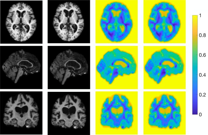
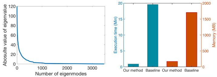
Fig. 3 visualizes an example of 3D brain registration uncertainty. Note that due to the difficulty of computing a full covariance matrix by inverse Hessian in a high dimensional image space, we need to use an approximated low-rank Hessian with a number of dominant eigenmodes [15]. Based on our key observation that the eigenvalues of Hessian matrix decay fast (as shown on the left panel of Fig. 4), we calculated the variances with various numbers of eigenmodes and noticed that the difference between covariances goes to zero beyond 2600 eigenmodes. Following [15], we then choose the first 2600 eigenmodes to approximate the full covariance accordingly. Both two methods show that the high uncertainty (with less confidence) appear isotropic areas (e.g., inside the ventricle), while the low uncertainty (with high confidence) appears around non-isotropic areas (e.g. ventricle boundaries). The right panel of Fig. 4 reports the comparison of time and memory consumption. Our algorithm offers significant improvements in computational efficiency. It is worth mentioning that while we adopted FLASH [14] for fast registration in our paper, the proposed Bayesian framework can be generalized to other registration models with the same level of efficiency, e.g., stationary velocity fields that remain constant over time [31], or projected subspace of velocity fields that characterizes deformations in a much lower dimensional space [32].

Figure 3:

Left to right: source image, target image, and uncertainty (visualized as the trace of covariance) estimated by baseline algorithm and our method.

Figure 4:

Left panel: eigenvalues of the Hessian matrix estimated by the baseline algorithm; Right panel: comparison of average runtime and memory consumption for all test cases.

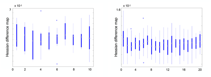
Fig. 5 reports the absolute value of difference between the Hessian estimated by our method and the full Hessian on ten pairs of 2D synthetic data and twenty pairs of 3D MRI scans. The low errors on both 2D and 3D experiments indicate that our estimation is fairly close to the optimal uncertainty result.

Figure 5:

Difference between the Hessian matrices estimated by our method and the full Hessian on both 2D and 3D data.

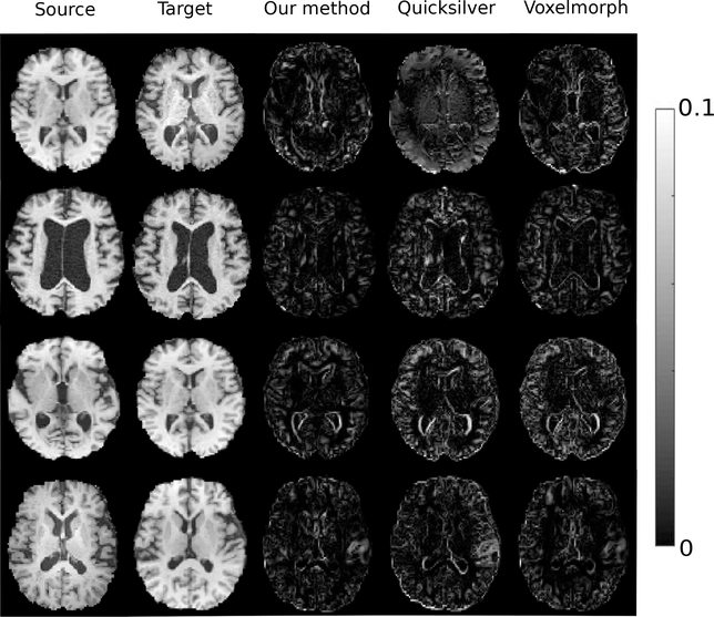
Fig. 6 displays example error maps between deformed source images by the estimated mean (an optimal of registration) from all methods and target images. It shows that our method achieves better registration results (a.k.a, smaller errors) than the two baseline algorithm [29, 30].

Figure 6:

Left to right: source image, target image, difference map of deformed image by estimated mean of our model, Quicksilver [29], and Voxelmorph [30].

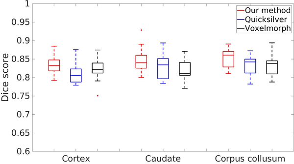
Fig. 7 reports the dice evaluations on brain cortex over 10 pairs of images for all methods. Our algorithm produces better dice score than the other two baseline algorithms.

Figure 7:

Dice score evaluated on the brain structure, cortex, caudate and corpus collusum of our method, Quicksilver, and Voxelmorph.

6. Conclusion

We presented a novel Bayesian model for registration uncertainty quantification in the space of diffeomorphic transformations. In contrast to previous approaches, our method significantly reduced the computational cost of the registration posterior inference effectively via (i) a low-dimensional representation of velocity fields that are associated with deformation fields; and (ii) an efficient Laplace’s approximation to the posterior distribution, where the covariance was fully estimated by second-order methods. This work is the first step toward efficient probabilistic models of registration uncertainty quantification based on high-dimensional geometric transformations. Our future work will be investigating sampling methods to thoroughly assess our developed model uncertainty, and further extending its application to real clinical settings, e.g., real-time image-guided navigation system for neurosurgery. While in this paper we focused on the representation of time-dependent velocity fields in the context of LDDMM, our method is general to other transformation parameterizations such as stationary velocity fields [31].

Appendix

This section includes the supplementary materials of computational derivatives for gradient term and second-order Hessian approximation.

Formulation of first derivative: gradient computation

As we derived in Sec. 2, the augmented energy with the adjoint variables ${\widehat{v}}_t$, ${\widehat{u}}_t$ can be formed as follows after adding geodesic constraints as Lagrangian multipliers,

$$\begin{gathered} \text{E}\left({\tilde{v}}_0\right)=-\ln p\left({\tilde{v}}_0|S,T,{\sigma }^2\right)+\underset{1}{\underbrace{{\int }_0^1\langle {\widehat{v}}_t,{\dot{\tilde{v}}}_t+{\mathrm{ad}}_{{\tilde{v}}_t}^{†}{\tilde{v}}_t\rangle }} \\ +\underset{2}{\underbrace{\langle {\widehat{u}}_t,{\dot{\tilde{u}}}_t+{\tilde{v}}_t+\tilde{\mathcal{D}}{\tilde{u}}_t\ast {\tilde{v}}_t\rangle dt}}. \end{gathered}$$ (16)

Next, we derive the variation of $\tilde{E}$ w.r.t the variables ${\tilde{v}}_0$ and ${\tilde{u}}_0$ for 1,2 respectively. To simplify the notation, we drop the subscript of time index t in the following sections.

Each part of the first derivative of ${\partial }_{\tilde{v}}E$ is,

$$1:{\frac{\partial }{\partial ϵ}|}_{ϵ=0}{\int }_0^1\langle \widehat{v},{\partial }_t(\tilde{v}+ϵ\delta \tilde{v})+{\mathrm{ad}}_{\tilde{v}+ϵ\delta \tilde{v}}^{†}(\tilde{v}+ϵ\delta \tilde{v})\rangle$$

$$2:{\frac{\partial }{\partial ϵ}|}_{ϵ=0}\left({\int }_0^1\langle \widehat{u},\tilde{v}+ϵ\delta \tilde{v}+\tilde{\mathcal{D}}\tilde{u}\ast (\tilde{v}+ϵ\delta \tilde{v})\rangle \right)$$

$$\begin{gathered} 1,2:{\int }_0^1\langle \widehat{v},\delta \dot{\tilde{v}}+{\mathrm{ad}}_{\tilde{v}}^{†}\delta \tilde{v}+{\mathrm{ad}}_{\delta \tilde{v}}^{†}\tilde{v}\rangle +{\int }_0^1\langle \widehat{u},\delta \tilde{v}+\tilde{\mathcal{D}}u\ast \delta \tilde{v}\rangle \\ ={\langle \widehat{v},\delta \tilde{v}\rangle |}_{t=0}^{t=1}-{\int }_0^1\langle \dot{\widehat{v}},\delta \tilde{v}\rangle +{\int }_0^1\langle {\text{ad}}_{\tilde{v}}\widehat{v}-{\mathrm{ad}}_{\widehat{v}}^{†}\tilde{v},\delta \tilde{v}\rangle \\ +{\int }_0^1\langle \widehat{u}+{(\tilde{\mathcal{D}}\tilde{u})}^T\star \widehat{u},\delta \tilde{v}\rangle \\ ={\langle \widehat{v},\delta \tilde{v}\rangle |}_{t=0}^{t=1}+{\int }_0^1\langle -\dot{\widehat{v}}+{\mathrm{ad}}_{\tilde{v}}\widehat{v}-{\mathrm{ad}}_{\widehat{v}}^{†}\tilde{v}+\widehat{u}+{(\tilde{\mathcal{D}}\tilde{u})}^T\star \widehat{u},\delta \tilde{v}\rangle . \end{gathered}$$ (17)

Each part of the first derivative ${\partial }_{\tilde{u}}E$ is

$$\begin{gathered} 1,2:{\partial }_{\tilde{u}}E={\frac{\partial }{\partial ϵ}|}_{ϵ=0}\left({\int }_0^1\langle \widehat{u},{\partial }_t(\tilde{u}+ϵ\delta \tilde{u})+\tilde{\mathcal{D}}(\tilde{u}+ϵ\delta \tilde{u})\ast \tilde{v}\rangle \right) \\ ={\int }_0^1\langle \widehat{u},\delta \dot{u}+\tilde{\mathcal{D}}\delta \tilde{u}\ast \tilde{u}\rangle \\ ={\langle \widehat{u},\delta \tilde{u}\rangle |}_{t=0}^{t=1}-{\int }_0^1\langle \dot{\widehat{u}},\delta \tilde{u}\rangle -{\int }_0^1\langle \delta \tilde{u},\tilde{\mathcal{D}}\tilde{u}\ast \tilde{v}+\tilde{u}\ast \tilde{\nabla }\cdot \tilde{v}\rangle \\ ={\langle \widehat{u},\delta \tilde{u}\rangle |}_{t=0}^{t=1}-{\int }_0^1\langle \delta \tilde{u},\dot{\widehat{u}}+\tilde{\mathcal{D}}\tilde{u}\ast \tilde{v}+\tilde{u}\ast \tilde{\nabla }\cdot \tilde{v})\rangle . \end{gathered}$$ (18)

By setting Eq. (18) to zero, we have ${\dot{\widehat{u}}}_t=-\tilde{\mathcal{D}}\delta {\widehat{u}}_t\ast {\tilde{v}}_t-\delta {\widehat{u}}_t\ast \left(\tilde{\nabla }\cdot {\tilde{v}}_t\right)$. Putting Eq. (17) and Eq. (18) together, we obtain the adjoint equations of Eq. (13),subject to initial conditions

$$\begin{gathered} {\widehat{v}}_1=0, \\ {\widehat{u}}_1=-\frac{1}{{\sigma }^2}\langle \nabla S_1,S_1-T\rangle . \end{gathered}$$

Formulation of second-order derivation: Hessian computation

We develop a similar forward-backward approach to compute the second derivatives of $\tilde{v}$ and $\tilde{u}$. We first derive the second-order forward shooting equation of by adding auxiliary variables $\delta \widehat{v}$ and $\delta \widehat{u}$ on the geodesic shooting EpDiff Eq. (6) and deformation transport equation Eq. (7) respectively.

For $\delta \tilde{v}$,

$$\begin{gathered} {\partial }_{\delta \tilde{v}}^{2}E={\frac{{\partial }^2}{\partial ϵ}|}_{ϵ=0}{\int }_0^1\langle \delta \widehat{v},{\partial }_t(\delta \tilde{v}+ϵ\delta \widehat{v})+{\mathrm{ad}}_{\tilde{v}+ϵ\delta \widehat{v}}^{†}(\tilde{v}+ϵ\delta \widehat{v})\rangle \\ ={\frac{\partial }{\partial ϵ}|}_{ϵ=0}{\int }_0^1\langle \delta \widehat{v},\delta \dot{\tilde{v}}+{\mathrm{ad}}_{\tilde{v}+ϵ\delta \widehat{v}}^{†}\delta \tilde{v}+{\mathrm{ad}}_{\delta \tilde{v}}^{†}(\tilde{v}+ϵ\delta \widehat{v})\rangle \\ +{\int }_0^1\langle \delta \widehat{v},{\partial }_t(\delta \widehat{v}+ϵ\delta \widehat{v})+{\mathrm{ad}}_{\tilde{v}+ϵ\delta \widehat{v}}^{†}(\tilde{v}+ϵ\delta \widehat{v})\rangle \\ ={\int }_0^1\langle \delta \widehat{v},\delta \dot{\tilde{v}}+{\mathrm{ad}}_{\tilde{v}}^{†}\delta \tilde{v}+{\mathrm{ad}}_{\delta \tilde{v}}^{†}\tilde{v}\rangle +\langle \delta \tilde{v},\dot{\tilde{v}}+{\mathrm{ad}}_{\tilde{v}}^{†}\tilde{v}\rangle . \end{gathered}$$ (19)

We then derive the forward shooting equation for $\delta \tilde{u}$ as follows,

$$\begin{gathered} {\partial }_{\delta \tilde{u}}E={\frac{{\partial }^2}{\partial ϵ}|}_{ϵ=0}{\int }_0^1\langle \delta \widehat{u},{\partial }_t(\tilde{u}+ϵ\delta \widehat{u})+\tilde{v}+ϵ\delta \widehat{v}+\tilde{\mathcal{D}}(\tilde{u}+ϵ\delta \widehat{u})\ast (\tilde{v}+ϵ\delta \widehat{v})\rangle \\ ={\frac{\partial }{\partial ϵ}|}_{ϵ=0}{\int }_0^1\langle \delta \widehat{u},\stackrel{.}{\delta \tilde{u}}+\delta \tilde{v}+\tilde{\mathcal{D}}\delta \tilde{u}\ast \tilde{v}+\tilde{\mathcal{D}}(\tilde{u}+ϵ\delta \widehat{u})\ast \delta \tilde{v}\rangle \\ +\langle \delta \widehat{u},{\partial }_t(\tilde{u}+ϵ\delta \widehat{u})+\tilde{v}+ϵ\delta \widehat{v}+\tilde{\mathcal{D}}(\tilde{u}+ϵ\delta \widehat{u})\ast (\tilde{v}+ϵ\delta \widehat{v})\rangle \\ ={\int }_0^1\langle \delta \widehat{u},\delta \dot{\tilde{u}}+\delta \tilde{v}+\tilde{\mathcal{D}}\delta \tilde{u}*\tilde{v}+\tilde{\mathcal{D}}\tilde{u}\ast \delta \tilde{v}\rangle +{\int }_0^1\langle \delta \widehat{u},\dot{\tilde{u}}+\tilde{v}+\tilde{\mathcal{D}}\tilde{u}\ast \tilde{v}\rangle . \end{gathered}$$ (20)

By setting Eq. (19) and Eq. (20) to zero, we obtain the second-order forward shooting for $\delta \tilde{v}$ and $\delta \tilde{u}$ as stated in Eq. (14).

Next we construct the augmented energy by adding second-order forward shooting equations as Lagrangian multipliers.

$$\begin{gathered} \text{E}\left(\delta {\widehat{v}}_0\right)=-\ln p\left({\widehat{v}}_0|S,T,{\sigma }^2\right) \\ +\underset{1}{\underbrace{{\int }_0^1\langle \delta \widehat{v},\delta \dot{\tilde{v}}+{\mathrm{ad}}_{\delta \tilde{v}}^{†}\tilde{v}+{\mathrm{ad}}_{\tilde{v}}^{†}\delta \tilde{v}\rangle }} \\ +\underset{2}{\underbrace{\langle \delta \widehat{u},\delta \dot{\tilde{u}}+\tilde{\mathcal{D}}\delta \tilde{u}\ast \tilde{v}-\tilde{\mathcal{D}}\tilde{u}\ast \delta \tilde{v}-\delta \tilde{v}\rangle }}. \end{gathered}$$

Similarly, we derive the second-order backward shooting equation by adding auxiliary variables $\delta \widehat{v}$ and $\delta \widehat{u}$ on part 1 and 2.

For $\delta \tilde{v}$,

$$\begin{gathered} {\partial }_{\delta \tilde{v}}^{2}E={\frac{\partial }{\partial ϵ}|}_{ϵ=0}{\int }_0^1\langle \delta \widehat{v},{\partial }_t(\delta \tilde{v}+ϵ\delta \widehat{v})+{\mathrm{ad}}_{\delta \tilde{v}+ϵ\delta \widehat{v}}\tilde{v}+{\mathrm{ad}}_{\tilde{v}}(\delta \tilde{v}+ϵ\delta \widehat{v})\rangle \\ +\langle \delta \widehat{u},\partial (\delta \tilde{v}+ϵ\delta \widehat{v})+\tilde{\mathcal{D}}\delta \tilde{u}\ast \tilde{v}+\tilde{\mathcal{D}}\tilde{u}\ast (\delta \tilde{v}+ϵ\widehat{v})+(\delta \tilde{v}+ϵ\delta \widehat{v})\rangle \\ ={\langle \delta \widehat{v},\delta \tilde{v}\rangle |}_{t=0}^{t=1}+{\int }_0^1\langle \delta \widehat{v},-\delta \dot{\tilde{v}}+{\mathrm{ad}}_{\tilde{v}}\delta \tilde{v}-{\mathrm{ad}}_{\delta \tilde{v}}^{†}\tilde{v}+\delta \tilde{u}+{(\tilde{\mathcal{D}}\tilde{u})}^T\star \delta \tilde{u}\rangle \\ +{\int }_0^1\langle \delta \widehat{v},-\delta \dot{\tilde{v}}+{\mathrm{ad}}_{\delta \tilde{v}}\tilde{v}-{\mathrm{ad}}_{\tilde{v}}^{†}\delta \tilde{v}+{(\tilde{\mathcal{D}}\delta \tilde{u})}^T\star \tilde{u}\rangle . \end{gathered}$$ (21)

For $\delta \tilde{u}$,

$$\begin{gathered} {\partial }_{\delta \tilde{u}}^{2}E={\frac{\partial }{\partial ϵ}|}_{ϵ=0}{\int }_0^1\langle \delta \widehat{u},{\partial }_t(\delta \tilde{u}+ϵ\delta \widehat{u})+{\mathrm{ad}}_{\delta \tilde{v}}\tilde{v}+{\mathrm{ad}}_{\tilde{v}}(\delta \tilde{v})\rangle \\ +\langle \delta \widehat{u},{\partial }_t(\delta \tilde{u}+ϵ\delta \widehat{u})+\tilde{\mathcal{D}}(\delta \tilde{u}+ϵ\delta \widehat{u})\ast \tilde{v}+\tilde{\mathcal{D}}\tilde{u}\ast \delta \tilde{v}-\delta \tilde{v}\rangle \\ ={\frac{\partial }{\partial ϵ}|}_{ϵ=0}{\int }_0^1\langle \delta \widehat{u},{\partial }_t(\delta \tilde{u}+ϵ\delta \widehat{u})+\tilde{\mathcal{D}}(\tilde{u}+ϵ\delta \widehat{u})\ast \tilde{v}\rangle \\ +\langle \delta \widehat{u},{\partial }_t(\delta \tilde{u}+ϵ\delta \widehat{u})+\tilde{\mathcal{D}}(\tilde{u}+ϵ\delta \widehat{u})\ast \delta \tilde{v}\rangle \\ ={\langle \delta \widehat{u},\delta \tilde{u}\rangle |}_{t=0}^{t=1}+{\int }_0^1\langle -\delta \widehat{u},\delta \dot{\tilde{u}}+\tilde{\mathcal{D}}\delta \tilde{u}\ast \tilde{v}+\delta \tilde{v}\ast \tilde{\nabla }\cdot \tilde{v}\rangle \\ +{\int }_0^1\langle -\delta \widehat{u},\stackrel{.}{\delta \tilde{u}}+\tilde{\mathcal{D}}\tilde{u}\ast \delta \tilde{v}+\tilde{u}\ast \tilde{\nabla }\cdot \delta \tilde{v}\rangle . \end{gathered}$$ (22)

By setting Eq. (21) and Eq. (22) to 0, we arrive the second-order backward equations of $\delta \tilde{v}$ and $\delta \tilde{u}$ as Eq. (15), subject to initial conditions $\delta {\widehat{u}}_1=-\frac{2}{{\sigma }^2}\mathcal{F}[\nabla S(1)\cdot \nabla S(1)+(S(1)-T)\cdot {\nabla }^{2}S(1)]$ and $\delta {\widehat{v}}_1=0$.

References

- [1].Christensen GE, Rabbitt RD, Miller MI, et al. , Deformable templates using large deformation kinematics, IEEE transactions on image processing 5 (10) (1996) 1435–1447. [DOI] [PubMed] [Google Scholar]
- [2].Christensen GE, Rabbitt RD, Miller MI, A deformable neuroanatomy textbook based on viscous fluid mechanics, in: 27th Ann. Conf. on Inf. Sciences and Systems, 1993, pp. 211–216. [Google Scholar]
- [3].Zhang M, Fletcher PT, Bayesian principal geodesic analysis in diffeomorphic image registration, in: International Conference on Medical Image Computing and Computer-Assisted Intervention, Springer, 2014, pp. 121–128. [DOI] [PubMed] [Google Scholar]
- [4].Zhang M, Fletcher PT, Bayesian principal geodesic analysis for estimating intrinsic diffeomorphic image variability, Medical image analysis 25 (1) (2015) 37–44. [DOI] [PubMed] [Google Scholar]
- [5].Ashburner J, Friston KJ, Unified segmentation, Neuroimage 26 (3) (2005) 839–851. [DOI] [PubMed] [Google Scholar]
- [6].Joshi S, Davis B, Jomier M, Gerig G, Unbiased diffeomorphic atlas construction for computational anatomy, NeuroImage 23 (2004) S151–S160. [DOI] [PubMed] [Google Scholar]
- [7].Risholm P, Pieper S, Samset E, Wells WM, Summarizing and visualizing uncertainty in non-rigid registration, in: International Conference on Medical Image Computing and Computer-Assisted Intervention, Springer, 2010, pp. 554–561. [DOI] [PMC free article] [PubMed] [Google Scholar]
- [8].Luo J, Toews M, Machado I, Frisken S, Zhang M, Preiswerk F, Sedghi A, Ding H, Pieper S, Golland P, et al. , A feature-driven active framework for ultrasound-based brain shift compensation, arXiv preprint arXiv:1803.07682. [Google Scholar]
- [9].Risholm P, Samset E, Wells W, Bayesian estimation of deformation and elastic parameters in non-rigid registration, in: International Workshop on Biomedical Image Registration, Springer, 2010, pp. 104–115. [Google Scholar]
- [10].Wassermann D, Toews M, Niethammer M, Wells W, Probabilistic diffeomorphic registration: Representing uncertainty, in: International Workshop on Biomedical Image Registration, Springer, 2014, pp. 72–82. [Google Scholar]
- [11].Kybic J, Bootstrap resampling for image registration uncertainty estimation without ground truth, IEEE Transactions on Image Processing 19 (1) (2010) 64–73. [DOI] [PubMed] [Google Scholar]
- [12].Le Folgoc L, Delingette H, Criminisi A, Ayache N, Quantifying registration uncertainty with sparse bayesian modelling, IEEE transactions on medical imaging 36 (2) (2017) 607–617. [DOI] [PubMed] [Google Scholar]
- [13].Zhang M, Fletcher PT, Finite-dimensional lie algebras for fast diffeomorphic image registration, in: International Conference on Information Processing in Medical Imaging, Springer, 2015, pp. 249–260. [DOI] [PubMed] [Google Scholar]
- [14].Zhang M, Liao R, Dalca AV, Turk EA, Luo J, Grant PE, Golland P, Frequency diffeomorphisms for efficient image registration, in: International Conference on Information Processing in Medical Imaging, Springer, 2017, pp. 559–570. [DOI] [PMC free article] [PubMed] [Google Scholar]
- [15].Yang X, Niethammer M, Uncertainty quantification for lddmm using a low-rank hessian approximation, in: International Conference on Medical Image Computing and Computer-Assisted Intervention, Springer, 2015, pp. 289–296. [Google Scholar]
- [16].Wang J, Wells WM, Golland P, Zhang M, Efficient laplace approximation for bayesian registration uncertainty quantification, in: International Conference on Medical Image Computing and Computer-Assisted Intervention, Springer, 2018, pp. 880–888. [DOI] [PMC free article] [PubMed] [Google Scholar]
- [17].Marcus DS, Wang TH, Parker J, Csernansky JG, Morris JC, Buckner RL, Cross-sectional mri data in young, middle aged, nondemented and demented older adults, Cognitive Neuroscie (2007) 1489–1507. [DOI] [PubMed] [Google Scholar]
- [18].Beg MF, Miller MI, Trouvé A, Younes L, Computing large deformation metric mappings via geodesic flows of diffeomorphisms, International journal of computer vision 61 (2) (2005) 139–157. [Google Scholar]
- [19].Zhang M, Fletcher PT, Fast diffeomorphic image registration via fourier-approximated lie algebras, International Journal of Computer Vision (2018) 1–13. [Google Scholar]
- [20].Vialard F-X, Risser L, Rueckert D, Cotter CJ, Diffeomorphic 3d image registration via geodesic shooting using an efficient adjoint calculation, International Journal of Computer Vision 97 (2) (2012) 229–241. [Google Scholar]
- [21].Avants BB, Epstein CL, Grossman M, Gee JC, Symmetric diffeomorphic image registration with cross-correlation: evaluating automated labeling of elderly and neurodegenerative brain, Medical image analysis 12 (1) (2008) 26–41. [DOI] [PMC free article] [PubMed] [Google Scholar]
- [22].Leventon M, Wells WM III, Grimson WEL, Multiple view 2d-3d mutual information registration, in: Image Understanding Workshop, Vol. 20, Citeseer, 1997, p. 21. [Google Scholar]
- [23].Arnol’d VI, Sur la géométrie différentielle des groupes de Lie de dimension infinie et ses applications à l’hydrodynamique des fluides parfaits, Ann. Inst. Fourier 16 (1966) 319–361. [Google Scholar]
- [24].Miller MI, Trouvé A, Younes L, Geodesic shooting for computational anatomy, Journal of Mathematical Imaging and Vision 24 (2) (2006) 209–228. doi: 10.1007/s10851-005-3624-0. [DOI] [PMC free article] [PubMed] [Google Scholar]
- [25].Zhang M, Singh N, Fletcher PT, Bayesian estimation of regularization and atlas building in diffeomorphic image registration, in: International conference on information processing in medical imaging, Springer, 2013, pp. 37–48. [DOI] [PMC free article] [PubMed] [Google Scholar]
- [26].Simpson IJ, Woolrich MW, Cardoso MJ, Cash DM, Modat M, Schnabel JA, Ourselin S, A bayesian approach for spatially adaptive regularisation in non-rigid registration, in: International Conference on Medical Image Computing and Computer-Assisted Intervention, Springer, 2013, pp. 10–18. [DOI] [PubMed] [Google Scholar]
- [27].Wong WH, Li B, Laplace expansion for posterior densities of nonlinear functions of parameters, Biometrika 79 (2) (1992) 393–398. [Google Scholar]
- [28].Jack CR Jr, Bernstein MA, Fox NC, Thompson P, Alexander G, Harvey D, Borowski B, Britson PJ, Whitwell JL, Ward C, et al. , The alzheimer’s disease neuroimaging initiative (adni): Mri methods, Journal of Magnetic Resonance Imaging: An Official Journal of the International Society for Magnetic Resonance in Medicine 27 (4) (2008) 685–691. [DOI] [PMC free article] [PubMed] [Google Scholar]
- [29].Yang X, Kwitt R, Styner M, Niethammer M, Quicksilver: Fast predictive image registration–a deep learning approach, NeuroImage 158 (2017) 378–396. [DOI] [PMC free article] [PubMed] [Google Scholar]
- [30].Balakrishnan G, Zhao A, Sabuncu MR, Guttag J, Dalca AV, An unsupervised learning model for deformable medical image registration, in: Proceedings of the IEEE Conference on Computer Vision and Pattern Recognition, 2018, pp. 9252–9260. [Google Scholar]
- [31].Arsigny V, Commowick O, Pennec X, Ayache N, A log-euclidean framework for statistics on diffeomorphisms, in: International Conference on Medical Image Computing and Computer-Assisted Intervention, Springer, 2006, pp. 924–931. [DOI] [PubMed] [Google Scholar]
- [32].Wang J, Xing W, Kirby RM, Zhang M, Data-driven model order reduction for diffeomorphic image registration, in: International conference on information processing in medical imaging, 2019. [Google Scholar]