Significance
Our justice system relies critically on the use of forensic science. More than a decade ago, a highly critical report raised significant concerns as to the reliability of many forensic techniques. These concerns persist today. Of particular concern to us is the use of photographic pattern analysis that attempts to identify an individual from purportedly distinct features. Such techniques have been used extensively in the courts over the past half century without, in our opinion, proper validation. We propose, therefore, that a large class of these forensic techniques should be subjected to rigorous analysis to determine their efficacy and appropriateness in the identification of individuals.
Keywords: criminal justice, forensic science, pattern analysis, forensic identification
Abstract
A 2009 report by the National Academy of Sciences was highly critical of many forensic practices. This report concluded that significant changes and advances were required to ensure the reliability across the forensic sciences. We examine the reliability of one such forensic technique used for identification based on purported distinct patterns on the seams of denim pants. Although first proposed more than 20 years ago, no thorough analysis of reliability or reproducibility of this forensic technique has previously been reported. We performed a detailed analysis of this forensic technique to determine its reliability and efficacy.
In 2005, the US Congress authorized the National Academy of Sciences (NAS) to conduct a study of forensic science. Formed in the fall of 2006, a committee of legal, technical, and policy experts was tasked with a broad mandate to assess the state of forensic science and make recommendations for improving the development and use of forensic techniques.
Published in 2009, the committee’s far-reaching 328-page report (1) called for a broad and deep restructuring of how forensic techniques are validated and applied and how forensic analysts are trained and accredited. One of the report’s key findings was that “[w]ith the exception of nuclear DNA analysis, however, no forensic method has been rigorously shown to have the capacity to consistently, and with a high degree of certainty, demonstrate a connection between evidence and a specific individual or source” (ref. 1, p. 7). The report argued that forensic practitioners too often offered evidence based on forensic techniques that had been shown to be invalid or unreliable and that many forensic examiners exaggerated their testimony, inflating the reliability of their methods and conclusions.
A decade after the report’s release, Judge Harry Edwards, cochair of the original committee, wrote “We are still struggling with the inability of courts to assess the efficacy of forensic evidence. When a forensic expert testifies about a method that has not been found to be valid and reliable, the expert does not know what he does not know and cannot explain the limits of the evidence. This is unacceptable” (ref. 2, p. 2).
Consistent with the NAS’s critique, a large body of research has demonstrated that human judgement can increase the risk of error in the assessment of forensic evidence. Various contextual and cognitive factors, for example, have been shown to influence pattern comparison judgements in the analysis of fingerprint (3–5), hair (6), bite mark (7, 8), bloodstain (9), handwriting (10, 11), firearm ballistics (12, 13), and mixture DNA (14). Adding further concern, forensic analysts are often unable to accurately estimate the error rate associated with their specific technique (15). As noted by the NAS report, these errors can have severe consequences in the real world—the National Registry of Exonerations (http://www.law.umich.edu/special/exoneration) identified that flawed or misleading evidence gathered using forensic techniques contributed to almost a quarter of wrongful convictions in the United States between 1989 and 2019. It is, therefore, apparent that more research is required to examine the reliability of human assessment of forensic evidence. A useful framework for this examination is the Hierarchy of Expert Performance (HEP), which identifies eight levels of performance that should be tested for each type of forensic technique (16).
A 2019 ProPublica article (17) drew attention to a particular category of forensic science termed photographic pattern analysis. Photographic examiners at the Federal Bureau of Investigation (FBI) Laboratory in Quantico routinely analyze crime scene photos to determine if certain details, such as features on a perpetrator’s face, hands, or clothing, match a suspect. When conducting their analysis, these examiners typically take a subjective approach often with a lack of objective criteria for defining pattern similarity, leading to inconsistency and potential bias (18–20). Such photographic comparisons are common, having been used to tie defendants to crime scenes in thousands of cases over the past 50 years. Although it is not known precisely how often photographic comparisons serve as central evidence in cases, FBI examiners have stated that they analyze photos in hundreds of cases each year.
As reported by ProPublica (17), this type of photographic pattern analysis served as central evidence in James D’Ambrosio’s bank robbery conviction in 1992. An FBI examiner analyzed surveillance images of the robbery and testified that the similarities in the wear marks along the seams of the jeans worn by the perpetrator matched those of a pair of jeans found in the defendant’s possession. This denim jean identification was also used in 1997 to identify suspects in a series of violent crimes in Washington State. An FBI examiner compared surveillance footage to a number of pairs of jeans seized from the suspects’ homes. This analysis led to the conclusion that a pair of jeans found at a suspect’s home matched a pair worn by one of the attackers.
This denim jean identification was described in a technical paper published in 1999 in which the author, then and still an FBI examiner, described a photographic pattern analysis for identifying denim jeans from purportedly distinct characteristics along the seams that result from the manufacturing process and subsequent wear-and-tear (21). Although the report describes the use of this technique as part of the identification of a suspect in the Washington State crime spree, the report also states “Although a validation study has yet to be performed to test the theory that all denim trouser barcode seam patterns are unique, it has been observed in numerous examinations that it is possible to distinguish pairs of jeans from one another based solely on differences in the patterns along the seams” (ref. 21, p. 615). The author concludes, however, that “A determination of whether individual characteristics like the ones discussed herein are unique or not will remain unanswered until validation studies can be conducted. Until that time, the ability to individualize an item based on a single such characteristic will remain a matter of opinion” (ref. 21, p. 621).
To our knowledge, however, in the intervening two decades, no thorough analysis of reliability or reproducibility of this forensic technique has previously been reported.
This 1999 publication (21), nonetheless has been cited as evidence that the method for denim jean identification meets the Daubert standard* and has also been used to substantiate the admission of other photographic pattern analyses. In 2002, for example, the central piece of evidence against Wilbert McKreith, charged with eight bank robberies, was a purported unique match between his plaid shirt and a shirt seen in surveillance footage. In this case, the FBI examiner claimed to have matched lines in the plaid pattern and went on to estimate the probability of this match occurring randomly to be 1-in-650 billion (see ref. 22 for a general description of the flaws in the statistical reasoning as used by the FBI examiner). In presenting this photographic pattern analysis, the FBI examiner cited the earlier denim jean publication (21) to establish the method as scientifically valid and therefore admissible.
Given the significance of the original denim jean analysis as a forensic technique accepted by the courts, and as a precedent for the introduction of other photographic pattern-matching techniques, it is critical that we better understand this forensic technique. We describe a detailed analysis of the reliability and reproducibility of identification based on the pattern of wear-and-tear along denim jeans.
Results
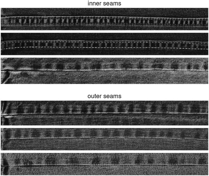
We collected images of 211 pairs of denim jeans (see representative examples in Fig. 1) and extracted a 1D pattern of wear and tear along the vertical left and right, inner and outer seams (Materials and Methods). We describe the distinctiveness of these patterns between different denim jeans and the reproducibility of these patterns within multiple images of the same pair of denim jeans. These two measurements are combined to provide expected false alarm rates (incorrectly matching two distinct seams) based on the seam pattern of wear and tear.
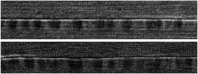
Fig. 1.
Three representative (Top) inner and (Bottom) outer seams.
Distinctiveness.
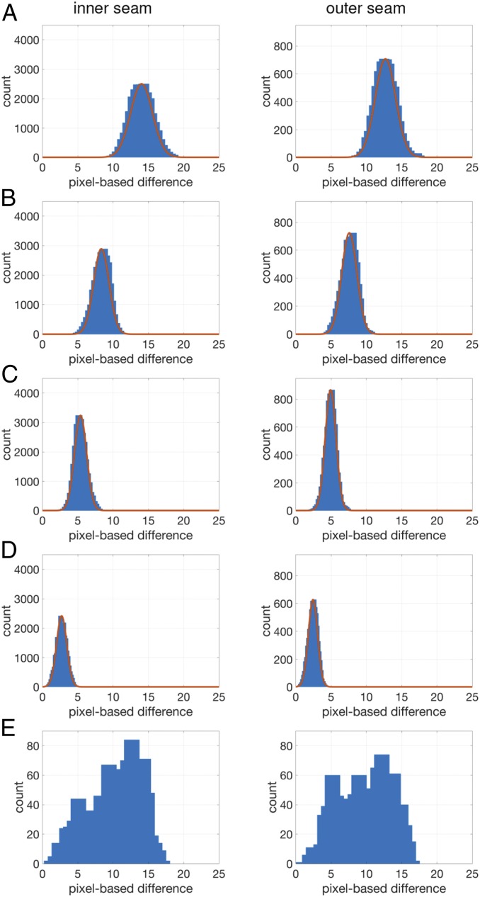
Shown in Fig. 2 A–D is the distribution of the minimum pixel-based differences† between different pairs of denim jeans for the inner and outer seams of varying length (24, 16, 12, and 8 cm). These distributions are collapsed across the left and right seams because the individual mean and standard deviations for the left and right seams are nearly indistinguishable (Table 1).
Fig. 2.
The distribution of minimum pixel-based difference between the inner and outer seams of length (A) 24, (B) 16, (C) 12, and (D) 8 cm between different pairs of denim pants (collapsed over left/right seams). The red curve is a fitted Gaussian distribution. See also Table 1. (E) The distributions for the inner and outer seams of length 24 cm between multiple images of the same pairs of denim jeans (collapsed, again, over left/right seams).
Table 1.
The mean (SD) pixel-based minimum (min) and median (med) difference between the left (L), right (R), and combined (L + R) and for the inner and outer seams of length between 24, 16, 12, and 8 cm between different pairs of denim pants
| Seam Length | ||||
| 24 cm | 16 cm | 12 cm | 8 cm | |
| Inner seam | ||||
| L (min) | 14.0 (1.56) | 8.3 (1.10) | 5.4 (0.87) | 2.7 (0.73) |
| R (min) | 14.1 (1.55) | 8.4 (1.08) | 5.4 (0.86) | 2.7 (0.72) |
| L + R (min) | 14.0 (1.56) | 8.3 (1.09) | 5.4 (0.86) | 2.7 (0.73) |
| L + R (med) | 17.7 (1.12) | 11.3 (0.63) | 8.6 (0.49) | 5.4 (0.31) |
| Outer seam | ||||
| L (min) | 12.8 (1.53) | 7.7 (1.11) | 5.0 (0.80) | 2.5 (0.68) |
| R (min) | 12.6 (1.39) | 7.5 (1.05) | 4.9 (0.75) | 2.4 (0.64) |
| L + R (min) | 12.7 (1.45) | 7.6 (1.08) | 4.9 (0.78) | 2.4 (0.66) |
| L + R (med) | 15.6 (1.43) | 10.1 (0.77) | 7.6 (0.72) | 4.8 (0.39) |
See also Fig. 2 A–D.
The average difference for inner seams of length 24 cm, for example, is 14.0, which should be interpreted to mean that on average, two different seams have matching ridges (bright regions along the seam) and valleys (dark regions along the seam) that are within 14 pixels and have at most 14 unmatched ridges and valleys. With an average difference of 12.7, outer seams of length 24 cm are slightly less distinct. As expected, the difference decreases as the seam length decreases from 24 to 8 cm.
The minimum difference, of course, represents the best match between two different seams. To ensure that this measure is not providing a biased representation of the overall distribution, we also report the median pixel-based differences in Table 1. Across both seams and all seam lengths, the median difference is, on average, only 2.9 units larger than the average minimum difference. This suggests that the minimum difference is not the result of an anomalous and nonrepresentative match.
We must now ask whether these differences are sufficient to support identification. To this end, we next report on the reproducibility between different analysts analyzing the same image, and the reproducibility of an analyst analyzing different images of the same pair of jeans.
Analyst Reproducibility.
To examine reproducibility across analysts, we report on the differences in analyzing the same images of denim jeans analyzed by two analysts (the authors). We selected 10 pairs of jeans for which all four seams passed the criteria for analysis (Materials and Methods). Two analysts performed their analyses independently. The average differences between the 24-cm inner and outer seams (averaged across left/right) between the analysts are 2.8 and 3.4, with SDs of 1.21 and 1.62. This difference is significantly smaller than the pixel-based differences seen in the previous section, suggesting that the underlying extraction and comparison is reliable.
To examine reproducibility within an analyst, one of the authors reanalyzed 10 pairs of jeans at two different times (with ∼6 mo between the first and second analyses). The average intraanalyst differences for the 24-cm inner and outer seams are 1.5 and 1.6, with SDs of 0.72 and 1.09. These small differences over time further suggest that the extraction and comparison method is reliable.
Pattern Reproducibility.
Starting with the same 10 pairs of jeans described in the previous section, each of the four seams was reimaged 10 additional times, each under varying conditions including different lighting, two different cameras, different surfaces onto which the jeans were placed, and different ways in which the material naturally and randomly draped.
Shown in Fig. 2E is the distribution of minimum pixel-based differences between all 11 versions of the same pair of pants collapsed, as before, across the left and right seams of length 24 cm. These distributions are generated from 1,100 difference measurements per inner/outer seam (55 comparisons per left/right and inner/outer seam, collapsed over left/right to yield 110 per inner/outer seam, times 10 different pairs of jeans). The inner and outer distributions have median differences of 10.7 and 10.0.
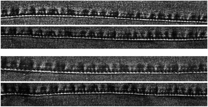
These somewhat bimodal distributions are clearly different from the distributions for seams from different jeans (Fig. 2A). Shown in Fig. 3 is an example of the variability of the difference from the same seams. In Fig. 3, each panel is of the same right-inner seam, but the difference of the top two seams is 6.5, while the difference of the bottom two seams is nearly two and half times larger at 15.9.
Fig. 3.
The identical right-inner seam imaged four different times. The minimum pixel-based difference for the top two seams is 6.5, and the difference for the bottom two seams is 15.9.
The bimodality in these distributions is not due to some jeans having high reproducibility and others having low reproducibility, because the same bimodality is seen for each pair of jeans. Instead, we hypothesize that the nonrigid nature of the material led to the distortions in the appearance of the seams and, in turn, the wide variability in their appearance.
We next combine the distributions in Fig. 2 A and E to determine the trade-off between accurately identifying the same seam pattern (true positive) and incorrectly matching two different seams (false positive).
Accuracy.
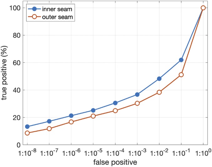
Shown in Fig. 4 is the true positive rate (correctly matching the same seams) as a function of the false positive rate (incorrectly matching different seams) for inner and outer seams of length 24 cm.
Fig. 4.
The true positive rate as a function of false positive rate (on a logarithmic scale) for inner (filled blue) and outer (open red) seams of length 24 cm. With a false positive of one in a million (), for example, the true positive rate is for inner seams and for outer seams.
Because of the limited data in the distributions in Fig. 2A, we used a fitted Gaussian to these distributions to allow us to estimate the false positive rate as low as 1 in 100 million (). Because the data in Fig. 2E are not normally distributed, the true positive rate was estimated directly from the data.
Without stating what false positive rate is acceptable, we note that the true positive rate falls rapidly as the false positive decreases. For the longest seam of 24 cm, the true positive rate for both the inner and outer seams is below at the relatively high false positive rate of one in a thousand (). At a false positive rate of one in a thousand, the true positive rate for the inner/outer seams of length 16, 12, and 8 cm, are , , and . The slight improvement for shorter seams is most likely due to the fact that any distortion in the material has less of an impact on shorter seams. Across all seams and seam lengths, however, the true positive rate is below for a false positive rate of one in a hundred thousand () and lower.
Shown in Fig. 5 is a pair of 24 cm left-outer seams from different pairs of pants having a pixel-based difference of 7.7, less than the median difference of 10.0 for the same pairs of pants (Fig. 2E). In addition to the low numeric difference, the seams are also visually similar. This is particularly striking given that these two similar seams are found from only a relatively small number of 81 left-outer seams in our dataset (Materials and Methods).
Fig. 5.
Two different but highly similar 24-cm left-outer seams with a pixel-based difference 7.7 (see, by comparison, Fig. 2).
Independence.
We have shown the trade-off between true positive and false positive for matching a single seam. If the differences between, for example, the left-inner and right-inner seams are independent, then it would be possible to combine multiple seam analyses to improve overall accuracy. This, of course, requires that the differences across these seams be independent.
To determine whether the differences of any two seams (left/right and inner/outer) are independent, we measured the correlation between the pairwise differences of all pairs of seams (Table 2). Shown in this table is the correlation coefficient () and the number of pairwise differences (). The correlations for the left-inner to right-inner and left-outer to right-outer are 0.46 and 0.52, revealing that these pairwise differences are not independent and should not be simply combined. On the other hand, the remaining four pairwise seams, between an inner and outer seam, with correlations between 0.11 and 0.18 reveal that these are relatively independent, suggesting that accuracy may be improved by combining across these seams.
Table 2.
The correlation coefficient () between the pairwise difference between two seams
| Seams | |||
| Left inner: right inner | 0.46 | 0.21 | 11,781 |
| Left outer: right outer | 0.52 | 0.28 | 1,653 |
| Left inner: left outer | 0.16 | 0.02 | 3,003 |
| Left inner: right outer | 0.16 | 0.03 | 3,570 |
| Left outer: right inner | 0.11 | 0.12 | 3,003 |
| Right inner: right outer | 0.18 | 0.03 | 3,486 |
All correlations are significant with .
Features.
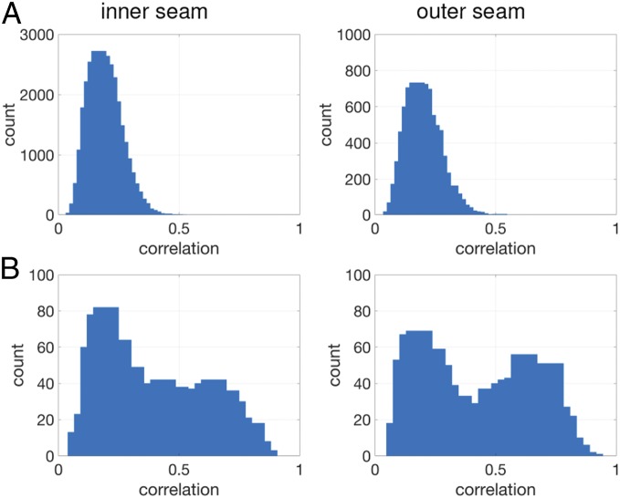
Although the reduction of the original seam pattern to discrete ridges and valleys was modeled after the original technique (21), it could be argued that this simplification eliminates a large amount of identifiable information. We, therefore, analyzed the full seam pattern (the low-pass filtered version; Fig. 7D) to determine if it provides a more distinct pattern for identification. In this analysis we compare the difference between two signals using a standard correlation coefficient.
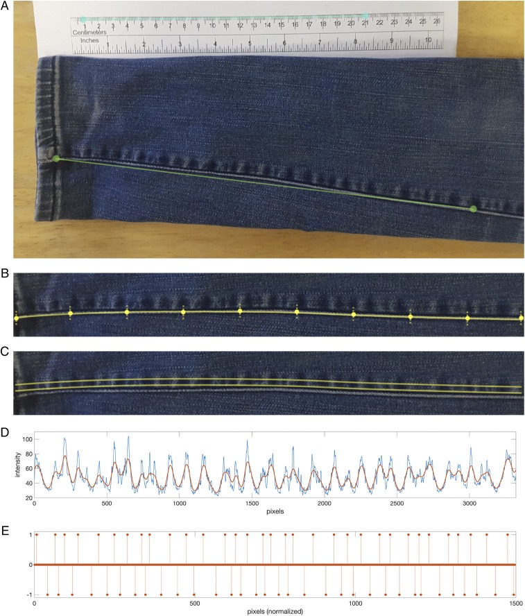
Fig. 7.
(A) An inner seam photographed with a calibration ruler, with the green line corresponding to an analyst’s selection of 30 cm along the seam. (B) The cropped and rotated seam from A annotated with 10 equally spaced points along the seam and a fitted 5-point Bezier curve. (C) Two Bezier curves offset by 30 pixels manually adjusted to select the seam pattern. (D) The intensity profile (blue) averaged over 30 curves bounded by the upper and lower curves shown in C. The signal in red corresponds to a low-passed version of this profile. (E) The low-pass signal normalized to a length of 1,500 pixels and converted to identify the ridges (with a value of 1) and valleys (with a value of ).
Shown in Fig. 6 is the distribution of the correlations between different (Fig. 6A) and same (Fig. 6B) pairs of denim jeans for the inner and outer seams of length 24 cm. As in Fig. 2 A and E, there is a large overlap between these distributions suggesting that even the full signal does not contain any more identifiable information than only the ridges and valleys.
Fig. 6.
The distribution of correlations between the inner and outer seams (collapsed over left/right seams) of length 24 cm between (A) different pairs of denim pants and (B) same pairs of denim pants.
Discussion
We have shown that the pattern of wear and tear on the seams of denim jeans is not as distinct as previously argued and is highly variable due—we posit—to the inherent nonrigidity of the denim material. Even under the nearly ideal imaging conditions of our analysis—a controlled and consistent setting and well-illuminated, high-resolution, and high-quality images—a combination of the lack of distinctiveness across jeans and the lack of consistency within jeans leads us to conclude that identification based on denim jeans should be used with extreme caution, if at all.
In particular, as shown in Fig. 4, with a false alarm of 1 in (), correct identification—again, under ideal imaging conditions—is expected to be ∼. This low identification rate raises significant concerns as to the usefulness of this photographic pattern analysis.
In addition, it is reasonable to expect that the reliability of this technique may degrade under real-world imaging conditions with low light, low signal-to-noise ratio, low resolution, perspective distortion, and material distortions that naturally arise when jeans are worn, as opposed to flattened out on a rigid surface, as was the case in our evaluation.
It may be the case that the reliability of this technique would improve with additional information like the jean brand and size along with other identifying marks like rips and tears, as well as other items of clothing (21, 23). Without a large-scale evaluation, however, it is impossible to determine if this is the case.
A critical component of the FBI photographic analysis unit is identifying individuals from surveillance footage. Because perpetrators of a crime are often masked, this identification cannot always be done with standard facial recognition. Instead, analysts examine other potentially identifying features such as clothing and distinctive markings on, for example, a hand. Given our results on the lack of distinctiveness of the pattern on denim jeans, it is natural to consider whether other forensic identification techniques suffer from the same accuracy and reproducibility problem.
When, for example, an FBI analyst identified the plaid shirt in a surveillance video as that belonging to Wilbert McKreith, the analyst stated in court that the odds that two different shirts would match were a staggering 1-in-650 billion. The analyst arrived at this number by making eight measurements along two seams, estimating the probability that the plaid stripes at these eight locations were misaligned by a certain distance, and then multiplying all eight of these probabilities to reach the astronomically low odds of 1-in-650 billion. This calculation is problematic for at least two reasons: 1) the initial probability of misalignment was based on an estimate of the distance between two plaid stripes and an estimate of the reliable resolution at which this distance can be reliably resolved, neither of which was based on a careful or detailed analysis, and 2) since the misalignment of multiple plaid stripes along the front and back of the shirt are obviously not independent, they cannot simply be combined. As with the denim jean analysis, a large-scale study is required to understand when and if this type of plaid shirt analysis should be used to identify individuals.
In 2015, Steve Talley was wrongly charged with aggravated bank robbery based on an FBI analyst’s comparison of facial markings (24). The FBI teaches that facial and body markings like freckles and moles can be used to reliably identify a person (17) (https://www.nist.gov/system/files/documents/2016/12/12/vorderbruegge-face.pdf). This analysis is problematic for at least two reasons: 1) no large-scale study has shown the distinctiveness of such facial and body markings and 2) no large-scale study has shown whether analysts can consistently identify the same markings in a photo [in fact, an FBI analyst has stated that reproducibility of identifying facial markings over time is not reliable (25)].
Purportedly distinct markings on denim jeans, plaid shirts, hands, and faces have been used to identify individuals from surveillance footage. Mistakes in these identifications are costly, resulting in an innocent person being accused or sentenced and a guilty person walking free. We advocate that any and all forensic photographic pattern analysis be subjected to the same type of rigorous analysis carried out here (26). We also advocate that these studies be carried out by independent groups and not the institutions that have previously been tasked with performing these forensic examinations.
Materials and Methods
This section describes the acquisition of a set of 211 denim jeans, the processing steps to extract the pattern along the denim seam, and a measure of difference for comparing two such seams. We note that the original description of the denim seam matching (21) employs an entirely manual analysis. We describe a more automated technique that attempts to remove as much subjectivity as possible from this analysis.
Dataset.
We collected four images of the left/right and inner/outer seams from each of 211 pairs of denim jeans. A total of 111 of these jeans were collected from workers on Amazon’s Mechanical Turk (AMT), and we purchased the remaining 100 pairs from two local used clothing shops.‡
The AMT workers were instructed to photograph the left/right and inner/outer seams for one pair of their denim jeans. They were instructed to lie the jeans along a well-lit, hard, flat surface with the seam running along the middle. They were also instructed to place a printed ruler, which we provided, alongside the jeans (Fig. 7) (this ruler allowed us to determine the pixel to cm conversion in each image). We asked workers to photograph at a minimum resolution of 6 megapixels (∼ pixels); any images below this resolution were excluded. We photographed our purchased jeans following the same instructions.
Although the seam along the bottom cuff was visible in all images, we excluded this seam from analysis because we found the material was often torn, dirty, distorted, and too small to yield reliable patterns.
Image Analysis.
An analyst (one of the authors) extracted the left/right and inner/outer seams from each image as follows. The image was first converted from color (RGB) to grayscale using a standard conversion: gray = 0.2989R + 0.5870G + 0.1140B. The analyst extracted a rectangular region of interest (ROI) that generously included the full width of the seam and a length of 30 cm starting just above the bottom cuff and extending upward toward the knee. For an average height person, this corresponds to the segment of leg from the cuff to slightly below the knee.
The ROI was selected by first manually selecting a point where the vertical seam intersects the cuff and then selecting a point 30 cm along the seam (Fig. 7A). These two reference points were used to orient the ROI so that the seam was oriented along the image’s horizontal axis.
The analyst then manually annotated equally spaced points along the length of the often curvy seam. A point Bezier curve (27) was then fit to these points (Fig. 7B). In particular, denote , as the user-selected points. The jth sampled Bezier basis function, , is given by the -D column vector:
| [1] |
where the vector exponentiation is point-wise and the -D vector consists of an equally sampled unit interval,
| [2] |
The Bezier control points are computed using least-squares estimation:
| [3] |
where the matrix is given by
| [4] |
and the matrix , consisting of the user-selected points, is given by
| [5] |
Each row of the matrix corresponds to the 2D spatial coordinates of one of Bezier control points. The parametric variable controls the spatial position along the Bezier curve, with one end of the Bezier corresponding to and the other end corresponding to . The spatial coordinates along any intermediate point on the curve at is given by
| [6] |
where is the Bezier control-point matrix (Eq. 3) and is a -D column vector whose jth component, , is
| [7] |
Two versions of a densely sampled Bezier curve, vertically offset by 30 pixels, were then manually adjusted to encompass the central part of the seam (Fig. 7C) . The underlying pixel intensity values along each of the 30 curves were determined using bicubic interpolation and averaged to yield a single 1D signal corresponding to the change in intensity along the seam (Fig. 7D). This averaging afforded some robustness to image noise and small variations in the denim pattern.
The analyst excluded any seams that did not satisfy each of the following properties: 1) the length of the seam was at least 30 cm, 2) the resolution of this 30-cm seam was at least 1,500 pixels, 3) the width of the seam was at least 30 pixels, and 4) the final extracted 1D signal clearly showed a distinct pattern of ridges and valleys. Because of the subjective nature of this last criterion, a second analyst (also an author) reviewed all decisions until a consensus across analysts was reached.
Enforcement of these criteria reduced the original 211 left/right and inner/outer seams to 164 left/inner, 162 right/inner, 81 left/outer, and 90 right/outer seams. The pattern along the outer seams was generally not as salient leading to considerably larger exclusion.
Signal Analysis.
Each 1D signal corresponding to a left/right and inner/outer seam is subjected to three preprocessing steps: 1) to eliminate small fluctuations in pixel intensity, the signal of length () is low-pass filtered by multiplying the signal’s -point Fourier transform with a Gaussian () (Fig. 7D); 2) the signal is normalized to a fixed resolution of 1,500 pixels; and 3) the ridges and valleys are then automatically extracted by identifying samples with a zero first-derivative and positive second-derivative (ridge) or a zero first-derivative and negative second-derivative (valley). The final 1D signal consists of samples with a value of 1 (ridge), (valley), and 0 otherwise (Fig. 7E).
We next describe a technique for quantifying the difference between two processed signals. Because these signals are non-Gaussian, we choose not to use the standard correlation measure of similarity. Instead, we leverage a technique from neural spike-train analysis that is designed to analyze similar types of signals (28). In particular, the difference between two spike-trains and is measured as the amount that a spike in must be moved to align with the corresponding spike in and the number of spikes that must be added or removed from in order to match . In our case, we compute this difference separately for the ridges (with a value of in Fig. 7E) and the valleys (with a value of in Fig. 7E) and sum these differences. The cost of moving and adding/deleting is controlled by a single parameter which we set to 0.1 throughout.
The difference between two corresponding seams (left/right and inner/outer) is given by the minimum segment length (of length ) along the entire seam.
The difference of a segment and , each of length , is computed as follows. The signal is aligned at the same distance from the bottom cuff as . The signal is then shifted by pixels in either direction of this alignment. The minimum difference across these 51 possible alignments is taken to be the measure of difference between and . This shifting is done to allow for slight misalignments between and . Next, the difference between the entire length of the seam is taken as the minimum segment difference along all shifted, by 50 pixels, segments along the seam.
Spike- to Pixel-Based Difference.
Although the spike-based measure of difference is effective, it does not provide an intuitive measure of difference. To this end, we convert the spike-based measurement to a more intuitive pixel-based measurement.
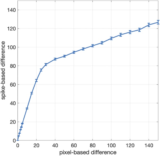
Starting with each of the 497 left/right and inner/outer seams, we synthetically generated perturbed versions of the 1D processed signals as follows: 1) the locations of the ridges and valleys were shifted by a random number of pixels in the range , 2) a random number in the range of ridges was added, and 3) a random number in the range of valleys was added (for a maximum of additional ridges and valleys). The segment difference (as defined above) between the original and perturbed signal was then computed. Shown in Fig. 8 is the mapping between the original spike difference and our pixel-based difference. With this measure, a pixel-based difference of corresponds to a maximum spatial offset between matching ridges and valleys of pixels and a maximum of missing or additional ridges/valleys.
Fig. 8.
Conversion from spike-based to pixel-based difference. The error bars correspond to confidence intervals.
Acknowledgments
We thank Marty Banks and Emily Cooper for their insights and many helpful discussions.
Footnotes
The authors declare no competing interest.
This article is a PNAS Direct Submission.
*Under the Daubert standard, judges assess the admissibility of expert witness testimony against a number of criteria to ensure that scientific testimony is based on scientifically valid and reliable methods. The Daubert standard, used in federal and many state courts, originates from the 1993 ruling in the US Supreme Court case Daubert v Merrell Dow Pharmaceuticals.
†As described in Materials and Methods, a pixel-based difference of corresponds to a maximum spatial offset between matching ridges and valleys of pixels and a maximum of missing or additional ridges/valleys.
‡All images are available for download on Figshare at https://figshare.com/articles/blueJeans-PNAS2020/11775126.
Data deposition: Supplementary data are available on Figshare (https://figshare.com/articles/blueJeans-PNAS2020/11775126).
References
- 1.Committee on Identifying the Needs of the Forensic Sciences Community, National Research Council , Strengthening Forensic Science in the United States: A Path Forward (National Academies Press, 2009). [Google Scholar]
- 2.Edwards H. T., Ten years after the National Academy of Sciences’ landmark report on strengthening forensic science in the United States: A path forward—Where are we? (New York University School of Law, New York, NY, 2019), Public Law Research Paper No. 19-23.
- 3.Ulery B. T., Hicklin R. A., Buscaglia J., Roberts M. A., Accuracy and reliability of forensic latent fingerprint decisions. Proc. Natl. Acad. Sci. U.S.A. 108, 7733–7738 (2011). [DOI] [PMC free article] [PubMed] [Google Scholar]
- 4.Dror I. E., Charlton D., Péron A. E., Contextual information renders experts vulnerable to making erroneous identifications. Forensic Sci. Int. 156, 74–78 (2006). [DOI] [PubMed] [Google Scholar]
- 5.et al. , Cognitive issues in fingerprint analysis: Inter-and intra-expert consistency and the effect of a ‘target’ comparison. Forensic Sci. Int. 208, 10–17 (2011). [DOI] [PubMed] [Google Scholar]
- 6.Miller L. S., Procedural bias in forensic science examinations of human hair. Law Hum. Behav. 11, 157–163 (1987). [Google Scholar]
- 7.Page M., Taylor J., Blenkin M., Context effects and observer bias–implications for forensic odontology. J. Forensic Sci. 57, 108–112 (2012). [DOI] [PubMed] [Google Scholar]
- 8.Osborne N. K., Woods S., Kieser J., Zajac R., Does contextual information bias bitemark comparisons? Sci. Justice 54, 267–273 (2014). [DOI] [PubMed] [Google Scholar]
- 9.Taylor M. C., Laber T. L., Kish P. E., Owens G., Osborne N. K., The reliability of pattern classification in bloodstain pattern analysis, part 1: Bloodstain patterns on rigid non-absorbent surfaces. J. Forensic Sci. 61, 922–927 (2016). [DOI] [PubMed] [Google Scholar]
- 10.Found B., Ganas J., The management of domain irrelevant context information in forensic handwriting examination casework. Sci. Justice 53, 154–158 (2013). [DOI] [PubMed] [Google Scholar]
- 11.Kukucka J., Kassin S. M., Do confessions taint perceptions of handwriting evidence? An empirical test of the forensic confirmation bias. Law Hum. Behav. 38, 256–270 (2014). [DOI] [PubMed] [Google Scholar]
- 12.Mattijssen E., Kerkhoff W., Berger C., Dror I., Stoel R., Implementing context information management in forensic casework: Minimizing contextual bias in firearms examination. Sci. Justice 56, 113–122 (2016). [DOI] [PubMed] [Google Scholar]
- 13.Kerkhoff W., et al. , Design and results of an exploratory double blind testing program in firearms examination. Sci. Justice 55, 514–519 (2015). [DOI] [PubMed] [Google Scholar]
- 14.Dror I. E., Hampikian G., Subjectivity and bias in forensic DNA mixture interpretation. Sci. Justice 51, 204–208 (2011). [DOI] [PubMed] [Google Scholar]
- 15.Murrie D. C., Gardner B. O., Kelley S., Dror I. E., Perceptions and estimates of error rates in forensic science: A survey of forensic analysts. Forensic Sci. Int. 302, 109887 (2019). [DOI] [PubMed] [Google Scholar]
- 16.Dror I. E., A hierarchy of expert performance. J. Appl. Res. Mem. Cognit. 5, 121–127 (2016). [Google Scholar]
- 17.Gabrielson R., The FBI says its photo analysis is scientific evidence. Scientists disagree. https://www.propublica.org/article/with-photo-analysis-fbi-lab-continues-shaky-forensic-science-practices. Accessed 30 January 2020.
- 18.Carriquiry A., Hofmann H., Tai X. H., VanderPlas S., Machine learning in forensic applications. Significance 16, 29–35 (2019). [Google Scholar]
- 19.Kassin S. M., Dror I. E., Kukucka J., The forensic confirmation bias: Problems, perspectives, and proposed solutions. J. Appl. Res. Mem. Cognit. 2, 42–52 (2013). [Google Scholar]
- 20.Dror I. E., McCormack B. M., Epstein J., Cognitive bias and its impact on expert witnesses and the court. Judges’ J. 54, 8 (2015). [Google Scholar]
- 21.Bruegge R. W. V., Photographic identification of denim trousers from bank surveillance film. J. Forensic Sci. 44, 613–622 (1999). [Google Scholar]
- 22.Kafadar K., Statistical issues in assessing forensic evidence. Int. Stat. Rev. 83, 111–134 (2015). [Google Scholar]
- 23.Jaha E. S., Nixon M. S., Soft biometrics for subject identification using clothing attributes. https://eprints.soton.ac.uk/370100/1/136-IJCB2014_Clothing%2520Attributes%2520for%2520Identification_E.Jaha_M.Nixon.pdf. Accessed 30 January 2020.
- 24.Kofman A., Losing face. How a facial recognition mismatch can ruin your life. https://theintercept.com/2016/10/13/how-a-facial-recognition-mismatch-can-ruin-your-life/. Accessed 30 January 2020.
- 25.Srinivas N., Aggarwal G., Flynn P. J., Bruegge R. W. V., Analysis of facial marks to distinguish between identical twins. IEEE Trans. Inf. Forensics Secur. 7, 1536–1550 (2012). [Google Scholar]
- 26.Dror I. E., Biases in forensic experts. Science 360, 243–243 (2018). [DOI] [PubMed] [Google Scholar]
- 27.Sederberg T. W., Farouki R. T., Approximation by interval Bézier curves. IEEE Comput. Graphics Appl. 12, 87–88 (1992). [Google Scholar]
- 28.Victor J. D., Purpura K. P., Nature and precision of temporal coding in visual cortex: A metric-space analysis. J. Neurophysiol. 76, 1310–1326 (1996). [DOI] [PubMed] [Google Scholar]


