Abstract
Diffusion weighted MRI (DWMRI) and the myriad of analysis approaches (from tensors to spherical harmonics and brain tractography to body multi-compartment models) depend on accurate quantification of the apparent diffusion coefficient (ADC). Signal drift during imaging (e.g., due to b0 drift associated with heating) can cause systematic non-linearities that manifest as ADC changes if not corrected. Herein, we present a case study on two phantoms on one scanner. Different scan protocols exhibit different degrees of drift during similar scans and may be sensitive to the order of scans within an exam. Vos et al. recently reviewed the effects of signal drift in DWMRI acquisitions and proposed a temporal model for correction. We propose a novel spatial-temporal model to correct for higher order aspects of the signal drift and derive a statistically robust variant. We evaluate the Vos model and propose a method using two phantoms that mimic the ADC of the relevant brain tissue (0.36-2.2 x 10⁻³ mm2/s) on a single 3T scanner. The phantoms are (1) a spherical isotropic sphere consisting of a single concentration of polyvinylpyrrolidone (PVP) and (2) an ice-water phantom with 13 vials of varying PVP concentrations. To characterize the impact of interspersed minimally weighted volumes (“b0’s”), image volumes with b-value equal to 0.1 s/mm2 are interspersed every 8, 16, 32, 48, and 96 diffusion weighted volumes in different trials. Signal drift is found to have spatially varying effects that are not accounted for with temporal-only models. The novel model captures drift more accurately (i.e., reduces the overall change per-voxel over the course of a scan) and results in more consistent ADC metrics.
Keywords: Diffusion, Signal, Drift, Phantom, Spatial, Temporal, Interspersed
Introduction
Diffusion weighted magnetic resonance imaging (DWMRI) enables non-invasive mapping of in vivo neural fiber architecture [1, 2]. It also provides important, albeit non-specific, markers for low anisotropy [3, 4] which may be indicative of the microstructure given a priori knowledge of the architecture of the pathway of interest [5, 6]. Quantitative accuracy of DWMRI derived metrics across scan sessions, scanners, and scanner manufacturers is critically important for broader application of DWMRI-derived metrics in the clinical setting, and substantial efforts have sought to map intra-[7, 8] and inter-[9]scanner variability while harmonizing DWMRI acquisitions and subsequent analyses [10, 11]. Recently, MRI scanner temporal instability has been shown to introduce systematic nonlinearities that can substantively impact observed apparent diffusion coefficients (ADCs) in a directionally dependent manner [12, 13], but fortunately these effects can be quantified and compensated through relatively standard modifications to traditional DWMRI protocols.
Vos et al. recently explored the effects of temporal instability in the scanner system on DWMRI data [14] and found that the effects were characterized as a decrease in global signal intensity. They proposed a temporal non-linearity model on a region of interest (ROI) basis and fit this model by relying on interspersing b0 images in the scan acquisitions. With those data, they were able to interpolate the mean signal of the defined ROI (the entire brain or phantom) to the temporal locations of the diffusion weighted scans and apply a correction to the unobserved reference signal that would have been temporally collocated. Moreover, Vos et al. show that the effect of temporal instability is present on scanners from multiple vendors [14].
To empirically illustrate this effect, Figures 1 and 2 show the resulting normalized signal and variance in the normalized signal in three selected ROIs in an ice-water phantom with 13 vials of varying PVP concentrations and a spherical isotropic sphere consisting of a single concentration of polyvinylpyrrolidone (PVP) respectively. The plots show the normalized signal across each volume corresponding to the 96 gradient directions acquired in 10 sequential scans for each phantom. The acquisition parameters are described in the next section. We observe that the variance in ADC is spatially dependent, which indicates that the signal drift occurs at different rates and even with different signs between ROIs. Moreover, the magnitude of the signal drift seems to decrease as time progressed in the session. This complex pattern in the signal drift requires a more complex correction that includes the spatial characteristics of the drift.
Figure 1.
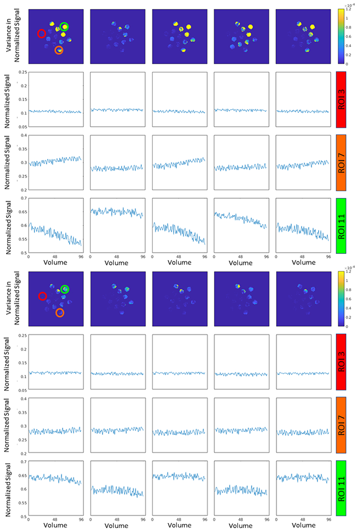
Empirical characterization of drift in the ice water phantom. This plot presents the variance in the ice water phantom in 10 different scans over the course of the session (1st and 4th row) and normalized signal intensity within three ROIs (indicated in the top left plot). The top four rows represent the first five scans in the series with the bottom four representing the last five scans. Note that areas of high variance in the top plot row correspond to ROI’s that have greater drift and require more substantial calibration. Of concern, observe that different ROI’s within same scan are drifting with opposite signs, hence spatial correction of the signal drift is required. Furthermore, over the course of the session, the pattern of drift changes with time and with region. This complex drift pattern is motivation for the proposed spatial-temporal drift correction model, TS.
Figure 2.
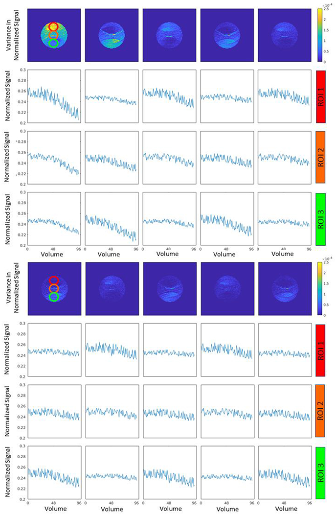
Empirical characterization of drift in the PVP phantom. This plot presents the variance in the PVP phantom in 10 different scans over the course of one session (1st and 4th row) and the normalized signal intensity within three ROI’s (indicated in the top left plot). The top four rows represent the first five scans in the series with the bottom four representing the last five scans. Observe the structural patterns in variance map that appear to correspond to parallel imaging artifacts. As with the ice water phantom (Figure 1), different ROI’s within same scan are drifting at different rates, and spatial correction is required. Similarly, the pattern of drift changes with time and with region.
To account for these effects, we proposed two key modifications. First, we generalize the ROI-temporal model to operate on a voxelwise basis to provide for a higher degree of spatial specificity in the correction while alleviating the need for external context information (i.e., the specification of ROI’s). Second, we propose a data-efficient model to capture the interaction effects between spatial and temporal nonlinearities. Herein, we combine these ideas to present a novel temporal-spatial model (TS) that accounts for the temporal instability of the scanner and spatial variation in the signal drift. We compare the new approach to uncorrected data, the temporal model (T) as proposed by Vos et al. [14], and a custom generalization of the Vos et al. that models nonlinearities on a voxelwise basis. The novel method yields greater improvement in error than the alternative approaches. This work highlights the need to capture interleaved b0 data in DWMRI and provides an effective model to capture patterns of signal drift within a scan while yielding more accurate estimation of directional ADC.
Data and Methods
Acquisition
Figure 3 outlines the process for acquisition and processing. Images are acquired on a Philips 3T MRI system. For both the ice-water phantom and the PVP phantom, 10 scans were acquired in a single session with 96 gradient directions at a b-value of 2000 s/mm2 and with a variable number of minimally weighted volumes of b=0.1 s/mm2 interspersed throughout the scans. The acquisition parameters for all scans are as follows: b-value of 2000 s/mm2, interspersed b-value of 0.1 s/mm2, TR of 8394 ms, TE of 70 ms, SENSE acceleration of 2.5, slice thickness of 2.5 mm, and in-plane pixel dimensions of 2.5 mm. The number of these minimally weighted volumes was decreased every two scans giving a pair of scans of opposite phase encoded directions (left phase encoding and right phase encoding) with 13, 7, 4, 3, and 2 minimally weighted volumes at the beginning, end, and interspersed among the 96 directions in that chronological order.
Figure 3.
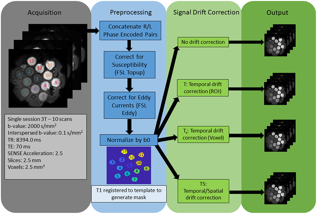
This shows our process from acquisition to correction. From the left, the acquisition parameters are shown, then the preprocessing pipeline, and finally the three different outputs resulting from the three different methods.
Preprocessing
Each pair of scans with opposite phase encodings and the same b-value was concatenated for preprocessing which consisted of topup for susceptibility distortion correction [15] and eddy current correction [16]. Within each scan, relative signal intensity images were computed by normalizing the diffusion weighted volumes by the first minimally weighted volume (“b0”) of the scan. Note that subsequent analyses were performed with additional b0-correction as described below. Next, each scan was registered to the T1 structural MRI of the phantom. The structural MRI’s were manually labeled using custom scripts in MATLAB (Mathworks, Natick, MA). For the ice-water phantom, the 13 ROIs correspond to the 13 vials of varying PVP concentrations. The spherical PVP phantom is simply filled with PVP at one concentration, and three spherical ROIs were defined within it to visually correspond to different regions as shown in Figure 2.
Signal drift correction
Each of the following correction methods was independently applied to each of the acquisitions, which resulted in five different output 4-D volumes for each scan: uncorrected images, images corrected using the Vos et al temporal model (T), images corrected using the Vos et al temporal model generalized to voxels (Tx), and images corrected using the temporal/spatial model (TS).
Method 1: Uncorrected.
No additional was processing was performed.
Method 2: Vos et al Temporal Model (T)
The model defined by Vos et al. estimates a global signal decrease with a linear or quadratic fit through the mean signal intensities of the interspersed b0 images within a region of interest. Figure 2 illustrates that the observed drift is non-linear, and so the linear model would not suffice. However, we apply a linear model when the number of b0 images is less than 3. The linear and quadratic models are defined for the ROI using the b0 volumes among the scanned images by:
| (1) |
and
| (2) |
respectively where n is the index of the volume; S (n) is the mean signal within the b0 image at time index n for the ROI; d, d1, and d2 are the modeled signal drift coefficients; and s0 is the signal offset at the b0 image where n = 0. After the linear fitting of s0, d1, and d2, a rescaling factor is used to correct each ROI:
| (3) |
and
| (4) |
where is the corrected signal intensity in the image normalized to 100 for quadratic corrections [14]. The linear model (Eq. 3) was applied when three or fewer b0’s were acquired, while quadratic model was applied when more b0’s were available.
Method 3: Vos et al. Generalized to Voxels (Tx)
The Vos model was modified to fit the signal time course to each voxel allowing free form spatial correction. In this case a single mask is provided which denotes voxels that are in any of the ROIs. The linear and quadratic models then become:
| (5) |
and
| (6) |
where V(X, n) is the signal intensity of the voxel at the xyz-coordinate in the image; X is the vector that specifies the xyz-coordinate; dX, d1,X, and d2,X are the modeled signal drift coefficients; and v0,X is the signal offset for the voxel in the b0 image where n =0. The rescaling becomes:
| (7) |
and
| (8) |
where V(X, n) is the uncorrected intensity for the voxel at the xyz-coordinate in image n, and corrected signal intensity for that voxel.
Method 4: Temporal/Spatial Model (TS)
We propose a new temporal/spatial (TS) model to take into account the temporal effects in the Vos model (e.g., Eq. 5–8), the spatial effects (e.g., as captured by the v0,X terms), and their interactions. The degrees of freedom in a model that allows for voxel-wise variations in the interaction between temporal and spatial effects would quickly become untenable. Rather, we propose to use a second order Chebyshev polynomial decomposition of the spatial effects, while interacting with a polynomial expansion of temporal effects (as in Eq. 5 and 6). In the linear TS model, the basis functions are:
| (9) |
| (10) |
| (11) |
and the combined linear TS model is:
| (12) |
For the quadratic model, the basis functions are:
| (13) |
| (14) |
| (15) |
| (16) |
and the combined quadratic TS model is:
| (17) |
where BT(X, n) has the same temporal components as T, and BTSv(X, n), BTSn(X, n), and BTSn2 (X, n) are the spatial-temporal components of the model that come from the cross product of three second order Chebyshev polynomials, each dealing with either the x, y, or z coordinate of the voxel. The rescaling in this method is defined by:
| (18) |
and
| (19) |
To better account for outliers, all coefficients were estimated using robust bi-square regression [17].
Analysis
For the analysis of the methods, values were calculated in terms of signal intensity and ADC. For the ice-water phantom, ROIs corresponding to three vials of different PVP concentrations and spatial locations were chosen and are denoted by the ROI numbers 3, 7, and 11 as shown in Figure 1. As for the spherical PVP phantom, the three ROIs selected correspond to the spherical ROIs as shown in Figure 2. For each diffusion volume in the 10 scans and for each method, the mean signal intensity and mean ADC was calculated for each ROI. The measurement of error within each ROI for every scan was calculated as the standard deviation of a third-degree polynomial fit to the mean ADC over the course of the scan. This metric quantifies the amount of residual drift across time. It also captures the variation from the isotropic properties of each ROI while ignoring the signal-to-noise ratio (SNR) variation between ROIs especially those of different PVP concentrations in the ice-water phantom. For the analysis of the number of b0 images needed, the same measurement of error is used, but only TS corrected images are used. The scans corrected using fewer than 13 interspersed b0 images for this analysis were artificially created by removing b0 images from both of the first two scans (those with 13 b0 images). To analyze the statistical difference between all methods, the ADC for all voxels in all scans in a valid ROI were considered for each method in a Wilcoxon rank sum test. In this way a p-value was generated for each pairing of methods.
Results
For both phantoms, the signal drift in ROIs of higher variance as seen in Figures 1 and 2 reached and sometimes surpassed 10% over the course of a scan without any correction. Correcting for the global signal drift as in T does result in improvement over the uncorrected method in most ROIs. However, without accounting for the different and rates of the drift, the method does not reduce the error in all ROIs. Tx and TS show similar performances with small differences.
The mean normalized signal intensity and the corresponding standard deviation across the entire session (all ten scans) is reported in Figure 4 and Figure 5 for the ice-water and PVP phantoms respectively. In both phantoms, Tx and TS have similar signal intensities. In the ice-water phantom the uncorrected method and T show a small difference. T performs more closely to Tx and TS for the PVP phantom.
Figure 4 .
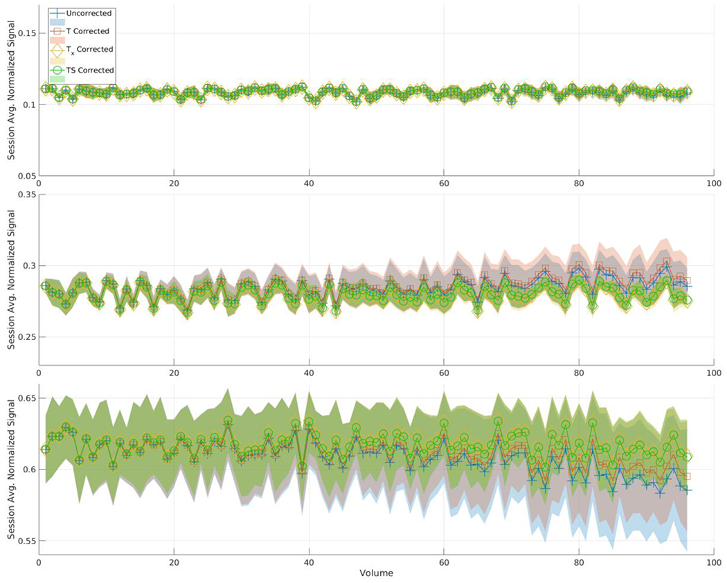
This plot represents the mean signal across the 10 scans in the session for the ice-water phantom for each method. Each line also has a shaded area representing the standard deviation among those scans at each volume number. Each plot represents one of the three selected ROIs from Figure 1. From top to bottom those ROIs are 3, 7, and 11. In ROI 3 there is no difference between the methods, but in the ROIs that show higher variance in Figure 1, the uncorrected method and T deviate from Tx and TS.
Figure 5.
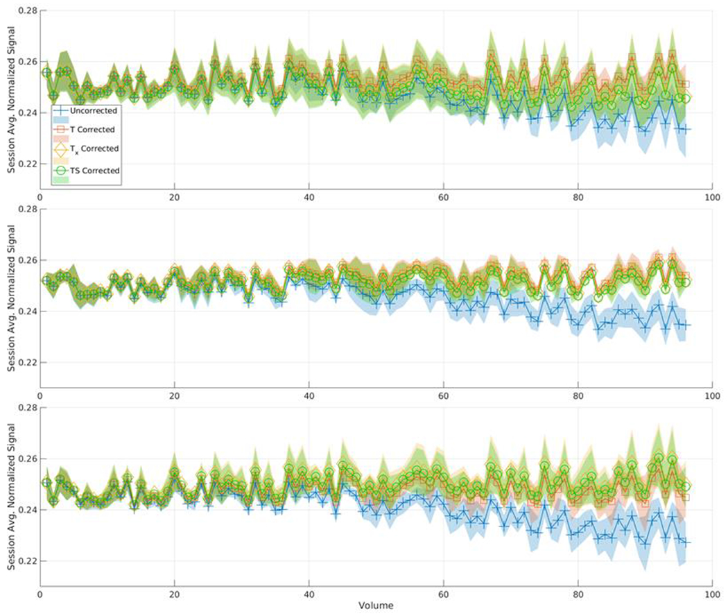
This plot represents the mean signal across the 10 scans in the session for the PVP phantom for each method. Each line also has a shaded area representing the standard deviation among those scans at each volume number. Each plot represents one of the three selected ROIs from Figure 1. From top to bottom those ROIs are 1, 2, and 3. In all 3 ROIs there is a noticeable difference between the uncorrected method and the correction methods. In ROI 1 and 3 there is also a slight difference between T and methods Tx and TS.
In Figure 6, the standard deviation of a third-degree polynomial fit to the mean ADC across diffusion volumes is reported for each method just as Figure 7 reports the same for the PVP phantom. The results for the ice-water phantom show the obvious shortcoming of correcting for the global signal drift. When a scan’s error is particularly large with no correction, Tx and TS outperform T, and in some cases when the ROI does not follow the global signal drift, T does worse than the uncorrected method whereas Tx and TS reduce the error. Figure 6 also shows the effects of leaving out b0 images from the first two scans (those with 13 interspersed b0s) and applying signal drift correction using TS. At the point where fewer than four b0 images are used, the linear model is used and is shown to be less stable in the two ROIs shown to have a higher variance in Figure 1.
Figure 6.
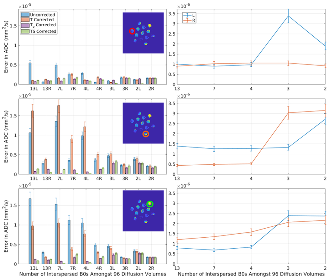
This plot presents the average error in ADC (standard deviation in a 3rd degree polynomial fit to the mean ADC of an ROI over the course of a scan) after correction for each of the five methods for 10 consecutive sessions using the ice water phantom with varying numbers of interspersed minimally weighted (“b0”) volumes (labeled in the x-axis). The appended letter of the x-axis label indicates the phase encoding direction (L = rll R= rlr). The three rows correspond to the three ROI’s in Figure 1, as indicated. The left column presents a comparison of the five methods. In the low variance ROI (first row), overall errors are small and little difference is observed between methods. In the two ROIs of higher variance, Tx, and TS outperform T for all scans. Note that in some scans, the uncorrected method out performs the T corrected scans. The right column studies simulated rate of b0 volumes by dropping out the b0s from the first two scans. Observe that with at least 4 b0s, the model errors are stable and low, which is intuitive as a second degree model is fit for #b0s>3 and a first degree model is fit for #b0<=3.
Figure 7.
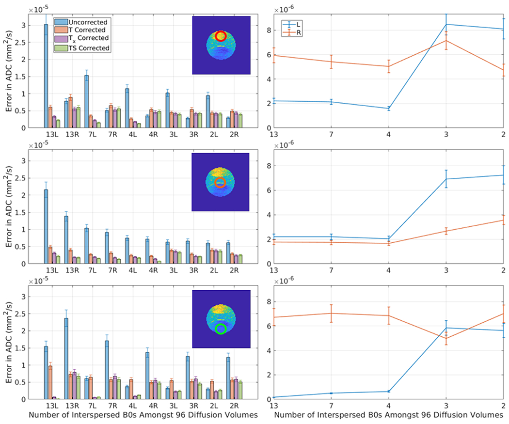
This plot presents the error in ADC (standard deviation in a 3rd degree polynomial fit to the mean ADC of an ROI over the course of a scan) after correction for each of the five methods for 10 consecutive sessions using the PVP phantom with varying numbers of interspersed minimally weighted (“b0”) volumes (labeled in the x-axis). The appended letter of the x-axis label indicates the phase shift direction (L = rll R= rlr). The three rows correspond to the three ROI’s in Figure 1, as indicated. The left column presents a comparison for the five methods. In the middle ROI (second row) T, Tx, and TS show very similar performance as the drift in the center ROI is similar to the average drift across all ROIs. In the outer two ROIs (especially row 3) Tx and TS shows significant improvements over T. The right column studies simulated rate of b0 volumes by dropping out the b0s from the first two scans. Observe that with at least 4 b0s, the model errors are stable and low, which is intuitive as a second degree model is fit for #b0s>3 and a first degree model is fit for #b0<=3.
Figure 7 shows similar results for the PVP phantom. The signal drift in the ROIs in this phantom agree with the direction of the global signal drift, but the rates at which the signal drift occurs within the ROIs varies. As a result, the errors in T and Tx and TS are not as significantly different—see for example ROI 7 (middle row) in Figure 6. The central ROI (ROI 2) agrees closely with the global signal drift, but the outer two ROIs show improvement when using Tx or TS as the spatial information becomes more necessary. In the right column in Figure 7, the effects of leaving out b0 images from the two scans that initially had 13 b0 images shows different results for the scan with right phase encoding. The scan with a left phase encoding direction shows an upward trend in error as fewer b0 images are used in all ROIs, but the scan with right phase encoding does not show a significant change (see Table 2 for all significance levels).
It can be seen from Figures 6 and 7 that even the scans with errors corresponding to a 10% difference in ADC due to drift can be corrected to error levels corresponding to a difference of less than 5%. Though methods Tx and TS perform very similarly in terms of error, it should be noted that the parameter space needed for fitting the Tx model is far greater than that of TS. Tx requires two parameters per voxel for the quadratic model while TS only requires a total of 81 parameters.
Discussion
Though Vos et al. most recently explored the signal drift caused by temporal instability of scanner systems in DWMRI, signal drift has been an issue in imaging systems that many have attempted to address. In functional magnetic resonance imaging, the effects of signal drift have been observed resulting in a few different methods for correction [18]. Gram-Schmidt orthogonalization [19] and high-pass filtering [20] have been used to eliminate signal drift, but other methods are very similar to Tx in that they model the temporal drift in a voxelwise manner using either a polynomial [21], a spline [22], or a wavelet [23]. Another method assumes that all voxels follow the trend of the global signal much like T and removes the global signal drift from each voxel [24]. However, we have seen that the assumption of a global trend does not always hold. As mentioned by Vos et al., most of these methods are fMRI specific as the drift is included as a confounding factor [14], but the premises can be adapted to DWMRI. Correction on an ROI basis is restricted by the defined ROIs, and therefore is not a commonly used method. TS is unique in that it models the spatial variation in the temporal drift where Tx allows the temporal models to be spatially independent and freely formed within a voxel.
It can be noted in Figure 6 that the error drops in the rlr phase encoded scan in the first ROI as two interspersed b0s are used instead of three, but the error is still higher than when using four or more b0s. Also, in Figure 7, the rlr phase encoded scans do not seem to have a particular trend as fewer b0s are used for correction. However, compared to the rll phase encoded scans denoted by 13L in the left column of Figure 7, the correction methods did not have as significant of an effect in the upper and lower ROIs for the rlr phase encoded scans denoted by 13R. We would expect if the resulting error is significantly reduced using all b0s available to the correction method then the error would have an upward trend as fewer b0s are used.
We find that we can correct even rather severe signal drift produced in an imaging situation intended to highlight the effects of the drift (e.g., isotropic phantoms with a large number of diffusion weighted volumes). Yet, to perform this correction a b0 is acquired at least every 32 volumes (or a minimum of 4 b0 volumes to support robust fitting of quadratic temporal models). For pragmatic technical reasons on the Philips systems, we use low (<5 s/mm2), but non-zero, diffusion sensitized volumes to enable repeated b0’s interleaved with volumes of higher diffusion weighting. Given the variable degree of signal drift observed within an imaging session and across similar phantoms, we strongly advocate for self-correction of individual datasets through interspersed b0’s. Fortunately, these data can be acquired without time penalty as standard practice is already to acquire b0’s in an approximate ratio of 8:1. All data have been made available via a SVN repository at: http://www.nitrc.org/scm/?group_id=1282.
Table 1.
For each method and for each phantom the median of the errors from all ROIs indicated in Figures 1 and 2 is reported here along with the inter quartile range (IQR) of the errors. Additionally symbols have been placed next to the median values to indicate the rejection of the hypothesis that the method is equivalent to Uncorrected (*), T (†), or Tx (‡). The hypotheses were evaluated at a significance level of 5% using the Wilcoxon rank sum statistical test. Here we see that TS has a lower median error, but Tx shows the lowest IQR.
| Method | Ice-water Med. Error | IQR | PVP Med. Error | IQR | ||||
|---|---|---|---|---|---|---|---|---|
| x 10−5 | x 10−5 | x 10−5 | x 10−5 | |||||
| Uncorrected | 0.35 | 0.35 | 0.85 | 0.76 | ||||
| T | 0.29 * | 0.37 | 0.51 * | 0.23 | ||||
| Tx | 0.16 * | 0.05 | 0.35 *† | 0.23 | ||||
| TS | 0.16 *†‡ | 0.10 | 0.28 *†‡ | 0.29 | ||||
Acknowledgements
This work was supported by R01EB017230 (Landman). This work was conducted in part using the resources of the Advanced Computing Center for Research and Education at Vanderbilt University, Nashville, TN. This project was supported in part by the National Center for Research Resources, Grant UL1 RR024975-01, and is now at the National Center for Advancing Translational Sciences, Grant 2 UL1 TR000445-06. The content is solely the responsibility of the authors and does not necessarily represent the official views of the NIH.
References
- 1.Catani M and De Schotten MT, A diffusion tensor imaging tractography atlas for virtual in vivo dissections, cortex, 2008. 44(8): p. 1105–1132. [DOI] [PubMed] [Google Scholar]
- 2.Jeurissen B, et al. , Investigating the prevalence of complex fiber configurations in white matter tissue with diffusion magnetic resonance imaging. Human brain mapping, 2013. 34(11): p. 2747–2766. [DOI] [PMC free article] [PubMed] [Google Scholar]
- 3.Reijmer YD, et al. , Improved sensitivity to cerebral white matter abnormalities in Alzheimer’s disease with spherical deconvolution based tractography. PloS one, 2012. 7(8): p. e44074. [DOI] [PMC free article] [PubMed] [Google Scholar]
- 4.Yogarajah M, et al. , Tractography of the parahippocampal gyrus and material specific memory impairment in unilateral temporal lobe epilepsy. Neuroimage, 2008. 40(4): p. 1755–1764. [DOI] [PMC free article] [PubMed] [Google Scholar]
- 5.Pierpaoli C, et al. , Water diffusion changes in Wallerian degeneration and their dependence on white matter architecture. Neuroimage, 2001. 13(6): p. 1174–1185. [DOI] [PubMed] [Google Scholar]
- 6.Jones DK, Knösche TR, and Turner R, White matter integrity, fiber count, and other fallacies: the do’s and don’ts of diffusion MRI. Neuroimage, 2013. 73: p. 239–254. [DOI] [PubMed] [Google Scholar]
- 7.Farrell JA, et al. , Effects of signal-to-noise ratio on the accuracy and reproducibility of diffusion tensor imaging–derived fractional anisotropy, mean diffusivity, and principal eigenvector measurements at 1.5 T. Journal of Magnetic Resonance Imaging, 2007. 26(3): p. 756–767. [DOI] [PMC free article] [PubMed] [Google Scholar]
- 8.Landman BA, et al. , Effects of diffusion weighting schemes on the reproducibility of DTI-derived fractional anisotropy, mean diffusivity, and principal eigenvector measurements at 1.5 T. Neuroimage, 2007. 36(4): p. 1123–1138. [DOI] [PMC free article] [PubMed] [Google Scholar]
- 9.Grech-Sollars M, et al. , Multi-centre reproducibility of diffusion MRI parameters for clinical sequences in the brain. NMR in Biomedicine, 2015. 28(4): p. 468–485. [DOI] [PMC free article] [PubMed] [Google Scholar]
- 10.Mirzaalian H, et al. , Inter-site and inter-scanner diffusion MRI data harmonization. NeuroImage, 2016. 135: p. 311–323. [DOI] [PMC free article] [PubMed] [Google Scholar]
- 11.Fortin J-P, et al. , Harmonization of multi-site diffusion tensor imaging data. Neuroimage, 2017. 161: p. 149–170. [DOI] [PMC free article] [PubMed] [Google Scholar]
- 12.Thesen S, Kruger G, and Muller E. Absolute correction of B0 fluctuations in echo-planar imaging, in Proceedings of the International Society of Magnetic Resonance in Medicine. 2003. [Google Scholar]
- 13.Benner T, et al. , Real-time RF pulse adjustment for B0 drift correction. Magnetic resonance in medicine, 2006. 56(1): p. 204–209. [DOI] [PubMed] [Google Scholar]
- 14.Vos SB, et al. , The importance of correcting for signal drift in diffusion MRI. Magnetic resonance in medicine, 2017. 77(1): p. 285–299. [DOI] [PubMed] [Google Scholar]
- 15.Andersson JL, Skare S, and Ashburner J, How to correct susceptibility distortions in spin-echo echo-planar images: application to diffusion tensor imaging. Neuroimage, 2003. 20(2): p. 870–888. [DOI] [PubMed] [Google Scholar]
- 16.Andersson JL and Sotiropoulos SN, An integrated approach to correction for off-resonance effects and subject movement in diffusion MR imaging. Neuroimage, 2016. 125: p. 1063–1078. [DOI] [PMC free article] [PubMed] [Google Scholar]
- 17.Dumouchel W and O’Brien F. Integrating a robust option into a multiple regression computing environment in Computing and graphics in statistics. 1992. Springer-Verlag New York, Inc. [Google Scholar]
- 18.Tanabe J, et al. , Comparison of detrending methods for optimal fMRI preprocessing. NeuroImage, 2002. 15(4): p. 902–907. [DOI] [PubMed] [Google Scholar]
- 19.Bandettini PA, et al. , Processing strategies for time-course data sets in functional MRI of the human brain. Magnetic resonance in medicine, 1993. 30(2): p. 161–173. [DOI] [PubMed] [Google Scholar]
- 20.Skudlarski P, Constable RT, and Gore JC, ROC analysis of statistical methods used in functional MRI: individual subjects. Neuroimage, 1999. 9(3): p. 311–329. [DOI] [PubMed] [Google Scholar]
- 21.Mattay VS, et al. , Whole-brain functional mapping with isotropic MR imaging. Radiology, 1996. 201(2): p. 399–404. [DOI] [PubMed] [Google Scholar]
- 22.Genovese CR, A Bayesian time-course model for functional magnetic resonance imaging data. Journal of the American Statistical Association, 2000. 95(451): p. 691–703. [Google Scholar]
- 23.Meyer FG, Wavelet-based estimation of a semiparametric generalized linear model of fMRI time-series. IEEE transactions on medical imaging, 2003. 22(3): p. 315–322. [DOI] [PubMed] [Google Scholar]
- 24.Macey PM, et al. , A method for removal of global effects from fMRI time series. Neuroimage, 2004. 22(1): p. 360–366. [DOI] [PubMed] [Google Scholar]


