Genomic Similarity and Kernel Methods II: Methods for Genomic Information

Abstract

Measures of genomic similarity are often the basis of flexible statistical analyses, and when based on kernel methods, they provide a powerful platform to take advantage of a broad and deep statistical theory, and a wide range of existing software; see the companion paper for a review of this material [1]. The kernel method converts information – perhaps complex or high-dimensional information – for a pair of subjects to a quantitative value representing either similarity or dissimilarity, with the requirement that it must create a positive semidefinite matrix when applied to all pairs of subjects. This approach provides enormous opportunities to enhance genetic analyses by including a wide range of publically-available data as structured kernel ‘prior' information. Kernel methods are appealing for their generality, yet this generality can make it challenging to formulate measures of similarity that directly address a specific scientific aim, or that are most powerful to detect a specific genetic mechanism. Although it is difficult to create a cook book of kernels for genetic studies, useful guidelines can be gleaned from a variety of novel published approaches. We review some novel developments of kernels for specific analyses and speculate on how to build kernels for complex genomic attributes based on publically available data. The creativity of analysts, with rigorous evaluations by applications to real and simulated data, will ultimately provide a much stronger array of kernel ‘tools' for genetic analyses.

Introduction

Evaluating the relationship of genetic information with phenotypes is becoming increasingly complex because of the large amount and diversity of genetic data. Traditional regression models, whether for quantitative or categorical traits, are challenged by the high-dimensionality of genomic data, where the number of genomic ‘predictor' variables is much larger than the number of independent subjects. Alternative approaches are needed for high-dimensional data to improve testing of focused hypotheses that might be based on prior information (e.g. genetic pathways), to improve prediction of traits based on genetic data, and to improve model selection. Furthermore, integrating disparate types of genetic information, such as gene expression, genetic variants (e.g. single-nucleotide polymorphisms, SNPs), copy number variants, or even the DNA sequence itself, is quite challenging, yet potentially highly informative. A flexible approach that provides a framework to achieve these objectives can be based on kernel methods that use measures of similarity between pairs of subjects, as discussed in the companion paper [1].

This companion paper reviewed the desirable mathematical properties of similarity measures that create positive semidefinite (psd) kernel matrices, and the corresponding statistical models and software that can be applied to kernel matrices. Furthermore, the mathematical basis of how to construct ‘valid' psd kernels was reviewed.

The focus of this paper is on ways to create kernels for measures of genetic similarity. As a start, a few concrete examples of similarity measures used in genetic studies have been the fraction of alleles alike-in-state across a large number of genetic markers, or quantitative scoring of haplotype sharing for pairs of subjects. Other examples are discussed in the companion paper [1]. The goal of our review of a variety of novel kernels that have been developed over the years for a wide variety of scientific aims is to illustrate by examples the potential merits of different kernels, and to provide intuition on how to build new kernels for new types of data or new scientific aims. We begin with a variety of similarity kernels, and then switch to measures of dissimilarity, which at times can be more direct than creating a measure of similarity. Finally, we speculate on how genomic information can be used to construct kernels, such as genomic pathway and network information, and how kernels can adapt to information as our understanding of complex genetic mechanisms evolves.

Similarity Kernels

General Coefficient of Similarity

Kernels that might prove useful for genomic data can be based on a general coefficient of similarity proposed by Gower [2]. His procedure first measures similarity on a given attribute, and then sums similarity scores over all attributes. Advantages of his general coefficient are that it allows for different types of attributes (dichotomous, categorical, and quantitative), it allows use of weights when summing over attributes, and it is psd if there are no missing data. The similarity score for subjects i and j for attribute k is denoted s_ijk. To account for a noninformative comparison, such as when data for an attribute are missing, an indicator variable is used: δ_ijk = 1 for an informative comparison, and 0 otherwise. Gower's general measure of similarity is

an average similarity over all p attributes, with the denominator count adjusted for the number of informative comparisons among all p attributes. The values of the s_ijkscores depend on whether the attribute is dichotomous, categorical, or quantitative.

For a dichotomous attribute with levels C and R, where C means common level and R means rare level, matching on R is counted, but not matching on C – matching on the common C level is not very informative for a similarity measure. In fact, the C/C pairs are excluded altogether by setting the indicator variable δ_ijk = 0 for a C/C pair, and 1 otherwise. An alternative interpretation for excluding the C/C pairs is when C means truly absent, such as a negative antibody test. If all attributes are dichotomous and none are missing, S_ij = a/(a + b + c), where the counts a, b, and c are for the pairs R/R, R/C, and C/R, respectively (the C/C pairs have a count of d, so that the total number of attributes is a + b + c + d = p). Alternative ways to account for the C/C pairs, and to weight the other types of pairs, are given in table 3.3 of [3].

For a categorical attribute, Gower used the ‘matching' kernel, with value 1 for matching categorical levels and 0 for a mismatch. For the special case of all attributes having only two levels and no missing data, this score results in S_ij = (a + d)/(a + b + c + d), illustrating that this measure includes matching on common levels, unlike the preceding measure that excludes them.

For a quantitative attribute, Gower used S_ijk = 1 – | x_ik – x_jk |/R_k, where R_k = max_ij{| x_ik – x_jk |}, or the range of attribute k. Gower showed that each of the proposed similarities (dichotomous, categorical, quantitative) is psd, so the sum over all attributes is psd. He further generalized the similarity to allow weights to differ across attributes,

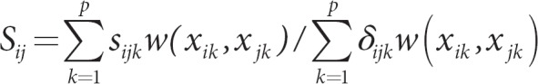
where the weight w(x_ik, w_jk) can depend not only on the attribute k, but also on the observed attributes for subject i and j, for example giving greater weight for matches on rare levels than on common levels. If there are no missing data, and w(x_ik, w_jk) ≥ 0, then the weighted total similarity is psd.

Gower's similarity measure offers significant advantages for genomic data: (1) it allows different ways to score marker genotypes (e.g. SNP genotypes scored as categorical variables with three levels, or as quantitative attributes having the values 0, 1, or 2 according to the number of copies of the rarer allele, as used by Zhang and Zhao [4]); (2) quantitative measures, such as gene expression assays, can be combined with SNP genotypes; (3) weights can be used, such as weights that depend on extraneous information. This would be a way to emphasize SNPs that are known to be in a chromosomal region of linkage reported in prior studies, or believed to be functional, or are in a biological pathway of interest.

Polynomial Kernels

Some examples of building kernels from other kernels are worth reviewing for their insights. A kernel created by a polynomial of a dot product is frequently used in machine learning. For example, Decoste and Schölkopf [5] found a 9th-degree polynomial to give good predictions of actual numbers from hand-written numbers for a kernel in support vector machines (SVMs). Some insight about a polynomial of a dot product can be gained by examining the 2nd-degree polynomial:

The expanded sum illustrates that all possible 2nd-degree products of each of x and y are used. The ordered product x_ix_j is called a ‘monomial' of degree 2, and so the above expansion can be written as a dot product of monomials of x with monomials of y, <$$>, where $$ represents the vector of all possible ordered products of degree 2. This illustrates that a 2nd-degree polynomial measures the similarity of pairs of attributes (e.g. x_ix_j) between subjects, capturing pair-wise correlation of attributes.

The intuition of polynomials capturing higher-order correlations of attributes was cleverly used by Zien et al. [6] to build a ‘pyramid' kernel to predict protein translation initiation sites from DNA sequences. They wanted to create a kernel that could scan a DNA sequence for translation initiation sites, allowing for local correlations of DNA sequences while down-weighting long range correlations. This idea would be analogous to allowing for local correlations of SNPs due to linkage disequilibrium (LD) while scanning for patterns that predict case/control status, and down-weighting long-range LD. To build a kernel to scan two nucleotide sequences, x and y, they first created a core kernel for perfect matching at nucleotide position t: k_t(x, y) = 1 if x_t = y_t, 0 otherwise. Next, they created a kernel for a window around position t, with the objective to allow local correlations within windows, and use weights (w_j) that increase from the boundaries of the window to the center of the window,

The polynomial of degree p₁ allows for local correlations within the window (window size of 2l + 1) that is centered on position t. The degree p₁ determines the number of nucleotides involved in the correlations (e.g. p₁ = 2 for all possible pairs of nucleotides; p₁ = 3 for all possible triples, etc.). The final step to create the ultimate kernel was

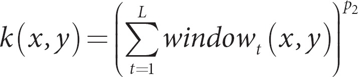
The sum is over all L nucleotide positions, and the polynomial degree p₂ was used to account for long-range correlations. When using this kernel with SVMs, they found that small windows that allowed for local correlations, yet no long-range correlations (p₂ = 1), performed well. This example nicely illustrates the expressive power to build kernels with other kernels, and to develop kernels specific to the type of data and aims of the study.

Kernels for Strings and Sequence Data

Kernels have also been used to compare character strings, such as DNA or protein sequences. A useful kernel that measures the similarity for two strings, s and t, is based on a weighted sum, where the sum is over all common substrings from s and t, and weights according to substring frequency and lengths. Some extensions have allowed for a few mismatches between strings, which might occur from measurement error, or mutation (see [7], p. 1,182 and [8]). Although string kernels and our prior discussion on polynomial kernels mainly have been used to analyze properties of the sequence itself, they should prove useful to evaluate the association of combinations of genetic variants (e.g. SNPs), or DNA sequences, with traits.

Prior Probability Kernels

At times it might be worthwhile to use probability models to build prior information into kernels. One approach, called Fisher kernels [7, 8, 9], is based on the probability density of attributes, p(x | θ), where θ is a vector of parameters. In a sense, the probability density measures how close x fits the model, with better fits giving higher probabilities. This can then be translated to a measure of similarity such that two subjects will have a higher similarity score if they both have high probabilities for their attributes. This is achieved by creating the score vector for θ, U(x) = ∂ln p(x | θ)/∂ θ, and using it in a dot product,

For exponential distributions, this kernel gives a reproducing kernel Hilbert space (RKHS; see [1]) whose inner product is based on sufficient statistics, an appealing strategy to begin building kernels. An alternative is to normalize the kernel by Fisher's information, I = E_x[U(x)U'(x)], to create the kernel K(x_i, x_j) = U' (x_i)I⁻¹ U(x_j). Although it may be difficult to specify a joint probability density for all attributes, it might be possible to specify a composite pseudo-density that captures some of the main features (e.g. marginal and pair-wise probabilities), similar to how composite likelihoods are used to obtain unbiased parameter estimates [10]. More work along these lines might prove useful for creating efficient robust kernels for genomic data.

An alternative probabilistic approach, called marginalized kernels [11], uses the expectation of a kernel, with the expectation taken over unobserved latent variables. If y_i is an unobserved latent variable that can have values in a finite set H (e.g. H having values of 1 or 0 for presence or absence of disease), and x_i is a vector of attributes, then the marginalized kernel is

where p(y_i | x_i) is the probability of latent variable y_i conditional on x_i and a set of parameters that links the two, and K₁([y_i, x_i], [y_j, x_j]) is a kernel for the combined variables [y_i, x_i]. To make this concrete, suppose y_i has values 1 or 0 for presence or absence of disease, x_i is a SNP genotype, and p (y_i | x_i) is the logistic regression model with assumed values for the regression coefficients, perhaps based on prior published reports for the anticipated effect size of SNPs on the risk for disease. Further, assume that K1 has the form

where K₂(y_i, y_j) is a match kernel, with value of 1 for a match and 0 otherwise, and K₃(x_i, x_j | y_i, y_j) is a kernel for the SNPs, noting that K₃ can change for different pairs of y values. The resulting marginalized kernel is

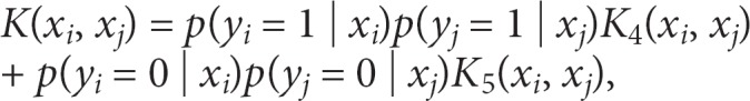
a weighted average of kernels for pairs of diseased subjects (K₄) and for pairs of non-diseased subjects (K₅). This approach uses prior information about the expected effect size of SNPs, or even combinations of SNPs, to build kernels. Because the prior information is built directly into the analysis, potentially strengthening the signals, it might prove more useful than using prior information to weight p values in genome-wide association studies [12, 13, 14], and avoids the complication of p values influenced by both the effect size and information content (e.g. allele frequencies) of SNPs.

Splines and Kernels

Spline functions are often applied to quantitative covariates to build nonparametric regression models, such that the influence of covariates can be flexibly modeled without prior assumptions (e.g. linear or quadratic effects of covariates on the trait mean). These approaches might prove useful for quantitative genetic information, such as gene expression data, or even quantitative scores of multiple SNPs (e.g. the sum of minor alleles of SNPs in a priori specified genetic pathways). Furthermore, nonparametric modeling provides a flexible framework to explore interactions of genes, or groups of genes. Fortunately, spline functions are closely tied to kernel methods. For example, if the columns of a design matrix are the bases of spline functions, such as piece-wise polynomials, then the resulting kernel based on the inner product can be used for spline smoothing in nonparametric regression [15]. More general spline smoothing, and its relationship to kernels, is clearly developed by Wahba [16]. For example, Wahba has published extensively on smoothing-spline ANOVA, which is a general nonparametric approach to flexibly model the main effects of attributes with nonparametric functions (to be estimated by kernels) and nonparametric interaction functions,

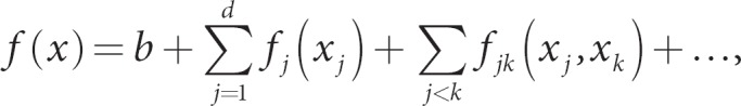
where b is a constant, f_j(x_j) is a nonparametric function for the main effect of attribute j, f_jk(x_j, x_k) is a nonparametric function for two-way interaction, and ‘…' indicates that higher-order interactions could be modeled nonparametrically. When attributes are coded as numeric vectors, say vectors x and y, and scaled to range over [0, 1], the kernel that corresponds to this smoothing spline ANOVA is

Although smoothing spline ANOVA has not yet been used for modeling genetic data, its utility for guiding interpretations of epidemiological studies has been demonstrated [17, 18]. suggesting that this flexible framework might prove useful for high-dimensional genetic information, particularly when a goal is to evaluate the role of interactions. Discussions of other types of kernels for a range of complex data types, such as hierarchically structured trees, or graphs (vertices connected by edges), can be found in [7, 8, 9].

Dissimilarity Kernels

Although most kernel methods focus on measures of similarity, at times it can be easier to first create a measure of distance, and then transform it to similarity, such as the gaussian kernel that transforms the euclidean distance between two vectors, or Gower's method that transforms absolute distance. Gower and Legendre [19] evaluate commonly used dissimilarity measures for binary and quantitative attributes according to whether they correspond to euclidean distances, a good resource when devising new dissimilarity measures for genomic data. In some contexts, it might be more direct to devise a measure of dissimilarity that is not necessarily euclidean distance. However, be cautious. Dissimilarities are often not psd, and simple conversions to a measure of similarity may not result in a psd matrix. There is a way around this. Any dissimilarity matrix with elements d_ij can be transformed into a matrix with elements e_ij that have euclidean distances (e_ij = $$ or e_ij = d_ij + c₂, where c₁ and c₂ are determined from the eigenvalues of transformations of the dissimilarity matrix (see p. 43 of [3]; [19], and corrections in [20]). This allows one to develop a general dissimilarity measure that can be transformed to euclidean distances, and then transformed by a gaussian kernel to a psd similarity measure.

An alternative approach to using dissimilarity measures in machine learning is to use conditionally positive definite kernels. Recall that K is positive definite if c'Kc > 0 for all c ≠ 0. Although this might not be true for all c ≠ 0, there might be a subset of c's for which this is true. A constraint on c that can sometimes works is Σc_i = 0. To see this, consider the kernel for squared euclidean distance, and evaluate whether it is psd:

At this point, we cannot conclude whether the kernel is psd, but if we restrict Σc_i = 0, the first two terms drop out illustrating that

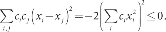
So, the squared euclidean distance is not psd, but its negative value is conditionally psd. Conditionally psd kernels have been used in SVM algorithms, because they have an implicit mapping to an associated psd kernel in the underlying RKHS [9]. This approach might pay off for other types of penalized regression models.

Speculations on Kernels for Genomic Information

Up to now, we have reviewed a number of novel strategies to construct kernels, yet with little attention to biological information. Determining whether genetic variation has direct causes on the variation of phenotypes is the challenging holy grail for human genetics in general, and genomic medicine in particular. The true benefit from using kernels will be realized only when kernels are developed and tested for specific scientific studies. Fortunately, the diversity and amount of genomic information that can be used to create kernels is growing at an astounding rate. Although the many aspects relevant for predicting function from genetic information are far beyond the scope of this review, we provide some speculative ideas in the next few sections about how kernels could be created from genomic information, ranging from information on functional scores to biologic pathways to systems biology networks.

To simplify our exposition, we restrict ideas about function to SNPs, recognizing that other genomic information, such as copy number variants or gene expression, could easily be used to create kernels. SNPs can be classified into different categories of likely function, such as those that might influence protein sequence variation. For example, exonic coding SNPs that are nonsynonymous (missense mutation) cause changes in a codon that result in a change in amino acid. These types of variants can affect enzyme kinetics, DNA-binding proteins that regulate transcription, signal transduction of transmembrane proteins, or structural proteins. Synonymous SNPs in exons do not change amino acid, but this does not necessarily mean that function is not altered. Other types of SNP variations can occur in introns, cause nonsense mutations (causing a premature stop codon, resulting in a truncated protein sequence) or frameshift mutations. Variants can also occur in splicing sequences, motifs, or exonic splicing enhancers. SNPs can also influence the regulation of gene expression, such as promoter or repressor variants. Any of these types of variation could influence the function of genes, but probability of functional impact can vary widely. For reviews on some of these ideas, see [21, 22]. With this range of classification, kernels can be created to quantify similarity of SNPs according to their likely function. Suppose that a similarity matrix S is created to score similarity of functions for P SNPs. To map from SNP-similarity to subject-similarity, one could use XSX', where X is an N × P design matrix of indicator variables for presence/absence of functional genotypes, or for counts of functional alleles within genotypes.

Some typical ways to evaluate the likelihood of function of genetic variants are comparative genomics and computational functional genomics. Comparative genomics compares DNA, RNA, or protein sequences between different species to search for signatures of natural selection (positive/negative and strength of selection pressure), regions of high conservation, regulatory regions, or even ultra-conserved regions with long stretches of DNA that do not appear to code for proteins. Computational functional genomics uses gene transcription, translation, and protein-protein interactions to create scores for likely function. For example, the popular SIFT algorithm (‘sorting intolerant from tolerant') evaluates protein sequences for amino acid substitutions using position-specific information derived from sequence alignments, and requires only sequence and homologue information, resulting in a tolerance index. In contrast, Poly-Phen uses a wide variety of features that are sequence-, evolutionary- and structurally-based to predict whether a nonsynonymous mutation is likely to affect protein function, and performs optimally if structural information is available. Generally, the quality of a method will depend on the amount of input data available (see [21] for more thorough comparisons of software and their URLs). These scores of likely function are often based on measures of similarity of a ‘test' sequence with a sequence of known function, providing a basis for building kernels for pairs of sequences.

Finally, there are many publically available databases that provide information on gene function, disease polymorphisms, etc. For example the Nucleic Acids Research online Molecular Biology Database Collection is a public repository that lists more than 1,000 databases (http://www.oxfordjournals.org/nar/database/c/). Some of the major database categories are: nucleotide sequences, RNA sequences, protein sequences, genomics (human, other vertebrae, and nonvertebrae), metabolic and signaling pathways, human genes and diseases, microarray and other gene expression, proteomics, drugs and drug design, mitochondrial genes and proteins, and immunological data. Alternatively, Pathguide contains information for about 240 biological pathway resources (http://www.pathguide.org/), with major categories of protein-protein interactions, metabolic pathways, signaling pathways, pathway diagrams, transcription factors/gene regulatory networks, protein-compound interactions, genetic interaction networks, and others.

The preceding examples illustrate the rich and growing resources to predict function of genomic information, often through ‘guilt by association'. That is, scoring SNPs or other types of genomic variation for their likely function is based on the inherent logic of similar genomic features implying similar function. Kernels are the natural language of similarity metrics, providing the link from complex measures of genetic similarities to their associations with traits.

Kernels for Genomic Pathways

Pathway analyses, popular yet nondescript, are ways to include prior knowledge, often applied to gene expression analyses. Most take advantage of gene annotation from Gene Ontology [23] and KEGG Pathway [24]. Two popular ‘pathway' analyses have focused on the distribution of p values (for the association of genetic variants with phenotypes), to determine if small p values tend to cluster in particular components of a pathway. The first approach is to search for an overrepresentation of significant associations (using an arbitrary p value cutoff) in a particular pathway relative to the rest of the tested associations, to determine if differentially expressed genes are overrepresented in a particular pathway. The second approach, called gene set enrichment analysis, compares the entire distribution of test statistics in a pathway to the rest of the genes [25, 26], and has been extended to association studies with SNPs [27]. Although simple to implement and interpret, pathway analyses based on simple p values do not take full advantage of complex data sets. Recent developments, based on random effects models, provide more rigorous and efficient analyses. For example, Wang et al. [28] developed a linear mixed model to evaluate the covariation in gene expression among genes that occur within the same pathway. Although this novel approach used a simple random effects model to estimate three variance components (arrays, pathways, and residual error), it represents a step toward using more elaborate kernels to structure the prior information, as we emphasized in the companion paper on the link between a structured covariance matrix for random effects and a kernel matrix [1]. For example, a kernel matrix that encodes similarity among SNPs according to whether they occur in common pathways could allow for ambiguity, such as using weights ranging 0–1. Furthermore, the kernel matrix would automatically account for partially overlapping pathways. Hence, the kernel method provides ample opportunities to create more refined analyses.

From Networks to Kernel Matrices

It is important to recognize that networks can be mapped into a kernel matrix. Networks are typically represented by graphical structures, with nodes (i.e. vertices) connected by edges. The edges can represent the strength of linkage between nodes, so that no linkage means an edge has a value of 0, and stronger linkage means a larger edge value. Edges can be standardized to range from 0 to 1, so that edges represent strength of similarity between nodes. If a graph has N nodes, it can be mapped to an N × N matrix K, with K_ij representing the edge weight between nodes i and j. We can then interpret K to represent the similarity between all pairs of nodes, a kernel matrix.

Organizing genomic information into networks is common in systems biology research and is a convenient way to represent and analyze interactions among genes, among proteins, and coexpression of mRNA levels. Furthermore, networks can be built upon other networks. To illustrate this by a hypothetical example, suppose we wish to create a similarity matrix for SNPs, based on how the SNPs are related to each other through gene expression. First, consider an experiment with n different genes measured for their mRNA expression. These expression values can be standardized to have a normal distribution and their marginal covariance matrix, V (dimension n × n), can be estimated. A graphical model for gene expression can then be created by using V to estimate a matrix of partial correlations, R. Partial correlations with a value of zero mean that edges in a graph can be removed. Although it can be challenging to estimate partial correlations when the number of measured genes is much larger than the number of independent samples, recent developments provide reasonably efficient and robust results [29, 30]. Furthermore, suppose that each expression probe is regressed on SNPs, using a regularized regression, such as lasso, to select SNPs. This would allow the SNPs to be overlaid on the network of gene expression levels. We could then create pathways between SNPs by following the links from a SNP to expression levels of another SNP. Following all possible pathways between pairs of SNPs would provide a way to create a measure of similarity between the pairs, a kernel matrix. For example, the weight for a given pathway can be estimated by using ideas from path analysis, multiplying path coefficients (standardized multiple regression coefficients) along the edges of a path [31]. The total weight for a pair of SNPs would then be the sum of the path weights, summed over all paths connecting the pair of SNPs. Although the development of this type of statistical framework needs more rigor, and limitations due to high-dimensional data evaluated, this hypothetical example illustrates the enormous flexibility provided by the kernel method.

Kernels to Model Evolving Knowledge of Genomics

Flexible methods are needed to model genomic knowledge for association studies, both hard and soft knowledge. Our understanding of gene function, for instance, is rapidly evolving. A flexible framework to model genomic information can be based on graphical models and networks, as emphasized in systems biology research. Fortunately, kernel methods can be built on network models, as discussed above. But, it is worthwhile to first consider the rationale for using networks to represent genomic information in general, and gene function in particular.

The views of Fraser and Marcotte [32] provide a sound basis to consider the advantages of using networks to analyze and describe gene function. They discuss two rational hierarchical strategies: ‘top-down' and ‘bottom-up'. The top-down approach is illustrated by the Gene Ontology project. It involves defining an almost comprehensive list of gene function categories, organizing them into a hierarchy, and then fitting individual genes into the categories. Gene Ontology uses three main categories: molecular function, biological process, and cellular component. The choice of categories, their hierarchical organization, and the assignment of genes into the categories are all completed through meticulous manual curation – not only labor-intensive, but often subjective.

In contrast, the bottom-up approach uses statistical methods to integrate multiple data sets, generating networks of gene linkages. Attributes of networks can be extracted and used as the framework for describing and categorizing gene function. In the bottom-up view, a gene's ‘profession' is interacting with other genes. A key difference between these two approaches is that the top-down fixes the functional hierarchy by the subjective manual curation of the underlying data, in contrast to the bottom-up that allows the data to reveal the hierarchy. The bottom-up approach also provides a flexible framework to iteratively improve the linkages as knowledge is gained.

For the bottom-up approach, Fraser and Marcotte [32] take a probabilistic view of gene function. This allows one to deal with diverse data sets (e.g. protein interaction data, microarray coexpression data, genetic variation data) and to separate signal from noise. Statistical methods are needed to account for noisy data sets, ultimately providing statistical measures of data quality, so that weights that correspond to data quality can be used to link genomic features. That is, interactions from each data set can be weighted according to their measured performances on benchmarks, and interactions can be assigned a joint confidence based on the combined weight of evidence. This measurement of error and weighted association between genes is the essence of the bottom-up approach, hence implicitly based on kernel functions. There are many different schemes for establishing the weights of each data set based on its underlying errors, such as bayesian statistics used for scoring interactions, or heuristic or other probabilistic approaches.

Note that the bottom-up approach leads to a probabilistic description of gene function. Not only are the links between genes weighted, but so too is the description of a biological process and the relative involvement of a gene in that process. These probabilistic connections arise in part from experimental uncertainty and in part from the stochastic nature of protein function. Fraser and Marcotte use this framework to define the function of a gene according to where it resides in the network and the probabilistic paths that link it to attributes. The organization of the attributes, their interconnections and the locations of each gene in this network are determined from the data and form a hierarchical framework, or perhaps a network, for describing gene function.

From a biologist's viewpoint, it might seem unnatural to consider the function of a gene as probabilistic. Yet, like the physicist requiring statistical principals from quantum mechanics to describe how subatomic particles interact, geneticists are beginning to recognize the need to include more statistical modeling in the definition of a gene and how its submolecular components interact to better describe gene sequence and function. This is familiar to statistical geneticists who have long used statistical models to link observed phenotypes with underlying unobserved genotypes. Now, the phenotype is more sophisticated, such as mRNA expression levels, or the DNA sequence itself. For example, in light of the complexity of the genetic architecture revealed by the ENCODE project, Gerstein et al. [33] state: ‘In the context of interpreting high-throughput experiments such as tiling arrays, the concept of a gene has an added practical importance – as a statistical model to help interpret and provide concise summarization to potentially noisy experimental data.' They further propose a tentative definition of a gene: ‘A gene is a union of genomic sequences encoding a coherent set of potentially overlapping functional products'. This somewhat abstract definition allows for a gene product to be a regulatory RNA, or a protein sequence, while allowing for different genomic subsequences, all from a given ‘gene', that code for different protein sequences due to alternatively spliced transcripts, for example. From this viewpoint, transitioning from probabilistic interactions within networks to kernel methods is a natural step towards using kernel methods.

Summary

The opportunities to enhance genetic analyses by including a wide range of publically-available data as structured kernel ‘prior' information are enormous, and the kernel methods outlined in this review provide the necessary statistical and computational framework. The challenge will be creating powerful kernel methods that filter the signal from the noise. Interesting questions remain, such as whether kernels for disparate data types should be summed to create a ‘total' kernel, or analyzed separately in a joint analysis [34]. This review provides some guidelines, and speculations, on how to build kernels for complex genomic attributes. Ultimately, the creativity of analysts, with rigorous evaluations by applications to real and simulated data, will provide a stronger array of kernel ‘tools' for genetic analyses.

References

- 1.Schaid D. Genomic similarity and kernel methods I: Advancements by building on mathematical and statistical foundations. Hum Hered. 2010;70:109–131. doi: 10.1159/000312641. [DOI] [PMC free article] [PubMed] [Google Scholar]
- 2.Gower J. A general coefficient of similarity and some of its properties. Biometrics. 1971;27:857–874. [Google Scholar]
- 3.Everitt B, Landau S, Leese M. Cluster Analysis, ed 4. London, Arnold. 2001 [Google Scholar]
- 4.Zhang S, Zhao H. Quantitative similarity-based association tests using population samples. Am J Hum Genet. 2001;69:601–614. doi: 10.1086/323037. [DOI] [PMC free article] [PubMed] [Google Scholar]
- 5.Decoste D, Schölkopf B. Training invariant support vector machines. Mach Learn. 2002;46:161–190. [Google Scholar]
- 6.Zien A, Rätsch G, Mika S, Schölkopf B, Lengauer T, Müller KR. Engineering support vector machine kernels that recognize translation initiation sites. Bioinformatics (Oxford, England) 2000;16:799–807. doi: 10.1093/bioinformatics/16.9.799. [DOI] [PubMed] [Google Scholar]
- 7.Hofmann T, Schölkopf B, Smola A. Kernel methods in machine learning. Ann Stat. 2008;36:1171–1220. [Google Scholar]
- 8.Christianini N, Shawe-Taylor J. An Introduction to Support Vector Machines and Other Kernel-Based Learning Methods. Cambridge, UK, Cambridge University Press. 2000 [Google Scholar]
- 9.Schölkopf B, Smola A. Learning with Kernels: Support Vector Machines, Regularization, Optimization, and Beyond. Cambridge, MA, MIT Press. 2002 [Google Scholar]
- 10.Lindsay BG. Composite likelihood methods. Contemporary Mathematics. 1988;80:221–239. [Google Scholar]
- 11.Tsuda K, Kin T, Asai K. Marginalized kernels for biological sequences. Bioinformatics (Oxford, England) 2002;18((suppl 1)):S268–S275. doi: 10.1093/bioinformatics/18.suppl_1.s268. [DOI] [PubMed] [Google Scholar]
- 12.Ionita-Laza I, McQueen MB, Laird NM, Lange C. Genomewide weighted hypothesis testing in family-based association studies, with an application to a 100k scan. American journal of human genetics. 2007;81:607–614. doi: 10.1086/519748. [DOI] [PMC free article] [PubMed] [Google Scholar]
- 13.Roeder K, Bacanu SA, Wasserman L, Devlin B. Using linkage genome scans to improve power of association in genome scans. Am J Hum Genet. 2006;78:243–252. doi: 10.1086/500026. [DOI] [PMC free article] [PubMed] [Google Scholar]
- 14.Roeder K, Devlin B, Wasserman L. Improving power in genome-wide association studies: weights tip the scale. Genet Epidemiol. 2007;31:741–747. doi: 10.1002/gepi.20237. [DOI] [PubMed] [Google Scholar]
- 15.Ruppert D, Wand M, Carroll R. Semiparametric Regression. New York, Cambridge University Press. 2003 [Google Scholar]
- 16.Wahba G, Smoothing splines in nonparametric regression . Encyclopedia of Environmetrics. In: El-Shaarawi A, Piegorsch W, editors. New York, Wiley. vol 4. 2001. pp. pp 2099–2112. [Google Scholar]
- 17.Lin X, Wahba G, Xiang D, Gao F, Klein R, Klein B. Smoothing spline ANOVA models for large data sets with Bernoulli observatrions and the randomized GACV. Ann Stat. 2000;28:1570–1600. [Google Scholar]
- 18.Wahba G, Wang Y, Gu CK, Klein B. Smoothing spline anova for exponential families, with application to the Wisconsin epidemiological study of diabetic retinopathy. Ann Stat. 1995;23:1865–1895. [Google Scholar]
- 19.Gower J. Metric and euclidean properties of dissimilarity coefficients. J Classification. 1986;3:5–48. [Google Scholar]
- 20.Legendre P, Anderson M. Distance-based redundancy analysis: Testing multispecies responses in multifactorial ecological experiments. Ecol Mongr. 1999;69:1–24. [Google Scholar]
- 21.Mooney S. Bioinformatics approaches and resources for single nucleotide polymorphism functional analysis. Brief Bioinform. 2005;6:44–56. doi: 10.1093/bib/6.1.44. [DOI] [PubMed] [Google Scholar]
- 22.Rebbeck TR, Spitz M, Wu X. Assessing the function of genetic variants in candidate gene association studies. Nat Rev. 2004;5:589–597. doi: 10.1038/nrg1403. [DOI] [PubMed] [Google Scholar]
- 23.Ashburner M, Ball C, Blake J, Botstein D, Butler H, Cherry J, Davis A, Dolinski K, Dwight S, Eppig J, Harris M, Hill D, Issel-Tarver L, Kasarskis A, Lewis S, Matese J, Richardson J, Ringwald M, Rubin G, Sherlock G. Gene ontology: Tool for the unification of biology. The gene ontology consortium. Nat Genet. 2000;25:25–29. doi: 10.1038/75556. [DOI] [PMC free article] [PubMed] [Google Scholar]
- 24.Kanehisa M, Goto S. KEGG: Kyoto encyclopedia of genes and genomes. Nucleic Acids Res. 2000;28:27–30. doi: 10.1093/nar/28.1.27. [DOI] [PMC free article] [PubMed] [Google Scholar]
- 25.Subramanian A, Tamayo P, Mootha VK, Mukherjee S, Ebert BL, Gillette MA, Paulovich A, Pomeroy SL, Golub TR, Lander ES, Mesirov JP. Gene set enrichment analysis: a knowledge-based approach for interpreting genome-wide expression profiles. Proc Natl Acad Sci USA. 2005;102:15545–15550. doi: 10.1073/pnas.0506580102. [DOI] [PMC free article] [PubMed] [Google Scholar]
- 26.Mootha VK, Lindgren CM, Eriksson KF, Subramanian A, Sihag S, Lehar J, Puigserver P, Carlsson E, Ridderstrale M, Laurila E, Houstis N, Daly MJ, Patterson N, Mesirov JP, Golub TR, Tamayo P, Spiegelman B, Lander ES, Hirschhorn JN, Altshuler D, Groop LC. PGC-1alpha-responsive genes involved in oxidative phosphorylation are coordinately downregulated in human diabetes. Nat Genet. 2003;34:267–273. doi: 10.1038/ng1180. [DOI] [PubMed] [Google Scholar]
- 27.Wang K, Li M, Bucan M. Pathway-based approaches for analysis of genomewide association studies. Am J Hum Genet. 2007;81:1278–1283. doi: 10.1086/522374. [DOI] [PMC free article] [PubMed] [Google Scholar]
- 28.Wang L, Zhang B, Wolfinger RD, Chen X. An integrated approach for the analysis of biological pathways using mixed models. PLoS Genet. 2008;4:e1000115. doi: 10.1371/journal.pgen.1000115. [DOI] [PMC free article] [PubMed] [Google Scholar]
- 29.Friedman J, Hastie T, Tibshirani R. Sparse inverse covariance estimation with the lasso. Biostatistics. 2008;9:432–441. doi: 10.1093/biostatistics/kxm045. [DOI] [PMC free article] [PubMed] [Google Scholar]
- 30.Kalisch M, Buhlmann P. Estimating high-dimensional directed acyclic graphs with the PC-algorithm. JMLR. 2007;8:613–636. [Google Scholar]
- 31.Li C. Path Analysis – a Primer. Pacific Grove, CA, Boxwood Press. 1975 [Google Scholar]
- 32.Fraser AG, Marcotte EM. A probabilistic view of gene function. Nat Genet. 2004;36:559–564. doi: 10.1038/ng1370. [DOI] [PubMed] [Google Scholar]
- 33.Gerstein MB, Bruce C, Rozowsky JS, Zheng D, Du J, Korbel JO, Emanuelsson O, Zhang ZD, Weissman S, Snyder M. What is a gene, post-ENCODE? History and updated definition. Genome Res. 2007;17:669–681. doi: 10.1101/gr.6339607. [DOI] [PubMed] [Google Scholar]
- 34.Lanckriet GR, De Bie T, Cristianini N, Jordan MI, Noble WS. A statistical framework for genomic data fusion. Bioinformatics (Oxford, England) 2004;20:2626–2635. doi: 10.1093/bioinformatics/bth294. [DOI] [PubMed] [Google Scholar]