From metabarcoding to metaphylogeography: separating the wheat from the chaff

Abstract

Metabarcoding is by now a well‐established method for biodiversity assessment in terrestrial, freshwater, and marine environments. Metabarcoding data sets are usually used for α‐ and β‐diversity estimates, that is, interspecies (or inter‐MOTU [molecular operational taxonomic unit]) patterns. However, the use of hypervariable metabarcoding markers may provide an enormous amount of intraspecies (intra‐MOTU) information—mostly untapped so far. The use of cytochrome oxidase (COI) amplicons is gaining momentum in metabarcoding studies targeting eukaryote richness. COI has been for a long time the marker of choice in population genetics and phylogeographic studies. Therefore, COI metabarcoding data sets may be used to study intraspecies patterns and phylogeographic features for hundreds of species simultaneously, opening a new field that we suggest to name metaphylogeography. The main challenge for the implementation of this approach is the separation of erroneous sequences from true intra‐MOTU variation. Here, we develop a cleaning protocol based on changes in entropy of the different codon positions of the COI sequence, together with co‐occurrence patterns of sequences. Using a data set of community DNA from several benthic littoral communities in the Mediterranean and Atlantic seas, we first tested by simulation on a subset of sequences a two‐step cleaning approach consisting of a denoising step followed by a minimal abundance filtering. The procedure was then applied to the whole data set. We obtained a total of 563 MOTUs that were usable for phylogeographic inference. We used semiquantitative rank data instead of read abundances to perform AMOVAs and haplotype networks. Genetic variability was mainly concentrated within samples, but with an important between seas component as well. There were intergroup differences in the amount of variability between and within communities in each sea. For two species, the results could be compared with traditional Sanger sequence data available for the same zones, giving similar patterns. Our study shows that metabarcoding data can be used to infer intra‐ and interpopulation genetic variability of many species at a time, providing a new method with great potential for basic biogeography, connectivity and dispersal studies, and for the more applied fields of conservation genetics, invasion genetics, and design of protected areas.

Introduction

Metabarcoding, whereby information on species present in a variety of communities can be obtained from so‐called environmental DNA (eDNA), or from bulk or community DNA (Creer et al. 2016, Macher et al. 2018), is by now established as a robust method for biodiversity assessment (Baird and Hajibabaei 2012, Deiner et al. 2017, Taberlet et al. 2018, Adamowicz et al. 2019). Metabarcoding provides a fast and accurate method for measuring biodiversity, allowing identification of many more taxa (Molecular Operational Taxonomic Units or MOTUs) than morphological methods (Dafforn et al. 2014, Cowart et al. 2015, Elbrecht et al. 2017), as small and cryptic organisms, early life stages, and fragments or trace DNA left in the environment can be targeted. Further, metabarcoding is largely independent of taxonomic expertise, which is dwindling worldwide (Wheeler et al. 2004), albeit it is highly dependent on the completeness of reference databases to reliably assign taxonomic names to MOTUs (Cowart et al. 2015, Briski et al. 2016). Taxonomic expertise, of course, will always be necessary to construct and expand accurate reference databases. Biodiversity assessment, detection of invasive or endangered species, paleoecological reconstruction, or diet analyses are among the main applications of metabarcoding to date (e.g., Ji et al. 2013, Pochon et al. 2013, Kelly et al. 2014, Hajibabaei et al. 2016, Ficetola et al. 2018). All of them are highly relevant for basic biodiversity research and for establishing management policies. There is, however, more information in metabarcoding data sets than just α‐ and β‐diversity related issues. Further exploitation requires a shift from interspecies genetic patterns, that constitute most of the metabarcoding applications so far, to intraspecies genetic patterns (reviewed by Adams et al. 2019), making use of the within‐MOTU genetic variability uncovered by metabarcoding.

Being heirs to studies in prokaryotes, eukaryotic metabarcoding initially relied heavily on ribosomal RNA sequences for MOTU delimitation (mostly nuclear 18S rDNA sequences). These sequences lack variability for within‐MOTU studies in many groups, particularly metazoans (Tang et al. 2012, Leray and Knowlton 2016, Wangensteen et al. 2018a). However, in recent years, intense efforts have been devoted to optimize the use of mitochondrial COI sequences in metabarcoding (Andújar et al. 2018). Their use was hindered by the lack of universal primers (Deagle et al. 2014), but new sets of COI primers for general purposes or for specific groups (Leray et al. 2013, Elbrecht and Leese 2017, Vamos et al. 2017, Gunther et al. 2018) are overcoming this problem and COI sequences are now being increasingly used in general biodiversity studies (e.g. Leray and Knowlton 2015, Aylagas et al. 2016, Macher et al. 2018, Porter and Hajibabaei 2018a), where they typically uncover a much higher degree of α‐diversity than 18S rDNA (Stefanni et al. 2018, Wangensteen et al. 2018a, b). Furthermore, the use of COI opens the door to taxonomic assignment using the extensive database of the Barcode of Life Datasystems (BOLD), which is continuously increasing in depth and coverage (Ratnasingham and Hebert 2007, Porter and Hajibabaei 2018b).

COI sequences have been extensively used in studies of population genetics and phylogeography of terrestrial, freshwater, and marine organisms (Avise 2009, Emerson et al. 2011). The shift to COI‐based metabarcoding (Andújar et al. 2018), therefore, implies the generation of databases containing an untapped reservoir of intraspecies variation that can allow characterizing intra‐ and interpopulation genetic features of many species simultaneously. This could constitute a gigantic leap from the current single‐species studies, effectively opening a new field in population genetics for which we suggest the name of metaphylogeography.

The possibility of using metabarcoding for population genetics was hinted at by Bohmann et al. (2014) and Adams et al. (2019), but has been hardly developed. Current instances are in general preliminary, proof of concept, applications, always referred to particular taxa, not to whole community assessments. For instance, within‐ and between‐population genetic structure using bulk DNA has been assessed for ichthyosporean parasites of the cladoceran Daphnia (González‐Tortuero et al. 2015), for a Xyleborus beetle collected at two locations with differing management practices (Pedro et al. 2017) or for coral reef fishes of the genus Lethrinus (Stat et al. 2017). In the marine realm, eDNA from water has been used to obtain haplotype and ecotype information for species that are hard to sample, such as whale sharks (Sigsgaard et al. 2016), harbour porpoises (Parsons et al. 2018), or killer whales (Baker et al. 2018). In invasion biology, eDNA was proven useful to assess native vs. nonnative strains of common carp in Japan (Uchii et al. 2016).

An integrated phylogeography encompassing a range of species would be a powerful tool to investigate landscape‐level processes (either natural or anthropogenic), over and above the signal given by each species. Studies that combine population genetics data on multiple species by traditional methods are costly and usually involve just a handful of species (e.g., Haye et al. 2014). The alternative is to use meta‐analyses to collate the information scattered in different works (e.g., Zink 2002, Pascual et al. 2017), or to use the information contained in georeferenced genetic databases (Gratton et al. 2017). However, the pace at which climate change affect our ecosystems and the projected increased exploration of our resources in the coming decades urge for increased knowledge of population structure and phylogeography at the global biome level. The potential of metaphylogeography ranges from basic questions about biogeography, connectivity, and dispersal patterns to more applied fields of conservation genetics, invasion genetics, and protected areas design. Nowadays, the consideration of multispecies genetic conservation objectives is seen as crucial to preserve community‐wide genetic and evolutionary patterns (Vellend et al. 2014, Nielsen et al. 2017).

The main problem for the application of eDNA or community DNA to analyze intraspecies patterns lies in the fact that this technique generates a high number of reads containing sequencing errors, which can occur at different steps in the procedure. Reads obtained by amplification and sequencing can be thought of as a “cloud” of erroneous sequences surrounding the correct one (Edgar and Flyvbjerg 2015). Sequencing errors will typically occur as low‐abundance reads with one or few base changes, while errors during amplification (PCR point errors, chimeras) have the potential of generating “daughter clouds” as they can reach higher read abundances (Edgar and Flyvbjerg 2015). As erroneous sequences in general diverge very little from the true sequences, they are often incorporated into the right MOTU during the clustering step, thus reducing potential impacts on the results of “standard” metabarcoding approaches. However, they can severely bias intraspecies genetic patterns by artificially inflating the true haplotype diversity. Thus, separating the “wheat” (true sequences) from the “chaff” (false sequences) is the main challenge for the application of metabarcoding data to metaphylogeography.

To our knowledge, the problem of the correct assessment of intraspecific genetic diversity from community DNA in complex samples has been explicitly addressed only in a recent work by Elbrecht et al. (2018a). Using a single‐species mock sample with known Sanger‐sequenced haplotypes, they assayed a combination of denoising procedures to reduce the number of spurious haplotypes obtained using a metabarcoding pipeline. They then applied the best performing strategy to natural samples of freshwater invertebrates, deriving population genetic patterns for some of the species present.

We sought here to develop a practical strategy to make metabarcoding data sets amenable to phylogeographic studies. There are an ever‐increasing number of such data sets publicly available in repositories. Mining COI‐metabarcoding data has been suggested for species discovery (Porter and Hajibabaei 2018b), and these databases can be a resource for phylogeography as well. These data comprise different information, from raw sequences to filtered and paired sequences to simply MOTU tables. In many cases, no ground truth data or mock community analyses exist for them. We therefore need a strategy for cleaning noisy databases in the absence of ground truth information. We contend that the properties of coding sequences such as COI can provide such a strategy. Indeed, coding DNA sequences naturally have a high amount of variation concentrated in the third position of the codons, while errors at any step of the metabarcoding pipeline would be randomly distributed across codon positions. Examination of the change of diversity values (measured here as the entropy of each position; Schmidt and Herzel 1997) as we eliminate noisy sequences can therefore guide the choice of the best cleaning parameters in the presence of an unknown amount of noisy data. Entropy values have been used previously to guide sequence trimming (Porter and Zhang 2017) and OTU clustering (Eren et al. 2015), but never before in the context of distinguishing true variation from erroneous sequences.

A parallel inspection of the distribution of sequences across samples is also necessary. Error‐containing sequences will typically co‐occur in the same sample with the correct sequence, albeit with less abundance, and co‐occurrence patterns can be incorporated to detect these sequences in cleaning steps. At the same time, while error sequences are likely to appear randomly in the samples, true sequences should feature a given ecological distribution, meaning that a sequence appearing in all replicates of a community, for instance, is unlikely to be an error. Distribution patterns of sequences have been suggested to guide MOTU calling or MOTU curating procedures (Frøslev et al. 2017, Olesen et al. 2017), but have not been applied, to our knowledge, for within‐MOTU sequence curation.

Combining patterns of variation in entropy and sequence distribution patterns can lead to meaningful ways to reduce noisy data sets to operational data sets. This approach can be used to generate customized procedures for each different study system that take into consideration its particulars (replication level, pre‐filtering applied, clustering procedure). It only requires that, for a given study, the information about which sequences have been pooled in each MOTU in the clustering step, with their sample distribution, is provided.

We want to point out that the “metaphylogeography” concept is not equivalent to “conventional phylogeography of many species,” and we therefore need to adapt some definitions. In particular, relative frequencies of reads of the different haplotypes are available instead of the relative frequencies of individuals bearing these. These are unlikely to be equivalent. The high difference in number of reads that can be obtained in metabarcoding can easily reach orders of magnitude and is hardly representative of conventional frequencies based on the number of individuals bearing a particular haplotype. Further, the quantitative value of metabarcoding data is debatable (Elbrecht and Leese 2015, Wares and Pappalardo 2016, Piñol et al. 2019). Once we have a curated data set, we suggest performing phylogeographic inference using a semiquantitative abundance ranking applied within each MOTU as a compromise between a strictly quantitative interpretation of the data, on one hand, and losing all the information contained in the number of reads on the other. For comparative inference, the traditional analytical framework including haplotype networks, AMOVA, and the like, is perfectly valid if one keeps in mind these differences in the interpretation of results.

In the present study, we developed cleaning strategies to make community data derived from COI amplicon sequencing amenable to the analysis of intraspecific variation. As a case study, we used a COI‐based metabarcoding survey of biodiversity of sublittoral marine benthic communities. We then extracted phylogeographic trends from the MOTUs obtained with the best pruning parameters selected. We finally compared results with those of traditional phylogeographic studies for two species for which information exists for the same (or nearby) sampling areas. Our general goal was to show the feasibility of the metaphylogeographic approach using a “standard” metabarcarcoding data set obtained from natural samples.

Material and Methods

Data set

The data set consisted of COI‐based biodiversity data obtained from benthic marine communities in two Spanish National Parks, one in the Atlantic and one in the Mediterranean (Appendix S1: Fig. S1). The data set has different replication levels: over time (two years), within communities (sample replicates), and within samples (size fractions). Sample collection and processing followed Wangensteen and Turon (2017) and Wangensteen et al. (2018a). In short, several communities were sampled in 2014 and 2015 by completely scraping off standardized 25 × 25 cm quadrats in hard bottom substrates or by sampling with PVC corers, 24 cm in diameter, in detritic communities. Three replicate samples were collected per community, and each sample was then separated through sieving into three size fractions (>10 mm, 1–10 mm, 63 μm–1 mm, roughly corresponding to mega‐, macro‐, and meiobenthos; Rex and Ettter 2010). A total of 51 samples separated in 153 fractions were included in the present study (Table 1).

Table 1.

Sample characteristics, with indication of locality, type of community, dominant species, depth, coordinates, and number of replicate samples collected in each study year

			No. samples
National park, community, and dominant species	Depth (m)	Coordinates	2014	2015
Cabrera Archipelago
Photophilic algae
Lophocladia lallemandii	7–10	39.1250° N, 2.9603° E	3	3
Padina pavonica	7–10	39.1250° N, 2.9603° E	3	3
Sciaphilic algae
Sponges and invertebrates	30	39.1250° N, 2.9603° E	3	3
Caulerpa cylindracea	30	39.1250° N, 2.9603° E	–	3
Detritic bottoms
Coralline algae	50	39.1249° N, 2.9604° E	3	3
Atlantic Islands
Photophilic algae
Cystoseira nodicaulis	3–5	42.2259° N, 8.8969° W	3	3
Cystoseira tamariscifolia	3–5	42.2260° N, 8.8970° W	3	–
Asparagopsis armata	4–6	42,2146° N, 8.8973° W	–	3
Sciaphilic algae
Saccorhiza polyschides	16	42.1917° N, 8.8885° W	3	3
Detritic bottoms
Coralline algae	20	42.2123° N, 8.8972° W	3	3

The sampling performed in 2014 included four communities in the Mediterranean Park (Cabrera Archipelago, Balearic Islands) and four in the Atlantic Park (Atlantic Islands of Galicia). These communities were, in each Park, two well‐lit communities, one deeper, invertebrate‐dominated, community, and a detritic bottom with coralline algae (Table 1). In 2015, the sampling was repeated on the same localities and communities, except for a new community sampled in Cabrera (Caulerpa cylindracea community) and the change of one of the two well‐lit communities in the Atlantic (Asparagopsis armata community instead of Cystoseira tamariscifolia community, Table 1). Wangensteen et al. (2018a) reported α‐ and β‐diversity results of the sampling performed in 2014, while some of the communities sampled in 2015 were used in a study of the effect of invasive seaweeds (Wangensteen et al. 2018b).

Samples were extracted and sequenced using the Leray‐XT primer set, a modification of the Leray et al. (2013) primers for a 313 base pair (bp) fragment of COI, with the adequate blanks and negatives, following procedures detailed in Wangensteen et al. (2018a). Separate libraries were built with samples from 2014 and 2015 and sequenced in two runs on an Illumina MiSeq platform (2 × 300 bp paired‐end) at Fasteris SA (Plan‐les‐Ouates, Switzerland).

For the present study, we pooled the reads of the two years and analyzed the joint data set with a pipeline based mostly on the OBITools suite (Boyer et al. 2016). The length of the raw reads was trimmed to a median Phred quality score higher than 30, after which paired‐reads were assembled using illuminapairedend. The reads with paired‐end alignment quality scores higher than 40 were demultiplexed using ngsfilter, which also removed the primer sequences. For this study, we applied a strict length filter keeping only sequences of the expected length (313 bp). Identical sequences were then dereplicated (using obiuniq) and chimeric sequences were detected and removed using the uchime_denovo algorithm implemented in vsearch v1.10.1 (Rognes et al. 2016). At this step, we discarded sequences with just one read in all the data set, as is common practice in metabarcoding studies. We clustered sequences into MOTUs using the SWARM2 method (Mahé et al. 2015), with a d‐parameter of 13. This parameter was set for the COI fragment used here after comparing the number of MOTUs obtained at different values and checking that this number remained constant for values of d in the range of 9–13. The value of d = 13 has been previously used in other studies involving the same COI fragment (Macías‐Hernández et al. 2018, Kemp et al. 2019, Siegenthaler et al. 2019).

The taxonomic assignment of the MOTU was performed using ecotag (Boyer et al. 2016), which uses a local reference database and a phylogenetic tree‐based approach (using the NCBI taxonomy) for assigning sequences without a perfect match. Ecotag searches the best hit in the reference database and builds the set of sequences in the database that are at least as similar to the best hit as the query sequence is. Then, the MOTU is assigned to the most recent common ancestor to all these sequences in the NCBI taxonomy tree. With this procedure, the assigned taxonomic rank varies depending on the similarity of the query sequences and the density of the reference database. We developed a mixed reference database by joining sequences obtained from two sources: in silico ecoPCR against the release 117 of the EMBL nucleotide database and a second set of sequences obtained from the Barcode of Life Datasystems (Ratnasingham and Hebert 2007) using a custom R script to select the Leray fragment. Details of this newly generated database (db_COI_MBPK) are given in Wangensteen et al. (2018a). It includes 188,929 reference sequences and is available online.¹

Following the pipeline, we generated an MOTU list and assigned a taxonomical rank to each MOTU. Non‐eukaryotic MOTUs were removed. Occasionally, two or more MOTUs received the same species‐level assignment, in which case, only the most abundant MOTU was retained and the reads of the others were added to it (this happened in 349 species). We also pooled the sequences of the three fractions of each sample for downstream analyses. For the goal of this study, not all MOTUs carried the phylogeographic information sought (i.e., genetic variation within and between communities and seas). We therefore performed a previous selection in which we included MOTUs that had at least two different sequences (i.e., displayed intra‐MOTU structure). We also required that the MOTU appeared in the two Parks with 20 or more reads in each one, and appeared at least once in each of the two study years. We acknowledge that this selection is arbitrary, but these limits were set to ensure that the MOTUs were minimally abundant and widely distributed for reliable phylogeographic inference. Note that this MOTU selection does not imply that discarded MOTUs are artefacts, but simply that they are not useful for population genetics inference (e.g., one MOTU appearing only in a given community, even if abundant).

Using the list of retained MOTUs, the original sequence file, and the information of which sequence belongs to each MOTU (contained in the output of the clustering program used to generate MOTUs), we obtained separate MOTU files containing, for each MOTU, all sequences included with their abundances in the different samples. We then aligned sequences within each MOTU with the msa R package (Bodenhofer et al. 2015), and misaligned sequences, likely due to slippage of degenerate primers (Elbrecht et al. 2018b), were detected and eliminated.

Simulation analysis

All data manipulation and analyses were conducted using R software (R Development Core Team 2008). To avoid confusion between different terms, sometimes used interchangeably, we will use the name denoising to refer to any procedure that tries to infer which sequences contain errors and merges their reads with those of the correct “mother” sequence. We will call filtering any method that actually deletes sequences from the data set, based on abundance thresholds or otherwise. Clustering will refer to any procedure for combining sequences, without regard to whether they are correct or not, into meaningful MOTUs.

We ran a simulation study to infer the best cleaning strategy and the best parameters for our data. The rationale was to start with a known data set, introduce sequencing errors, and clean it again to recover the original data set. We used a custom R script for this simulation. Following Wang et al. (2012), we considered that the 1,000 sequences with highest frequency (in read number) in our data set were error free, and used them for parameter estimation on a data set representative of our actual sequences. For this simulation, we did not keep the ecological information and used just the total number of reads of each of these 1,000 top sequences.

We simulated that these allegedly correct amplicons were sequenced with error rates between 0.001 and 0.01 per base, bracketing values published for HTS sequencers and, in particular, for the MiSeq platform (Schirmer et al. 2016, Pfeiffer et al. 2018). For simplicity, we assumed a constant error rate for all bases in a sequence, albeit we acknowledge that this is a simplification as sequence features such as homopolymer regions make some positions more prone to errors (Taberlet et al. 2018).

For the highest error rate (0.01), we then denoised the resulting sequences using a procedure adapted from the algorithm of Edgar (2016). We merged the reads of presumably incorrect daughter sequences with those of the correct mother sequences if the number of sequence differences (d) is small and the abundance of the incorrect sequence with respect to the correct one (abundance ratio) is low. The higher the number of differences, the lower the ratio should be for the sequences to be merged. This was formalized by the expression (Edgar 2016)

$$\mathrm{\beta }(d)=1/2^{\mathrm{\alpha }d+1}$$

where β(d) is the maximum abundance ratio allowed between two sequences separated by d changes so that the less abundant was merged with the more abundant. The α parameter is user‐settable to seek a compromise between accepting as correct erroneous sequences (high α values) or merging true sequences (low α values). The denoising was done for values of α from 10 to 1.

We analyzed changes in diversity of the different codon positions as we introduced increasing levels of noise (erroneous reads) and as we denoised the data set with increased stringency (lower α values). As a measure of diversity, we used the Shannon entropy value computed with the R package entropy (Hausser and Strimmer 2009). We expected that random error will increase more the entropy of the less variable position (second position of the codons) and less the entropy of the third, more variable, position. Thus, the entropy ratio (hereafter E _r)

$$E_r=\mathit{entropyposition}2/\mathit{entropyposition}3$$

was expected to increase as simulated error rates increased and to decrease when denoising. After each round of denoising we noted the number of original sequences remaining, the number of noisy sequences remaining, and the entropy ratio of the sequences. We expected that at some value of α the E _r will reach the original value and remain more or less constant afterwards. As at this point many erroneous sequences remained in the data set (see Results ), we completed the simulation with a filtering procedure in which low frequency sequences were eliminated.

We assayed a range of minimal number of reads to keep a sequence and looked at the number of original and noisy sequences remaining, as well as their entropy ratio. As before, we expected the E _r to decrease markedly and stabilize after some threshold is reached. The best α parameter and the best minimal number of reads should allow us to recover most of the original sequences with as few erroneous sequences as possible.

Data set cleaning

The cleaning procedure followed the findings of the simulation and was therefore based on two steps: denoising (without loss of reads) and filtering by minimal abundance (with loss of reads). We applied denoising within defined MOTUs, under the assumption that most erroneous sequences would have been included in the same MOTU as the correct sequence, and thus sequence distances and abundances, a key part of the denoising algorithm, are more meaningful if compared within MOTUs. Once denoising was complete and, thus, all “salvageable” sequences had been merged with the correct sequence, the second step consisted of an abundance filtering, in which low‐abundance sequences, likely erroneous, “surviving” the denoising step were eliminated.

During the previous steps, co‐occurrence patterns were used to avoid merging or eliminating sequences whose sample distribution and co‐occurrence patterns suggested they were not artifacts (for instance, sequences that do not co‐occur with similar sequences will not be merged with them, and sequences found in all replicates of a community will not be filtered out). The use of distribution data can reduce the risk of eliminating true sequences, particularly when they are present at low abundances (e.g., reflecting a low biomass of the organism).

To allow a daughter sequence presumed to be a sequencing error to be merged with a more abundant mother sequence, we required that the former co‐occurs with the latter. This is formalized by a co‐occurrence (C _occ) ratio in the form

$$C_{\mathrm{OCC}}=\text{daughter}/(\text{daughter}+\text{mother})$$

were daughter is the number of samples with only the daughter sequence and daughter + mother is the number of samples with the daughter and the mother sequence. The higher the ratio, the less we will merge sequences, as we require a higher co‐occurrence with the mother sequence.

We set this parameter to a value of 1 (i.e., whenever a daughter sequence was present, the mother sequence was present in the same sample). Any “daughter” sequence with co‐occurrence ratio <1 was considered a genuine sequence and was not merged. This is a conservative value that seeks to avoid merging potentially good sequences. It was set considering that we enforce the presence at the sample level, and not at the fraction level, which means that the sequence needs to be present in just one of the three fractions (10 mm, 1 mm, 63 μm) of the sample. In preliminary assays, changing C _occ influenced the number of sequences retained, but represented little change in the entropy ratios obtained. In addition, in the filtering step sequences appearing in all replicates of a given community were considered correct and not filtered out, even if present at low abundance.

Taking these distribution patterns into consideration we applied the denoising and filtering steps. A diagrammatic representation of the pipeline used is presented in Fig. 1. Denoising was performed at α values between 10 and 1, and for the best‐performing α, filtering was done for increasing minimal numbers of reads from 2 to 100. After each round of sequence denoising or filtering, the MOTUs were examined and retained only if they still met the requirements of having at least two sequences, appearing in the two Parks with 20 or more reads in each one, and appearing at least once in the two study years. The changes in E _r of the retained MOTUs were examined over the range of α and minimal abundance values. In both cases, the entropy ratio should decrease and, following the simulation results, the points where it became stabilized (we chose as a threshold the point at which the slope fell below 0.005) were used as optimal parameter cutoffs.

Figure 1.

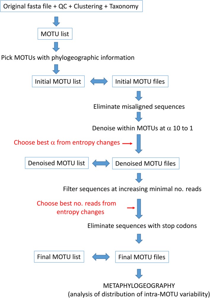
Schematic representation of the pipeline followed in this study. See Methods for details. The red arrows and text indicate the two steps in the pipeline where parameter selection should be carried out based on entropy values. MOTU, molecular operational taxonomic unit.

Finally, even if sequences retained were mostly correct, they can still include a number of nontarget variants due to heteroplasmy or numts (Elbrecht et al. 2018a). However, numts tend to accumulate mutations resulting in stop codons (Song et al. 2008). They can also present amino acid substitutions that result in a non‐functional protein: Pentinsaari et al. (2016) found 23 amino acids completely conserved across the COI barcode region in Metazoa, corresponding mostly to the helices of the protein that penetrate the mitochondrial membrane. Five of these amino acid positions occur in the fragment sequenced here. Some numts can therefore be detected by inspecting the sequences retained, as has been done in previous metabarcoding studies (Leray et al. 2013). As the data set included many different eukaryotic groups with different genetic codes, we adopted a conservative approach. For each MOTU, we tried the 20 genetic code variants stored in the Biostrings R package (Pagès et al. 2018) and used the translate function to obtain the corresponding amino acid sequence. We then chose, for each MOTU, the genetic code giving the lower number of stop codons (often several code variants resulted in no stop codons). In addition, we verified (for the metazoan MOTUs) that the five conserved positions described above did not have any amino acid substitution. The MOTUs denoised with the optimal α‐value (first step), once filtered with the optimal abundance cutoff (second step) were checked for the presence of stop codons and amino acid changes, and the sequences presenting them were removed from the data set. The remaining MOTUs and sequences constituted the curated data set for further analyses (Fig. 1).

Metaphylogeographic analyses

We performed network analyses with function HaploNet of the R package pegas (Paradis 2010). We used function amova of the R package ade4 (Dray and Dufour 2007) to compute analyses of molecular variance (AMOVA) in order to ascertain the percent variation associated with the hierarchical organization of the samples. For AMOVA, we used the proportion of the different sequences present (option distances = NULL). Preliminary assays considering also sequence distances (not just sequence frequencies) gave highly similar results and were computationally slower.

In these analyses, we needed to capture the quantitative information regarding frequencies of the different sequence variants. As mentioned above, using number of reads as a proxy for individual‐based abundances can be misleading. We adopted a semiquantitative index based on Wangensteen et al. (2018b) applied within each MOTU. To obtain this semiquantitative ranking, we ordered the sequences of each sample in each MOTU by increasing number of reads and ranked them from 0 to 4, indicating that the sequence is either absent in that sample (rank 0) or falls in the following percentiles of the distribution of ordered sequences: rank 1, ≤50%; rank 2, >50 ≤ 75%; rank 3, >75 ≤ 90%; rank 4, >90%. These semiquantitative ranks were used as proxies for haplotype abundances in the analyses.

Comparison with previous studies

After examination of the curated MOTU data set, we found only two species for which conventional phylogeographic analyses had been performed using COI information in the same geographic area: the sea urchin Paracentrotus lividus and the brittle star Ophiothrix fragilis.

For Paracentrotus lividus, we collated haplotype information from studies spanning the Atlanto‐Mediterranean transition (Duran et al. 2004), trimmed the sequences to the same fragment amplified in our study, and compared the haplotypes with the ones encountered in our metabarcoding data set. Duran et al. (2004) included two populations close to our localities: Eivissa Island in the Balearic Archipelago, and Ferrol in the Galician coast. Networks were generated with the haplotypes found in these localities and compared with our results.

For Ophiothrix fragilis, our MOTU corresponded to Lineage II of Pérez‐Portela et al. (2013). This brittle star is in fact a complex of species, and Lineage II is likely a cryptic species (Taboada and Pérez‐Portela 2016), but it remains unnamed so far. As before, we extracted haplotype information from all localities in Pérez‐Portela et al. (2013), spanning the Atlanto‐Mediterranean area, and compared with our results. We also obtained haplotype networks for the two closest populations studied in that work: Alcudia in the Balearic Archipelago and Ferrol in the Galician coast.

Results

The data set

The original data set, once quality and length filtered, contained 25,772,264 sequences of 8,900,080 unique sequences. Without singletons, the numbers were reduced to 17,808,524 reads and 936,340 unique sequences. Following the pipeline, we obtained a MOTU list of 26,561 eukaryote MOTUs. Of these, 13,410 MOTUs were present only in the Mediterranean site, 8,247 only in the Atlantic locality, and 4,904 were shared by both basins. Of the latter, only 722 MOTUs (with a total of 362,177 unique sequences and 9,430,236 reads) fulfilled the conditions that we set for the metaphylogeographic analyses (see Methods ) of having at least two sequences, being present in the two Parks with at least 20 reads in each one, and having appeared in the two years of study. After checking the alignment, only 158 sequences, comprising 689 reads, appeared as misaligned, mostly as a result of 1 bp slippage, and were removed. The singleton‐free fasta sequence file (paired, demultiplexed, and quality‐filtered), the original MOTU list, and the output of the SWARM analyses have been uploaded as a Mendeley data set (see Data Availability). The 722 MOTUs selected for the study are listed in Data S1, together with their taxonomic assignment and abundance (number of reads) per sample. The actual sequences of each MOTU, with their abundances per sample, are available at the Mendeley data set.

Simulation study

In our case, the top 1,000 sequences in the 722 MOTUs data set contained 5,948,135 reads. The entropy values of the codon positions of these sequences were: first position, 0.4298 ± 0.037 bits (mean ± SE); second position, 0.1833 ± 0.028 bits; third position, 0.9256 ± 0.023 bits. The simulation of increasing sequencing error rates clearly increased the entropy of the three positions (Fig. 2A), but more so for the less variable second position, which increased its value ~30% at the highest error rate. On the other hand, the third position increased entropy only about 1.8%. As a result, the entropy ratio (E _r, entropy2/entropy3) increased linearly with error rate, from 0.198 to 0.252 (Fig. 2B).

Figure 2.

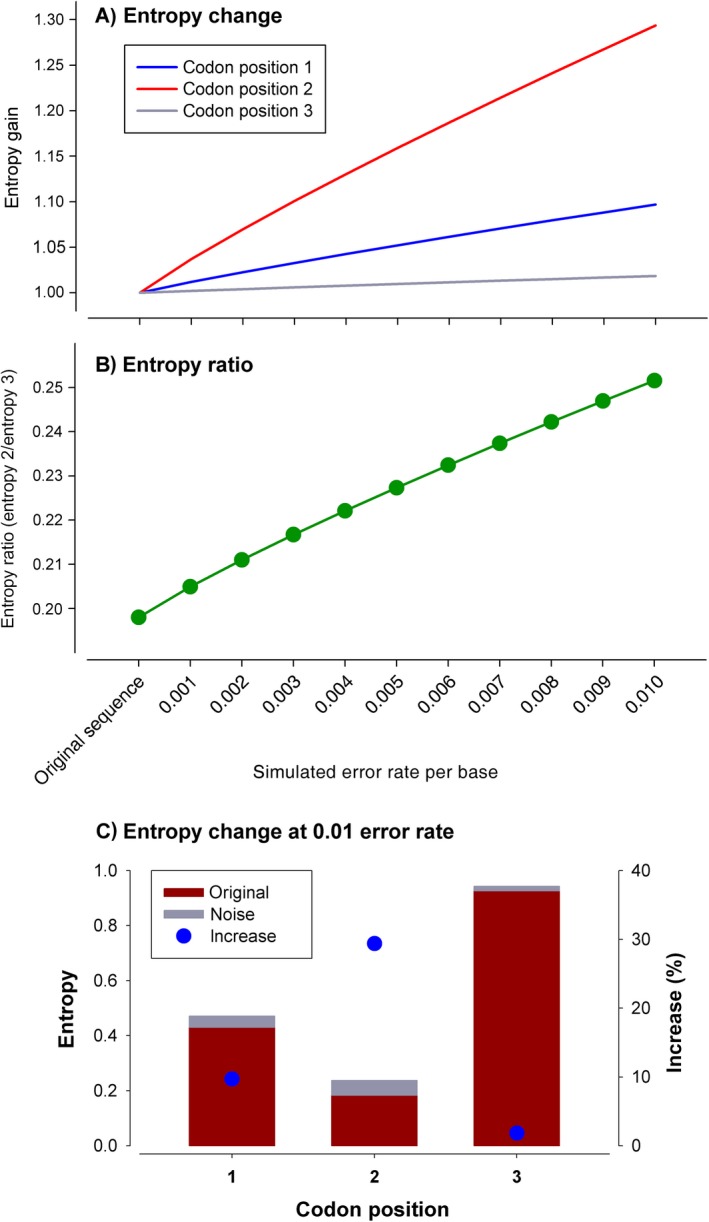
Simulation analysis. (A) Relative increase (initial value = 1) of the entropy values of each position at increased error rates. Bar plot shows the original and added entropy of each position at the highest (0.01) error rate. (B) Change in the entropy ratio. (C) Bar plot showing the original and added entropy of each position at the highest (0.01) error rate.

We then used the “noisy‐most” data set, the one simulated at the highest (0.01%) error rate. It had the same original number of reads, but 5,141,683 erroneous sequences (besides the 1,000 correct ones) were generated. For coherence with the global data set used, singletons were removed, leaving 144,791 sequences. This data set was then denoised at α values between 10 (least stringent) and 1 (most stringent). The E _r decreased drastically at the initial steps, concomitantly with a decrease in the number of erroneous sequences (Fig. 3A). The E _r value of the simulated data set reached the original value at α between 6 and 5. Taking the more conservative α = 5, which is also the point where the entropy curve levelled off (slope < 0.005), we found that the data set contained 895 of the original sequences and 17,799 erroneous sequences. In other words, while ~10% of the original sequences have been incorrectly merged, there remained still a high number of errors in the data set. Using only the denoise procedure, we got completely rid of erroneous sequences only at α = 1. But at this value only 66% of the correct sequences were retained.

Figure 3.

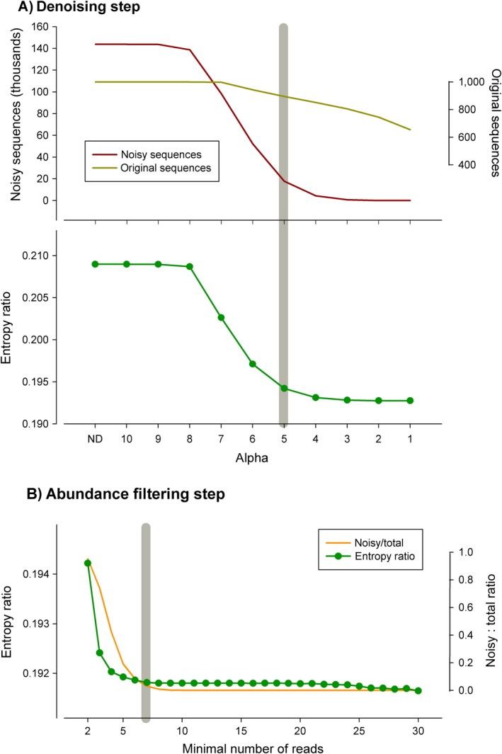
Simulation analysis. (A) Variation in the number of original and erroneous (“noisy”) sequences and entropy ratio at decreasing values of the alpha parameter of the denoising algorithm (ND, no denoising). (B) Change in the entropy ratio and in proportion of noisy vs. original sequences after filtering the data set by minimal abundance. The gray bars indicate the selected values of alpha (5) and minimal number of reads (7).

We therefore applied a round of filtering by minimal number of reads to the data set denoised at α = 5. Again, the E _r decreased sharply at increasing thresholds of minimal reads, following the elimination of erroneous sequences (Fig. 3B), and stabilized clearly at seven reads (Fig. 3B). The combination of denoising (α = 5) and filtering (minimal abundance = 7) allowed us to recover 924 sequences, of which 895 (97%) were among the 1,000 original sequences and only 3% were erroneous sequences. The frequency distribution of the number of reads in both the original (1,000) and the recovered (924) sequences was almost identical (not shown). Importantly, the shape of the E _r curve, specifically the stabilization points, proved informative to select the cut‐points for the two variables.

Data set cleaning

As a first step, we tried to identify PCR errors during amplification, as they can result in abundant sequences and be more difficult to spot. We assumed that PCR errors will affect one nucleotide at most, will occur in few samples, where they will coexist with the original sequence, and will be abundant. Therefore, we looked within the 722 MOTUs for sequences differing by one nucleotide from a more abundant one, co‐occurring always with it, being present in at most three samples (out of 51 samples), and having an abundance of >200 reads (set as a threshold to identify relatively abundant sequences). Only 14 such sequences were identified and merged with the more abundant ones.

After applying the denoising step for α values from 10 to 1 and a co‐occurrence index of 1 to the whole data set of 722 MOTUs, we examined the change in number of retained MOTUs and entropy ratio (Fig. 4A). The number of MOTUs remained constant but started decreasing at α = 6. As expected, the E _r decreased fast at first and more slowly at lower α‐values (i.e., with higher merging power) (Fig. 4A). The curve leveled off (slope below 0.005) at α = 5, with only a slight loss of MOTUs (six out of 722). We thus retained α = 5 as the optimal denoising parameter.

Figure 4.

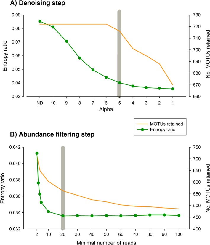
Final analyses of the littoral communities data set. (A) Variation in the number of sequences and number of MOTUs remaining at decreasing values of the alpha parameter (ND, no denoising) of the denoising algorithm. (B) Change in the entropy ratio and (C) change in residual (within‐sample) variance of the amova model. The gray bars indicate the selected alpha value (5) and abundance threshold (20).

The MOTU list corresponding to the denoised data set had 716 MOTUs, with 49,995 sequences (86% of the original sequences had been merged) and 9,426,339 reads (Data S1). The corresponding MOTU files (available at the Mendeley data set; see Data Availability) were submitted to an abundance filter, with a threshold from 2 to 100 reads. There was a decrease the number of MOTUs retained at increasing minimal numbers of reads, particularly in the interval 2–50 (Fig. 4B). The entropy ratio fell markedly and became stabilized at a value of 20 reads, after which it remained more or less constant (Fig. 4B). Thus, 20 reads was used as a minimal abundance threshold.

The sequences of the resulting MOTU files were translated and checked. Only eight sequences had stop codons, while a further 52 metazoan sequences had amino acid changes in the five positions invariable in Metazoa. These 60 sequences were eliminated, and the final MOTU list thus consisted of 563 MOTUs, with 7,146 sequences and 8,910,913 reads (Data S2). The final MOTU files were uploaded to the Mendeley data set (see Data Availability).

As for the taxonomy assigned, the most diverse groups of Eukarya in the final data set were Rhodophyta (91 MOTUs), Stramenopiles (90 MOTUs, mostly diatoms and brown algae), and Metazoa (273 MOTUs) (Data S2). A total of 99 eukaryotic MOTUs remained unassigned taxonomically (identified as Eukarya). Among metazoans, 112 MOTUs were assigned a species‐level taxon, while 225 MOTUs were assigned at least at the phylum level and 48 MOTUs remained unassigned (Data S2). The phyla of metazoans identified in the final MOTU list were Annelida (34 MOTUs), Arthropoda (56 MOTUs), Bryozoa (17 MOTUs), Chordata (eight MOTUs), Echinodermata (seven MOTUs), Mollusca (22 MOTUs), Nemertea (six MOTUs), Porifera (30 MOTUs), and Xenacoelomorpha (one MOTU).

Further analyses concentrated in the major groups detected, which accounted for 437 of the 464 MOTUs that could be assigned: red algae (Rhodophyta), diatoms (Bacillariophyta), brown algae (Phaeophyceae), and metazoans (Metazoa). In the latter, phylum‐level analyses were performed.

Phylogeography

Network graphs of the MOTUs (Appendix S2) showed different patterns, albeit in most cases one or a few haplotypes appeared as the most abundant, linked to a varying number of low abundance haplotypes. Some selected instances are presented in Fig. 5, showing also the change in network shape along the process of cleaning. It can be seen that the major pruning effect was due to the initial denoising step.

Figure 5.

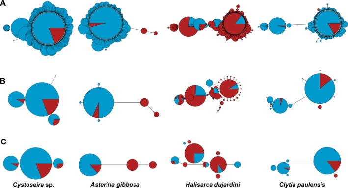
Selected instances of networks obtained at different stages of the pipeline: (A) without filters; (B) after denoising at alpha = 5; (C) after denoising at alpha = 5 plus minimal abundance filtering (threshold 20 reads). Circles represent haplotypes, and their diameters are proportional to their abundance (in semiquantitative ranks) in the samples. Blue color represent abundance in Mediterranean samples, red color in Atlantic samples. Length of links is proportional to the number of mutational steps between haplotypes. Note that circles in panels A, B, and C are not drawn to the same scale. The names correspond to the taxonomical identification of the MOTUs with ecotag (OBITools package). The MOTU ids (as per Data S1) are, from left to right, 143, 1740, 2500, and 25366.

AMOVAs were used to partition the genetic variance hierarchically into components due to the differences between seas, between communities within seas, between samples (replicates) within communities, and within samples. The average values of these variance components for the major groups detected, and for metazoan phyla separately, displayed a clear overall trend: genetic variance was concentrated within samples (60–75%) in all major groups (Fig. 6A). The other components of variance followed a decreasing trend, with a remarkable variance associated to differentiation between the two seas (14–25% of variance), and smaller variance between communities within each sea, and even lower between replicate samples of a given community. The latter component was almost negligible (<1.2%) in the non‐metazoan groups considered, but reached 5.4% in metazoans. The different components were compared across groups with ANOVA (followed by Student‐Newmann‐Keuls post hoc tests if significant). The between sample component was significantly higher (all P < 0.001) in metazoans than in the other groups. For the other components, the values were in general comparable, the only significant differences being a higher between seas differentiation in diatoms than in metazoans, and a higher within sample variance in red algae than in diatoms.

Figure 6.

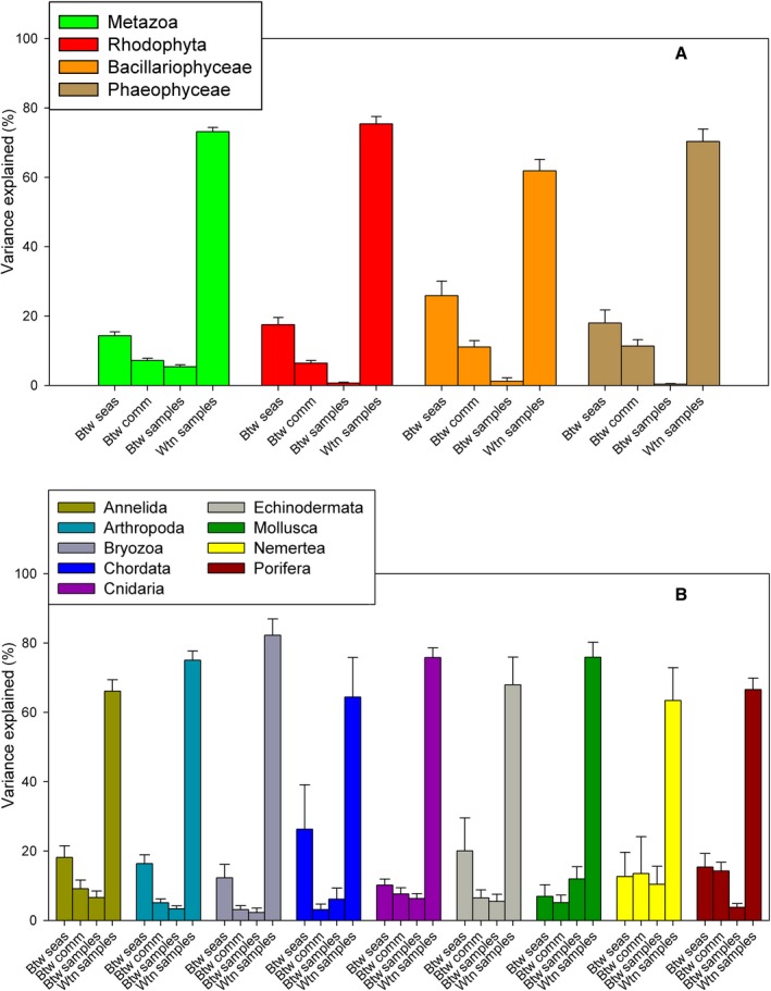
Summary of the mean percentage of variance explained by the hierarchical structure of the AMOVA: (A) as per eukaryote groups; (B) per metazoan phyla. Error bars are standard errors. Btw seas, between seas; btw comm, between communities within seas; btw samples, between samples within communities; wtn samples, within samples.

Metazoans therefore showed a higher heterogeneity between replicate samples of a given community than the other groups. When examined across phyla (Fig. 6B), albeit the overall trend was in general maintained, a dominant within sample component and a variance between seas > between communities > between samples, there were exceptions. In particular, molluscs had a high between sample variability, and other groups presented important small‐scale (between communities and/or between samples) variability as compared to the between seas differentiation (Cnidaria, Nemertea, Porifera). ANOVA showed few significant differences between phyla, the only significant comparisons involving the between samples component in molluscs, which was significantly higher than in bryozoans or sponges.

As for the comparison with previous studies, MOTU 697 was identified as the sea urchin Paracentrotus lividus with 100% sequence identity. This MOTU had 15 sequences. This species has an Atlanto‐Mediterranean distribution and Duran et al. (2004) analyzed populations spanning the western Mediterranean and northeast Atlantic with COI. In that work, 65 different haplotypes (of a longer fragment of COI) were detected. Once trimmed to our sequence length and collapsed, there were 32 remaining haplotypes. Nine out of the 15 sequences detected in our study had already been found by Duran and co‐workers, while the remaining six were new.

We then selected the haplotypes found in the previous work in the two localities closest to our sampling points (Eivissa in Balearic Islands and Ferrol in Galicia). There were 11 haplotypes (four of which were also present in our MOTU). We performed a network with the 2004 information and compared it with the one obtained for MOTU 697 with our semiquantitative abundance rank (Fig. 7A, B). The two networks had a similar shape, with a highest abundance of haplotype 2 (named after the order of abundance of sequences obtained for this MOTU), followed by haplotypes 1, 3, and 6. For the shared haplotypes, the between seas distribution was the same in the two studies (1, 2, and 3 shared between seas, six present only in the Atlantic). An AMOVA with a randomization test (n = 1,000) of our MOTU 697 revealed a significant differentiation between seas and between and within samples (P < 0.001) but not between communities (P = 0.812).

Figure 7.

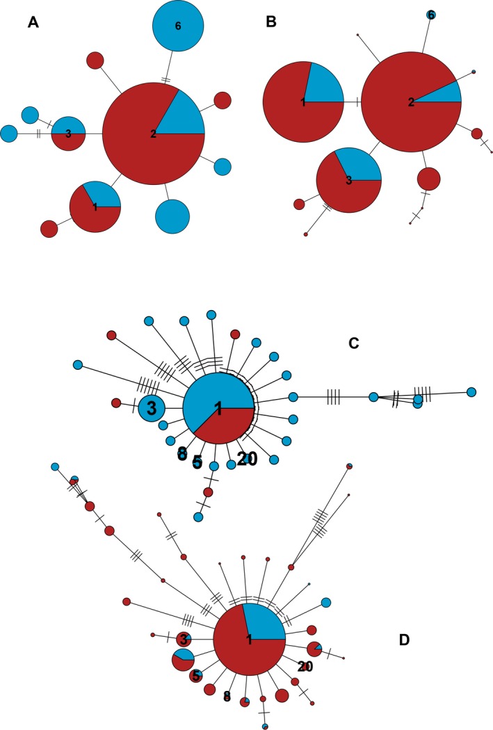
(A) Network constructed with the 11 haplotypes of the sea urchin Paracentrotus lividus found by Duran et al. (2004) in localities close to our sampling points and (B) network constructed with the 13 haplotypes comprising the MOTU corresponding to this species (id 697). Haplotypes common to both studies are numbered. (C) Network with the 29 haplotypes of the brittle star Ophiothrix fragilis identified by Pérez‐Portela et al. (2013) in localities close to our sampling points. (D) Network of the 34 haplotypes found in the present study in the MOTU corresponding to this species (id 15396). Haplotypes common to both studies are numbered. The short slashes in the links between haplotypes represent mutational steps. Colors as in Fig. 5.

The MOTU 15396, comprising 37 sequences, was identified (100% identity) with Ophiothrix sp. in Pérez‐Portela et al. (2013). In that work, the authors studied a controversial species complex of the genus Ophiothrix in the European waters using 16S and COI. Our sequences corresponded to the Lineage II of Ophiothrix fragilis in that work, that spanned from Britanny to Turkey. Pérez‐Portela et al. (2013) reported 125 haplotypes of Lineage II that, once trimmed to our 313 bp length, resulted in 90 different haplotypes. When merged with our data set, nine out of 37 sequences in MOTU 15396 had already been found in the previous study, while another 28 were new.

As before, we selected in Pérez‐Portela et al. (2013) the two localities closest to our sampling points (Alcudia in Balearic Islands, and Ferrol in Galicia). There were 29 haplotypes in these localities, of which five were shared with our study. The corresponding networks (Fig. 7C, D) showed a star‐shaped structure with a dominant haplotype 1 found in the two studies, with many low abundance sequences separated by one or a few mutations from the central haplotype and some longer branches. It is noteworthy that, in this case, the shared haplotypes do not have always the same inter‐basin distribution, thus, haplotype 1 was present in both oceans, but haplotypes 3, 8, and 5 present only in the Mediterranean site in the previous work, appeared now in the two seas (it should be noted that haplotype 3 did appear in other Atlantic sites in Pérez‐Portela et al. 2013). Finally, haplotype 20 was present only in the Mediterranean site in Pérez‐Portela et al. (2013) and only in the Atlantic locality in the present work. An AMOVA with a randomization test (n = 1,000) of our MOTU 15396 showed a significant component of variation related to between and within samples genetic variability (P < 0.001), but not between seas (P = 0.729) or between communities within seas (P = 0.212).

Discussion

In this study, we have developed a method to apply metabarcoding data sets to the study of intraspecies patterns of many species at a time using a highly variable coding fragment (COI). An initial denoising step, aimed at merging erroneous sequences with the correct ones, was followed by an abundance filtering step aimed at removing the remaining erroneous sequences. We used information from the variability of the different codon positions, following a simulation study, to select the best parameter values in the denoising and filtering steps. In addition, sample distribution information was used in the different steps to minimize loss of low abundance true sequences.

All cleaning procedures are a compromise between eliminating spurious sequences and losing true signal. In the benchmarking approach of Elbrecht et al. (2018a), 943 erroneous haplotypes appeared in a sample known to have only 15 before any processing. After a denoising process, 15 haplotypes remained but, of these, 6 (40%) were still sequences not present in the original sample, while 6 of the 15 original variants were discarded during the process. Clearly, separating wheat from chaff is a challenging problem.

In this study, we suggest an operational approach based on the stabilization of the entropy ratio to guide the cleaning procedures. Both the simulation approach and the analysis of the real data set pointed to an α‐value of 5 in the denoising step, which was also the optimal value selected in Elbrecht et al. (2018a). Whether this value can be taken as a general rule of thumb or not will require analyses of more data sets. For the filtering step, our method indicated 20 reads as the optimal threshold. This is a parameter that will likely vary between studies and should be optimized for each particular data set.

Some authors proposed that denoising should be performed before clustering to identify genuine sequence variants, using different procedures, such as the UNOISE2 algorithm that we have adapted here (Edgar 2016), the MED (minimum entropy decomposition; Eren et al. 2015) procedure, or the DADA2 algorithm (divisive amplicon denoising algorithm; Callahan et al. 2016). It has also been suggested that sequence variants should replace MOTUs to capture relevant biological variation (Edgar 2016, Callahan et al. 2017). This suggestion may be adequate in prokaryotes, where strains of the same species can have different characteristics (e.g., pathogenicity). However, for eukaryotes, and particularly metazoans, given the high amount of intraspecies information contained in the data sets, we think that it is more advisable to define meaningful MOTUs and perform denoising procedures within them, in order to obtain a “clean” data set and be able to use the intra‐MOTU sequence variability to make phylogeographic and population genetics inference. Clearly, our procedure is applicable only to coding sequences, which excludes much work done on protists based on ribosomal DNA. However, the growing number of metabarcoding studies using COI sequence data, together with the steady development of the BOLD database, makes us confident that many metabarcoding data sets of enormous potential for metaphylogeographic inference will become available in the near future.

We found a couple of instances of previous studies that have analysed COI structure in species recovered in our MOTU data set and in nearby localities. For Paracentrotus lividus, there were phylogeographic studies of the Atlanto‐Mediterranean area using COI (Duran et al. 2004), 16S (Calderón et al. 2008), and the nuclear ANT intron (Calderón et al. 2008). In all cases, a low, but significant, signal corresponding to the separation between Atlantic and Mediterranean was found. Our COI results were in agreement with those of Duran et al. (2004) for the localities that could be compared. We detected a somewhat higher number of haplotypes (11 in the previous work, 15 in our study) and the most common haplotypes were shared. The shape of the network was also similar. We want to emphasize that, as far as we could detect, not a single sea urchin of this species was present in our samples, so we obtained a similar level of haplotype diversity with community DNA than in a study specifically devoted to collect sea urchin specimens. For Ophiothrix fragilis, we also found a higher haplotype diversity (37 haplotypes) than in comparable localities in the work of Pérez‐Portela et al. (2013; 29 haplotypes). We identified five haplotypes that were shared in the two studies, including the commonest one in both data sets, and the networks again had similar structure. Of note here is that we could expand the distribution range of some of the haplotypes. Our AMOVA results for these two instances were equivalent to previous results for the only component that was analyzed in both studies (the between‐seas differentiation). Thus, Duran et al. (2004) found a significant (P < 0.05) between‐basin differentiation in Paracentrotus lividus, while Pérez‐Portela et al. (2013) did not find any significant genetic variability between Atlantic and Mediterranean for Lineage II of Ophiothrix fragilis (P = 0.790). This is consistent with our metabarcoding‐derived AMOVAs (P < 0.001 and P = 0.729, respectively). The two species are of remarkable ecological importance, Paracentrotus lividus is an engineer species able to modify the littoral landscape through its browsing activity (Palacin et al. 1998, Wangensteen et al. 2011), and is also a commercially exploited species (Barnes and Crook 2001). The different lineages of Ophiothrix fragilis are highly abundant components of the littoral communities and can form dense beds, with an important role in clearing particulate matter with their filtering activities (Davoult 1989, Davoult and Gounin 1995). For both species, therefore, an accurate assessment of the genetic relationships across the different basins is of utmost importance for conservation and management purposes.

We have used an already collected data set, which can mimic the situation that many a posteriori studies can encounter. However, future metabarcoding studies can be planned taking into consideration the potential application for intraspecies analyses as well. For instance, PCR replicates for each sample can be of tremendous advantage to eliminate noise in the first steps. Increasing ecological replication can also be of great value for metaphylogeographic studies. We strongly advocate that published metabarcoding studies include in their data sets the information about which sequences are grouped into each MOTU with their sample distribution. This information is not commonly provided, and is necessary to make these studies amenable for intraspecies and metaphylogeographic analyses.

Metabarcoding now occupies a well‐deserved prominent place among the methods for assessing community‐level diversity (Kelly et al. 2014, Adamowicz et al. 2019). We have shown that it can be also an important source for species‐level genetic diversity information for a wide assemblage of taxonomic groups. The mining of metabarcoding data for intraspecies information opens up a vast field with both basic and applied implications (Adams et al. 2019). Among the latter, the possibility of effectively basing conservation efforts on multispecies genetic metrics to preserve community‐level evolutionary patterns (Nielsen et al. 2017). It will also open the phylogeography field, nowadays restricted almost exclusively to macroorganisms, to the myriad of meio‐ and micro‐eukaryotes that make up most of the diversity present in natural communities.

Another related field is the assessment of connectivity between populations. This is important for endangered species, invasive species, protected areas design, and management in general. For instance, in the marine environment, differences in larval dispersal have often been suggested as responsible for determining population genetic structure, but other factors, such as variation in divergence times and changes in effective population sizes, must be taken into account (Hart and Marko 2010). A powerful test for these contrasting assumptions is to compare phylogeographic patterns among species that concur or differ in larval type. Metaphylogeography can provide such comparative data. For instance, in our study we have found that metazoans in general have more between‐replicate variability than other groups, and within metazoans the between community and between‐replicate components of genetic variation can be significantly different between phyla.

In conclusion, our study shows the feasibility of mining metabarcoding data sets for the analysis of intraspecies genetic diversity using objective parameters for denoising and filtering spurious sequences. We cannot at present advice a set pipeline to do this, as procedures should be customized for the particulars (e.g., replication level, number of habitats, number of localities) of each study data set. With this article, we hope to stir further discussion and developments in this field. The metaphylogeography application should be borne in mind to guide the planning and reporting of metabarcoding studies to ease the recovery of this, so far unexplored, vast amount of information.

Data Availability

Data are available on Mendeley Data at https://doi.org/10.17632/xpmtvn2k7m.2.

Supporting information

 

 

 

 

 

 

Turon X., Antich A., Palacín C., Præbel K., and Wangensteen O. S.. 2020. From metabarcoding to metaphylogeography: separating the wheat from the chaff. Ecological Applications 30(2):e02036 10.1002/eap.2036

Literature Cited

- Adamowicz, S. J. , et al. 2019. Trends in DNA barcoding and metabarcoding. Genome 62:5–8. [DOI] [PubMed] [Google Scholar]
- Adams, C. I. M. , Knapp M., Gemmell N. J., Jeunen G. J., Bunce M., Lamare M., and Taylor H. R.. 2019. Beyond diversity: can environmental DNA (eDNA) cur it as a population genetic tool? Genes 10:192. [DOI] [PMC free article] [PubMed] [Google Scholar]
- Andújar, C. , Arribas P., Yu D. W., Vogler A. P., and Emerson B. C.. 2018. Why the COI barcode should be the community DNA metabarcode for the Metazoa. Molecular Ecology 27:3968–3975. [DOI] [PubMed] [Google Scholar]
- Avise, J. C. 2009. Phylogeography: retrospect and prospect. Journal of Biogeography 36:3–15. [Google Scholar]
- Aylagas, E. , Borja A., Irigoien X., and Rodríguez‐Ezpeleta N.. 2016. Benchmarking DNA metabarcoding for biodiversity‐based monitoring and assessment. Frontiers in Marine Science 3:1–12. [Google Scholar]
- Baird, D. J. , and Hajibabaei M.. 2012. Biomonitoring 2.0: a new paradigm in ecosystem assessment made possible by next‐generation DNA sequencing. Molecular Ecology 21:2039–2044. [DOI] [PubMed] [Google Scholar]
- Baker, C. S. , Steel D., Nieukirk S., and Klinck H.. 2018. Environmental DNA (eDNA) from the wake of the whales: droplet digital PCR for detection and species identification. Frontiers in Marine Science 5:133. [Google Scholar]
- Barnes, D. K. A. , and Crook A. C.. 2001. Implications of temporal and spatial variability in Paracentrotus lividus populations to the associated commercial coastal fishery. Hydrobiologia 465:95–102. [Google Scholar]
- Bodenhofer, U. , Bonatesta E., Horejs‐Kainrath C., and Hochreiter S.. 2015. msa: an Rp ackage for multiple sequence alignment. Bioinformatics 31:3997–3999. [DOI] [PubMed] [Google Scholar]
- Bohmann, K. , Evans A., Gilbert M. T. P., Carvalho G. R., Creer S., Knapp M., Yu D. W., and de Bruyn M.. 2014. Environmental DNA for wildlife biology and biodiversity monitoring. Trends in Ecology and Evolution 29:358–367. [DOI] [PubMed] [Google Scholar]
- Boyer, F. , Mercier C., Bonin A., Le Bras Y., Taberlet P., and Coissac E.. 2016. OBITOOLS: a unix‐inspired software package for DNA metabarcoding. Molecular Ecology Resources 16:176–182. [DOI] [PubMed] [Google Scholar]
- Briski, E. , Ghabooli S., Bailey S. A., and MacIsaac H. J.. 2016. Are genetic databases sufficiently populated to detect non‐indigenous species? Biological Invasions 18:1911–1922. [DOI] [PMC free article] [PubMed] [Google Scholar]
- Calderón, I. , Giribet G., and Turon X.. 2008. Two markers and one history: phylogeography of the edible common sea urchin Paracentrotus lividus in the Lusitanian region. Marine Biology 154:137–151. [Google Scholar]
- Callahan, B. J. , McMurdie P. J., Rosen M. J., Han A. W., Johnson A. J. A., and Holmes S. P.. 2016. DADA2: High resolution sample inference from Illumina amplicon data. Nature Methods 13:581–583. [DOI] [PMC free article] [PubMed] [Google Scholar]
- Callahan, B. J. , McMurdie P. J., and Holmes S. P.. 2017. Exact sequence variants should replace operational taxonomic units in marker‐gene data analysis. ISME Journal 11:2639–2643. [DOI] [PMC free article] [PubMed] [Google Scholar]
- Cowart, D. A. , Pinheiro M., Mouchel O., Maguer M., Grall J., Miné J., and Arnaud‐Haond S.. 2015. Metabarcoding is powerful yet still blind: a comparative analysis of morphological and molecular surveys of seagrass communities. PLoS ONE 10:e0117562. [DOI] [PMC free article] [PubMed] [Google Scholar]
- Creer, S. , Deiner K., Frey S., Porazinska D., Taberlet P., Thomas K., Potter C., and Bik H.. 2016. The ecologist's field guide to sequence‐based identification of biodiversity. Methods in Ecology and Evolution 7:1008–1018. [Google Scholar]
- Dafforn, K. A. , Baird D. J., Chariton A. A., Sun M. Y., Brown M. V., Simpson S. L., Kelaher B. P., and Johnston E. M.. 2014. Faster, higher and stronger? the pros and cons of molecular faunal data for assessing ecosystem condition. Advances in Ecological Research 51:1–40. [Google Scholar]
- Davoult, D. 1989. Structure démografique et production de la population d'Ophiothrix fragilis (Abildgaard) du Détroit du Pas‐deCalais, France. Vie Marine 10:116–127. [Google Scholar]
- Davoult, D. , and Gounin F.. 1995. Suspension‐feeding activity of a dense Ophiothrix fragilis (Abildgaard) population at the water–sediment interface: time coupling of food availability and feeding behaviour of the species. Estuarine and Coastal Shelf Science 41:567–577. [Google Scholar]
- Deagle, B. E. , Jarman S. N., Coissac E., Pompanon F., and Taberlet P.. 2014. DNA metabarcoding and the cytochrome c oxidase subunit I marker: not a perfect match. Biology Letters 10:20140562. [DOI] [PMC free article] [PubMed] [Google Scholar]
- Deiner, K. , et al. 2017. Environmental DNA metabarcoding: transforming how we survey animal and plant communities. Molecular Ecology 26:5872–5895. [DOI] [PubMed] [Google Scholar]
- Dray, S. , and Dufour A.. 2007. The ade4 package: Implementing the duality diagram for ecologists. Journal of Statistical Software 22:1–20. [Google Scholar]
- Duran, S. , Palacín C., Becerro M. A., Turon X., and Giribet G.. 2004. Genetic diversity and population structure of the commercially harvested sea urchin Paracentrotus lividus (Echinodermata, Echinoidea). Molecular Ecology 13:3317–3328. [DOI] [PubMed] [Google Scholar]
- Edgar, R. C. 2016. UNOISE2: improved error‐correction for Illumina 16S and ITS amplicon sequencing. bioRxiv. 10.1101/081257 [DOI] [Google Scholar]
- Edgar, R. C. , and Flyvbjerg H.. 2015. Error filtering, pair assembly and error correction for next‐generation sequencing reads. Bioinformatics 31:3476–3482. [DOI] [PubMed] [Google Scholar]
- Elbrecht, V. , and Leese F.. 2015. Can DNA‐based ecosystem assessments quantify species abundance? Testing primer bias and biomass‐sequence relationships with an innovative metabarcoding protocol. PLoS ONE 10:e0130324. [DOI] [PMC free article] [PubMed] [Google Scholar]
- Elbrecht, V. , and Leese F.. 2017. Validation and development of COI metabarcoding primers for freshwater macroinvertebrate bioassessment. Frontiers in Environmental Science 5:11. [Google Scholar]
- Elbrecht, V. , Vamos E., Meissner K., Aroviita J., and Leese F.. 2017. Assessing strengths and weaknesses of DNA metabarcoding‐based macroinvertebrate identification for routine stream monitoring. Methods in Ecology and Evolution 8:1265–1275. [Google Scholar]
- Elbrecht, V. , Vamos E. E., Steinke D., and Leese F.. 2018a. Estimating intraspecific genetic diversity from community DNA metabarcoding data. PeerJ 6:e4644. [DOI] [PMC free article] [PubMed] [Google Scholar]
- Elbrecht, V. , Hebert P. D. N., and Steinke D.. 2018b. Slippage of degenerate primers can cause variation in amplicon length. Scientific Reports 8:10999. [DOI] [PMC free article] [PubMed] [Google Scholar]
- Emerson, B. C. , Cicconardi F., Fanciulli P. P., and Shaw P. J. A.. 2011. Phylogeny, phylogeography, phylobetadiversity and the molecular analysis of biological communities. Philosophical Transactions of the Royal Society B 366:2391–2402. [DOI] [PMC free article] [PubMed] [Google Scholar]
- Eren, A. M. , Morrison H. G., Lescault P. J., Reveillaud J., Vineis J. H., and Sogin M. L.. 2015. Minimum entropy decomposition: Unsupervised oligotyping for sensitive partitioning of high‐throughput marker gene sequences. ISME Journal 9:968–979. [DOI] [PMC free article] [PubMed] [Google Scholar]
- Ficetola, G. F. , et al. 2018. DNA from lake sediments reveals long‐term ecosystem changes after a biological invasion. Science Advances 4:eaar4292. [DOI] [PMC free article] [PubMed] [Google Scholar]
- Frøslev, T. G. , Kjoller R., Bruun H. H., Erjnaes R., Brundjerg A. K., Pietroni C., and Hansen A. J.. 2017. Algorithm for post‐clustering curation of DNA amplicon data yields reliable biodiversity estimates. Nature Communications 8:1188. [DOI] [PMC free article] [PubMed] [Google Scholar]
- González‐Tortuero, E. , Rusek J., Petrusek A., Giessler S., Lyras D., Grath S., Castro‐Monzón F., and Wolinska J.. 2015. The quantification of representative sequences pipeline for amplicon sequencing: case study on within‐population ITS1 sequence variation in a microparasite infecting Daphnia . Molecular Ecology Resources 15:1385–1395. [DOI] [PubMed] [Google Scholar]
- Gratton, P. , Marta S., Bocksberger G., Winter M., Trucchi E., and Kühl H.. 2017. A world of sequences: can we use georeferenced nucleotide databases for a robust automated phylogeography? Journal of Biogeography 44:475–486. [Google Scholar]
- Gunther, B. , Knebelsberger T., Neumann H., Laakmann S., and Martínez Arbizu P.. 2018. MEtabarcoding of marine environmental DNA based on mitochondrial and nuclear genes. Scientific Reports 8:14822. [DOI] [PMC free article] [PubMed] [Google Scholar]
- Hajibabaei, M. , Baird D. J., Fahnere N. A., Beiko R., and Golding G. B.. 2016. A new way to contemplate Darwin's tangled bank: how DNA barcodes are reconnecting biodiversity science and biomonitoring. Philosophical Transactions of the Royal Society B 371:20150330. [DOI] [PMC free article] [PubMed] [Google Scholar]
- Hart, M. W. , and Marko P. B.. 2010. It's about time: divergence, demography, and the evolution of developmental modes in marine invertebrates. Integrative and Comparative Biology 50:643–661. [DOI] [PubMed] [Google Scholar]
- Hausser, J. , and Strimmer K.. 2009. Entropy inference and the James‐Stein estimator, with application to nonlinear gene association networks. Journal of Machine Learning Research 10:1469–1484. [Google Scholar]
- Haye, P. A. , Segovia N. I., Muñoz‐Herrera N. C., Gálvez F. E., Martínez A., Meynard A., Pardo‐Gandarillas M. C., Poulin E., and Faugeron S.. 2014. Phylogeographic structure in benthic marine invertebrates of the Southern Pacific Coast of Chile with differing dispersal potential. PLoS ONE 9:e88613. [DOI] [PMC free article] [PubMed] [Google Scholar]
- Ji, Y. , et al. 2013. Reliable, verifiable and efficient monitoring of biodiversity via metabarcoding. Ecology Letters 16:1245–1257. [DOI] [PubMed] [Google Scholar]
- Kelly, R. P. , et al. 2014. Harnessing DNA to improve environmental management. Science 344:1455–1456. [DOI] [PubMed] [Google Scholar]
- Kemp, J. , López‐Baucells A., Rocha R., Wangensteen O. S., Andriatafika Z., Nair A., and Cabeza M.. 2019. Bats as potential suppressors of multiple agricultural pests: a case study from Madagascar. Agriculture, Ecosystems & Environment 269:88–96. [Google Scholar]
- Leray, M. , and Knowlton N.. 2015. DNA barcoding and metabarcoding of standardized samples reveal patterns of marine benthic diversity. Proceedings of the National Academy of Sciences USA 112:2076–2081. [DOI] [PMC free article] [PubMed] [Google Scholar]
- Leray, M. , and Knowlton N.. 2016. Censusing marine eukaryotic diversity in the twenty‐first century. Philosophical Transactions of the Royal Society B 371:20150331. [DOI] [PMC free article] [PubMed] [Google Scholar]
- Leray, M. , Yang J. Y., Meyer C. P., Mills S. C., Agudelo N., Ranwez V., Boehm J. T., and Machida R. J.. 2013. A new versatile primer set targeting a short fragment of the mitochondrial COI region for metabarcoding metazoan diversity: application for characterizing coral reef fish gut contents. Frontiers in Zoology 10:34. [DOI] [PMC free article] [PubMed] [Google Scholar]
- Macher, J. N. , Vivancos A., Piggott M. P., Centeno F. C., Matthaei C. D., and Leese F.. 2018. Comparison of environmental DNA and bulk‐sample metabarcoding using highly degenerate COI primers. Molecular Ecology Resources 18:1456–1468. [DOI] [PubMed] [Google Scholar]
- Macías‐Hernández, N. , Athey K., Tonzo V., Wangensteen O. S., Arnedo M. A., and Harwood J. D.. 2018. Molecular gut content analysis of different spider body parts. PLoS ONE 13:e0196589. [DOI] [PMC free article] [PubMed] [Google Scholar]
- Mahé, F. , Rognes T., Quince C., de Vargas C., and Dunthorn M.. 2015. Swarm v2: highly‐scalable and high‐resolution amplicon clustering. PeerJ 3:e1420. [DOI] [PMC free article] [PubMed] [Google Scholar]
- Nielsen, E. S. , Beger M., Henriques R., Selkoe K. A., and von der Heyden S.. 2017. Multispecies genetic objectives in spatial conservation planning. Conservation Biology 31:872–882. [DOI] [PubMed] [Google Scholar]
- Olesen, S. W. , Duvallet C., and Alm E. J.. 2017. dbOTU3: A new implementation of distribution‐based OTU calling. PLoS ONE 12:e0176335. [DOI] [PMC free article] [PubMed] [Google Scholar]
- Pagès, H. , Aboyoun P., Gentleman R., and DebRoy S.. 2018. Biostrings: Efficient manipulation of biological strings. R package version 2.50.1. https://bioconductor.org/packages/release/bioc/html/Biostrings.html
- Palacin, C. , Giribet G., Garner S., Dantart L., and Turon X.. 1998. Low densities of sea urchins influence the structure of algal assemblages in the western Mediterranean. Journal of Sea Research 39:281–290. [Google Scholar]
- Paradis, E. 2010. pegas: an R package for population genetics with an integrated‐modular approach. Bioinformatics 26:419–420. [DOI] [PubMed] [Google Scholar]
- Parsons, K. M. , Everett M., Dahlheim M., and Park L.. 2018. Water, water everywhere: environmental DNA can unlock population structure in elusive marine species. Royal Society Open Science 5:180537. [DOI] [PMC free article] [PubMed] [Google Scholar]
- Pascual, M. , Rives B., Schunter C., and Macpherson E.. 2017. Impact of life history traits on gene flow: A multispecies systematic review across oceanographic barriers in the Mediterranean Sea. PLoS ONE 12:e0176419. [DOI] [PMC free article] [PubMed] [Google Scholar]
- Pedro, P. M. , et al. 2017. Metabarcoding analyses enable differentiation of both interspecific assemblages and intraspecific divergence in habitats with differing management practices. Environmental Entomology 46:1381–1389. [DOI] [PubMed] [Google Scholar]
- Pentinsaari, M. , Salmela H., Mutanen M., and Roslin T.. 2016. Molecular evolution of a widely‐adopted taxonomic marker (COI) across the animal tree of life. Scientific Reports 6:35275. [DOI] [PMC free article] [PubMed] [Google Scholar]
- Pérez‐Portela, R. , Almada V., and Turon X.. 2013. Cryptic speciation and genetic structure of widely distributed brittle stars (Ophiuroidea) in Europe. Zoologica Scripta 42:151–169. [Google Scholar]
- Pfeiffer, F. , Gröber C., Blank M., Händler K., Beyer M., Schultze J. L., and Mayer G.. 2018. Systematic evaluation of error rates and causes in short samples in next‐generation sequencing. Scientific Reports 8:10950. [DOI] [PMC free article] [PubMed] [Google Scholar]
- Piñol, J. , Senar M. A., and Symondson O. C.. 2019. The choice of universal primers and the characteristics of the species mixture determines when DNA metabarcoding can be quantitative. Molecular Ecology 28:407–419. [DOI] [PubMed] [Google Scholar]
- Pochon, X. , Bott N. J., Smith K. F., and Wood S. A.. 2013. Evaluating detection limits of next‐generation sequencing for the surveillance and monitoring of international marine pest. PLoS ONE 8:e73935. [DOI] [PMC free article] [PubMed] [Google Scholar]
- Porter, T. M. , and Hajibabaei M.. 2018a. Automated high throughput animal CO1 metabarcode classification. Scientific Reports 8:4226. [DOI] [PMC free article] [PubMed] [Google Scholar]
- Porter, T. M. , and Hajibabaei M.. 2018b. Over 2.5 million COI sequences in GenBank and growing. PLoS ONE 13:e0200177. [DOI] [PMC free article] [PubMed] [Google Scholar]
- Porter, J. , and Zhang L.. 2017. InfoTrim: A DNA read quality trimmer using entropy. bioRxiv. 10.1101/201442 [DOI] [Google Scholar]
- R Development Core Team 2008. R: A language and environment for statistical computing. R Foundation for Statistical Computing, Vienna, Austria: http://www.R-project.org [Google Scholar]
- Ratnasingham, S. , and Hebert P. D. N.. 2007. bold: The Barcode of Life data system (http://www.barcodinglife.org). Molecular Ecology Notes 7:355–364. [DOI] [PMC free article] [PubMed] [Google Scholar]
- Rex, M. A. , and Ettter R. J.. 2010. Deep‐sea biodiversity. Pattern and scale. Harvard University Press, Cambridge, Massachusetts, USA. [Google Scholar]
- Rognes, T. , Flouri T., Nichols B., Quince C., and Mahé F. 2016. VSEARCH: a versatile open source tool for metagenomics. PeerJ 4:e0200177. [DOI] [PMC free article] [PubMed] [Google Scholar]
- Schirmer, M. , D'Amore R., Ijaz U. Z., Hall N., and Quince C.. 2016. Illumina error profiles: resolving fine‐scale variation in metagenomics sequencing data. BMC Bioinformatics 17:125. [DOI] [PMC free article] [PubMed] [Google Scholar]
- Schmidt, A. O. , and Herzel H.. 1997. Estimating the entropy of DNA sequences. Journal of Theoretical Biology 3:369–377. [DOI] [PubMed] [Google Scholar]
- Siegenthaler, A. , Wangensteen O. S., Benvenuto C., Campos J., and Mariani S.. 2019. DNA metabarcoding unveils multiscale trophic variation in a widespread coastal opportunist. Molecular Ecology 28:232–249. [DOI] [PMC free article] [PubMed] [Google Scholar]
- Sigsgaard, E. E. , et al. 2016. Population characteristics of a large whale shark aggregation inferred from seawater environmental DNA. Nature Ecology and Evolution 1:4. [DOI] [PubMed] [Google Scholar]
- Song, H. , Buhay J. E., Whiting M. F., and Crandall K. A.. 2008. Many species in one: DNA barcoding overestimates the number of species when nuclear mitochondrial pseudogenes are amplified. Proceedings of the National Academy of Sciences USA 105:13486–13491. [DOI] [PMC free article] [PubMed] [Google Scholar]
- Stat, M. , Huggett M. J., Bernasconi R., DiBattista J. D., Berry T. E., Newman S. J., Harvey E. S., and Bunce M.. 2017. Ecosystem monitoring with eDNA: metabarcoding across the tree of life in a tropical marine environment. Scientific Reports 7:12240. [DOI] [PMC free article] [PubMed] [Google Scholar]
- Stefanni, S. , Stankovic D., Borme D., De Olazabal A., Juretic T., Pallavicini A., and Tirelli V.. 2018. Multi‐marker metabarcoding approach to study mesozooplankton at basin scale. Scientific Reports 8:12085. [DOI] [PMC free article] [PubMed] [Google Scholar]
- Taberlet, P. , Bonin A., Zinger L., and Coissac E.. 2018. Environmental DNA for biodiversity research and monitoring. Oxford University Press, Oxford, UK. [Google Scholar]
- Taboada, S. , and Pérez‐Portela R.. 2016. Contrasted phylogeographic patterns on mitochondrial DNA of shallow and deep brittle stars across the Atlantic‐Mediterranean area. Scientific Reports 6:32425. [DOI] [PMC free article] [PubMed] [Google Scholar]
- Tang, C. Q. , Leasi F., Obertegger U., Kieneke A., Barraclough T. G., and Fontaneto D.. 2012. The widely used small subunit 18S rDNA molecule greatly underestimates true diversity in biodiversity surveys of the meiofauna. Proceedings of the National Academy of Sciences USA 109:16208–16212. [DOI] [PMC free article] [PubMed] [Google Scholar]
- Uchii, K. , Doi H., and Minamoto T.. 2016. A novel environmental DNA approach to quantify the cryptic invasion of non‐native genotypes. Molecular Ecology Resources 16:415‐422. [DOI] [PubMed] [Google Scholar]
- Vamos, E. E. , Elbrecht V., and Leese F.. 2017. Short COI markers for freshwater macroinvertebrate metabarcoding. Metabarcoding and Metagenomics 1:e14625. [Google Scholar]
- Vellend, M. , Lajoie G., Bourret A., Murria C., Kembel S. W., and Garant D.. 2014. Drawing ecological inferences from coincident patterns of population‐ and community‐level biodiversity. Molecular Ecology 23:2890–2901. [DOI] [PubMed] [Google Scholar]
- Wang, X. V. , Blanes N., Ding J., Sultana R., and Parmigiani G.. 2012. Estimation of sequencing error rates in short reads. BMC Bioinformatics 13:185. [DOI] [PMC free article] [PubMed] [Google Scholar]
- Wangensteen, O. S. and Turon X.. 2017. Metabarcoding techniques for assessing biodiversity of marine animal forests Pages 445–503 in Rossi S., Bramanti L., Gori A., and Orejas C., editors. Marine animal forests. The ecology of benthic biodiversity hotspots. Volume 1. Springer International Publishing, Switzerland. [Google Scholar]
- Wangensteen, O. S. , Turon X., Garcia‐Cisneros A., Recasens M., Romero J., and Palacin C.. 2011. A wolf in sheep's clothing: carnivory in dominant sea urchins in the Mediterranean. Marine Ecology Progress Series 441:117–128. [Google Scholar]
- Wangensteen, O. S. , Palacín C., Guardiola M., and Turon X.. 2018a. DNA metabarcoding of littoral hard‐bottom communities: high diversity and database gaps revealed by two molecular markers. Peer J 6:e4705. [DOI] [PMC free article] [PubMed] [Google Scholar]
- Wangensteen, O. S. , Cebrian E., Palacín C., and Turon X.. 2018b. Under the canopy: community‐wide effects of invasive algae in Marine Protected Areas revealed by metabarcoding. Marine Pollution Bulletin 127:54–66. [DOI] [PubMed] [Google Scholar]
- Wares, J. P. , and Pappalardo P.. 2016. Can theory improve the scope of quantitative metazoan metabarcoding? Diversity 8:1. [Google Scholar]
- Wheeler, Q. , Raven P. H., and Wilson E. O.. 2004. Taxonomy: impediment or expedient? Science 303:285. [DOI] [PubMed] [Google Scholar]
- Zink, R. M. 2002. Methods in comparative phylogeography, and their application to studying evolution in the North American aridlands. Integrative and Comparative Biology 42:953–959. [DOI] [PubMed] [Google Scholar]
Associated Data
This section collects any data citations, data availability statements, or supplementary materials included in this article.
Supplementary Materials
Data Availability Statement