Quantitative Analysis of Pedogenic Thresholds and Domains in Volcanic Soils

Abstract

Pedogenic thresholds describe where soil properties or processes change in an abrupt/nonlinear fashion in response to small changes in environmental forcing. Contrastingly, soil process domains refer to the space between thresholds where soil properties are either unchanged, or change gradually, across a broad range of environmental forcing. Here, we test quantitatively for the presence of thresholds in patterns of soil properties across a climatic gradient on soils developed from ~20 ky old basaltic substrate on the Island of Hawai’i. From multiple soil properties, we quantitatively identified a threshold at ~750 mm/y of water balance (precipitation minus potential evapotranspiration), delineating the upper water balance boundary of soil fertility in these soils. From the threshold in the ratio of exchangeable Ca to total Ca we identified the lower water balance boundary of soil fertility in these soils at −1000 mm/y, however this threshold was qualitatively described as it lies near the limit of the climate gradient data where the statistical approach can not be applied. These two results represent the first time that pedogenic thresholds have been identified using statistically rigorous methods and the limitations of said methods, respectively. Comparing the 20 ky soils to soils that developed on basaltic substrates of 1.2 ky, 7.5 ky, 150 ky, and 4100 ky in a time-climate matrix, we found that our quantitative analysis supports previous qualitatively identified thresholds in the soils developed from older substrates. We also identified the 20 ky as the transition from kinetic to supply limitation for plant nutrients in soil in this system.

Introduction

Water facilitates chemical reactions in soil, and water flux drives many of the functional properties in soil by redistributing or removing ions (Chadwick and Chorover 2001). Consequently the amount and timing of water inputs and losses by evapotranspiration and/or leaching are important determinants of ecosystem properties (Jenny 1980).

Evaluations of soil properties along rainfall gradients demonstrate that soil properties change abruptly over small changes in water balance (Chadwick and Chorover 2001; Ewing and others 2006; Dixon and Chadwick 2016). Reactions that buffer soils are particularly important, and several distinct buffering systems dominate across the soil pH range—from the carbonate equilibria in high-pH soils to weathering and cation exchange at intermediate pH to aluminum (Al) in acid soils (Chadwick and Chorover 2001; Slessarev and others 2016). When the capacity of one of these buffering systems is exceeded, a small change in water balance can cause an abrupt transition to a new set of chemical buffers. Abrupt transitions in soil properties along a gradient in environmental forcing are considered “pedogenic thresholds”, while the regions between thresholds where soil properties or processes change relatively little despite large differences in environmental forcing are termed “process domains” (Chadwick and Chorover 2001; Vitousek and Chadwick 2013). In addition to buffering, other processes such as redox dynamics and consequent iron (Fe) mobility can also create thresholds and domains (Miller and others 2001; Chacon and others 2006; Vitousek and Chadwick 2013).

The physical geography of the Hawaiian Islands provides an excellent time-climate matrix in which it is possible to evaluate the role of water balance in determining changes in soil properties. The northeast trade winds impinging on different age volcanoes create orographic changes in rainfall and rain-shadows that produce strong rainfall gradients over short distances (Giambelluca and others 2013). Soil sampling along these rainfall gradients on young (<10 ky) and older (~150 ky and ~4100 ky) substrates have been instrumental in identifying soil process domains and pedogenic thresholds (Chadwick and others 2003; Vitousek and Chadwick 2013; Lincoln and others 2014). Combined, the results from these studies show that substrate age is an important determinant of the rainfall where thresholds occur. For example, although every Hawai’i climate transect shows a threshold in the availability of rock-derived nutrient cations and in pH, this threshold occurs at different levels of rainfall on the various substrates—moving to increasingly lower rainfall as substrate age increases. Additionally, the mechanism behind these thresholds appears to be different between the younger and older substrates. On young substrates the threshold is controlled by kinetic limitations on the rate of mineral weathering. Whereas on old substrates the threshold appears to be driven by limitations on the supply of nutrients due to the irreversible depletion of weatherable minerals in the soil. (Vitousek and Chadwick 2013; Lincoln and others 2014).

Building upon these previous studies, in this paper we evaluate the control water balance exerts on soil properties along a rainfall gradient on an intermediate age (~20 ky) substrate on Mauna Kea Volcano, Hawai’i. We then describe a climate-age matrix combining our data and data from previous work on climate gradients in Hawai’i (Vitousek 2004; Vitousek and Chadwick 2013; Lincoln and others 2014) to investigate temporal shifts in thresholds and define the temporal transition from kinetic to supply limitation and how water balance controls the transition. To do this, we introduce a statistical approach to rigorously define meaningful nonlinear shifts in soil properties as a function of water balance. We use these statistically defined nonlinearities to identify pedogenic thresholds and soil process domains, adding quantitative analysis to the identification of pedogenic thresholds.

Methods

Hawai’i as a model system

Hawai’i provides an ideal setting to investigate questions of soil development: many of the factors that control soil development can either be held constant to a much greater extent than in continental settings (parent material chemistry, topography, and biological diversity) or vary in generally well defined and understood ways (climate and parent material age) (Jenny 1941; Chadwick and others 2003; Vitousek 2004; Vitousek and Chadwick 2013).

Soils in Hawai’i are derived from basaltic parent material from the hotspot volcanism that formed the islands, and consequently the chemical composition of parent material has lower variability than continental settings (Wolfe and others 1997; Duncan and others 1991). Additionally, constructional surfaces of the shield volcanoes support little topographic variation, and remnants of the constructional surfaces can be found even on the oldest islands (Vitousek 2004; Vitousek and Chadwick 2013). The biological diversity of the Hawaiian Archipelago is also much more constrained than in continental settings—due to the archipelagos extreme geographic isolation that makes species dispersal difficult (Vitousek 2004).

The climate in Hawai’i is primarily controlled by the topography of the islands. Rainfall is driven primarily by the interaction between island topography and the Northeast trade winds, while temperature varies predictably with elevation (Giambelluca 2013). Because of the topographic controls on climate, continuous gradients for both rainfall and temperature exist on all the islands. While the climate factors follow topographic patterns, lava flow and ash deposit (parent material) ages are well constrained, and vary nearly continuously from recent deposits to nearly 5 million years from southeast to northwest across the archipelago (Duncan and others 1991). In this way, parent material age can be held constant or varied by sampling soils derived from the same eruptive event or from different eruptive events, respectively (Wolfe and others 1997).

Site description

We collected soil samples along a transect across a precipitation gradient on the windward side of Mauna Kea on the Island of Hawai’i. Mean annual precipitation (MAP) varies from ~450 to ~5200 mm; mean annual temperature from ~6 to ~15 °C, and elevation from ~3520 to ~1220 m, with a negative relationship between both climate variables (precipitation and temperature) and elevation (Figure 1) (Giambelluca and others 2013).

Figure 1.

Climate variables across Mauna Kea. Mean annual precipitation (MAP) (filled blue circles), Priestley-Taylor potential evapotranspiration (PET) (open black circles), MAP-PET (that is, water balance; open blue circles), and mean annual air temperature (filled red circles).

In this paper, soil properties are displayed as a function of water balance—precipitation minus potential evapotranspiration (PET)—rather than rainfall. We used water balance because it more accurately describes the amount of water moving through the soil column, and thus affecting soil development. While rainfall measures the input of water into the system, it fails to capture gaseous losses (evapotranspiration). We used Priestley-Taylor PET as modeled by Giambelluca and others (2014), as it has been shown to accurately estimate PET across a broad range of temperatures and vegetation types (Stannard 1993; Sumner and Jacobs 2005). On the Mauna Kea gradient, PET ranges between ~1380 and ~1880 mm/y (Figure 1), and is positively correlated with elevation except for a break at ~1800 m that roughly aligns with the average height of the trade wind inversion (~1700 – 1900 m) (Ward and Galewsky 2014).

The soils we sampled developed on basaltic hawaiite and mugearite lava flows with thick ash layers overlaying these flows. The ages of this depositional sequence are between 65 and 14 ky (Wolfe and Morris 1996). As the soil sampled developed on top of the depositional sequence that occurred during this time period, and largely ended by 14 ky ago, we use a parent material age of 20 ky as a compromise between the 14 ky end date and the fact that not all areas of the mountain were likely covered by the youngest eruptions.

At low elevations along the transect, plant communities are dominated by a mix of bogs, patches dominated by the mat-forming fern Dicranopteris linearis, and scrub forest dominated by the native tree ‘Ōhi’a (Metrosideros polymorpha). At slightly higher elevation, plant composition transitions to a forest ecosystem dominated by Koa (Acacia koa) and ‘Ōhi’a (Mueller-Dombois 1987; Kraus 2012). This native forest gives way to introduced Eurasian pasture grasses between 1600 and 1800 m elevation. Māmane (Sophora chrysophylla) savannah is the dominant high elevation ecosystem, extending from ~2150 m up to the tree line at ~3050 m (Juvik and Juvik 1984). Between tree line and ~3320 m vegetation is sparse, but Pūkiawe (Styphelia tameiameiae) occurs in these sites. Above ~3320 m to the end of our gradient at ~3520 m, sampling sites lacked vascular plants.

Soil Sampling and Analysis

Across the transect we collected depth-integrated surface soil samples every 250 m (n = 97). For each of these samples we removed any litter or O horizon material. We then collected and homogenized the top 30 cm of mineral soil. We also described and sampled soils in 8 soil pits, dug to either a depth of >1 m or an impenetrable layer, at intervals of 1.5 – 2 km across the gradient (~300 m of elevation change). For each soil pit, we described the soil profile and collected samples from each horizon. To control for variations in relief, both types of samples were collected in the center of topographic high points to minimize the amount of erosional additions or losses associated with slopes and topographic low points. Soil classifications ranged from Xeric Vitricryands (unweathered to poorly weathered ash deposits) in the driest sites to Terric Haplohemists (high in organic matter at the surface transitioning to mineral soil at depth) in the wettest sites, and are presented in table 1.

Table 1. Site characteristics and classification of soil profiles.

Mean annual precipitation (MAP) and mean annual air temperature (MAAT) are taken from Giambelluca 2013 and 2014, respectively. NRCS SCAN stations at 2842 and 1949m were used in determining soil moisture and temperature regimes. We determined GFP11 & GFP10 to be cryic soils by their monthly air temperatures, and because they are colder than the 2842m station, which has soil temperatures on the colder end of the frigid range. We determined GFP11 & GFP10 to be xeric soils by their monthly rainfall, which shows the little rainfall they receive falls primarily in the winter. We determined GFP09 is an ustic soil by the 2842m station that has an ustic soil moisture regime and has similar rainfall and air temperatures. We determined GFP08 is an udic soil by rainfall data. The 1949m station has udic soil conditions, thus we determined all sites receiving similar or higher precipitations (≥~2200mm/yr), and were at lower elevations were also udic. We used the USDA Soil Survey to corroborate moisture and temperature regimes for all sites except GFP11 and GFP10, which lacked such information. Andic soil properties were determined by the sum of Al and 1/2Fe in acid ammonium oxalate extractions.

Water Balance	Elevation	MAP	MAAT	Vegetation	Soil
(mm/y)	(m)	(mm)	(°C)		Classification
−1190	3334	534	6	Barren	Xeric Vitricryand
−1240	3048	635	7	Pūkiawe, sparse	Xeric Vitricryand
−1100	2700	780	8	Māmane & Eurasian grasses	Typic Ustivitrand
−430	2435	1096	9	Eurasian grasses	Pachic Haplustand
100	2127	1578	10	Eurasian grasses	Histic Epiaquand
670	1831	2092	11	Eurasian grasses	Aquic Placudand
2000	1526	3479	13	Koa & ferns	Terric Haplohemist
4300	1246	5678	15	‘Ōhi’a & ferns	Terric Haplohemist

Once collected, we sieved all samples to 2 mm, separated them into four homogenous subsamples, and then air-dried them. One subsample was weighed, oven dried, and reweighed to calculate water content; the second was analyzed for resin extractable phosphorus (P), exchangeable Al, acid ammonium oxalate Fe and Al, total carbon (C), and total nitrogen (N) at Stanford University. We determined resin P by the anion exchange method described by Kuo (1996), using a WestCo SmartChem 200 discrete analyzer for the analyses. For exchangeable Al we used the 0.1 M BaCl₂ method. For C and N, we used a Carlo Erba NA 1500 analyzer. To determine if carbonates were present, a subsample of soil from sites with pH >6 was acid washed and reanalyzed for total C. No sites had detectable differences in total C between untreated and acid treated soils, so we assume that total C equals organic C for these soils. The third subsample was analyzed for pH, cation exchange capacity (CEC), base saturation, and exchangeable cations (calcium (Ca), potassium (K), sodium (Na), and magnesium (Mg)) at the University of California Santa Barbara using standard methods described in Chadwick and others (2003). The fourth subsample was sent to ALS Chemex (Reno, NV, USA) and analyzed for the total concentrations of 10 elements (Si, Al, Fe, Ca, Mg, Na, K, P, Ti, and Nb) via lithium borate fusion followed by x-ray fluorescence spectrometry.

Percent Remaining Calculation

Gains and losses of elements can be obscured by dilation or collapse of the soil volume (Brimhall and Dietrich 1987). To correct for these changes, we report elemental data as percent remaining relative to parent material using a minimally mobile index element and the equation (Kurtz and others 2000):

$$E_r= \left[\frac{\left(C_{E,s}/C_{I,s}\right)}{\left(C_{E,p}/C_{I,p}\right)}\right]\times 100$$

Where C represents the concentration of an element, E is the element of interest, and I is the index element (Niobium (Nb) in this case). The subscripts r, s, and p refer to percent remaining, the soil, and the parent material, respectively. Kurtz and others (2000) demonstrated that Nb (along with Ta) is the least mobile element in Hawaiian soils. Other studies have used Ti as an immobile reference element (Bullen and Chadwick 2016), and where Nb concentrations were below the detection limit we use Ti as the immobile reference element. We also tested the Ti/Nb approach described by Bullen and Chadwick (2016), and found no difference between estimates of gains and losses calculated using Ti and Nb for all elements except Fe. The calculation of Fe remaining is discussed below.

For parent material chemistry, we collected rock samples for chemical analyses—3 tephra samples from the two driest sites; 5 rock samples from a quarry located at ~1800 m (19.834N, 155.339W); and a gravel sample from the boundary between the bedrock and soil at the quarry site. Given the high rainfall, advanced state of weathering, and thick weathering profiles found in the wet sites, we were unable to collect unweathered parent material samples near the wet extreme of the gradient. Prior to analysis, weathering rinds were removed from the rocks, minimizing the impacts of chemical weathering on our estimates. Mauna Kea has experienced multiple eruptions and ash deposition events, and consequently it is possible that some parent material samples are from different events; however they are all derived from the final alkalic stage of Mauna Kea eruptions, and thus should share a similar chemistry (Wolfe and Morris 1996). The elemental data for the parent material are reported in table 2.

Table 2. Elemental composition of parent material for elements of interest.

Elemental percentages obtained via lithium borate fusion and XRF. Parent material chemistry is based on 9 samples—3 tephra samples, 2 bedrock samples, and 1 gravel sample from the bedrock soil interface.

	Si (%)	Al (%)	Fe (%)	P (%)	Ca (%)	Mg (%)	Na (%)	K (%)	Ti (%)	Nb (ppm)
Mean Value	22.61	9.14	8.51	0.40	4.94	2.45	3.40	1.46	1.73	60.44
Standard Deviation	0.76	0.23	0.32	0.02	0.21	0.16	0.26	0.26	0.11	1.59

To evaluate homogeneity of the parent material samples, we tested how correlated the samples chemical composition were using the Pearson correlation method. We assumed that two parent material samples are from the same parent material if they have a correlation coefficient >0.9 (Christopher Oze personal communication). While there was variation among the samples, all comparisons between samples had correlation coefficients of 0.99 or greater, indicating that the unweathered materials we sampled came from the same source. Additionally, as these samples are from the same stage of volcanism as the ash depositions, their chemistry should be comparable to that of the ash and thus representative of parent material values.

It is possible that our parent material samples did not represent the ash parent material’s chemistry, and thus would be unsuitable for the study even though they came from the same alkalic stage of volcanism. To test the suitability of the parent material selection and percent remaining calculations further, we used the methods described in Bullen and Chadwick (2016) as a secondary check. This method relies on the systematic relationships between Ti/Nb and the ratio of elements of interest to Nb in the parent material (i.e. C_E,p/C_I,p). This allowed us to test if our percent remaining calculations are sensitive to the parent material we chose.

As both Ti and Nb are considered immobile elements in soil, the ratio of Ti to Nb in the soil should be comparable to the ratio in said soil’s parent material. Thus, we were able to combine our known Ti to Nb ratios with previously collected data on Mauna Kea parent material geochemistry and identify chemistries of theoretical parent materials for each soil. From the previously collected parent material data from across Mauna Kea, in combination with parent material data we collected, we created linear models between Ti/Nb and C_E,p/Nb_I,p. We found strong relationships (p < 0.001 and R² > 0.85) between parent material Ti:Nb and Fe:Nb, Ca:Nb, and Mg:Nb. From these relationships, we calculated C_E,p/C_I,p for each soil sample we collected (for the elements Fe, Ca, and Mg), and subsequently a percent remaining for the applicable elements.

For all elements except Fe, we found no differences when comparing percent remaining calculated using the two methods. Consequently, for our study we presented the % remaining relative to parent material results using the collected parent material samples and not the Bullen and Chadwick (2016) method.

For Fe, based on the depth-distribution of calculated Fe for the full soil profiles we concluded that the Ti:Nb approach represents the more reasonable baseline for Fe dynamic here. Thus, we reported Ti:Nb calculated Fe percent remaining. For all other elemental comparisons we reported the percent remaining based on our collected parent material samples.

Statistical analyses

All statistical analyses were done using R (v3.0) or Microsoft Excel. We used segmented linear regressions (“Segmented” R package) to determine the existence and location of breakpoints in the patterns of different soil properties across the gradient (Muggeo 2003). For the breakpoint analysis the null hypothesis is that there are no breakpoints. As such, the analysis was first run blind without setting the number of potential breakpoints. If a breakpoint was found, we then tested to see if additional breakpoints improved the fit or not.

When breakpoints were identified, the significance of the nonlinearity in the regression was tested using the Davies’ Test (Davies 2002). We also report 95% confidence intervals for any breakpoints. Breakpoints are mathematically identifiable nonlinear patterns in a soil property, of which pedogenic thresholds are a subset. Our identification of pedogenic thresholds is based off of the interpretation of the statistically defined breakpoints.

Breakpoints represent locations that could either be pedogenic thresholds, or shifts in the relative strength of environmental factors. The pattern of resin P in Hawi soils illustrates this distinction; Vitousek and Chadwick (2013) report a peak in resin P at ~1200 mm/y MAP and a threshold at 2100 mm/y MAP. Both the peak and the threshold are identifiable breakpoints using segmented regression. However, the breakpoint at 2100 mm/y is a pedogenic threshold that represents the rainfall above which most rock-derived elements are depleted and there is no longer an enrichment of surface soils from deeper in the soil column via biological uplift (Jobbagy and Jackson 2004). In contrast, the peak at 1200 mm/y represents a breakpoint within a process domain; approaching this breakpoint from below, biological uplift is increasingly important in shaping surface soil P, while above it leaching increases in importance with increasing rainfall. However, the influence of biological uplift shapes soil properties on both flanks of the peak.

We used circular binary segmentation (“PSCBS” R package) to develop a breakpoint model of Ti:Nb across the rainfall gradient to identify potential parent material mixing (Olshen and others 2004). Circular binary segmentation is a statistical method first developed in genomics for identification of alterations to chromosomes, and works by splitting the data into two populations then testing for statistical differences between the population means. For the circular binary segmentations, a breakpoint is identified where a data split results in significant difference between the means on each side of the split. For our study, we used a significance level of 0.05.

For soil properties with heteroskedastic responses (Ti, total Fe, total P, and soil pH), we performed bootstrapped random sampling with replacement for calculating the segmented regressions and threshold bounds. The bootstrapped sample size was equal to the actual sample population size (n = 97) and the bootstrapped sampling was run 500 times for a given analysis. When bootstrap sampling was done, the threshold and confidence interval reported are the bootstrap means and are indicated by the subscript _Bootstrap.

Age comparison

To put the Mauna Kea gradient in context, we compare the dynamics of two important plant nutrients, Ca and P (total concentrations, percent remaining, and labile pools) along 5 climate gradients in Hawai’i that differ in substrate age, though are similar in parent material chemistry. Two of these gradients are on relatively young lava flows (1.2 and 7.5 ky) in the Kona District of Hawai’i Island (Lincoln and others, 2014); both cover much narrower water balance ranges (<1500 mm/y) than the other gradients. The Mauna Kea gradient was the next youngest on 20 ky substrate, followed by the Hawi gradient on 150 ky substrate and the Kauai gradient on 4100 ky substrate (Vitousek and Chadwick 2013). We used segmented linear regression analyses for each of the gradients to identify how pedogenic thresholds and process domains have shifted along these gradients as a function of substrate age (see Table 3 for thresholds and Table 4 for peaks). The relatively narrow climate ranges covered by the two Kona gradients precluded meaningful outcomes for many of the segmented analyses though we were still able to draw insights from the overall trends.

Table 3. Thresholds from rainfall gradients of different ages.

Thresholds in a given soil property. Values are mm of precipitation minus potential evapotranspiration on an annual basis, with the 95% confidence interval.

	Calcium			Phosphorus
Gradient	% Remaining	Total	Exchangeable	% Remaining	Total	Resin
Mauna Kea 20kyr	800±200	780±180	760±470	NA	1810±450	NA
Hawi 150ky	370±100	500±120	460±100	410±150	NA	150±130
Kauai 4100ky	−360±480	−500±470	−510±210	−20*	NA	−500±300

^*Threshold calculated using circular binary segmentation, which does not allow for calculation of the 95% confidence interval.

Table 4. Peaks in elemental pools from rainfall gradients of different ages.

Peaks in a given soil property. Values are mm of precipitation minus PET on an annual basis, with the 95% confidence interval.

	Calcium			Phosphorus
Gradient	% Remaining	Total	Exchangeable	% Remaining	Total	Resin
Kona 1.2kyr	−220±160	NA	NA	NA	NA	−370±130
Kona 7.5kyr	NA	NA	−420±210	NA	NA	NA
Mauna Kea 20kyr	NA	NA	−480±220	140±390	690±240	NA
Hawi 150ky	−180±90	−240±120	−360±80	−50±130	−190±530	−390±110

Results

We present patterns in a suite of soil properties from the 30 cm surface samples as a function of water balance.

Concentrations of Ti are negatively correlated with water balance below a water surplus of 210_Bootstrap ± 380 mm/y, and above that breakpoint they are positively correlated with water balance and become increasingly variable (Figure 2a). The pattern in Nb concentrations is qualitatively similar to that of Ti—negative in sites with water deficits and positive in sites with water surpluses (Figure 2a). However, Nb has no statistically significant breakpoint in its relationship with water balance. This is likely due to the high variability in Nb concentrations in the wetter sites. These patterns reflect increasing OM and hydration of soil minerals in progressively wetter sites (drier than the breakpoint), and progressively greater losses of mobile elements in wetter sites (Chadwick and others 2003).

Figure 2.

Ti and Nb in the surface 30 cm of soil on Mauna Kea substrate. A) Immobile element concentrations, Nb (red) and Ti (black), in soils. Solid vertical lines indicate the best estimate of the threshold in a given element calculated by segmented linear regression, whereas the dashed lines indicate the 95% confidence interval of the estimate. B) Ratio of Ti:Nb in 30 cm samples in soils on Mauna Kea. The horizontal red line is the average Ti:Nb for each region.

Soil Ti:Nb is not correlated with water balance, though it is significantly different in soils where water balance is <1190 mm/y (mean Ti:Nb = 290 ± 6) compared to soils where water balance is >1190 mm/y (mean Ti:Nb = 398 ± 39) (Figure 2b). The change in Ti:Nb implies an admixture of the parent material samples we collected from the high elevation dry sites with another source possessing a higher Ti:Nb. One possible source is volcanic ash from nearby Laupahoehoe age (65 – 4 kya) eruptions with mean Ti:Nb of 840 ± 80.

In combination, Si, Fe, and Al make up an average of 40.3% ± 0.2 of parent material (on a mass basis), with Si composing 22% ± 0.5 (Table 2). Across Mauna Kea, total Si (Figure 3a) and Si remaining (Figure 3b) are negatively correlated with water balance. Total Si and Si remaining have statistically indistinguishable breakpoints at water surpluses of 990 ± 200 mm/y and 1000 ± 280 mm/y, respectively, below which both decline sharply with increases in water balance. Above the breakpoints, the relationships are still negative, but significantly shallower.

Figure 3.

Si (black), Al (blue), and Fe (red) in the surface 30 cm of soil on Mauna Kea substrate; A) concentrations and B) percent remaining. Solid vertical lines indicate the best estimate of the threshold in a given element, whereas the dashed lines indicate the 95% confidence interval of the estimate (black for Si and red for Fe). Horizontal dashed line indicates 100% of the element remaining.

For Al (Figure 3a,b), total Al is negatively correlated with water balance (P < 0.0001), and there are no breakpoints across the gradient. The pattern is similar for Al remaining, although the slope of the relationship is steeper.

In contrast to Si and Al, Fe makes up a greater proportion of the soil as water balance increases (Figure 3a). In sites with water deficits greater than −80_Bootstrap ± 450 mm/y there is little variability in total Fe. Wetter than this breakpoint, total Fe is positively correlated with water balance. Fe remaining (Figure 3b) shows little deviation from 100% suggesting that there has been little Fe mobilization regardless of leaching power or redox processes that might be operative at higher water balances.

For the base cation data, only figures of Ca and Mg are presented in text; K and Na are in Figure 1 of the supplemental material. The total quantities of the base cations Ca, Mg, K, and Na decline rapidly within the upper 30 cm as water balance increases (Figure 4a). For all the base cations, there is a breakpoint where the steep decline transitions to a shallower decline with increasing water balance. Total Ca, K, and Na have statistically indistinguishable breakpoints, 780 ± 180, 630 ± 210, and 680 ± 190 mm/y, respectively. Total Mg has a significantly drier breakpoint at 30 ± 180 mm/y. The percent remaining for the base cations follow similar patterns as their total concentration (Figure 4b), with Mg, 240 ± 340 mm/y, having a drier breakpoint than Ca, K, and Na: 800 ± 200, 650 ± 230, and 720 ± 200 mm/y, respectively, though only the Mg and Ca breakpoints are significantly different.

Figure 4.

Divalent base cations in the surface 30 cm of soil on Mauna Kea substrate. A) Concentrations of Ca (open black circles) and Mg (red circles). B) Percent remaining of Ca (open black circles) and Mg (red circles). Horizontal dashed line indicates 100% of the element remaining. C Exchangeable Ca (open black circles) and Mg (red circles).

While the total pools of base cations are negatively correlated with water balance in these sites, the exchangeable pools are much more dynamic (Figure 4c). The most abundant exchangeable cation, Ca, is positively correlated with water balance to a peak (breakpoint) in soils with water deficits of −480 ± 220 mm/y and then declines to low values that persist into the wettest sites above water surpluses of 760 ± 470 mm/y. The pattern in exchangeable K is the same as that of exchangeable Ca, and exchangeable K’s two breakpoints, at −260 ± 250 and 680 ± 600 mm/y are statistically indistinguishable from Ca’s (Supplemental Figure 1). While Ca and K have two breakpoints, exchangeable Mg only has one at −498 ± 392 mm/y, not significantly different from the drier breakpoint of Ca and K. Below the breakpoint exchangeable Mg is positively correlated with water balance and above it is negatively correlated. Unlike the other exchangeable cations, Na does not vary significantly with water balance.

In the driest portion of the gradient, C and N concentrations are less than 1% and 0.1% respectively. Both C and N are positively correlated with water balance in sites drier than the breakpoints of 720 ± 300 and 550 ± 300 mm/y, for C and N respectively. In sites wetter than the respective breakpoint, C is uncorrelated with water balance and N is negatively correlated (Figure 5a). At the peak, C and N represent ~30% and 1% of dry soil mass. The soil C:N is positively correlated with water balance across the gradient, though there is a breakpoint at −1010 ± 170 mm/y (Figure 5b).

Figure 5.

A) C (open black circles) and N (red circles) in the surface 30 cm of soils on Mauna Kea substrate. B) C:N (open black circles), N:P (blue triangles), and C:P (red circles) in the surface 30 cm soils on Mauna Kea substrate.

Across the gradient total P is between 5 and 1.5 g/kg, and there are two breakpoints in its relationship to water balance: 690_Bootstrap ± 240 mm/y and 1810_Bootstrap ± 450 mm/y (Figure 6a). Between the two breakpoints, total P is negatively correlated with water balance. Contrastingly in sites drier than the dry breakpoint and wetter than the wet breakpoint, there is no relationship between total P and water balance. Both C:P and N:P are positively correlated with water balance, without a breakpoint (Figure 5b).

Figure 6.

P in the surface 30 cm of soil on Mauna Kea substrate. A) Percent remaining (open black circles) and concentration (red circles). B) Resin extractable P.

Labile (resin extractable) P concentrations are low across Mauna Kea (Figure 6b), even though more than half of the sites had >50% P remaining. Most sites (77%) have <1.0 mgP/kg soil in the upper 30 cm of soil. The remaining sites have resin P values below 5.5 mgP/kg soil, and we found no correlation between water balance and resin P.

Soil pH is negatively correlated with water balance with a breakpoint at 940_Bootstrap ± 610 mm/y (Figure 7a). In sites wetter than the breakpoint, the relationship is still negative, but significantly shallower (p < 0.001). In sites drier than the breakpoint, pH decreases from ~6.5 to ~4.5, and above the breakpoint pH continues to decrease to ~4.0.

Figure 7.

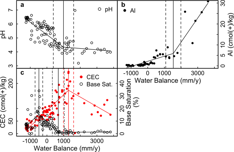
Select soil properties in surface 30 cm of soil on Mauna Kea substrate. A) pH, B) Exchangeable Al, C) Base saturation (open black circles) and CEC (red circles).

For exchangeable Al, sites with a water deficit have less than 0.5 cmol(+)/kg (Figure 7b). Qualitatively, once there is surplus water in the system, exchangeable Al increases to a plateau at 500 mm/y. This plateau persists until a statistically significant breakpoint at 1500 ± 460 mm/y, and in sites wetter than this breakpoint exchangeable Al increases rapidly with increasing water balance.

The cation exchange capacity (CEC) of soils is positively correlated with water balance up to a water surplus of 1300 ± 310 mm/y, and is negatively correlated above that breakpoint (Figure 7c). OM provides many of the exchange sites in these acidic soils, and therefore CEC is also positively correlated with soil C, though the relationship becomes weaker as %C increases. With high CEC and low base cation content of the soils on Mauna Kea, base saturation is low over most of the gradient (Figure 7c), with a peak value (breakpoint) of 35% at −480 ± 230 mm/y, and another breakpoint at 680 ± 360 mm/y. These breakpoints correspond to the breakpoints in exchangeable Ca and K.

Age Comparison

While thresholds and peaks are interpretations of the statistical breakpoints, for the age comparison results we use the terminology of thresholds and peaks. This is because the interpretation of what is a threshold was done in the previous studies, and our work here is applying a quantitative analysis for the locations of the peaks and thresholds.

For all Ca forms, Mauna Kea, Hawi, and Kauai have thresholds, above which the given form is very low in the soils (Table 3). Both the Mauna Kea and Hawi thresholds are in significantly (p < 0.05) wetter sites than the Kauai thresholds. The Mauna Kea thresholds are also in wetter sites than the Hawi thresholds, though only the threshold in Ca remaining is significantly different (p < 0.05). Given the short range of water balances covered by the Kona gradients, it is possible the gradients do not extend into the water balance where the threshold would exist.

Across all the gradients, except Kauai, Ca forms (exchangeable, total concentration, and percent remaining), have elevated levels in sites with water balance between −1000 and 0 (Supplementary Figure 2). The 7.5 ky Kona, Mauna Kea, and Hawi gradients have peaks in exchangeable Ca, and the 1.2 ky Kona and Hawi gradients have peaks in Ca remaining (Table 4). Unlike the thresholds in Ca, the breakpoints that represent peaks in Ca forms are not significantly different; though in all cases the Hawi peaks are in qualitatively wetter sites than the Kona and Mauna Kea peaks.

For total P, only Mauna Kea has a threshold in the relationship. This is possibly due to the Mauna Kea gradient extending into much wetter sites than other gradients (Supplementary Figure 3). Kauai and Hawi have thresholds in both P remaining and resin P (Table 3), and they are significantly (p < 0.05) wetter on the Hawi gradient.

The Hawi gradient has peaks in all forms of P, while peaks exist in total P and P remaining on Mauna Kea, and the 1.2 ky Kona gradient has a peak in resin P (Table 4). In cases where peaks are present, the Mauna Kea peaks are significantly (p < 0.05) wetter than the corresponding Hawi peak, and the 1.2 ky Kona peak in resin P is qualitatively wetter than the Hawi peak.

Discussion

Delineation of Soil Process domains

A cluster of breakpoints around 750 mm/y represents the threshold between soil process domains found on Mauna Kea. This threshold is the water balance at which the surface soils have been largely depleted of Si and base cations, and transition to very low (<5%) base saturation. In sites wetter than this threshold mobile elements, such as Si, Ca, and Mg, are nearly exhausted from the surface soils. It is also where soil N and P begin to decline in the surface soils. This cluster of thresholds represents the upper-bound (in terms of water balance) where biological uplift can maintain surface soils enriched with plant important nutrients on Mauna Kea and the exhaustion of primary minerals as a source for these nutrients in the soil matrix.

Wetter than the 750 mm/y threshold cluster is a soil domain of surface soils leached of base cations and Si. In this domain, we see the transition to soils where the supply of plant nutrients is limited by the depletion of weatherable primary minerals, inferred from the depletion of Si % remaining. The surface soils are predominantly composed of Fe, Al, and OM, while the pH buffering system has transitioned from weathering and the exchange of base cations and Al to a buffering system based on Al’s ability to hydrolyze water (Chadwick and Chorover 2001). Though Al secondary solid phases likely make up a substantial portion of soils in these sites, Al’s active role in the pH buffering system and the high leaching pressure in these sites results in Al mobilization and leaching losses from the surface 30 cm in these soils. Within this domain percent remaining of Al drops from >50% to <20%.

Drier than the 750 mm/y cluster is a soil domain where surface soils are enriched with rock derived nutrients, and buffered by mineral weathering and base cations. In this soil domain, N accumulates, and P is retained (and some sites show signs of biotic enrichment of P over 100% retention in surface soil). On Mauna Kea, this is the rainfall zone where biological uplift influences soil profiles, and there are sufficient water inputs to support mineral weathering and plant growth, but not enough water for leaching to deplete the surface soils over the ~20 ky of soil development. Dust inputs into the system are likely, however previous work found that dust provides minimal P and base cations to soils developing on substrate of this age (Chadwick and others 1999). In this domain, there are peaks in exchangeable Ca, K, and Mg, as well as base saturation that cluster around −400 mm/y of water balance and are statistically distinct from the thresholds that cluster around 750 mm/y. Unlike the other base cations, Na is a plant micronutrient, while Ca, Mg, and K are plant macronutrients. Consequently, the peak in exchangeable Ca, K, and Mg is missing from exchangeable Na, as the effects of biological uplift are not evident for Na (Jobbagy and Jackson 2001; Jobbagy and Jackson 2004). The cluster of peaks at −400 mm/y is where biological uplift has its greatest influence on Mauna Kea. It is also the point where the soils transition from ustic to udic conditions.

Sites in the driest portion of the <750 mm/y domain lack substantial plant cover, and consequently have little OM accumulation. Kramer and Chadwick (2016) showed that in similar sites weathering and secondary mineral development provided the means for C storage, but a lack of C inputs and water limitations prevented the OM accumulation normally associated with early stages of ecosystem development.

The soils in the driest portion of the <750 mm/y domain are similar to soils from the Kona gradients in that nutrient supplies are kinetically limited by the weathering of parent material rather than an absolute depletion of a given element in the soil column. The kinetic limitation on cation inputs results in low concentrations of base cations on exchange sites but high total concentrations and percent remaining relative to parent material.

The kinetic limitation on cation inputs is illustrated by the percentage of total Ca in the exchangeable pool (Figure 8). In sites with water balances less than −1000 mm/y exchangeable Ca represents <2% of total Ca, and then increases sharply in wetter sites to >10% of total Ca. The low percentage of total Ca in the exchangeable pool, combined with high Ca remaining in these very dry sites (Figure 4b), indicates that there are substantial amounts of Ca in the soil, but little has moved into the exchangeable pool. Moreover, the Ca that does move into the exchangeable pool is lost from the surface soils. Unfortunately, the statistical methods we applied to these data do not allow us to segregate this portion of the gradient from the broader <750 mm/y domain.

Figure 8.

Percentage of total Ca found as exchangeable Ca in the soil. Comparison is on a mass/mass basis.

Effect of Temperature-Rainfall Covariance

For other rainfall gradients that have been evaluated in Hawai’i, the climate goes from hot and dry to cool and wet (Vitousek and Chadwick 2013; Lincoln and others 2014). In contrast, the Mauna Kea gradient goes from cold and dry to warm and wet. For all the gradients, the highest calculated annual PET occurs in the lowest-rainfall sites; on other gradients this pattern is due to high temperature and low humidity in dry sites, while on Mauna Kea it is due to very dry air above the trade wind inversion. However, the cold dry sites on Mauna Kea have winter rains, lack vegetation, and have coarse textured soil (see Table 1). Consequently, pulsed rainfall or snow melt events are more likely to lead to leaching losses of water and nutrients on dry sites on Mauna Kea even though PET far exceeds MAP on an annual basis.

Pulsed rainfall events combined with a lack of vegetation likely explain the more acidic soils in dry sites of Mauna Kea in comparison to dry sites in Kona and on the Hawi gradient. As any Ca, Mg, K, and Na weathered from parent material are leached out of even the driest sites (and because CO₂ concentrations are low in pore water due to the absence of plants), conditions on Mauna Kea are not conducive for the production of pedogenic carbonates even in the driest sites (Kraimer and others 2005; Breecker and others 2009). By contrast, pedogenic carbonates are found in the vegetated dry sites on Hawi substrates receiving <700 mm/yr MAP (Vitousek and Chadwick 2013).

Age comparison

From the thresholds in the rock-derived, plant-important nutrients Ca and P we delineated pedogenic thresholds and soil process domains for the three oldest of the five climate gradients (Figure 9). The mineral depletion thresholds are based on the statistically defined breakpoints, and for the Hawi and Kauai gradients they are consistent with previous work identifying climate driven pedogenic thresholds and domains on these gradients with qualitative methods (Vitousek and Chadwick 2013).

Figure 9.

Pedogenic thresholds and soil process domains (color coded and labeled on figure) for the five water balance gradients. Due to the narrow water balance ranges the Kona gradients cover (1.2 and 7.5 ky on figure) we were unable to identify thresholds on these gradients. However, given the peaks in Ca and P identified on these gradients we believe the soils on these gradients are within the weathering and biological uplift domain (yellow with black striping). We identified three different thresholds across the gradients: the lower limit of detectable biological uplift (dotted vertical line); the depletion of primary minerals in the surface soils (solid vertical line); and the onset of low redox potentials in the soil (dashed vertical line).

The thresholds in the lower limit of water balance where biological uplift is detectable on the Mauna Kea and Hawi gradients are based on qualitative interpretation of the data due to limitations of our statistical approach. At the boundary of the data there is insufficient data on the boundary side of the breakpoint to produce a linear regression for comparison in the breakpoint analysis.

Given the relatively narrow climate ranges covered by the two Kona gradients we were unable to identify thresholds using segmented analyses. However, based on the peaks in Ca and P forms in these two gradients (Table 4) we believe that the Kona climate gradients cover the mineral weathering and biological uplift domain.

The Kauai thresholds occur at significantly lower water balances than those on the other gradients (Table 3), and in general Kauai soils are the most depleted in Ca and P (Supplementary Figures 2 and 3) for a given water balance. This follows a logical conceptual model, as Kauai is the gradient with the oldest substrate the soils have experienced the greatest total volume of water passing through them among our study sites (Hotchkiss and others 2000). This results in greater translocation of soil nutrients and thus the most depleted soils among our study sites.

While the Kauai thresholds are significantly drier, the large errors on the threshold estimates on the Mauna Kea and Hawi gradients mean they are statistically indistinguishable (Table 3), except for the threshold in Ca remaining. Qualitatively all the Mauna Kea thresholds occur in sites with more positive water balances than those on Hawi substrates, as would be expected for soils developing from younger substrate.

In addition to thresholds located in significantly drier regions, Kauai has a soil process domain in sites with water balances >880 mm/y that is delineated by a threshold of low redox potential and defined by soils with high C:N and the mobilization of Fe from the surface 30 cm. We, like Vitousek and Chadwick (2013), used the ratio of total Al to total Fe to identify this threshold and domain. Neither the Hawi nor the Mauna Kea gradient contains this domain, indicating that a considerable length of time is needed for this domain to develop.

Where the Kauai gradient contains a wetter threshold and domain, both Mauna Kea and Hawi have domains at the dry end of each gradient delineated by thresholds based on the driest point of detectable biological uplift. While these dry domains are both characterized by low concentrations of biologically available Ca and P, different soil processes dominate each domain: wind erosion on the Hawi gradient (Vitousek and Chadwick 2013) and kinetic limitations on mineral weathering on the Mauna Kea gradient. The difference in the dominant soil process is likely due to a lack of vegetation in the domain on Mauna Kea. Soils in the Hawi domain are depleted in all forms of Ca, which is consistent with wind erosion losses that erased the imprint of previous enrichment from biological uplift (Vitousek and Chadwick 2013). In contrast, the Mauna Kea soils are only low in exchangeable Ca, indicating that there has been no weathering or uplift in the soil.

As with the thresholds, when present, the position of the peaks in soil properties on Mauna Kea, Hawi, and the Kona gradients (though not the magnitude of enrichment in element pools) are not significantly different, save for the peaks in total P. However, the peaks in Ca remaining, exchangeable Ca, and Resin P occurred in qualitatively drier locations on the Kona gradients than the Hawi gradient. This shift is likely driven by the difference in parent material texture: soils on the Kona gradient are derived from coarse a’a lava flows compared to ash deposits on the Hawi gradient (Vitousek and Chadwick 2013; Lincoln and others 2014). In the coarse a’a material, elements that are released from the parent material due to weathering are easily lost from the system with rainfall due to a lack of adsorption sites and water holding materials. Our results support Lincoln and others’ (2014) conclusion that the depletion of rock-derived nutrients is shifted to drier sites on the Kona gradients than would be expected from the parent materials age.

A caveat to these comparisons is the accuracy of the rainfall and PET models on which we base our water balance values. Different models varied in their predictions of rainfall and PET values in some parts of Hawai’i (Giambelluca and others 1986; 2013). Additionally, Marshall and others (2017) found differences between modeled rainfall averages and measured averages (using years 1990 – 2007) on the leeward side of Kohala. As such, intra-gradient comparisons may be hampered by the limitations of the data sources we used.

For water balances between approximately −1000 and 0 mm/y, the magnitude of enrichment in Ca and P on the Hawi and Kona gradients is much greater than the enrichment seen on Mauna Kea. We see this in all P forms, in exchangeable Ca, and to a lesser extent Ca remaining. The pattern implies that this region of Mauna Kea experiences greater losses than the other gradients, or Hawi and Kona receive greater inputs of Ca and P to surface soils than Mauna Kea. In this region of the Mauna Kea gradient it is unlikely that pulse losses play a disproportionate role in leaching elements as sites in this region are vegetated, and both rainfall and transpiration are well distributed throughout the year (Giambelluca and others 2013; Giambelluca and others 2014).

Potential inputs include differences in biological uplift, or marine-aerosol-derived inputs for Ca. We can eliminate ocean inputs, as we found no increase in Na concentrations in the Hawi and Kona soils that would also result from ocean inputs. However, it is possible that differences in biological uplift, driven by temperature, play a role. The Mauna Kea sites in this rainfall zone are ~700m above comparable Hawi sites, and the highest Kona sites, with mean annual temperature ranging between 6–9°C cooler than Hawi sites. Because temperature affects the productivity of plants (Churkina and Running 1998; Gough and others 2008), lower temperatures could lead to lower primary productivity and consequently lower rates of biological uplift.

Conclusions

We identified two distinct clusters of breakpoints in soil properties (−400 and 750mm/yr of water balance). These breakpoints mark the peak in biological uplifts influence on surface soils and the upper bound (in water balance) of high soil fertility; the latter represents a widespread pedogenic threshold. Qualitatively we identify another possible threshold at −1000 mm/y that corresponds to the lower limit in water balance for the detection of biological uplift.

We also found evidence to support the belief that this age substrate contains the transition from kinetic to supply limitation on soil development, with the driest portion of the gradient likely limited by kinetic processes, and the wettest portion of the gradient controlled by the irreversible depletion of weatherable materials.

Across the climate-age matrix of the Hawaiian rainfall gradients, we identified statistically significant breakpoints in all gradients, and significant thresholds in the three oldest gradients (Kauai, Hawi, and Mauna Kea). Our results corroborate the conclusions of Lincoln and others (2014) that soil properties were shifted to drier positions on the coarse-grained Kona gradients. While we expected the fine-grained soils of Mauna Kea to have peaks and thresholds that were significantly wetter than Hawi, we found that the estimates were statistically indistinguishable—though all the thresholds and all peaks, save for the peak in %P remaining, are qualitative wetter on the Mauna Kea gradient than the Hawi gradient.

Manuscript Highlights.

• –We explore the climatic controls on soil biogeochemistry with novel statistical methods.
• –We found evidence for two thresholds in the dominant soil processes.
• –The location of these thresholds is dependent on the age of the soil’s parent material.

References

- Breecker DO, Sharp ZD, McFadden LD. 2009. Seasonal bias in the formation and stable isotopic composition of pedogenic carbonate in modern soils from central New Mexico, USA. Geological Society of America Bulletin 121:630–40. [Google Scholar]
- Brimhall GH, Dietrich WE. 1987. Constitutive mass balance relations between chemical composition, volume, density, porosity, and strain in metasomatic hydrochemical systems: Results on weathering and pedogenesis. Chemical Geology 51:567–87. [Google Scholar]
- Bullen T, Chadwick O. 2016. Ca, Sr and Ba stable isotopes reveal the fate of soil nutrients along a tropical climosequence in Hawaii. Chemical Geology 422:25–45. [Google Scholar]
- Chacon N, Silver WL, Dubinsky EA, Cusack DF. 2006. Iron reduction and soil phosphorus solubilization in humid tropical forests soils: the roles of labile carbon pools and an electron shuttle compound. Biogeochemistry 78:67–84. [Google Scholar]
- Chadwick OA, Derry LA, Vitousek PM, Huebert BJ, Hedin LO. 1999. Changing sources of nutrients during four million years of ecosystem development. Nature 397:491–497. [Google Scholar]
- Chadwick OA, Chorover J. 2001. The chemistry of pedogenic thresholds. Geoderma 100:321–53. [Google Scholar]
- Chadwick OA, Gavenda RT, Kelly EF, Ziegler K. 2003. The impact of climate on the biogeochemical functioning of volcanic soils. Chemical Geology 202:195–223. [Google Scholar]
- Churkina G, Running SW. 1998. Contrasting Climatic Controls on the Estimated Productivity of Global Terrestrial Biomes. Oecologia 1:206–15. [Google Scholar]
- Davies RB. 2002. Hypothesis Testing When a Nuisance Parameter Is Present Only under the Alternative: Linear Model Case. Biometrika 89:484–9. [Google Scholar]
- Dixon JL, Chadwick OA, Vitousek PM. 2016. Climate‐driven thresholds for chemical weathering in postglacial soils of New Zealand. Journal of Geophysical Research: Earth Surface. [Google Scholar]
- Duncan RA, Richards MA. 1991. Hotspots, mantle plumes, flood basalts, and true polar wander. Reviews of Geophysics. [Google Scholar]
- Ewing SA, Sutter B, Owen J, Nishiizumi K, Sharp W, Cliff SS, Perry K, Dietrich W, McKay CP, Amundson R. 2006. A threshold in soil formation at Earth’s arid–hyperarid transition. Geochimica Et Cosmochimica Acta 70:5293–322. [Google Scholar]
- Giambelluca TW, Chen Q, Frazier AG, Price JP, Chen Y-L, Chu P-S, Eischeid JK, and Delparte DM, 2013: Online Rainfall Atlas of Hawai’i. Bulletin of American Meteorological Society 94, 313–316, doi: 10.1175/BAMS-D-11-00228.1. [DOI] [Google Scholar]
- Giambelluca TW, Nullet MA, Schroeder TA. 1986. Rainfall Atlas of Hawai’i. [Google Scholar]
- Giambelluca TW, Shuai X, Barnes ML, Alliss RJ, Longman RJ, Miura T, Chen Q, Frazier AG, Mudd RG, Cuo L, and Businger AD. 2014. Evapotranspiration of Hawai’i. Final report submitted to the U.S. Army Corps of Engineers—Honolulu District, and the Commission on Water Resource Management, State of Hawai’i. [Google Scholar]
- Gough CM, Vogel CS, Schmid HP. 2008. Controls on annual forest carbon storage: lessons from the past and predictions for the future. BioScience 58:609–622. [Google Scholar]
- Hotchkiss S, Vitousek PM, Chadwick OA, Price J. 2000. Climate Cycles, Geomorphological Change, and the Interpretation of Soil and Ecosystem Development. Ecosystems 3:522–33. [Google Scholar]
- Jenny H 1980. The soil resource: origin and behavior. New York (NY):Springer-Verlag. [Google Scholar]
- Jobbagy EG, Jackson RB. 2001. The distribution of soil nutrients with depth: Global patterns and the imprint of plants. Biogeochemistry 53:51–77. [Google Scholar]
- Jobbagy EG, Jackson RB. 2004. The uplift of soil nutrients by plants: Biogeochemical consequences across scales. Ecology 85:2380–2389. [Google Scholar]
- Juvik JO, Juvik SP. 1984. Mauna Kea and the myth of multiple use: endangered species and mountain management in Hawaii. Mountain Research and Development:191–202. [Google Scholar]
- Kraimer RA, Monger HC, Steiner RL. 2005. Mineralogical Distinctions of Carbonates in Desert Soils. Soil Science Society of America Journal 69:1773. [Google Scholar]
- Kramer MG, Chadwick OA. 2016. Controls on carbon storage and weathering in volcanic soils across a high‐elevation climate gradient on Mauna Kea, Hawaii. Ecology 97:2384–95. [DOI] [PubMed] [Google Scholar]
- Kraus J, editor. 2012. Hakalau National Wildlife Refuge. U.S. Fish & Wildlife Service; http://www.fws.gov/hakalauforest/. Last accessed 2013 [Google Scholar]
- Kuo S 1996. Phosphorus Sparks DL, Page AL, Helmke PA, Loeppert RH, editors. Methods of Soil Analysis. Part 3 - Chemical Methods. Madison, WI: Soil Science Society of America; p869–919. [Google Scholar]
- Kurtz AC, Derry LA, Chadwick OA, Alfano MJ. 2000. Refractory element mobility in volcanic soils. Geology 28:683–6. [Google Scholar]
- Lincoln N, Chadwick O, Vitousek PM. 2014. Indicators of soil fertility and opportunities for precontact agriculture in Kona, Hawai’i. Ecosphere 5:1–20. [Google Scholar]
- Marshall K, Koseff C, Roberts A, Lindsey A, Kagawa AK, Lincoln N, Vitousek PM. 2017. Restoring people and productivity to Puanui: challenges and opportunities in the restoration of an intensive rain-fed Hawaiian field system. Ecology and Society 22:23. [Google Scholar]
- Miller A, Schuur E, Chadwick OA. 2001. Redox control of phosphorus pools in Hawaiian montane forest soils. Geoderma 102:219–37. [Google Scholar]
- Mueller-Dombois D 1987. Forest dynamics in Hawaii. Trends in Ecology & Evolution 2:216–220. [DOI] [PubMed] [Google Scholar]
- Muggeo VMR. 2003. Estimating regression models with unknown break‐points. Statistics in Medicine 22:3055–71. [DOI] [PubMed] [Google Scholar]
- Olshen AB, Venkatraman ES, Lucito R, Wigler M. 2004. Circular binary segmentation for the analysis of array‐based DNA copy number data. Biostatistics 5:557–72. [DOI] [PubMed] [Google Scholar]
- Slessarev EW, Lin Y, Bingham NL, Johnson JE, Dai Y. 2016. Water balance creates a threshold in soil pH at the global scale. Nature 540. [DOI] [PubMed] [Google Scholar]
- Stannard DI. 1993. Comparison of Penman‐Monteith, Shuttleworth‐Wallace, and modified Priestley‐Taylor evapotranspiration models for wildland vegetation in semiarid rangeland. Water Resources Research 29:1379–1392. [Google Scholar]
- Sumner DM, Jacobs JM. 2005. Utility of Penman–Monteith, Priestley–Taylor, reference evapotranspiration, and pan evaporation methods to estimate pasture evapotranspiration. Journal of Hydrology 308:81–104. [Google Scholar]
- Vitousek PM, Chadwick OA. 2013. Pedogenic Thresholds and Soil Process Domains in Basalt-Derived Soils. Ecosystems 16:1379–1395. [Google Scholar]
- Vitousek PM. 2004. Nutrient cycling and limitation: Hawai’i as a model system. Princeton (NJ): Princeton University Press. [Google Scholar]
- Ward DJ, Galewsky J. 2014. Exploring landscape sensitivity to the Pacific Trade Wind Inversion on the subsiding island of Hawaii. Biological Reviews 119:2048–69. [Google Scholar]
- Wolfe EW, Morris J. 1996. Geologic map of the island of Hawaii. Miscellaneous Investigations Series. [Google Scholar]
- Wolfe EW, Wise SW, Dalrymple GB. 1997. The geology and petrology of Mauna Kea Volcano, Hawaii–A study of post shield volcanism. U.S. Geological Survey. [Google Scholar]
Associated Data
This section collects any data citations, data availability statements, or supplementary materials included in this article.