Epidemiological implications of mobility between a large urban centre and smaller satellite cities

Abstract

An SIR infectious disease propagation model is considered that incorporates mobility of individuals between a large urban centre and smaller satellite cities. Because of the difference in population sizes, the urban centre has standard incidence and satellite cities have mass action incidence. It is shown that the general basic reproduction number ${\mathcal{R}}_0$ acts as a threshold between global asymptotic stability of the disease free equilibrium and disease persistence. The case of Winnipeg (MB, Canada) and some neighbouring satellite communities is then considered numerically to complement the mathematical analysis, highlighting the importance of taking into account not only ${\mathcal{R}}_0$ but also other measures of disease severity. It is found that the large urban centre governs most of the behaviour of the general system and control of the spread is better achieved by targeting it rather than reducing movement between the units. Also, the capacity of a satellite city to affect the general system depends on its population size and its connectivity to the main urban centre.

Introduction

With progress in technology, mobility, defined here very generally as consisting of all processes through which individuals change their location, has become more and more prevalent and easy. Among the consequences of this acceleration and generalization of mobility is a great speeding up and easing of the spatio-temporal spread of infectious diseases, as evidenced notably by the 2003 SARS epidemic or the 2009 H1N1 pandemic (Khan et al. 2009).

Studying the effect of mobility on the spread of an infectious disease can be accomplished in many ways, illustrating that the term mobility encompasses a wide variety of processes taking place on vastly different timescales. One of these methods are so-called metapopulation models, which consider distinct spatial locations called patches. In each patch, an epidemic model describes the spread of an infectious disease among members of the local population. The locations are then coupled in a graph, with the patches as vertices and arcs representing the possibility for individuals in the various epidemiological states to travel between locations.

Many aspects have been investigated in metapopulation models; see, e.g., the review by Arino (2009). One aspect that has not been the object of much attention is the effect of the interconnection of patches with very different population sizes on the dynamics of disease propagation in the coupled system. Wang and Zhao (2008) consider a model for two patches with periodic coefficients of infection and movement rates. Fromont et al. (2003) consider Feline Leukemia Virus in a metapopulation of cats living either in farms or in villages. In these papers, the authors consider coupled patches with some having mass action incidence and others with standard incidence.

In the same spirit, a metapopulation model for the spread of infection within cities is used here to study the movement of people between an urban centre and neighbouring satellite cities and the effect this has on the spatial and temporal spread of the disease. Large cities are indeed often associated to smaller cities of two main types. Suburban areas are most of the time very close to the major city. They can have distinct administrative structures, but a large fraction of their inhabitants commute to the large city (or to other suburban areas) during the work week, if not every day. They also often offer some of the amenities of the large city, such as shopping centres or recreational areas, so inhabitants of the latter also visit them regularly. They are difficult to distinguish from the large city and from a modelling perspective, the large city and its suburbs can generally be considered as a single unit. The other type of structures peripheral to a large urban area are so-called satellite cities. These are generally cities in their own right, located further away from the main city than are suburban areas. However, they are connected to the main city in many ways. For instance, while they generally have hospitals, these facilities are often able to deal only with general cases, with severe cases having to be treated in the large city’s facilities. Although not as closely integrated as a major city and suburban cities, individuals make regular movements between the locations.

An SIR-type metapopulation model is formulated, with standard incidence in the large urban centre and mass action incidence in the satellite cities, to tackle the following questions:

1. From Arino (2009) and other work on the subject, it appears that most of the time, the linear autonomous coupling of a collection of patches that are identical, save perhaps for parameter values, does not lead to behaviours that are more complex than those observed for the models in isolation. On the other hand, a change of incidence function within a single population can lead to complicated dynamics; see, e.g., Arino and McCluskey (2010). Does the coupling of patches with different incidence functions affect the dynamics of a metapopulation disease transmission model?

2. From a more practical point of view, urban centre and satellite cities systems abound. In such configurations, what drives disease propagation in the entire system? Can satellite cities “infect” the urban centre, can they protect themselves from infection by the urban centre? Does the size of a city play a role in its vulnerability to invasion by an infectious disease or its role in facilitating the spread of this disease?

Some mathematical analysis is conducted. Then the model is specialized numerically to several cities in the province of Manitoba (Canada): Winnipeg, the capital and largest urban centre with about 700,000 inhabitants, and satellite cities located some distance from Winnipeg.

Modelling

Assumptions

In each city, the population is divided between susceptible (S), infectious (I) and recovered (R) individuals, depending on their epidemiological status. The simple SIR formalism allows to capture the main characteristics of disease propagation without the burden of additional equations and parameters. Further, this allows to focus on the effect of size, since the behaviour of a classical SIR metapopulation model without size effects is well understood.

The large city is labelled with the numerical application to Winnipeg in mind: it is identified with the index $W$. There are a fixed small number $n$ of satellite cities, labelled $1,\dots ,n$. It is assumed that there is no movement between the smaller cities. This is, to a large extent, a reasonable assumption in the application considered; see Sect. 4. The mathematical analysis is not any more complicated if movement between the satellite cities is added to the model, it is omitted here for simplicity and because of the application considered. All individuals move at the same rate regardless of their epidemiological status. This simplification stems from the short distances involved.

The specificity of the model lies in the assumption that, depending on the size of the population in patches, different types of incidence functions are present (Fig. 1). There is a lot of debate about the nature of incidence functions (McCallum et al. 2001) and the interpretation that follows is by no means the only one possible. Here, as in the work of Arino and McCluskey (2010), it is assumed that mass action incidence is appropriate for smaller populations, while standard (or proportional) incidence better fits larger communities. Since the communities are much smaller than the urban centre, the nature of contacts is different. In the smaller communities, it is quite conceivable that an inhabitant can meet any other inhabitant, which is well described by a mass action incidence function. On the other hand, a large urban centre has several major shopping areas, numerous neighbourhoods, etc. Many inhabitants spend their days in a small number of neighbourhoods, rarely if ever visiting others. This situation is better reproduced by a proportional incidence function.

Fig. 1.

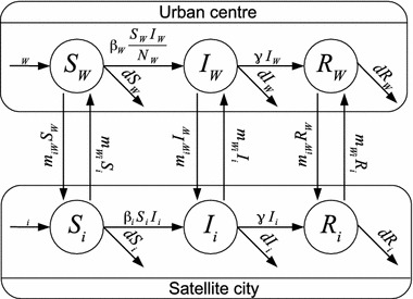
Flow diagram of the system. Represented here are the urban centre and one satellite city

The model and its parameters

The model consists of $3(n+1)$ differential equations. Those for the urban centre are given by

$$\begin{array}{cc}\hfill S_W^{\prime }& =b_W-{\mathit{\beta }}_W\frac{S_W{I}_W}{N_W}-d{S}_W+\sum _{i=1}^n{m}_{Wi}{S}_i-S_W\sum _{i=1}^n{m}_{iW}\hfill \end{array}$$ 1a

$$\begin{array}{cc}\hfill I_W^{\prime }& ={\mathit{\beta }}_W\frac{S_W{I}_W}{N_W}-\mathit{\gamma }{I}_W-d{I}_W+\sum _{i=1}^n{m}_{Wi}{I}_i-I_W\sum _{i=1}^n{m}_{iW}\hfill \end{array}$$ 1b

$$\begin{array}{cc}\hfill R_W^{\prime }& =\mathit{\gamma }{I}_W-d{R}_W+\sum _{i=1}^n{m}_{Wi}{R}_i-R_W\sum _{i=1}^n{m}_{iW},\hfill \end{array}$$ 1c

while equations for the satellite cities take the form, for $i=1,\dots ,n$,

$$\begin{array}{cc}\hfill S_i^{\prime }& =b_i-{\mathit{\beta }}_i{S}_i{I}_i-d{S}_i+m_{iW}{S}_W-m_{Wi}{S}_i\hfill \end{array}$$ 1d

$$\begin{array}{cc}\hfill I_i^{\prime }& ={\mathit{\beta }}_i{S}_i{I}_i-\mathit{\gamma }{I}_i-d{I}_i+m_{iW}{I}_W-m_{Wi}{I}_i\hfill \end{array}$$ 1e

$$\begin{array}{cc}\hfill R_i^{\prime }& =\mathit{\gamma }{I}_i-d{R}_i+m_{iW}{R}_W-m_{Wi}{R}_i.\hfill \end{array}$$ 1f

Here and throughout the remainder of the text, the index $x\in \{W,1,\dots ,n\}$ is used to alleviate notation; when referring to a city, “city $x$” refers to any of the urban centre or the smaller cities.

The parameter ${\mathit{\beta }}_x$ is the transmission coefficient in city $x$; it has units per unit time and per unit time per individual in $W$ and $i=1,\dots ,n$ and represents the rate of infection and the rate of infection per individual, respectively. The parameter $\mathit{\gamma }$ is the per capita rate of recovery, i.e., $1/\mathit{\gamma }$ is the mean of the exponentially distributed time of sojourn of individuals in the infectious class. The constant $b_x$ is the birth rate in city $x$ and $d$ is the per capita death rate. The rates of recovery and death are equal in all cities because sanitary conditions are comparable in the cities considered. The birth rate is allowed to differ between locations as it is used to set the equilibrium value of the population in the locations (see below). The parameter $m_{Wi}$ is the rate of movement from satellite city $i=1,\dots ,n$ to the urban centre, while $m_{iW}$ is the rate of movement from the urban centre to satellite city $i=1,\dots ,n$. Unless otherwise indicated, the rates of movement are positive. All other parameters are positive.

The total population in city $x$ is $N_x=S_x+I_x+R_x$. This number is assumed to be large compared to the number $n$ of cities considered, so that an ordinary differential equations approach is justified. System (1) is considered with nonnegative initial conditions such that $N(0)=N_W(0)+{\sum }_{i=1}^n{N}_i(0)>0$. To avoid dealing with a trivial case, it is also generally assumed that $I_W(0)+{\sum }_{i=1}^n{I}_i(0)>0$.

Mathematical analysis

Preliminaries

Summing all equations in (1) and denoting $N={\sum }_x{N}_x$ and $b={\sum }_x{b}_x$, the total population in the system is governed by

$$\begin{array}{c}\hfill N^{\prime }=b-dN,\end{array}$$

so the total population in the system tends to $b/d$ as $t\to \infty$. It is easy to verify that the positive orthant ${\mathbb{R}}^{3(n+1)}$ is invariant under the flow of (1), so all state variables are nonnegative and bounded.

Some notation will be useful for the remainder of the analysis. If $\mathbf{k}$ is a vector, the notation $\mathbf{k}\ge 0$ indicates that $\mathbf{k}$ has all its entries nonnegative, $\mathbf{k}>0$ means that $\mathbf{k}\ge 0$ with at least one positive entry; finally, $\mathbf{k}\gg 0$ means that $\mathbf{k}$ is entry-wise positive. The same notation is used for matrices. The analysis will also make use of the movement matrix, which is defined as

$$\begin{array}{c}\hfill \mathcal{M}=\left(\begin{array}{ccccc}-{\sum }_{i=1}^n{m}_{iW}& m_{W1}& m_{W2}& \cdots & m_{Wn}\\ m_{1W}& -m_{W1}& 0& \cdots & 0\\ m_{2W}& 0& -m_{W2}& & 0\\ & & \ddots & \ddots & \\ m_{nW}& 0& 0& & -m_{Wn}\end{array}\right).\end{array}$$ 2

Some properties of $\mathcal{M}$ will be used later on and are summarized in the following result.

Lemma 1

Let $c\in {\mathbb{R}}_{+}\backslash \{0\}$. The matrix $\mathcal{M}$ defined by (2) has the following properties.

• (i). $-\mathcal{M}$ is a singular M-matrix and has all its eigenvalues with nonpositive real parts.
• (ii). $-(\mathcal{M}-c\mathbb{I})$ is a nonsingular M-matrix.
• (iii). $-{(\mathcal{M}-c\mathbb{I})}^{-1}>0$.
• (iv). $\mathcal{M}-c\mathbb{I}$ has all its eigenvalues with real parts less than or equal to $-c$.
• (v).If $m_{Wi}>0$ and $m_{iW}>0$ for all $i=1,\dots ,n$, then $\mathcal{M},-\mathcal{M},\mathcal{M}-c\mathbb{I}$ and $-(\mathcal{M}-c\mathbb{I})$ are irreducible and $-{(\mathcal{M}-c\mathbb{I})}^{-1}\gg 0$.

Proof

(1) follows from Theorem 2 in the paper by Arino (2009). Since $-\mathcal{M}$ is an M-matrix, Lemma 6.4.1 in the book by Berman and Plemmons (1994) implies that, for $c>0,-\mathcal{M}+c\mathbb{I}$ is a nonsingular M-matrix, proving (2). Since $-(\mathcal{M}-c\mathbb{I})$ is a nonsingular M-matrix, Theorem 6.2.3.${\text{N}}_{38}$ in Berman and Plemmons (1994) gives (3). (4) Follows from Exercise 1.2.P8 in the book by Horn and Johnson (2013). Irreducibility of $\mathcal{M}$ in (5) comes from considering the directed graph (digraph) $\mathcal{G}(\mathcal{M})$ associated to $\mathcal{M}$, where $\mathcal{G}(\mathcal{M})$ has an arc from vertex $i\in \{W,1,\dots ,n\}$ to vertex $j\in \{W,1,\dots ,n\}$ if $m_{ji}\ne 0$. Irreducibility of $\mathcal{M}$ is equivalent to strong connectedness of $\mathcal{G}(\mathcal{M})$, which is clear here since $m_{Wi}>0$ and $m_{iW}>0$ for all $i=1,\dots ,n(\mathcal{G}(\mathcal{M})$ is a star-shaped digraph centered on $W$). Further, for $c>0,\mathcal{G}(\mathcal{M})=\mathcal{G}(\mathcal{M}-c\mathbb{I})$, so the irreducibility of $\mathcal{M}-c\mathbb{I}$ also follows. Clearly, there also holds that $\mathcal{G}(M)=\mathcal{G}(-M)=\mathcal{G}(-(\mathcal{M}-c\mathbb{I}))$, so $-(\mathcal{M}-c\mathbb{I})$ and $-\mathcal{M}$ are also irreducible. As $-(\mathcal{M}-c\mathbb{I})$ is an irreducible nonsingular M-matrix, Theorem 6.2.7 in the book by Berman and Plemmons (1994) implies that $-{(\mathcal{M}-c\mathbb{I})}^{-1}\gg 0$. $\square$

The uncoupled system

Consider first the uncoupled system, i.e., take $\mathcal{M}=0$. The analysis of the system in this case is well-known and summarized here for the reader’s convenience; see, e.g., the papers by Korobeinikov and Wake (2002) and Vargas-De-León (2011).

In all cities, whether large or small, i.e., independent of the nature of the incidence function, the total population converges to $N_x^{\ast \ast }=b_x/d$ and the disease free equilibrium (DFE), obtained by solving for $(S_x,R_x)$ after setting $I_x=0$, takes the value ${\overline{S}}_x=N_x^{\ast \ast }$ and ${\overline{R}}_x=0$. [The notation $N_x^{\ast \ast }$ is used to avoid confusion with $N_x^{\ast }$ in the general coupled model as given by (5), which includes mobility.]

Now compute the basic reproduction number ${\mathcal{R}}_0^x$ in city $x$ using next generation matrix method of van den Driessche and Watmough (2002). In the urban centre,

$$\begin{array}{c}\hfill {\mathcal{R}}_0^W=\frac{{\mathit{\beta }}_W}{d+\mathit{\gamma }},\end{array}$$ 3

while for the satellite cities $i=1,\dots ,n$,

$$\begin{array}{c}\hfill {\mathcal{R}}_0^i=\frac{{\mathit{\beta }}_i}{d+\mathit{\gamma }}{N}_i^{\ast \ast }.\end{array}$$ 4

Supposing that $I_x>0$ gives the endemic equilibria (EEP)

$$\begin{array}{c}\hfill (S_W^{\ast },I_W^{\ast },R_W^{\ast })=\left(\frac{N_W^{\ast \ast }}{{\mathcal{R}}_0^W},\frac{b}{{\mathit{\beta }}_W}\left({\mathcal{R}}_0^W-1\right),\frac{\mathit{\gamma }}{{\mathit{\beta }}_W}\left({\mathcal{R}}_0^W-1\right)N_W^{\ast \ast }\right)\end{array}$$

in the large urban centre and

$$\begin{array}{c}\hfill (S_i^{\ast },I_i^{\ast },R_i^{\ast })=\left(\frac{N_i^{\ast \ast }}{{\mathcal{R}}_0^i},\frac{b_i{\mathit{\beta }}_i-d(\mathit{\gamma }+d)}{\mathit{\beta }(\mathit{\gamma }+d)},\frac{\mathit{\gamma }(b_i{\mathit{\beta }}_i-d(\mathit{\gamma }+d))}{\mathit{\beta }d(\mathit{\gamma }+d)}\right)\end{array}$$

in the satellite cities.

It is then known that if ${\mathcal{R}}_0^x<1$, then the DFE is globally asymptotically stable in patch $x$, while if ${\mathcal{R}}_0^x>1$, then the endemic equilibrium is globally asymptotically stable in patch $x$.

Behaviour of the total population in cities

Consider now the coupled system with $\mathcal{M}\ne 0$. In the remainder of Sect. 3, it is assumed that movement rates from the urban centre to all satellite cities and from all satellite cities to the urban centre are positive. From Lemma 1 (v), it follows that $\mathcal{M}$ is irreducible.

Let $\mathbf{N}={(N_W,N_1,\dots ,N_n)}^T,\mathbf{b}={(b_W,b_1,\dots ,b_n)}^T$ and $\mathbb{I}$ be the $(n+1)\times (n+1)$ identity matrix.

Proposition 1

The total population in cities converges to

$$\begin{array}{c}\hfill {\mathbf{N}}^{\ast }={(N_W^{\ast },N_1^{\ast },\dots ,N_n^{\ast })}^T=-{\left(\mathcal{M}-d\mathbb{I}\right)}^{-1}\mathbf{b}\gg 0.\end{array}$$ 5

Proof

We have

$$\begin{array}{c}\hfill {\mathbf{N}}^{\prime }=\mathbf{b}-d\mathbf{N}+\mathcal{M}\mathbf{N}=\mathbf{b}+(\mathcal{M}-d\mathbb{I})\mathbf{N}\end{array}$$ 6

From Lemma 1 (ii), $-(\mathcal{M}-d\mathbb{I})$ is nonsingular and from Lemma 1 (v), $-{(\mathcal{M}-d\mathbb{I})}^{-1}\gg 0$. It follows that ${\mathbf{N}}^{\ast }$ is unique and ${\mathbf{N}}^{\ast }\gg 0$. Also, by Lemma 1 (iv), $\mathcal{M}-d\mathbb{I}$ has all its eigenvalues with real parts less than or equal to $-d$, so solutions $\mathbf{N}$ of the linear system (6) converge to ${\mathbf{N}}^{\ast }$. $\square$

The proof of Theorem 1, later on, will proceed as in the paper of Li and Shuai (2009) and requires, in particular, the use of the positive invariance of the set

$$\begin{array}{cc}\hfill \mathit{\Gamma }& =\{(S_W,I_W,S_1,I_1,\dots ,S_n,I_n)\in {\mathbb{R}}_{+}^{2n+2};S_W+I_W+\sum _{i=1}^n(S_i+I_i)\le \frac{b}{d}\hfill \\ \hfill & S_W\le N_W^{\ast },S_1\le N_1^{\ast },\dots ,S_n\le N_n^{\ast }\},\hfill \end{array}$$

which is easily shown as a consequence of Proposition 1.

Behaviour of the epidemic model

Let $\mathbf{S}={(S_W,S_1,\dots ,S_n)}^T,\mathbf{I}={(I_W,I_1,\dots ,I_n)}^T$ and $\mathbf{R}={(R_W,R_1,\dots ,R_n)}^T$. A disease free equilibrium has $\mathbf{I}=0$. The following result holds true.

Proposition 2

System (1) has the unique DFE

$$\begin{array}{c}\hfill \left(\mathbf{S},\mathbf{I},\mathbf{R}\right)=\left(-{(\mathcal{M}-d\mathbb{I})}^{-1}\mathbf{b},0,0\right)=\left({\mathbf{N}}^{\ast },0,0\right).\end{array}$$ 7

Proof

The DFE is solution of

$$\begin{array}{cc}& b_W-d{S}_W+\sum _{i=1}^n{m}_{Wi}{S}_i-\sum _{i=1}^n{m}_{iW}{S}_W=0\hfill \\ \hfill & b_i-d{S}_i+m_{iW}{S}_W-m_{Wi}{S}_i=0,i=1,\dots ,n\hfill \\ \hfill -& d{R}_W+\sum _{i=1}^n{m}_{Wi}{R}_i-\sum _{i=1}^n{m}_{iW}{R}_W=0\hfill \\ \hfill & d{R}_i+m_{iW}{R}_W-m_{Wi}{R}_i=0,i=1,\dots ,n,\hfill \end{array}$$

which is easier to handle in vector form:

$$\begin{array}{c}\hfill \left(\begin{array}{c}\mathbf{b}\\ 0\end{array}\right)+\left(\begin{array}{cc}\mathcal{M}-d\mathbb{I}& 0\\ 0& \mathcal{M}-d\mathbb{I}\end{array}\right)\left(\begin{array}{c}\mathbf{S}\\ \mathbf{R}\end{array}\right)=\left(\begin{array}{c}0\\ 0\end{array}\right).\end{array}$$

As previously, the matrix $\mathcal{M}-d\mathbb{I}$ is invertible. Therefore,

$$\begin{array}{c}\hfill \left(\begin{array}{c}{\mathbf{S}}^{\ast }\\ {\mathbf{R}}^{\ast }\end{array}\right)=\left(\begin{array}{cc}{(\mathcal{M}-d\mathbb{I})}^{-1}& 0\\ 0& {(\mathcal{M}-d\mathbb{I})}^{-1}\end{array}\right)\left(\begin{array}{c}-\mathbf{b}\\ 0\end{array}\right).\end{array}$$

It follows that ${\mathbf{R}}^{\ast }=0$ and ${\mathbf{S}}^{\ast }={\mathbf{N}}^{\ast }$. $\square$

The stability of the disease free equilibrium is now considered, using the general basic reproduction number ${\mathcal{R}}_0$, i.e., the basic reproduction number for the whole system. Using the method of van den Driessche and Watmough (2002), let

$$\begin{array}{c}\hfill \mathcal{F}=\left(\begin{array}{c}{\mathit{\beta }}_W\frac{S_W{I}_W}{N_W}\\ {\mathit{\beta }}_1{S}_1{I}_1\\ ⋮\\ {\mathit{\beta }}_n{S}_n{I}_n\end{array}\right)\end{array}$$

and

$$\begin{array}{c}\hfill \mathcal{V}=\left(\begin{array}{c}(\mathit{\gamma }+d)I_W-{\sum }_{i=1}^n{m}_{Wi}{I}_i+{\sum }_{i=1}^n{m}_{iW}{I}_W\\ (\mathit{\gamma }+d)I_1-m_{1W}{I}_W+m_{W1}{I}_1\\ ⋮\\ (\mathit{\gamma }+d)I_n-m_{nW}{I}_W+m_{Wn}{I}_n\end{array}\right)\end{array}$$

be, respectively, the vectors of new infections and all other flows within the infected classes. Taking partial derivatives of $\mathcal{F}$ and $\mathcal{V}$ with respect to $I_W,I_1,\dots ,I_n$ and evaluating at the DFE gives

$$\begin{array}{c}\hfill F=\text{diag}\left({\mathit{\beta }}_W\frac{S_W^{\ast }}{N_W^{\ast }},{\mathit{\beta }}_1{S}_1^{\ast },\dots ,{\mathit{\beta }}_n{S}_n^{\ast }\right)=\text{diag}\left({\mathit{\beta }}_W,{\mathit{\beta }}_1{N}_1^{\ast },\dots ,{\mathit{\beta }}_n{N}_n^{\ast }\right)\end{array}$$ 8

and

$$\begin{array}{cc}\hfill V& =\left(\begin{array}{cccc}\mathit{\gamma }+d+{\sum }_{i=1}^n{m}_{iW}& -m_{W1}& \cdots & -m_{Wn}\\ -m_{1W}& \mathit{\gamma }+d+m_{W1}& \cdots & 0\\ ⋮& & \ddots & \\ -m_{nW}& 0& & \mathit{\gamma }+d+m_{Wn}\end{array}\right)\hfill \\ \hfill & =(\mathit{\gamma }+d)\mathbb{I}-\mathcal{M}.\hfill \end{array}$$ 9

Let $\mathit{\rho }(A)$ be the spectral radius of a given matrix $A$.

Theorem 1

Let

$$\begin{array}{c}\hfill {\mathcal{R}}_0=\mathit{\rho }\left(F{V}^{-1}\right).\end{array}$$ 10

The DFE (7) of system (1) is globally asymptotically stable in $\mathit{\Gamma }$ if ${\mathcal{R}}_0\le 1$ and unstable if ${\mathcal{R}}_0>1$.

The proof below is an extended outline showing in particular that the analysis can proceed as did Li and Shuai (2009); see that paper for details.

Proof

The expression of ${\mathcal{R}}_0$, the local asymptotic stability and instability results are a direct application of Theorem 2 of van den Driessche and Watmough (2002) with the matrices $F$ and $V$ given by (8) and (9).

To prove the global asymptotic stability, proceed as in the proof of Theorem 3.1 in the paper of Li and Shuai (2009) with slight modifications. The matrices $F{V}^{-1}$ and $V^{-1}F$ share the same spectrum (Exercise 1.2.P17 in Horn and Johnson 2013) and thus ${\mathcal{R}}_0=\mathit{\rho }(F{V}^{-1})=\mathit{\rho }(V^{-1}F)$. $F$ is a nonnegative matrix. $V$ is, by construction, an M-matrix. Further, by Lemma 1. (v), $V$ is irreducible. Thus, by Theorem 6.2.7 in the book by Berman and Plemmons (1994), $V^{-1}\gg 0$. As a consequence, $V^{-1}F\gg 0$ is primitive. Therefore, the Perron Theorem implies that $V^{-1}F$ has a (unique) left eigenvector $(w_W,w_1,\dots ,w_n)\gg 0$ corresponding to the Perron root ${\mathcal{R}}_0$ of $V^{-1}F$ [see, e.g., Theorems 1 and 2 in the paper by Berman and Shaked-Monderer (2012)]. Thus,

$$\begin{array}{cc}& (w_W,w_1,\dots ,w_n)V^{-1}F={\mathcal{R}}_0(w_W,w_1,\dots ,w_n)\hfill \\ \hfill & \iff \frac{1}{{\mathcal{R}}_0}(w_W,w_1,\dots ,w_n)=(w_W,w_1,\dots ,w_n)F^{-1}V\hfill \end{array}$$ 11

Now define the function $L=c_W{I}_W+{\sum }_{i=1}^n{c}_i{I}_i$, with $c_W=w_W/{\mathit{\beta }}_W$ and $c_i=w_i/({\mathit{\beta }}_i{N}_i^{\ast }),i=1,\dots ,n$. Differentiating $L$ along solutions of (1) gives

$$\begin{array}{cc}\hfill L^{\prime }& =c_W\left({\mathit{\beta }}_W\frac{S_W{I}_W}{N_W}-\left(\mathit{\gamma }+d+\sum _{i=1}^n{m}_{iW}\right)I_W+\sum _{i=1}^n{m}_{Wi}{I}_i\right)\hfill \\ \hfill & +\sum _{x=1}^n{c}_x\left({\mathit{\beta }}_x{S}_x{I}_x-(\mathit{\gamma }+d+m_{Wx})I_x+m_{xW}{I}_W\right)\hfill \\ \hfill & \le c_W\left({\mathit{\beta }}_W{I}_W-\left(\mathit{\gamma }+d+\sum _{i=1}^n{m}_{iW}\right)I_W+\sum _{i=1}^n{m}_{Wi}{I}_i\right)\hfill \\ \hfill & +\sum _{x=1}^n{c}_x\left({\mathit{\beta }}_x{N}_x^{\ast }{I}_x-(\mathit{\gamma }+d+m_{Wx})I_x+m_{xW}{I}_W\right)\hfill \\ \hfill & =(c_W,c_1,\dots ,c_n)(F-V)\mathbf{I}\hfill \\ \hfill & =\left(\frac{w_W}{{\mathit{\beta }}_W},\frac{w_1}{{\mathit{\beta }}_1{N}_1^{\ast }},\dots ,\frac{w_1}{{\mathit{\beta }}_n{N}_n^{\ast }}\right)(F-V)\mathbf{I}.\hfill \end{array}$$ 12

However, since $F$ is diagonal,

$$\begin{array}{c}\hfill \left(\frac{w_W}{{\mathit{\beta }}_W},\frac{w_1}{{\mathit{\beta }}_1{N}_1^{\ast }},\dots ,\frac{w_1}{{\mathit{\beta }}_n{N}_n^{\ast }}\right)=(w_W,w_1,\dots ,w_n)F^{-1}.\end{array}$$

Substituting this into (12) and using (11), it follows that

$$\begin{array}{cc}\hfill L^{\prime }& \le (w_W,w_1,\dots ,w_n)F^{-1}(F-V)\mathbf{I}\hfill \\ \hfill & =(w_W,w_1,\dots ,w_n)(\mathbb{I}-F^{-1}V)\mathbf{I}\hfill \\ \hfill & =(w_W,w_1,\dots ,w_n)\mathbf{I}-(w_W,w_1,\dots ,w_n)F^{-1}V\mathbf{I}\hfill \\ \hfill & =(w_W,w_1,\dots ,w_n)\left(1-\frac{1}{{\mathcal{R}}_0}\right)\mathbf{I}.\hfill \end{array}$$

Thus $L^{\prime }\le 0$ when ${\mathcal{R}}_0\le 1$, so $L$ is a Lyapunov function for (1). Because of the invariance of $\mathit{\Gamma }$ mentioned earlier, the remainder of the proof of Theorem 3.1 in the paper of Li and Shuai (2009) can be applied, giving the result. $\square$

Theorem 2

Suppose that ${\mathcal{R}}_0>1$. Then the system (1) is uniformly persistent and there exists an endemic equilibrium.

Proof

Consider system (1) as a nonautonomous system where $\mathbf{N}(t)$ is the nonautonomous component, i.e., “forget”, for now, that $\mathbf{N}(t)=\mathbf{S}(t)+\mathbf{I}(t)+\mathbf{R}(t)$. From Proposition 1, $\mathbf{N}(t)\to {\mathbf{N}}^{\ast }$, so (1) considered as a nonautonomous system is asymptotically autonomous with limit system the one where $\mathbf{N}(t)$ has been replaced by ${\mathbf{N}}^{\ast }$. Let ${\tilde{\mathit{\beta }}}_W={\mathit{\beta }}_W/N_W^{\ast },{\tilde{\mathit{\beta }}}_1={\mathit{\beta }}_1,\dots ,{\tilde{\mathit{\beta }}}_n={\mathit{\beta }}_n$. Substituting this into (1) gives, for all cities $x\in \{W,1,\dots ,n\}$,

$$\begin{array}{cc}\hfill S_x^{\prime }& =b_x-{\tilde{\mathit{\beta }}}_x{S}_x{I}_x-d{S}_x+\sum _{\begin{array}{c}p\in \{W,1,\dots ,n\}\\ p\ne x\end{array}}{m}_{xp}{S}_p-\sum _{\begin{array}{c}p\in \{W,1,\dots ,n\}\\ p\ne x\end{array}}{m}_{px}{S}_x\hfill \end{array}$$ 13a

$$\begin{array}{cc}\hfill I_x^{\prime }& ={\tilde{\mathit{\beta }}}_x{S}_x{I}_x-\mathit{\gamma }{I}_x-d{I}_x+\sum _{\begin{array}{c}p\in \{W,1,\dots ,n\}\\ p\ne x\end{array}}{m}_{xp}{I}_p-\sum _{\begin{array}{c}p\in \{W,1,\dots ,n\}\\ p\ne x\end{array}}{m}_{px}{I}_x\hfill \end{array}$$ 13b

$$\begin{array}{cc}\hfill R_x^{\prime }& =\mathit{\gamma }{I}_x-d{R}_x+\sum _{\begin{array}{c}p\in \{W,1,\dots ,n\}\\ p\ne x\end{array}}{m}_{xp}{R}_p-\sum _{\begin{array}{c}p\in \{W,1,\dots ,n\}\\ p\ne x\end{array}}{m}_{px}{R}_x.\hfill \end{array}$$ 13c

Note that $m_{px}$ and $m_{xp}$ are positive if and only if $x=1,\dots ,n$ and $p=W$ or $x=W$ and $p=1,\dots ,n$, implying that (1d)–(1f) can indeed be written in the form (13).

Once this step is accomplished, Proposition 3.2 of Li and Shuai (2009) holds. Indeed, (13) is a simpler version of (1.1) in the paper of Li and Shuai (2009): here, movement and death rates are equal irrespective of an individual’s disease status. Also, the movement matrix $\mathcal{M}$ is irreducible. Proposition 3.2 in the paper of Li and Shuai (2009) implies that (13) is uniformly persistent and has an endemic equilibrium $({\mathbf{S}}^{\ast },{\mathbf{I}}^{\ast })$ in the interior of $\mathit{\Gamma }$–the dynamics of $\mathbf{R}$ is omitted at this stage as it does not influence $\mathbf{S}$ and $\mathbf{I}$ and can be deduced from ${\mathbf{N}}^{\ast },\mathbf{S}$ and $\mathbf{I}$.

The result then extends to system (1) by using the theory of asymptotically autonomous systems (Thieme 2000). $\square$

Note that the last theorem in the paper of Li and Shuai (2009), which establishes the global asymptotic stability of a unique endemic equilibrium, is not applicable here. Indeed, one of the major differences between the model of Li and Shuai (2009) and model (1) here is that movement rates depend on the epidemiological status of individuals in the work of Li and Shuai (2009).

Finally, remark that because of the nature of $F$ and $V$, the following result is obtained, which allows under conditions to localize ${\mathcal{R}}_0$ when the individual ${\mathcal{R}}_0^x$ are known.

Proposition 3

Suppose that for all $i=1,\dots ,n,N_i^{\ast }=N_i^{\ast \ast }$. Then the general basic reproduction number ${\mathcal{R}}_0$ satisfies the following inclusion

$$\begin{array}{c}\hfill {\mathcal{R}}_0\in \left[min\left\{{\mathcal{R}}_0^W,{\mathcal{R}}_0^1,\dots ,{\mathcal{R}}_0^n\right\},max\left\{{\mathcal{R}}_0^W,{\mathcal{R}}_0^1,\dots ,{\mathcal{R}}_0^n\right\}\right].\end{array}$$ 14

In particular, if $min\{{\mathcal{R}}_0^W,{\mathcal{R}}_0^1,\dots ,{\mathcal{R}}_0^n\}>1$, then the DFE is unstable and (1) is uniformly persistent, whereas the DFE is globally asymptotically stable if $max\{{\mathcal{R}}_0^W,{\mathcal{R}}_0^1,\dots ,{\mathcal{R}}_0^n\}\le 1$.

Proof

$V$ has all column sums equal to $\mathit{\gamma }+d$, i.e., $11^{T}V=(\mathit{\gamma }+d)11^T$, with $11^T=(1,\dots ,1)$. From the latter form, it is clear that $11^T{V}^{-1}=1/(\mathit{\gamma }+d)11^T$. The matrices $F{V}^{-1}$ and $V^{-1}F$ share the same spectrum (Exercise 1.2.P17 Horn and Johnson 2013) and so ${\mathcal{R}}_0=\mathit{\rho }(F{V}^{-1})=\mathit{\rho }(V^{-1}F)$. Right multiplication of $V^{-1}$ by the diagonal matrix $F$ amounts to multiplying each column of $V^{-1}$ by the successive diagonal entries in $F$ and so

$$\begin{array}{cc}\hfill 11^T{V}^{-1}F& =\left(\frac{{\mathit{\beta }}_W}{\mathit{\gamma }+d},\frac{{\mathit{\beta }}_1}{\mathit{\gamma }+d}{N}_1^{\ast },\dots ,\frac{{\mathit{\beta }}_n}{\mathit{\gamma }+d}{N}_n^{\ast }\right)\hfill \\ \hfill & =\left({\mathcal{R}}_0^W,{\mathcal{R}}_0^1,\dots ,{\mathcal{R}}_0^n\right),\hfill \end{array}$$

from the hypothesis that $N_i^{\ast }=N_i^{\ast \ast }$ for all $i=1,\dots ,n$. The matrix $F{V}^{-1}$ is nonnegative by construction (van den Driessche and Watmough 2002), so it follows from Theorem 8.1.22 in the book by Horn and Johnson (2013) that (14) holds true. The remainder of the result is then a straightforward consequence of (14). $\square$

The assumption that $N_i^{\ast }=N_i^{\ast \ast },i=1,\dots ,n$, is restrictive. However, from a modelling perspective, it is justified as mobility here represents short term two-way movement rather than migration. The population in the various cities can be interpreted as representing the carrying capacity of these cities. In an unconnected collection of cities, in order to reach this carrying capacity, the birth rate would be ${\tilde{b}}_i$ such that $N_i^{\ast }=N_i^{\ast \ast }$. This hypothesis is often used in numerics (and will be used in Sect. 4).

Numerical investigations

Winnipeg, the capital of the Canadian province of Manitoba, is the urban centre under consideration, while several satellite cities close to Winnipeg are the smaller satellite cities: Portage la Prairie, Selkirk and Steinbach. The situation of Manitoba is ideal for this study: population density is low outside of Winnipeg; the road network connecting Winnipeg to nearby cities is simple and well studied.

Disease related parameters

Most parameters take the same value in all patches: the cities are geographically close and there is no discernible difference between health systems for the disease under consideration.

Disease related parameters are taken to loosely represent influenza. The mean duration of the infectious period is 4.1 days, which is consistent with parameters used in the influenza literature (Arino et al. 2006). The disease transmission coefficient ${\mathit{\beta }}_x$ is allowed to vary in order to obtain different values of ${\mathcal{R}}_0$ in different locations.

Estimation of movement and birth rates

Population counts used come from the 2011 Canadian census and are those of the cities themselves, not their metropolitan areas. See Table 1 for a list of the cities considered, their population, distance from Winnipeg and an estimation of the average daily number of individuals travelling between Winnipeg and these cities. Transportation data originates from the University of Manitoba Transport Information Group (UMTIG) and gives the average daily number of vehicles at several counting stations along major axes between these cities. Estimation of the average daily number of travellers is explained in Appendix .

Table 1.

Population of several communities in Manitoba (2011 Canadian census), distance from downtown Winnipeg and average daily number of individuals travelling in each direction between Winnipeg and the satellite communities

City	Pop.	Dist. (km)	Avg. daily travellers
Winnipeg (W)	663,617	–	–
Portage la Prairie (1)	12,996	88	4,115
Selkirk (2)	9,834	34	7,983
Steinbach (3)	13,524	66	7,505

The indices used in simulations are shown next to the city names

As a consequence, there remains to find values for the birth and movement rates. This is done in two steps: first, the movement rates are computed to reflect the actual movement of individuals between locations estimated from the transportation data. Then the birth rates are computed so that, in simulations, the system remains at an equilibrium with population in all cities equal to their values in the census.

To estimate the movement rates, consider city $x$ and its population $N_x$. Assume that the rate at which individuals leave city $x$ to go to city $y$ is $m_{yx}$. Thus, ceteris paribus, $N_x^{\prime }=-m_{yx}{N}_x$, which implies that $N_x(t)=N_x(0)e^{-m_{yx}t}$. Therefore, after one day, $N_x(1)=N_x(0)e^{-m_{yx}}$, that is,

$$\begin{array}{c}\hfill m_{yx}=-ln\left(\frac{N_x(1)}{N_x(0)}\right).\end{array}$$

Now, $N_x(1)=N_x(0)-T_{yx}$, where $T_{yx}$ is the number of individuals going from $x$ to $y$ each day. It follows that

$$\begin{array}{c}\hfill m_{yx}=-ln\left(1-\frac{T_{yx}}{N_x(0)}\right).\end{array}$$

This is computed for all pairs $(W,i)$ and $(i,W)$ of cities considered.

Given knowledge of the movement rates and population numbers in the different cities, $\mathbf{b}$ is then set so that the latter are conserved given the former. From (5), it follows that

$$\begin{array}{c}\hfill \mathbf{b}=-(\mathcal{M}-d\mathbb{I}){\mathbf{N}}^{\ast }.\end{array}$$

Substituting this value of $\mathbf{b}$ into

$$\begin{array}{c}\hfill {\mathbf{N}}^{\prime }=\mathbf{b}+(\mathcal{M}-d\mathbb{I})\mathbf{N}\end{array}$$

gives

$$\begin{array}{c}\hfill {\mathbf{N}}^{\prime }=-(\mathcal{M}-d\mathbb{I}){\mathbf{N}}^{\ast }+(\mathcal{M}-d\mathbb{I})\mathbf{N}=(\mathcal{M}-d\mathbb{I})(\mathbf{N}-{\mathbf{N}}^{\ast }).\end{array}$$

As a consequence, starting with $\mathbf{N}(0)={\mathbf{N}}^{\ast }$ allows to conduct numerical simulations at the population equilibrium so that the only effects visible are those due to the disease.

Note that this method can lead to some entries in $\mathbf{b}$ taking negative values: to keep the population constant in a community that sees a large movement-induced inflow of individuals and a lower outflow rate, the birth rate might end up negative. This, in turn, could lead to the corresponding $S_x(t)$ becoming negative for some $t$, since the right hand sides of equations (1a) or (1d) would be negative when $S_x=0$. This is only a potential issue when ${\mathcal{R}}_0>1$, since if ${\mathcal{R}}_0<1$, then the $S_x$ are known to converge to $N_x^{\ast }$ (Theorem 1). In any case, this method is only used in numerical simulations in situations where the total population in patches is at equilibrium.

Sensitivity of ${\mathcal{R}}_0$ to ${\mathcal{R}}_0^x$

Figure 2 shows the sensitivity of the general ${\mathcal{R}}_0$ to changes in the value of ${\mathcal{R}}_0^W$ and ${\mathcal{R}}_0^i,i=1,2,3$. In each case, “with disease” means that ${\mathcal{R}}_0^x=1.5$, “without disease” means that ${\mathcal{R}}_0^x=0.5$. The ${\mathcal{R}}_0^x$ that is made to vary varies from 0.5 to 3. The cases with “disease in Winnipeg” have ${\mathcal{R}}_0^W=1.5$, two of the satellite cities with ${\mathcal{R}}_0^i=0.5$ and the remaining small city’s ${\mathcal{R}}_0^i$ varying; the variation of ${\mathcal{R}}_0^W$ is not considered in this case. The case with “disease in satellites” has ${\mathcal{R}}_0^W=0.5$ and two of $=1,2,3$ with ${\mathcal{R}}_0^i=1.5$, with the third one varying. For instance, the first three results (Winnipeg) show the sensitivity of the general ${\mathcal{R}}_0$ to variations of ${\mathcal{R}}_0^W$ between 0.5 and 3, when the three small cities have ${\mathcal{R}}_0^i=1.5$ (first and last boxes) or ${\mathcal{R}}_0=0.5$ (middle bar). Each box and corresponding whiskers are the result of 10,000 simulations.

Fig. 2.

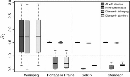
Sensitivity of the general ${\mathcal{R}}_0$ to variations of ${\mathcal{R}}_0^x$ between 0.5 and 3, where $x$ is the city indicated on the $x$ axis. The box shows the extent of results between the 25th and 75th percentile, while the whiskers extend to the most extreme values. The bar in the box is the median. The sensitivity to changes in ${\mathcal{R}}_0^W$ when the disease is in Winnipeg is irrelevant and is not represented

In Fig. 2, it can be seen that, with the parameters used, most of the variation of ${\mathcal{R}}_0$ is driven by Winnipeg; the small cities have little influence, albeit varying: Portage la Prairie can trigger a bifurcation even when ${\mathcal{R}}_0^W<1$, while Steinbach has a more limited influence and variations of ${\mathcal{R}}_0^2$ in Selkirk have almost no effect on the value of the general ${\mathcal{R}}_0$.

Influence of connectivity

Understanding the roles of the satellite cities requires to consider not only their size, but the rates of movement that connect them to Winnipeg. From Table 1, daily travellers to and from Winnipeg represent approximately 32, 81 and 55 % of the respective populations of Portage la Prairie, Selkirk and Steinbach and these percentages are reflected in the actual movement rates.

High connectivity implies indistinguishibility

As remarked in Fig. 2, variations of ${\mathcal{R}}_0^2$ in Selkirk have almost no impact on variations of the general ${\mathcal{R}}_0$, regardless of the scenario considered for ${\mathcal{R}}_0^x$ in the other cities. Selkirk is the closest satellite to Winnipeg and has the highest ratio of trips to inhabitants and thus, the highest movement rates. The average time an individual spends in Selkirk (their residence time there) is small. In a sense, this community is barely distinguishable from Winnipeg and additional sensitivity analysis (not shown) indicates that it does not really matter whether one considers it as part of Winnipeg or separated.

Lower connectivity can drive ${\mathcal{R}}_0$

Portage la Prairie and Steinbach have comparable populations. However, with the parameters under consideration and with reasonable values of the ${\mathcal{R}}_0^x$, it can be seen in Fig. 2 that only the former can cause the general ${\mathcal{R}}_0$ to take values larger than 1 when ${\mathcal{R}}_0^W<1$. Intuition indicates that this must be due to the movement rate. If all movement rates were zero, then ${\mathcal{R}}_0$ would be given by

$$\begin{array}{c}\hfill {\mathcal{R}}_0=max\{{\mathcal{R}}_0^W,{\mathcal{R}}_0^1,{\mathcal{R}}_0^2,{\mathcal{R}}_0^3\},\end{array}$$

since the matrix $F{V}^{-1}$ is diagonal when $\mathcal{M}=0$. As movement rates to and from Portage la Prairie are lower, the situation is closer to the uncoupled case and the value of ${\mathcal{R}}_0^1$ has more impact on the general ${\mathcal{R}}_0$.

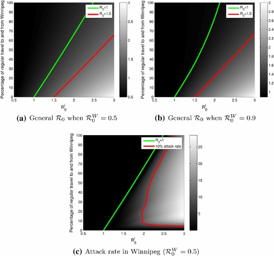
This is confirmed by Fig. 3a, which shows the joint effect of a reduction of movement between Winnipeg and Portage la Prairie and of the value of ${\mathcal{R}}_0^1$ in Portage la Prairie, when ${\mathcal{R}}_0^W={\mathcal{R}}_0^{2,3}=0.5$. On this figure, ${\mathcal{R}}_0<1$ is located above the green curve. When Portage la Prairie is completely isolated from Winnipeg (bottom of the figure), the value of ${\mathcal{R}}_0^1$ governs the value of the general ${\mathcal{R}}_0$. This effect decreases as the movement rates increase.

Fig. 3.

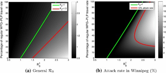
Plots as functions of ${\mathcal{R}}_0^1$ in Portage la Prairie and the reduction of movement between Winnipeg and Portage la Prairie. a General ${\mathcal{R}}_0$; the green and red curves show the locations of ${\mathcal{R}}_0=1$ and ${\mathcal{R}}_0=1.5$, respectively. b Attack rate in Winnipeg; the green and red curves show the locations of ${\mathcal{R}}_0=1$ and a 10 % attack rate, respectively

Lower connectivity has little effect on severity

Although Portage la Prairie can drive the value of the general ${\mathcal{R}}_0$, its effect on other aspects of disease dynamics is not as important as that of Winnipeg. Figure 3b shows the attack rate in Winnipeg as a function of the same parameters as those in Fig. 3a. Attack rates are a fundamental concept in epidemiology that are used to quantify the burden of an epidemic over its time course. The term “rate” is a misnomer, as most of the time, attack rates refer to the percentage of individuals in a population that have borne the pathogen during the epidemic; however, this is the most commonly used term to describe this concept and it is therefore used here.

In order to obtain attack rates as in Fig. 3b, the following approximation method is used. Numerical solutions to the ODE are computed over a time period. The number of infection-days for a given community $x$ is then obtained by trapezoidal integration of $I_x(t)$. This is converted in turn to a number of infections by dividing by the average duration of the infectious period (4.1 days). Finally, this is related to the population $N_x^{\ast }$ and converted to percentage. In order to obtain comparable results, all attack rates graphs are produced here using simulations for 1 year.

Considering Fig. 3b, one sees that in most cases, even in situations where ${\mathcal{R}}_0^1$ causes the whole system to go to an endemic equilibrium (below the green curve), the attack rate remains low in Winnipeg. To obtain attack rates over 10 % in a “normal” movement context, ${\mathcal{R}}_0^1$ must be quite high, well over 2 (red curve). To put things in perspective, most influenza epidemics, whether annual or pandemic, have estimated ${\mathcal{R}}_0$ values around 1.5. Pandemic planning scenarios prior to the 2009 H1N1 pandemic made assumptions placing the attack rate between 15 and 35 % for mild and severe scenarii, respectively; see Sect. Two in Public Health Agency of Canada (2006). Interestingly, the higher values of ${\mathcal{R}}_0$ are obtained in regions of parameter space where the attack rate in Winnipeg is small (lower right corner).

Connectivity acts differently on ${\mathcal{R}}_0$ and the attack rate

Figure 3a, b also illustrate another interesting property of the system: while ${\mathcal{R}}_0$ appears to depend linearly on ${\mathcal{R}}_0^1,m_{1W}$ and $m_{W1}$ (green curve in both figures), the attack rate is more complex (red curve in Fig. 3b). Suppose for instance that ${\mathcal{R}}_0^1$ were a little larger than 2.5, placing the system in a region where ${\mathcal{R}}_0>1$ but with an attack rate less than 10 % in Winnipeg. Then reducing the rate of movement between Winnipeg and Portage la Prairie to 50 % of its usual value would result in a marked increase of the attack rate. It is only by bringing movement to less than 10 % of its default value that the attack rate in Winnipeg would be made smaller.

The urban centre drives ${\mathcal{R}}_0$ and disease severity

Continuing on the relative roles of the urban centre, Winnipeg, and its least connected satellite, Portage la Prairie, it can be seen in Fig. 4 that the effect of raising the value of ${\mathcal{R}}_0^1$ is much less than the effect of raising the value of ${\mathcal{R}}_0^W$, both in terms of effect on the general ${\mathcal{R}}_0$ (Fig. 4a) or in terms of the overall attack rate (Fig. 4b). If only one of ${\mathcal{R}}_0^W$ or ${\mathcal{R}}_0^1$ is allowed to vary (moving horizontally or vertically in the figure), then a reduction of the attack rate from 30 to 5 % requires little change to ${\mathcal{R}}_0^W$ (provided ${\mathcal{R}}_0^1$ is not too large), whereas a lot more reduction of ${\mathcal{R}}_0^1$ is needed to achieve the same effect. Similarly, reducing the value of the general ${\mathcal{R}}_0$ to a value less than 1 is only achievable by acting on ${\mathcal{R}}_0^1$ if ${\mathcal{R}}_0^W$ is already less than 1.

Fig. 4.

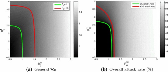
Plots as functions of ${\mathcal{R}}_0^W$ (Winnipeg) and ${\mathcal{R}}_0^1$ (Portage la Prairie). a Value of the general ${\mathcal{R}}_0$; the green and red curves show the location of ${\mathcal{R}}_0=1$ and $1.5$, respectively. b Overall attack rate; the green and red curves are 5 and 30 %, respectively

Note that the situation is similar if ${\mathcal{R}}_0^i,i=1,2,3$, is made to vary instead of just ${\mathcal{R}}_0^1$ (not shown).

Curtailing an epidemic

The question of “control” is now considered. In this model, there are two separate mechanisms that can be used to control the epidemic: the value of ${\mathcal{R}}_0^x$ can be lowered or mobility can be restrained. In order to evaluate the relative value of such measures, the following experiments are conducted.

Protection of satellite cities from disease in Winnipeg

In Fig. 5, ${\mathcal{R}}_0^i=0.5,i=1,2,3,{\mathcal{R}}_0^W\in [0.5,3]$ and the rate of movement to and from Winnipeg varies from 0 to 100 % of its standard value. Changing the value of ${\mathcal{R}}_0^i$ to, say, 0.9 (not shown), does not change the situation: the effect of a reduction of the movement rate is almost null, control of the general ${\mathcal{R}}_0$ is only achievable through control of ${\mathcal{R}}_0^W$, as can be seen in Fig. 5a. On the other hand, as shown in Fig. 5b, reducing the rate of movement between Winnipeg and the satellite cities to a very low value can help lower the disease attack rate in the satellite cities when ${\mathcal{R}}_0^W$ is large.

Fig. 5.

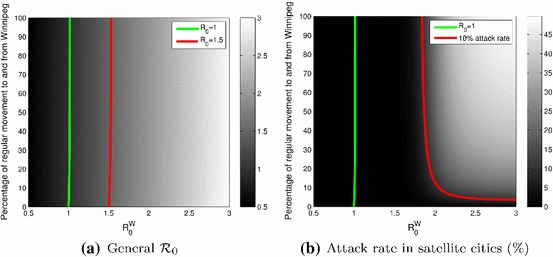
General ${\mathcal{R}}_0$ (a) and attack rate in the satellite cities (b) as a function of ${\mathcal{R}}_0^W$ in Winnipeg and the reduction in movement rate between Winnipeg and the satellite cities. The satellite cities have ${\mathcal{R}}_0^i=0.5,i=1,2,3$

Protection of Winnipeg from disease in satellite cities

In Fig. 6, ${\mathcal{R}}_0^i\in [0.5,3],i=1,2,3$ and the rate of movement to and from Winnipeg varies from 0 to 100 % of its standard value. Comparing Fig. 6a, where ${\mathcal{R}}_0^W=0.5$ and Fig. 6b, where ${\mathcal{R}}_0^W=0.9$, one sees that when the reproduction number in Winnipeg is larger, the amount of effort required to bring the general ${\mathcal{R}}_0$ to a value less than 1 increases, as the value of ${\mathcal{R}}_0^i$ at which ${\mathcal{R}}_0=1$ is smaller in Fig. 6b.

Fig. 6.

Plots as functions of ${\mathcal{R}}_0^i,i=1,2,3$ taken equal and the percentage of the regular movement rates between Winnipeg and the satellite cities. a Case where ${\mathcal{R}}_0^W=0.5$. b Case where ${\mathcal{R}}_0^W=0.9$. c Attack rate in Winnipeg, in %, when ${\mathcal{R}}_0^W=0.5$

Here again, as in the case with only Portage la Prairie and Winnipeg, decreasing the movement rates results in an increase of ${\mathcal{R}}_0$. However, as seen in Fig. 6c, a decrease of the rates of movement has a much more complicated effect on the attack rate in Winnipeg. While a moderate decrease would be detrimental to the attack rate, a radical decrease of movement rates would lower the attack rate.

Discussion

An SIR metapopulation model for the spread of an infectious disease between a large urban centre and smaller neighbouring satellite cities was considered. Because of the widely different population sizes, different incidence functions were used in the urban centre (standard incidence) and the satellite cities (mass action incidence).

Note that in the present work, death and recovery rates were taken equal in all locations. This is appropriate for the application to Winnipeg and neighbouring satellite cities. However, several communities in Northern Manitoba are in a configuration that closely resembles that of satellite communities: they are accessible only by air or (during the winter) using ice roads. Per capita air travel rates from these communities to and from Winnipeg is much higher than the average travel rate between larger sized Canadian cities. For instance, using the method of computation of travel rates explained earlier and air transportation data from the BioDiaspora Project (see, e.g., Arino and Khan 2014), it is found that, in 2012, the per capita rate of air travel from Churchill (Manitoba) to Winnipeg was almost 450 times that from Toronto to Winnipeg and still more than 50 times the total rate out of Toronto to all 1,600 final destinations reached from there in 2012. Statistics Canada data (http://www.statcan.gc.ca/health-sante/index-eng.htm) shows that in 2013, for the Burntwood/Churchill Health Region that comprises all of Northern Manitoba, the average life expectancy at birth was 71.0 years (compared to Canada’s 81.1 years or Winnipeg’s 80.1 years). Several of these communities have no resident doctor. In this context, the rates of recovery and death could be assumed to differ.

The first objective of this work was to study mathematically the effect of coupling together cities with different functional forms for incidence. The total population in each patch was shown to converge to a positive value. An expression for the general basic reproduction number ${\mathcal{R}}_0$ was derived. The global asymptotic stability of the unique disease free equilibrium when ${\mathcal{R}}_0\le 1$ was established. The proof followed that in the paper of Li and Shuai (2009). Interestingly, the Lyapunov function used by Li and Shuai (2009) for a system with all incidence functions of the same type can be adapted easily to the present heterogeneous case. The uniform persistence of the system as well as the existence of an endemic equilibrium were shown by setting other results by Li and Shuai (2009) in an asymptotically autonomous setting. It is suspected that when ${\mathcal{R}}_0>1$, there is a unique globally asymptotically stable endemic equilibrium. However, here the method of proof used by Li and Shuai (2009) was not applicable because of restrictions on the movement matrices there and more work will be needed to prove this. It was finally shown that under some conditions, the general ${\mathcal{R}}_0$ is bounded below and above by the minimum and maximum values of the individual ${\mathcal{R}}_0^x$ in the cities.

The second objective of this work was to investigate a real life situation. For this, Winnipeg and its three main satellite cities were used with parameters appropriate for influenza. One possible mechanism for deriving rates of movement between cities was discussed, using estimates of the average daily number of car trips between Winnipeg and the three smaller cities that were obtained in Appendix . It was observed that the large city, Winnipeg, governed for the most part the behaviour of the system. Only Portage la Prairie, which has the smallest rate of movement to and from Winnipeg, was able to trigger an epidemic if all other cities (including Winnipeg) had a low value of ${\mathcal{R}}_0^x=0.5$. It was observed that, as far as the satellite cities are concerned, reducing the value of ${\mathcal{R}}_0^W$ was much more important than isolating from Winnipeg, since only almost perfect isolation was able to curb the overall attack rate of the disease in the case that ${\mathcal{R}}_0^W>1$.

These numerical results provide a glimpse into the dynamics of infectious diseases in a satellite-central hub setting and highlight the major role played by the main urban centre on the course of an epidemic in such a system. They also emphasize the fact that not all satellite cities play equal roles, with the three cities considered here having different capacities to influence the dynamics of infection in the overall system, depending on the nature of their connection to the main urban centre.

Note that when it holds, the bounds given by Proposition 3 allow, for system (1), to answer in the negative an often difficult question in metapopulation models: can movement “make it worse”, in the sense that the general ${\mathcal{R}}_0$ would take values larger than any the individual ${\mathcal{R}}_0^x$? Numerical simulations were conducted in a context where this proposition does hold, highlighting one issue with numerics: because the total population is asymptotically constant in each patch and that simulations are conducted at that equilibrium, the effect of having different functional forms for incidence is very small. Numerical simulations (not shown) were conducted which show that, with the parameters used, one obtains virtually the same plots as in Fig. 4 if mass action or proportional incidence are used in all cities.

Finally, note that Figs. 3,  5 and 6 tell a cautionary tale: ${\mathcal{R}}_0$ is, in the context of mathematical models such as the one here, a bifurcation parameter that allows to distinguish between two dynamical regimes. However, ${\mathcal{R}}_0$ does not give the whole story. Take for instance Fig. 3 and suppose ${\mathcal{R}}_0^1=2.5$ and the movement rate is at 30 % of standard, i.e., a point slightly below the red curve in Fig. 3a. Suppose that the only control measure available is to act on the movement rates. If one only considers Fig. 3a, then the obvious solution is to encourage more travel. However, Fig. 3b suggests that decreasing the movement rate further would be a much better strategy.

In view of the remarks above, it is clear that the ordinary differential equations framework used here is somewhat limiting and that further work should consider a stochastic approach such as the one used by Arino et al. (2011); Arino and Khan (2014) or Lindholm and Britton (2007). The latter considers a different framework, with an implicit description of movement, but shows that a derivation of some important quantities such as the mean time to extinction of the infection is probably possible in the stochastic equivalent of the model considered here.

Appendix: Estimating daily trips

Contrary to data on air (Arino and Khan 2014) or train transportation, UMTIG transportation data is not usable directly in the model as it provides flows through points, not trips between locations. Among the vehicles counted at a given counting station, it is not possible to distinguish the ones making a trip between the cities of concern from the ones making either a longer or a shorter trip. Therefore, the numbers obtained here are an approximation.

Observe that the volume of movement on a given route between two locations can be no larger than the minimum of the values obtained at the counting stations on that route between the two locations. So the volume obtained is a loose upper bound. Canadian Vehicle Survey data for 2009 shows that the average vehicle occupancy in Manitoba was 1.65 persons per light vehicle; see Fig. 12 in the report by the Office of Energy Efficiency (2009). Numbers could be further adjusted to take into account this fact. However, due to the already present uncertainty, the raw estimated number of vehicles is used. Lastly, it is assumed that individuals usually try to optimize the length of their trips (whether in distance or in time) and thus avoid complicated alternate routes. Therefore, only the most direct routes between locations are considered.

Only the estimation of the volume between Winnipeg and Portage la Prairie is shown here. The other two proceed similarly. In practice, the traffic inbound from Winnipeg is captured by stations 368 and 2077 (see Fig. 7). The last available date for station 368 is 1993. In order to get a more recent estimate, note that traffic through stations 48 and 369 increased an average 31.5 % in the eastbound direction and 37.5 % in the westbound direction, from 1993 to 2011. Adjusting the 1993 estimates for station 368 similarly gives 3,840 vehicles eastbound and 4,015 westbound. Station 2077 has a 2011 estimate of 5,430 vehicles. This is the total of northbound and southbound traffic. Because no further information is available, assume that traffic is split evenly between northbound and southbound vehicles, thus there are 2,715 vehicles travelling in each direction daily. Consider northbound vehicles. They may come from Highway 1 from both directions, or from further south on Highway 240. The latter are captured by station 366, which shows an undirected daily average traffic of 4,680 vehicles, i.e., 2,340 in each direction. Thus, the daily northbound flux of “nonresidents” is estimated to be 375 vehicles. Again, this is split evenly between traffic incoming from Highway 1 westbound and eastbound, giving a total of 188 vehicles coming from Winnipeg. The same volume is estimated to go to Winnipeg each day. Adding the volumes gives a total number of travellers to Winnipeg of 4,028, while there are 4,203 travellers from Winnipeg. To simplify a little further given the already present uncertainty, the average (rounded below) of these two values is used in both directions, giving the number in Table 1.

Fig. 7.

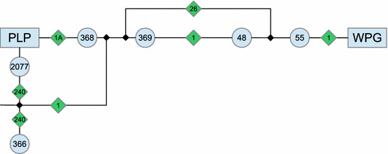
Schematization of the location of the vehicle counters used to estimate traffic between Winnipeg (WPG) and Portage la Prairie (PLP). The numbers in disks refer to UMTIG counting stations, those in diamonds are road numbers

References

- Arino J (2009) Diseases in metapopulations. In: Ma Z, Zhou Y, Wu J (eds) Modeling and dynamics of infectious diseases. World Scientific Publishing, Singapore, pp 65–123
- Arino J, Khan K. Using mathematical modelling to integrate disease surveillance and global air transportation data. In: Chen D, Moulin B, Wu J, editors. Analyzing and modeling spatial and temporal dynamics of infectious diseases. New York: Wiley; 2014. pp. 97–108. [Google Scholar]
- Arino J, McCluskey CC. Effect of a sharp change of the incidence function on the dynamics of a simple disease. J Biol Dyn. 2010;4(5):490–505. doi: 10.1080/17513751003793017. [DOI] [PubMed] [Google Scholar]
- Arino J, Brauer F, van den Driessche P, Watmough J, Wu J. Simple models for containment of a pandemic. J Royal Soc Interface. 2006;3(8):453–457. doi: 10.1098/rsif.2006.0112. [DOI] [PMC free article] [PubMed] [Google Scholar]
- Arino J, Hu W, Khan K, Kossowsky D, Sanz L. Some methodological aspects involved in the study by the Bio. Diaspora Project of the spread of infectious diseases along the global air transportation network. Can Appl Math Quart. 2011;19(2):125–137. [Google Scholar]
- Berman A, Plemmons RJ. Nonnegative matrices in the mathematical sciences. New York: SIAM; 1994. [Google Scholar]
- Berman A, Shaked-Monderer N (2012) Non-negative matrices and digraphs. Comput Complex 2082–2095. doi:10.1007/978-1-4614-1800-9_132
- Fromont E, Pontier D, Langlais M. Disease propagation in connected host populations with density-dependent dynamics: the case of the Feline Leukemia Virus. J Theor Biol. 2003;223:465–475. doi: 10.1016/S0022-5193(03)00122-X. [DOI] [PubMed] [Google Scholar]
- Horn R, Johnson C. Matrix analysis. 2. Cambridge: Cambridge University Press; 2013. [Google Scholar]
- Khan K, Arino J, Hu W, Raposo P, Sears J, Calderon F, Heidebrecht C, Macdonald M, Liauw J, Chan A, Gardam M (2009) Spread of a novel influenza A (H1N1) virus via global airline transportation. N Engl J Med 361(2):212–214 [DOI] [PubMed]
- Korobeinikov A, Wake GC. Lyapunov functions and global stability for SIR, SIRS, and SIS epidemiological models. Appl Math Lett. 2002;15:955–960. doi: 10.1016/S0893-9659(02)00069-1. [DOI] [Google Scholar]
- Li MY, Shuai Z. Global stability of an epidemic model in a patchy environment. CAMQ. 2009;17(1):175–187. [Google Scholar]
- Lindholm M, Britton T. Endemic persistence or disease extinction: the effect of separation into sub-communities. Theor Popul Biol. 2007;72:253–263. doi: 10.1016/j.tpb.2007.05.001. [DOI] [PubMed] [Google Scholar]
- McCallum H, Barlow N, Hone J. How should pathogen transmission be modelled? Trends Ecol Evol. 2001;16(6):295–300. doi: 10.1016/S0169-5347(01)02144-9. [DOI] [PubMed] [Google Scholar]
- Office of Energy Efficiency (2009) Natural resources Canada Canadian vehicle survey. Tech Rep M141–18/2009E-PDF
- Public Health Agency of Canada (2006) The Canadian Pandemic Influenza Plan for the Health Sector. http://www.phac-aspc.gc.ca/cpip-pclcpi/index-eng.php. Accessed 24 September 2014
- Thieme HR. Uniform persistence and permanence for non-autonomous semiflows in population biology. Math Biosci. 2000;166(2):173–201. doi: 10.1016/S0025-5564(00)00018-3. [DOI] [PubMed] [Google Scholar]
- van den Driessche P, Watmough J. Reproduction numbers and sub-threshold endemic equilibria for compartmental models of disease transmission. Math Biosci. 2002;180:29–48. doi: 10.1016/S0025-5564(02)00108-6. [DOI] [PubMed] [Google Scholar]
- Vargas-De-León C. On the global stability of SIS, SIR and SIRS epidemic models with standard incidence. Chaos Solitons Fractals. 2011;44:1106–1110. doi: 10.1016/j.chaos.2011.09.002. [DOI] [Google Scholar]
- Wang W, Zhao X-Q. Threshold dynamics for compartmental epidemic models in periodic environments. J Dyn Diff Equ. 2008;20(3):699–717. doi: 10.1007/s10884-008-9111-8. [DOI] [Google Scholar]