Modeling Tumor Growth and Treatment Resistance Dynamics Characterizes Different Response to Gefitinib or Chemotherapy in Non‐Small Cell Lung Cancer

Abstract

Differences in the effect of gefitinib and chemotherapy on tumor burden in non‐small cell lung cancer remain to be fully understood. Using a Bayesian hierarchical model of tumor size dynamics, we estimated the rates of tumor growth and treatment resistance for patients in the Iressa Pan‐Asia Study study (NCT00322452). The following relationships characterize greater efficacy of gefitinib in epidermal growth factor receptor (EGFR) positive tumors: Maximum drug effect is, in decreasing order, gefitinib in EGFR‐positive, chemotherapy in EGFR‐positive, chemotherapy in EGFR‐negative, and gefitinib in EGFR‐negative tumors; the rate of resistance emergence is, in increasing order: gefitinib in EGFR positive, chemotherapy in EGFR positive, while each is plausibly similar to the rate in EGFR negative tumors, which are estimated with less certainty. The rate of growth is smaller in EGFR‐positive than in EGFR‐negative fully resistant tumors, regardless of treatment. The model can be used to compare treatment effects and resistance dynamics among different drugs.

Study Highlights.

• WHAT IS THE CURRENT KNOWLEDGE ON THE TOPIC?

☑ Differences in tumor response between drugs have been described with models of tumor size dynamics, ranging from empirical to highly mechanistic models. Complex mechanistic models provide limited insight into fundamental features of tumor response such as initial drug‐induced tumor regression and its eventual regrowth, given the sparse measurements of the total size of tumor lesions. Empirical models match their complexity to the amount of data but are less interpretable.

• WHAT QUESTION DID THIS STUDY ADDRESS?

☑ What are the differences in key features of tumor growth dynamics underlying differences in response to treatment between drugs?

• WHAT DOES THIS STUDY ADD TO OUR KNOWLEDGE?

☑ We used a Bayesian hierarchical population dynamics model of tumor size to compare tumor response between chemotherapy and gefitinib (targeting epidermal growth factor receptor (EGFR)) for non‐small cell lung cancer. The parameters of the model have clear interpretation: The rate of tumor growth, the maximum drug effect on the growth rate, and the rate of emerging resistance. Estimated distributions of parameters values given clinical tumor size data showed that superior efficacy of gefitinib in EGFR‐mutated tumors is explained by a larger initial drug effect on tumor size reduction and a slower rate of resistance emergence compared with chemotherapy and to gefitinib in EGFR‐negative tumors.

• HOW MIGHT THIS CHANGE DRUG DISCOVERY, DEVELOPMENT, AND/OR THERAPEUTICS?

☑ The model can be used to estimate drug effects and their resistance dynamics from small trials by regularizing the estimates from small data sets against “prior” distributions of parameters inherent in a Bayesian model of historical tumor response data. The structure of the model and clearly interpretable parameters are versatile to describe a typical pattern of tumor response (initial size decrease followed by eventual regrowth) will facilitate the comparison of drug effects and resistance dynamics among drugs with the mechanism of action and the use of the tumor dynamics model in the joint modeling of tumor response and survival events.

Lung cancer is one of the most common cancers comprising 11.6% of all new cancer cases in the United States in 2016, with a low 5‐year relative survival rate of 20.6% in patients diagnosed in 2009–2015.1 Non‐small cell lung cancer (NSCLC) comprises most lung cancers and now has multiple therapeutic options, including chemotherapy, molecularly targeted agents, and immune therapy.2 Gefitinib is one such targeted agent that inhibits the kinase activity of the epidermal growth factor receptor (EGFR). It was approved in 2003 by the U.S. Food and Drug Administration for treatment of patients with locally advanced or metastatic NSCLC. EGFR is a transmembrane receptor activated by the epidermal growth factor that promotes cell proliferation. NSCLC patients who have specific activating mutations in the kinase domain of the EGFR gene are responsive to gefitinib.3 Many studies have compared effectiveness of chemotherapy and gefitinib monotherapy or in combination with chemotherapy.4 The relationship between differences in the effect of gefitinib and chemotherapy on tumor burden and differences in the effect on survival remains to be fully understood.

Tumor burden, measured by the sum of longest diameters (SLD) of tumor lesions (linear tumor size) is a key component of the Response Evaluation Criteria in Solid Tumors (RECIST).5 The rate and extent of change in tumor size is a measure of effectiveness of therapy. The modeling of dynamics of tumor size in response to treatment is key to understanding how the rate and extent of tumor progression depends on patient characteristics and therapy. Tumor dynamics models play a key role in the joint modeling of longitudinal tumor size and progression and survival events.6 This has the potential to use predicted survival with the joint models7 for individual treatment decisions at the point of care and as an end point in clinical trials. An early application of this idea used a survival model with the change of tumor size from baseline at the first visit as a covariate to predict survival in a phase III trial of capecitabine in metastatic colorectal cancer using the change of tumor size estimated in a phase II trial.8

A plethora of tumor dynamic models has been proposed.9 One class of models is population dynamics models. They describe tumor size change in response to drug treatment using a differential equation for the number of tumor cells, in which the net rate is a sum of positive (cell “birth”) and negative (cell “death”) terms. Trivially, these terms are linear in tumor size (a linear model) describing the exponential growth when the net rate is constant and positive. Other models use more complex terms leading to, e.g., Gompertz growth. A seminal model10 describing the Gompertz growth of tumors can be understood as a linear model where the net positive rate decreases exponentially over time. A more recent linear model8 applied the exponential “retardation” effect to the “death” rate, such that the net rate of tumor size change could change sign from negative (net decrease upon initiation of therapy) to positive (net increase during emerging resistance to therapy).

In this article, we used the model of Claret et al.8 to estimate and compare the parameters describing the extent of drug effect, rate of resistance emergence, and growth rate of a fully resistant tumor in patients who are wild‐type or positive for EGFR‐activating mutations treated with gefitinib or chemotherapy in the Iressa Pan‐Asia Study (IPASS) study (NCT00322452).11

Methods

Clinical data

The IPASS study (NCT00322452) was a phase III, multicenter, randomized, open‐label, parallel‐group study comparing gefitinib (Iressa, AstraZeneca, Macclesfield, UK) with carboplatin (Paraplatin, Bristol‐Myers Squibb, New York, NY) plus paclitaxel (Taxol, Bristol‐Myers Squibb) as first‐line treatment in clinically selected patients in East Asia who had advanced NSCLC. The primary end point was progression‐free survival. Secondary end points included overall survival, the objective response rate, quality of life, reduction in symptoms, safety, and the adverse‐event profile.11

The analysis set for modeling, extracted from the IPASS study, comprised 1,837 tumor measurements from 344 NSCLC patients aged from 27 to 82 (first quartile 51, median 59, third quartile 67). One third (124) of the patients were of Chinese descent, followed by Japanese (91), Asian other than Chinese and Japanese (128), and other (1). Patients were randomly assigned two treatment arms, gefitinib or chemotherapy (carboplatin/paclitaxel). Both EGFR‐positive patients based on biopsy (n = 219) and EGFR‐negative patients  (n = 125) were randomized into both treatment arms. The numbers of patients assigned to gefitinib were 111 and 59 in the EGFR‐positive groups and EGFR‐negative groups, respectively. The chemotherapy arm had 108 and 66 in the EGFR‐positive groups and EGFR‐negative groups, respectively. Each patient’s longitudinal tumor burden was measured by imaging 5.34 times on average (maximum 17), with imaging follow‐up lasting 25.94 weeks on average (maximum 96.86 weeks). Tumor load measurements followed the RECIST criteria,5 with identification and longitudinal tracking of the SLD of up to five target lesions. We used SLD to characterize tumor size for modeling because it is the standard measure of tumor load in clinical trials.5

All patients provided written informed consent; separate consent was provided for the assessment of the EGFR biomarkers. An independent ethics committee at each participating institution approved the study protocol. The study was conducted in accordance with the Declaration of Helsinki, the International Conference on Harmonization Guidelines for Good Clinical Practice, applicable regulatory requirements, and AstraZeneca's policy on bioethics.

A tumor dynamics model

Let $y\left(t\right)$ be tumor volume at time $t$, approximated by a sphere with the diameter equal to SLD, $\frac{4}{3}\pi {\left(\frac{\text{SLD}}{2}\right)}^3$ (volumetric tumor size). This volume is proportional to the total number of tumor cells supporting use of a population dynamics model to describe $y\left(t\right)$, as can be seen from the following considerations. In the case of two lesions, $\text{SLD}=D_1+D_2$ is the sum of diameters of the two lesions. The cube of the sum expands into where $V_1$ and $V_2$ are spherical volumes.

$$\begin{array}{cc}\hfill \frac{\pi }{6}{\text{SLD}}^3& =\frac{\pi }{6}\left(D_1^3+3D_1^2{D}_2+3D_2^2{D}_1+D_2^3\right)\hfill \\ & =\frac{\pi }{6}\left(\frac{6}{\pi }{V}_1+3{\left(\frac{6}{\pi }{V}_1\right)}^{2/3}{\left(\frac{6}{\pi }{V}_2\right)}^{1/3}+3{\left(\frac{6}{\pi }{V}_2\right)}^{2/3}{\left(\frac{6}{\pi }{V}_1\right)}^{1/3}+\frac{6}{\pi }{V}_2\right)\hfill \\ & =V_1+3V_1^{2/3}{V}_2^{1/3}+3V_2^{2/3}{V}_1^{1/3}+V_2\hfill \end{array}$$

Considering that the mean volume of tumor cell, $V_{\text{cell}}$, is similar among the lesions from

$$V_1=N_1{V}_{\text{cell}},V_2=N_2{V}_{\text{cell}}$$

we obtain the following:

$$\frac{\pi }{6}{\text{SLD}}^3=V_{\text{cell}}\left(N_1+3N_1^{2/3}{N}_2^{1/3}+3N_2^{2/3}{N}_1^{1/3}+N_2\right).$$

Considering that the number of cells in the lesions are not very different from each other, the expression is approximately proportional to the sum of tumor cells in both lesions. An illustrative example supporting the approximate linear relationship is provided in the Supplemental Information (Figure S1 and Table S1). The argument is the same for more than two lesions.

Because tumor volume is approximately proportional to the total number of tumor cells, it is described by the following differential equation using population dynamics considerations and considering cells in all lesions have similar dynamic rates:

$$\frac{\mathrm{d}y\left(t\right)}{\mathrm{d}t}=\mathrm{\lambda }y\left(t\right)-\mathrm{\mu }y\left(t\right)=\left(\mathrm{\lambda }-\mathrm{\mu }\right)y\left(t\right),$$ (1)

where $\mathrm{\lambda }$ is the rate of tumor cell “birth,” and $\mathrm{\mu }$ is rate of tumor cell “death.” Tumor volume increases exponentially when the net rate $\left(\mathrm{\lambda }-\mathrm{\mu }\right)$ is positive and decreases exponentially when it is negative.

Note that Eq. 1 can be used to model either SLD or SLD³. This is because this model, as well as the logistic and Gompertz models, are invariant under power transformation of SLD and exhibit the same dynamics of tumor size whether it is measured as SLD or SLD³. We chose to fit our model to tumor volume to lay the foundation for developing it into more complex, nonlinear models. For nonlinear population models, the dynamics of the number of cells is different than the dynamics of the linear scale (SLD) because they change form when transforming from volume to SLD.

To describe the typical tumor volume pattern of initial decrease upon initiation of treatment followed by eventual increase, the net rate must start out negative then change its sign to positive. Without loss of generality, we assume that at the start of treatment the “birth” rate $\mathrm{\lambda }\left(t\right)$ is inhibited by gefitinib or chemotherapy to a low value, ${\mathrm{\lambda }}_{min}$, then increases exponentially to ${\mathrm{\lambda }}_0$ over time, representing the rise of resistance to treatment:

$$\mathrm{\lambda }\left(t\right)={\mathrm{\lambda }}_0-\left({\mathrm{\lambda }}_0-{\mathrm{\lambda }}_{min}\right)e^{-\mathrm{\alpha }t},$$

where $\mathrm{\alpha }$ determines the rate of resistance emergence. A drug with smaller $\mathrm{\alpha }$ will maintain inhibitory effect for longer than a drug with larger $\mathrm{\alpha }$. Defining $k_{\text{gr}}:={\mathrm{\lambda }}_0-\mathrm{\mu }$ and ${\mathrm{\Delta }}_{\mathrm{\lambda }}:={\mathrm{\lambda }}_0-{\mathrm{\lambda }}_{min}$, we obtain the following tumor dynamic model, which has the same form as in Claret et al.8:

$$\begin{array}{cc}\frac{dy\left(t\right)}{\mathit{dt}}\hfill & =\left[{\mathrm{\lambda }}_0-\left({\mathrm{\lambda }}_0-{\mathrm{\lambda }}_{min}\right)e^{-\mathrm{\alpha }t}-\mathrm{\mu }\right]y\left(t\right)\hfill \\ \hfill & =\left[({\mathrm{\lambda }}_0-\mathrm{\mu })-\left({\mathrm{\lambda }}_0-{\mathrm{\lambda }}_{min}\right)e^{-\mathrm{\alpha }t}\right]y\left(t\right)\hfill \\ \hfill & :=k_{\text{gr}}y\left(t\right)-{\mathrm{\Delta }}_{\mathrm{\lambda }}{e}^{-\mathrm{\alpha }t}y\left(t\right).\hfill \end{array}$$

Note that $k_{\text{gr}}$ describes the net tumor growth rate after the drug inhibitory effect has worn off (fully resistant tumor that grows despite continuing drug treatment) and ${\mathrm{\Delta }}_{\mathrm{\lambda }}$ describes the maximum intensity of the drug effect on the “birth” rate at the start of treatment when no resistance is present. As time goes from 0 to $\infty$, the net growth rate of the tumor changes from $k_{\text{gr}}-{\mathrm{\Delta }}_{\mathrm{\lambda }}$ (negative, decreasing tumor volume) to $k_{\text{gr}}$ (positive, increasing tumor volume). The relations among parameters and a typical time profile of tumor volume are schematically described in Figure 1. The solution of the ordinary differential equation is:

$$y\left(t\right)=K_0\exp \left(k_{\text{gr}}t+\frac{{\mathrm{\Delta }}_{\mathrm{\lambda }}}{\mathrm{\alpha }}{e}^{-\mathrm{\alpha }t}\right),$$

where $K_0$ is an initial value which satisfies $y\left(0\right)=K_0\exp \left(\frac{{\mathrm{\Delta }}_{\mathrm{\lambda }}}{\mathrm{\alpha }}\right):=y_0$. Then one can reparameterize the model using $y_0$ as follows:

$$\begin{array}{cc}y\left(t\right)\hfill & =y_0\exp \left(-\frac{{\mathrm{\Delta }}_{\mathrm{\lambda }}}{\mathrm{\alpha }}\right)\exp \left(k_{\text{gr}}t+\frac{{\mathrm{\Delta }}_{\mathrm{\lambda }}}{\mathrm{\alpha }}{e}^{-\mathrm{\alpha }t}\right)\hfill \\ \hfill & =y_0\exp \left(k_{\text{gr}}t-\frac{{\mathrm{\Delta }}_{\mathrm{\lambda }}}{\mathrm{\alpha }}\left(1-e^{-\mathrm{\alpha }t}\right)\right)\hfill \end{array}$$ (2)

Figure 1.

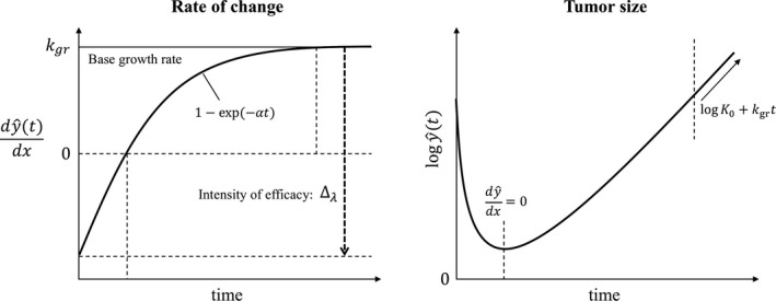
Schematic of the tumor dynamic model. y is tumor volume at time t.

Let $m$ be observed tumor volume and assume observations are independently, identically, log‐normally distributed, the measurement model is expressed as:

$$m\sim \log \mathcal{N}(\log y\left(t\right),\mathrm{\sigma }),$$

where $\mathrm{\sigma }$ is standard deviation of the measurement error.

A hierarchical Bayesian model

Tumor dynamics profiles on treatment vary greatly among patients. In a hierarchical model, individual patient parameters $y_{0,i},k_{\text{gr},i},{\mathrm{\Delta }}_i$, and ${\mathrm{\alpha }}_i(i=1,\dots ,n)$ are assumed to follow a statistical distribution. We modeled $y_{0,i},k_{\text{gr},i},{\mathrm{\Delta }}_i$, and ${\alpha }_i$ to be log‐normally distributed around the population mean values $\text{TV}\_y_{0,i}$, $\text{TV}\_k_{\text{gr},i}$, $\text{TV}\_{\mathrm{\Delta }}_i$, and $\text{TV}\_{\mathrm{\alpha }}_i$ as follows:

$$y_{0,i}\sim \log \mathcal{N}\left(\log \text{TV}\_y_{0,i},{\mathrm{\omega }}_{y_0}\right),$$

$$k_{\text{gr},i}\sim \log \mathcal{N}\left(\log \text{TV}\_k_{\text{gr},i},{\mathrm{\omega }}_{k_{\text{gr}}}\right),$$

$${\mathrm{\Delta }}_i\sim \log \mathcal{N}\left(\log \text{TV}\_{\mathrm{\Delta }}_i,{\mathrm{\omega }}_{\mathrm{\Delta }}\right),$$

$${\mathrm{\alpha }}_i\sim \log \mathcal{N}\left(\log \text{TV}\_{\mathrm{\alpha }}_i,{\mathrm{\omega }}_{\alpha }\right),$$

where ${\mathrm{\omega }}_{y_0},{\mathrm{\omega }}_{k_{\text{gr}}},{\mathrm{\omega }}_{\mathrm{\Delta }}$, and ${\mathrm{\omega }}_{\alpha }$ are standard deviations that capture the individual variability.

Population mean values are assigned to each of the four groups defined by EGFR mutation status (positive or negative) and treatment arm (gefitinib or chemotherapy). Let $\mathbf{GR}$ be a $n$‐length vector of group indicator variables, where $\text{GR}=1$ if EGFR is positive and treated with gefitinib, $\text{GR}=2$ if EGFR is positive and treated with chemotherapy, $\text{GR}=3$ if EGFR is negative and treated with gefitinib, and $\text{GR}=4$ if EGFR is negative and treated with chemotherapy. The same population mean value for the initial tumor size $y_0$ was used for both treatment groups for a given type of patient because the patients were randomized to treatment. Let $\mathbf{TV}\_{\mathit{y}}_0$ be a vector of length 2:

$$\text{TV}\_y_{0,i}=\left\{\begin{array}{cc}\text{TV}\_y_{01}& \text{if}EGFR\text{is positive}\\ \text{TV}\_y_{02}& \text{otherwise}\end{array}\right..$$

Let $\mathbf{TV}\_{\mathit{k}}_{\text{gr}},\mathbf{TV}\_\mathrm{\Delta }$, and $\mathbf{TV}\_\mathbf{\alpha }$ be vectors of length $k=4$ for each group specified by both treatment and EGFR mutation types. Typical values for $\text{TV}\_k_{\text{gr}},\text{TV}\_\mathrm{\Delta }$, and $\text{TV}\_\mathrm{\alpha }$ for a patient $i$ are: observed values

$$\text{TV}\_k_{\text{gr},i}=\left\{\begin{array}{c}\begin{array}{c}\begin{array}{cc}\text{TV}\_k_{\text{gr},1}& {\text{if GR}}_i=1\end{array}\\ \begin{array}{cc}\text{TV}\_k_{\text{gr},2}& {\text{if GR}}_i=2\end{array}\end{array}\\ \begin{array}{c}\begin{array}{cc}\text{TV}\_k_{\text{gr},3}& {\text{if GR}}_i=3\end{array}\\ \begin{array}{cc}\text{TV}\_k_{\text{gr},4}& {\text{if GR}}_i=4\end{array}\end{array}\end{array}\right.,\text{TV}\_{\mathrm{\Delta }}_i=\left\{\begin{array}{c}\begin{array}{c}\begin{array}{cc}\text{TV}\_{\mathrm{\Delta }}_1& {\text{if GR}}_i=1\end{array}\\ \begin{array}{cc}\text{TV}\_{\mathrm{\Delta }}_2& {\text{if GR}}_i=2\end{array}\end{array}\\ \begin{array}{c}\begin{array}{cc}\text{TV}\_{\mathrm{\Delta }}_3& {\text{if GR}}_i=3\end{array}\\ \begin{array}{cc}\text{TV}\_{\mathrm{\Delta }}_4& {\text{if GR}}_i=4\end{array}\end{array}\end{array}\right.,$$

$$\text{TV}\_{\mathrm{\alpha }}_i=\left\{\begin{array}{c}\begin{array}{c}\begin{array}{cc}\text{TV}\_{\mathrm{\alpha }}_1& {\text{if GR}}_i=1\end{array}\\ \begin{array}{cc}\text{TV}\_{\mathrm{\alpha }}_2& {\text{if GR}}_i=2\end{array}\end{array}\\ \begin{array}{c}\begin{array}{cc}\text{TV}\_{\mathrm{\alpha }}_3& {\text{if GR}}_i=3\end{array}\\ \begin{array}{cc}\text{TV}\_{\mathrm{\alpha }}_4& {\text{if GR}}_i=4\end{array}\end{array}\end{array}\right..$$

Estimation of model parameters and model checking

The model was written in Stan, a probabilistic programming language,12 using Rstan13 version 2.17.3 and R14 version 3.4.1. Stan uses the No U‐Turn Sampler, an adaptive Hamiltonian Monte Carlo simulation algorithm, to efficiently perform Markov Chain Monte Carlo (MCMC) sampling from complex high‐dimensional posterior distributions.

Model parameters were transformed as follows ($k=1,\dots ,4$):

$$\begin{array}{cc}\text{TV}\_k_{\text{gr},k}^{\text{sl}}\hfill & =\log \left(1000\times \text{TV}\_k_{\text{gr},k}\right)\hfill \\ \text{TV}\_{\mathrm{\Delta }}_k^s\hfill & =10\times \text{TV}\_{\mathrm{\Delta }}_k\hfill \\ \text{TV}\_{\mathrm{\alpha }}_k^{\text{sl}}\hfill & =\log \left(10\times \text{TV}\_{\mathrm{\alpha }}_k\right)\hfill \end{array}$$

Weakly informative priors were used to prevent excursions during the Monte Carlo sampling into extreme and unrealistic values of parameters:

$$\begin{array}{cc}\text{TV}\_k_{\text{gr},k}^{\text{sl}}\hfill & =\text{Normal}\left(0,3\right)\hfill \\ \text{TV}\_{\mathrm{\Delta }}_k^s\hfill & =\text{half Normal}\left(0,5\right)\hfill \\ \text{TV}\_{\mathrm{\alpha }}_k^{\text{sl}}\hfill & =\text{Normal}\left(0,3\right)\hfill \end{array}$$

For example, 95% of the prior distribution for $\text{TV}\_k_{\text{gr},k}^{\text{sl}}$ is approximately in the interval (−6, 6), corresponding to the interval (2.5e‐6, 0.4) 1/week for the growth rate of tumor $\text{TV}\_k_{\text{gr},k}$. The upper end point 0.4 1/week corresponds to tumor volume doubling time of about 12 days, much faster than the fastest growing lung cancer tumors in Arai et al.15 In that study, the lower 95% confidence interval limit for the doubling time was 34 days for patients with large cell carcinoma, 97 days for squamous cell carcinoma, and 188 days for adenocarcinoma. The upper limits of the prior distributions for maximum drug effect $\text{TV}\_{\mathrm{\Delta }}_k$ and the rate of resistance $\text{TV}\_{\mathrm{\alpha }}_k$ are similarly large relative to plausible values. As a sensitivity analysis, the model with uniform priors converged to the same mean parameter values but with less precision as expected because of the sampler exploring wider (but unrealistic) ranges of parameters. The model was identifiable enough not to require informative priors.

The model parameters were estimated using MCMC 5,000 samples collected from four independent chains after 3,000 warm‐up iterations. Every fifth sample was saved to reduce autocorrelation of samples, resulting in a total of 4,000 samples (1,000 samples × 4 chains) from the posterior distribution for analysis.

Adequacy of the model fit to the data was performed comparing the posterior distributions of model predictions and the observed data in the IPASS study. The posterior distribution was approximated using the 4,000 post‐warm‐up samples. Medians of the posterior distributions of each longitudinal linear tumor size value for every patient were compared with the observed values. The posterior density of the volumetric tumor size value at baseline for each patient was compared with the histogram of observed baseline values. The percent change of linear tumor size from baseline at 6 weeks and the proportion of patients with more than 30% change of tumor size from baseline was simulated for each patient using Eq. 2 for each posterior sample of model parameters and compared with the observed values. See Figures 2, 3, 4 and Figure S3.

Figure 2.

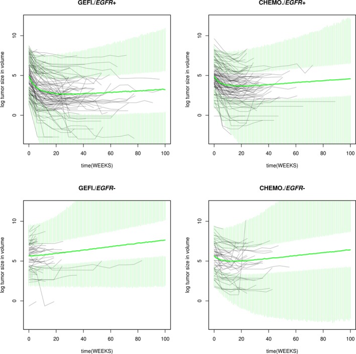
Observed and simulated tumor size profiles. CHEMO, chemotherapy; EGFR−, epidermal growth factor receptor negative; EGFR+, epidermal growth factor receptor positive; GEFI, gefitinib.

Figure 3.

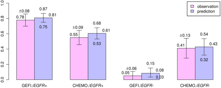
The percentage of patients achieving 30% shrinkage in sum of longest diameters. CHEMO, chemotherapy; EGFR−, epidermal growth factor receptor negative; EGFR+, epidermal growth factor receptor positive; GEFI, gefitinib.

Figure 4.

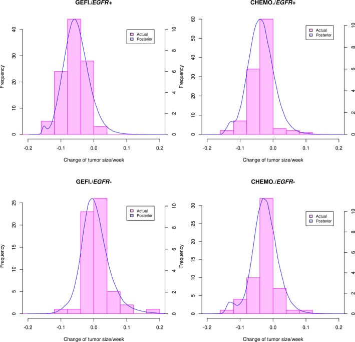
Observed and estimated percent initial change from baseline in sum of longest diameters per week. CHEMO, chemotherapy; EGFR−, epidermal growth factor receptor negative; EGFR+, epidermal growth factor receptor positive; GEFI, gefitinib.

Results

Summary statistics of the posterior distributions of the transformed parameters and key MCMC convergence diagnostics are shown in the Supplementary Information, indicating satisfactory convergence of MCMC. We performed the following checks to ensure that the model captures the key features of the data. The model described the dynamics of tumor size change in response to gefitinib or chemotherapy in the IPASS study well (Figure 2 and Table S2). The model simulation was performed through week 100. Note that the discrepancy between the summary distributions of the observation and the summary distribution of the posterior predictive samples increases as time increases (Table S2) because the model simulation does not account for the drop out of patients. The dynamic model adequately described individual patient tumor size as indicated by close agreement of observed and predicted individual measurements of tumor size at all time points and in all patients (Figure S2). Model predictions of the proportion of patients achieving more than 30% reduction of linear tumor size from baseline agree with the observed proportions as shown in Figure 3. These proportions parallel the observed differences in objective response rates (of which tumor size reduction from baseline is a key component) in the IPASS study.11 The model adequately described variation of tumor size among patients. The posterior distributions of each patient’s baseline tumor size in each group agrees well with the observed distributions (Figure S3). The model adequately captured the change from the baseline of tumor size, as shown by agreement of the posterior distribution of percent change from baseline and the observed distributions (Figure 4 and Table S3). This agreement holds for all treatments by EGFR mutation groups.

Summary statistics of the posterior distributions of untransformed model parameters estimated using data from the IPASS study are shown in Table 1. Posterior distributions of model parameters for each group are shown in Figure 5. Baseline tumor size is on average 118% larger in the EGFR‐positive than in the EGFR‐negative patients. The net growth rate of fully resistant tumors is the lowest at 0.01 per week and very similar for gefitinib‐treated and chemotherapy‐treated EGFR‐positive patients, whereas it is on average 76% larger for chemotherapy‐treated EGFR‐negative patients and 127% larger for gefitinib‐treated EGFR‐negative patients. Maximum drug effect on the net growth rate at the start of treatment is largest for gefitinib‐treated EGFR‐positive patients (0.31 per week), followed by chemotherapy‐treated EGFR‐positive and EGFR‐negative and gefitinib‐treated EGFR‐negative patients (0.04 per week). A slight difference in the initial effect for chemotherapy between EGFR‐positive and EGFR‐negative tumors (0.23 vs. 0.18 per week) may reflect differences in biology and sensitivity of the tumors to chemotherapy influenced by the presence of driving EGFR mutations. The rate of emergence of resistance is the lowest in EGFR‐positive patients treated with gefitinib (0.136 per week). The rate is 44% higher in EGFR‐positive patients treated with chemotherapy. The rate of resistance emergence in EGFR‐negative patients on chemotherapy is less certain and is consistent with the rates in EGFR‐positive patients (the posterior distribution is wider and overlaps the distributions for EGFR‐positive patients). The variance of the posterior distribution of the rate for EGFR‐negative patients treated with gefitinib is large, indicating that a wide range of rate values is consistent with the data. Such large variance of $\mathrm{\alpha }$ coupled with the small ${\mathrm{\Delta }}_{\mathrm{\lambda }}$ reflects the difficulty in estimating $\mathrm{\alpha }$ when tumors barely respond to treatment and start growing right away.

Table 1.

Parameter values estimated from clinical data

Parameter	Patients' group	Mean	SE_mean	SD	2.50%	25%	50%	75%	97.50%	n_eff	$\widehat{R}$
$\text{TV}\_Y_0\left({\text{mm}}^3\right)$	Gefi+	292.70	0.81	50.88	204.97	258.50	289.12	321.75	407.27	3940.3	1.00
	Ch+	292.70	0.81	50.88	204.97	258.50	289.12	321.75	407.27	3940.3	1.00
	Gefi−	133.94	0.28	17.75	101.69	121.58	132.86	145.12	171.19	4000.0	1.00
	Ch−	133.94	0.28	17.75	101.69	121.58	132.86	145.12	171.19	4000.0	1.00
$\text{TV}\_k_{\text{gr}}\left(\frac{1}{\text{week}}\right)$	Gefi+	0.0092	0.0000	0.0020	0.0060	0.0078	0.0090	0.0104	0.0136	2650.3	1.00
	Ch+	0.0101	0.0000	0.0022	0.0065	0.0085	0.0098	0.0114	0.0152	2558.4	1.00
	Gefi−	0.0227	0.0002	0.0081	0.0101	0.0166	0.0217	0.0274	0.0421	1322.2	1.00
	Ch−	0.0176	0.0001	0.0058	0.0088	0.0135	0.0167	0.0209	0.0309	2064.1	1.00
$\text{TV}\_\mathrm{\alpha }\left(\frac{1}{\text{week}}\right)$	Gefi+	0.1356	0.0003	0.0183	0.1036	0.1229	0.1341	0.1472	0.1757	3013.7	1.00
	Ch+	0.1956	0.0007	0.0340	0.1393	0.1714	0.1922	0.2160	0.2709	2531.3	1.00
	Gefi−	0.1810	0.0126	0.2728	0.0076	0.0503	0.1031	0.2000	0.8550	467.0	1.01
	Ch−	0.1838	0.0015	0.0628	0.0938	0.1396	0.1733	0.2174	0.3351	1759.9	1.00
$\text{TV}\_{\mathrm{\Delta }}_{\mathrm{\lambda }}\left(\frac{1}{\text{week}}\right)$	Gefi+	0.3099	0.0006	0.0335	0.2495	0.2864	0.3088	0.3320	0.3817	3490.6	1.00
	Ch+	0.2325	0.0006	0.0303	0.1773	0.2117	0.2307	0.2516	0.2970	2843.8	1.00
	Gefi−	0.0410	0.0011	0.0248	0.0136	0.0260	0.0355	0.0485	0.1038	517.3	1.01
	Ch−	0.1758	0.0008	0.0391	0.1132	0.1481	0.1713	0.1986	0.2651	2327.0	1.00

Δ_λ, the maximum intensity of the drug effect; α, the rate of resistance emergence; Ch+, EGFR positive patients treated with chemotherapy; Ch−, EGFR negative patients treated with chemotherapy; Gefi+, EGFR‐positive patients treated with gefitinib; Gefi−, EGFR‐negative patients treated with gefitinib; k _gr, the net tumor growth rate; n_eff, effective sample size; SD, standard deviations; SE_mean, Monte Carlo standard errors; TV, Typical value; Y ₀, the initial tumor volume.

Figure 5.

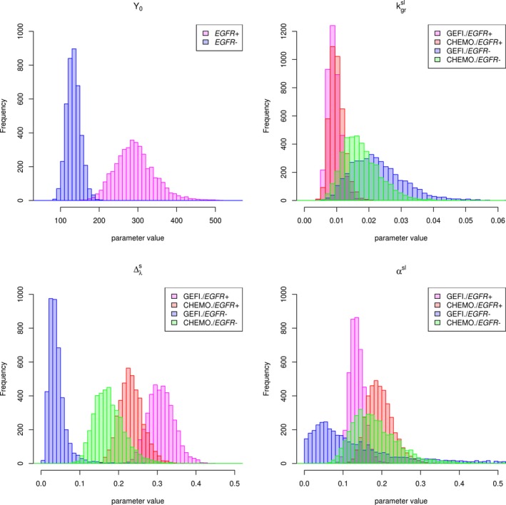
Posterior densities of model parameters. CHEMO, chemotherapy; EGFR−, epidermal growth factor receptor negative; EGFR+, epidermal growth factor receptor positive; GEFI, gefitinib; Y ₀, the initial tumor volume; $k_{\text{gr}}^{\text{sl}}$, the net tumor growth rate (scaled, log‐transformed); ${\mathrm{\Delta }}_{\mathrm{\lambda }}^s$, the maximum intensity of the drug effect (scaled); α^sl, the rate of resistance emergence (scaled, log‐transformed).

Discussion

The dynamic model for tumor size response to treatment allowed us to parse out differences in tumor size profiles, characterized by the pattern of initial response to treatment and the eventual regrowth of tumors among the treatment groups (Figure 2) in terms of differences in model parameters. The key characteristics of tumor size response are the magnitude of maximum decrease from baseline (i.e., depth of response or the nadir), time to nadir, and the rate of eventual regrowth. They are composite quantities of the elementary parameters maximum drug effect, rate of resistance emergence, and the net growth rate of fully resistant tumors. The largest maximum drug effect on the net growth rate and the smallest rate of emergence resistance in EGFR‐positive tumors treated with gefitinib underlie the superior tumor response in this subgroup when compared with chemotherapy in EGFR‐positive or EGFR‐negative tumors or gefitinib in EGFR‐negative tumors. The lower response to chemotherapy than gefitinib in EGFR‐positive tumors can be explained by the smaller maximum drug effect on the growth rate and larger rate of resistance emergence. The maximum drug effect is the following in decreasing order: gefitinib in EGFR‐positive, chemotherapy in EGFR‐positive, chemotherapy in EGFR‐negative, and gefitinib in EGFR‐negative tumors. The rate of resistance emergence is, in increasing order: gefitinib in EGFR positive, chemotherapy in EGFR positive, while each is plausibly similar to the rate in EGFR‐negative tumors, which are estimated with less certainty, which are estimated with less certainty. The rate of growth is smaller in EGFR‐positive than in EGFR‐negative fully resistant tumors, regardless of treatment. Figures 5 and 6 illustrate these relationships. This ranking of parameter values is consistent with the ranking of tumor response and progression‐free survival in these treatments and the EGFR subgroups.11 Thus, we hypothesize that larger ${\mathrm{\Delta }}_{\mathrm{\lambda }}$, lower $\mathrm{\alpha }$, and lower $k_{\text{gr}}$ will correlate with superior response in terms of progression‐free survival.

Figure 6.

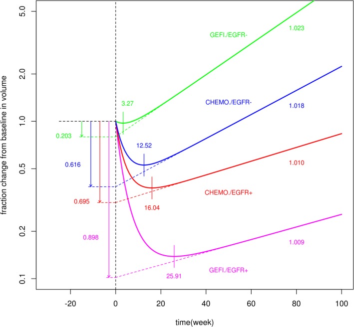
Typical sum of longest diameter profiles. CHEMO, chemotherapy; EGFR−, epidermal growth factor receptor negative; EGFR+, epidermal growth factor receptor positive; GEFI, gefitinib.

Recently, Mistry et al.16 used a linear population dynamics model to compare tumor response to gefitinib and chemotherapy. Their model included a resistant and sensitive population of cancer cells. Resistant cells had a positive net growth rate, and sensitive cells had a negative net growth rate. They concluded that in a first‐line setting (the IPASS study), chemotherapy led to a smaller regrowth rate than gefitinib in the overall population of EGFR‐positive and EGFR‐negative patients. They used the acquired resistance version of the model for chemotherapy and a de novo version of the model for gefitinib. In the acquired resistance version of the model, sensitive cells transformed into resistant cells with a linear rate. In the de novo model, a preexisting proportion of resistant cells that do not change on treatment was estimated. In contrast, using our model with a model of resistance emergence common to different drugs, we provide a more precise interpretation of the difference of tumor response between gefitinib‐treated and chemotherapy‐treated patients. (Identification of the de novo vs. acquired models is difficult given that only the total volume of the tumor is measured, and the two models in Mistry et al.16 are mathematically equivalent up to a different parameterization). The regrowth rate is similar for gefitinib and chemotherapy in either EGFR‐positive or EGFR‐negative tumors, whereas the difference in the overall tumor profiles arises because gefitinib has larger initial drug effect on the net growth rate and a lower rate at which the drug effect wears off (i.e., resistance emerges).

Estimating parameters of our tumor size dynamic model using tumor size response data in early trials will enable predictions of relative survival benefit and understanding of the reasons underlying them. Using our linear model (i.e., exponential growth or decline of tumor size) is appropriate given the typically small range of tumor size change in clinical trials where tumors are not allowed to grow unrestricted to show the saturation of growth as in Gompertz or logistic growth. Predictions can be performed either for the rate and extent of tumor regrowth (tumor progression) using the dynamic model or survival using a joint model of tumor size dynamics and survival.6 Using the same structure of the model for different investigational treatments in the same type of cancer and a Bayesian approach will facilitate modeling and the interpretation of tumor size data from early trials. In this case, a Bayesian model developed on a large data set and many drugs will be reestimated with data from a small trial of an innovative investigational treatment, providing better estimates for its effect on tumor dynamics.

Funding

This study was sponsored by AstraZeneca Pharmaceuticals.

Conflict of Interest

M.N., A.S., Y.H., J.D., and N.A‐H. are employees of AstraZeneca Pharmaceuticals LP.

Author Contributions

All authors wrote the manuscript. M.N. and S.A. designed and performed the research. M.N. analyzed the data.

Supporting information

Figure S1. Approximation by cubic of sum, scaled by 10‐9 for this figure.

Figure S2. Observed sum of longest diameters (SLD) (mm) vs. median of posterior distribution of each measurement.

Figure S3. Observed and estimated initial tumor size (in mm³): The histograms (pink) are actual measurements for the initial log tumor size (at time 0), and blue lines represent the posterior density of median value for the log tumor size drawn from the posterior samples.

Figure S4‐1. Markov chain trace plot of Y0: The plot provides a visual way to inspect sampling behavior and assess mixing across chains and convergence. No autocorrelation (randomly sampled) indicates that the samples were well drawn.

Figure S4‐2. Markov chain trace plot of k _gr.

Figure S4‐3. Markov chain trace plot of Δ.

Figure S4‐4. Markov chain trace plot of α.

Figure S5‐1. Energy plot of Y ₀: Correlations between the sample of model parameters and energy. No correlation between them indicates that the samples were well drawn.

Figure S5‐2. Energy plot of k _gr.

Figure S5‐3. Energy plot of Δ.

Figure S5‐4. Energy plot of α.

Table S1. Approximation by cubic of sum.

Table S2. Summary distribution, observation vs. posterior predictive samples.

Table S3. Summary distribution of percent initial change (baseline to 6 weeks, fraction change per week).

Table S4. Transformed parameter values estimated from clinical data.

References

- 1. Howlander, N. et al SEER cancer statistics review, 1975‐2016 (National Cancer Institute, Bethesda, MD, 2019). [Google Scholar]
- 2. Ernani, V. , Steuer, C.E. & Jahanzeb, M. The end of nihilism: systemic therapy of advanced non‐small cell lung cancer. Annu. Rev. Med. 68, 153–168 (2017). [DOI] [PubMed] [Google Scholar]
- 3. Lynch, T.J. et al Activating mutations in the epidermal growth factor receptor underlying responsiveness of non‐small‐cell lung cancer to gefitinib. N. Engl. J. Med. 350, 2129–2139 (2004). [DOI] [PubMed] [Google Scholar]
- 4. Sim, E.H. et al Gefitinib for advanced non‐small cell lung cancer. Cochrane Database Syst. Rev. 1, CD006847 (2018). [DOI] [PMC free article] [PubMed] [Google Scholar]
- 5. Eisenhauer, E.A. et al New response evaluation criteria in solid tumours: revised RECIST guideline (version 1.1). Eur. J. Cancer 45, 228–247 (2009). [DOI] [PubMed] [Google Scholar]
- 6. Brilleman, S.L. et al Joint longitudinal and time‐to‐event models for multilevel hierarchical data. Stat. Methods Med. Res. 28, 3502–3515 (2019). [DOI] [PubMed] [Google Scholar]
- 7. Rizopoulos, D. Dynamic predictions and prospective accuracy in joint models for longitudinal and time‐to‐event data. Biometrics 67, 819–829 (2011). [DOI] [PubMed] [Google Scholar]
- 8. Claret, L. et al Model‐based prediction of phase III overall survival in colorectal cancer on the basis of phase II tumor dynamics. J. Clin. Oncol. 27, 4103–4108 (2009). [DOI] [PubMed] [Google Scholar]
- 9. Ribba, B. et al A review of mixed‐effects models of tumor growth and effects of anticancer drug treatment used in population analysis. CPT Pharmacometrics Syst. Pharmacol. 3, e113 (2014). [DOI] [PMC free article] [PubMed] [Google Scholar]
- 10. Laird, A.K. Dynamics of tumor growth. Br. J. Cancer 13, 490–502 (1964). [DOI] [PMC free article] [PubMed] [Google Scholar]
- 11. Mok, T.S. et al Gefitinib or carboplatin‐paclitaxel in pulmonary adenocarcinoma. N. Engl. J. Med. 361, 947–957 (2009). [DOI] [PubMed] [Google Scholar]
- 12. Carpenter, B. et al Stan: a probabilistic programming language. J. Stat. Softw. 76 (2017). [DOI] [PMC free article] [PubMed] [Google Scholar]
- 13. Stan Development Team . RStan: The R interface to Stan. R package version 2.17.3. <http://mc‐stan.org> (2018). [Google Scholar]
- 14. R Core Team . R: A Language and Environment for Statistical Computing (R Foundation for Statistical Computing, Vienna, Austria, 2019). [Google Scholar]
- 15. Arai, T. et al Tumor doubling time and prognosis in lung cancer patients: evaluation from chest films and clinical follow‐up study. Japanese Lung Cancer Screening Research Group. Jpn J. Clin. Oncol. 24, 199–204 (1994). [PubMed] [Google Scholar]
- 16. Mistry, H.B. et al Resistance models to EGFR inhibition and chemotherapy in non‐small cell lung cancer via analysis of tumour size dynamics. Cancer Chemother. Pharmacol. 84, 51–60 (2019). [DOI] [PMC free article] [PubMed] [Google Scholar]
Associated Data
This section collects any data citations, data availability statements, or supplementary materials included in this article.
Supplementary Materials