Acceleration of spleen segmentation with end-to-end deep learning method and automated pipeline

Abstract

Delineation of Computed Tomography (CT) abdominal anatomical structure, specifically spleen segmentation, is useful for not only measuring tissue volume and biomarkers but also for monitoring interventions. Recently, segmentation algorithms using deep learning have been widely used to reduce time humans spend to label CT data. However, the computerized segmentation has two major difficulties: managing intermediate results (e.g., resampled scans, 2D sliced image for deep learning), and setting up the system environments and packages for autonomous execution. To overcome these issues, we propose an automated pipeline for the abdominal spleen segmentation. This pipeline provides an end-to-end synthesized process that allows users to avoid installing any packages and to deal with the intermediate results locally. The pipeline has three major stages: pre-processing of input data, segmentation of spleen using deep learning, 3D reconstruction with the generated labels by matching the segmentation results with the original image dimensions, which can then be used later and for display or demonstration.

Given the same volume scan, the approach described here takes about 50 s on average whereas the manual segmentation takes about 30min on the average. Even if it includes all subsidiary processes such as preprocessing and necessary setups, the whole pipeline process requires on the average 20 min from beginning to end.

1. Introduction

Computed Tomography (CT) is widely used in clinical medicine to detect anatomical abnormalities inside of the human body. CT provides 3D structural information that enables assessment of tissues within organs. As this information is inherently digital, it can be used for both qualitative and quantitative assessment. Despite this capability, various drawbacks pertaining to quantitative imaging and disadvantages of CT imaging still hamper the use of quantitative CT information for clinical care, and complicate research [2–5]. Projection of the CT image invokes technical limitations, and the inconvenient workflow of knowledge generation from the imaging data limit efficiency. Here, we focus on spleen tissue as an example of the segmentation of organs from abdominal CT image. Spleen volume is used for both clinical and pharmacological purposes. Clinically, abnormal spleen volume has important diagnostic value in the diagnosis of liver diseases, blood cancer – specifically myeloproliferative neoplasms and lymphomas - infections and some forms of anemia [6,7]. Pharmacologically, spleen volume can be a dosage indicator for prescription or for the assessment of drug effectiveness after administration and planning of surgical procedures.

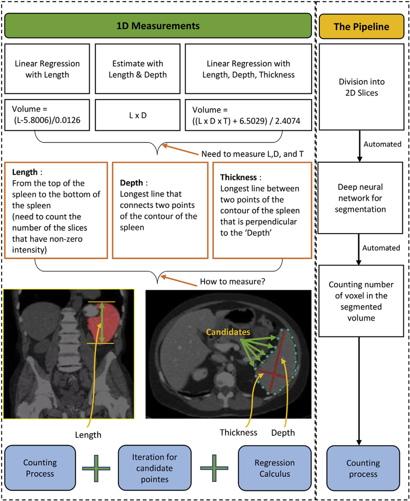
Currently, numerous methods have been utilized for measuring spleen volume and assessing anatomical diseases through the measurement [8,9]. Among them, linear regression [1] and deep learning [10] are the most commonly used methods for spleen segmentation and volume estimation (Fig. 1). Linear regression requires the clinician to make an initial, correct estimate of a size parameter and 2D measurements such as the spleen length, depth, and thickness [1,11]. Deep learning has issues with intermediate and subsidiary results such as resampled scans and 2D sliced image set. For these methods to provide a good volume estimate, accurate manual labelling of voxels is required. In addition, deep learning requires manual interventions at some intermediate steps (Fig. 1). Manual segmentation is time consuming and has results that vary between radiologists [12]. Fast automatic segmentation algorithms with consistent results would be of considerable value. This work improves state of the art Deep Learning through the use of an end-to-end pipeline that automates the spleen segmentation and volume estimation.

Fig. 1.

Current methods for measuring spleen volume biomarker. Left box includes three fundamental methods which are linear regression with measured spleen length, length multiplied by depth, and linear regression with spleen length, depth, and thickness [1]. Right box shows our pipeline method that will resolve and improve the issues in current methods and accelerate intermediate processes and reduce manual works significantly.

From the traditional research perspective, the data preparation from a 3D volume to a set of 2D slices and a volume reconstruction after segmentation requires more time than the segmentation itself. First, 3D CT images must be transformed into 2D slices for segmentation because most deep neural networks require 2D, not 3D, images to be trained and validated [13]. In pre-processing, slices must be resized and intensity-normalized by image processing algorithms so that all the input data has the same dimensions and intensity range. Lastly in post-processing, segmented slices have to be re-converted into 3D images whose dimensions are same as original input. Since subsidiary results derived from each sub-process often must be ported between different software packages (and sometimes even operating systems), researchers must spend time to process the data in terms of resampling that could be better used in other ways. However, these steps are essential for the deep learning method.

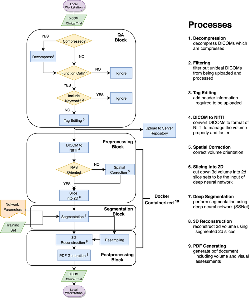
Here, we propose containerizing tools to overcome these issues. (By containerization, we mean automatically concatenating all the procedures involved in segmentation with a virtual machine so that they can be performed without manual piecewise management of the data flow.) Docker, one of the most commonly used containerization programs, enables program execution without explicit system specifications [14]. Using Docker, we combined the whole pipeline process into one script file that requires neither function calls nor script processing apart from the Docker script. We describe the following parts: Data decompression, Data push and uploading, Pre-processing, Segmentation, and Postprocessing (Fig. 2), the methods used by each process, and their intermediate results. The spleen volume estimated through the entire pipeline, end-to-end, is displayed within a PDF document which clinicians can use for subsequent documentation.

Fig. 2.

Overall system pipeline. It contains general processing steps from local data preprocessing to retrieving the labeled spleen volume back to the local machine.

The pipeline is described end-to-end in Fig. 2. A quality assurance (QA) process is composed with raw data preparation and filtering. Clinical systems often use data compression, but research systems generally do not support it well. Thus, data from clinical files must be decompressed before its use. The header information of the decompressed DICOM, which is ‘Patient Comments’, is edited to add the information: Project ID, Subject ID, and Session ID. That is followed by keyword and functional filtering processes as a quality assurance. In Fig. 2, the main container includes three procedures. At the preprocessing block, DICOMs are converted into NIfTI [15], spatially orientation corrected, and converted into a set of 2D slices. The sliced images are input into a segmentation process, called SSNet [10,16,17], that uses a deep neural network. After segmentation, the slices are merged and overlaid with 3D volumetric labels. Finally, the pipeline generates a PDF file that shows auto-volumes, 3 views (axial, coronal, sagittal), and a 3D rendered image. These main parts of the system are composed in Docker container.

2. Methods

2.1. Data preparation

In this paper, for data loading, both local and through the internet, we selected DCMTK toolkit from OFFIS [18]. The DICOM research library introduced with [18] can detect, but not read, compressed DICOMs. Since DICOM files are normally compressed to reduce size as JPEG 2000 format, decompression must precede any other processes. The DCMTK function, ‘dcmdjpeg’ detects compressed DICOMs and converts them into uncompressed DICOM (“.dcm”) format files.

The DICOM header information varies across scanner types. Therefore, to upload CT data or to send it to a repository, a common tag should be fixed or edited by users. This study uses the target repository, XNAT, which is operated by VUIIS Center for Computational Imaging (VUIIS CCI) at Vanderbilt University [19]. Also, to send CT DICOMs to XNAT, a tag (0010,4000), ‘Patient Comments’, is required. So, if it is missing, we add it. We tested our procedure with data from three scanners - Siemens, Philips, and GE - among the most widely used. It is the case that even if the data are taken from the same model of scanner, some have the tag (0010,4000) while others do not. Therefore, we created a function to edit the tag (0010,4000) for the DICOMs which have passed ‘Quality Assurance’ before our segmentation procedure begins. The tag ‘Patient Comment’ is edited or added as the key header and the server will detect this header in each scan.

2.2. Quality assurance and push to server

Ahead of the tag editing procedure, our system tests the validity of the included scans. Invalid scans include: not a real image, missing any of the three-view images (axial, coronal, sagittal), or scans that have inappropriate scan thicknesses such as 0.1mm or 15 mm. These are filtered out to prevent faulty or spurious data from being uploaded to the repository. Since any DICOM image has relevant specific headers such as ‘Scan Options’ and ‘Slice Thickness’, the data can be filtered using these keywords. There are two representative scan options which must be filtered out - ‘DOSE’ and ‘SCOUT’. The Dose report only includes text descriptions, not an image volume. The Scout view cannot be used because the contrast of the scout image does not include the contrast medium. Only the filtered scans are header-commented by the manipulation of the common header information, which is (0010, 4000), ‘Patient Comments’. First, the DICOM CT data is filtered using ‘Functional QA’ before the commenting process. This ‘Functional QA’ is conducted by python library function pydicom. Some faulty images are detected by the python library function read_file() function, which returns an exception related to the specific fault. The function mainly plays a role at filtering header bad files in terms of header information. For instance, read_file() removes header information-omission cases, deprecation of header information. When the function finds improper files, it returns message which is ‘File is missing DICOM File Meta Information” “header or ‘DICM’ prefix is missing from the file’. Upon passing the functional QA, a keyword filtering process is applied to further remove faulty scans in terms of scan types and slice thickness. In the meantime, the keyword ‘Slice thickness’ has a criterion that varies depending on the person. The proper range of thickness can be determined empirically by balancing diagnostic contents in the image and image noise [20]. Thicker the slice is, more partial volume artifact it has in the image. Then the data can be filtered with specific ranges of slice thickness [20]. The designated slice thickness range for this QA is in the interval (0.5, 6.0) mm which does not have significant difference of the image noise [20] and helps to keep as much as training set with over-whelming performance comparing to manual segmentation. Setting the slice thickness interval as (0.5, 6) mm, we could see that the pipeline segmentation surpasses the performance of manual segmentation and also almost all the Dicom files included in 185 scans could be used, only except about 20 Dicom files. If the image has passed both functional and keyword quality assurance, the tag (0010,4000) will be edited for uploading data to the target server as described in Table 1.

Table 1.

DICOM headers (tags) for identifying and qualifying targets to be processed. Scan Option and Slice Thickness headers are used to filter out the unintended data. Patient Comments, which is (0010,4000), is the target header that is modified or edited to be uploaded to the server. All three scanners we used in the study (Siemens, Philips, and GE) have the ‘Scan Options’ and ‘Slice Thickness’ header, but as for the ‘Patient Comments’, they do not. We used this header to specify the directory and location of the data at the server since they can include most essential information of the DICOM files: Project ID, Subject ID, and Session ID.

Tag	Description	Value
(0018, 0022)	Scan Options	Ex: Helical Mode,
		Dose Report, Scout Image
(0018, 0050)	Slice Thickness	Float number variance
(0010, 4000)	Patient Comments	‘ProjectID-SubjectID-SessionID’

After header tag editing, the DICOM file is stored in the repository, ready to be reported and used for later cases and experiments. XNAT is a server that the user-defined system pipeline can work with automatically for the use-created project. The python command, python storescu.py -aec AE server port connects to the XNAT server and uploads the DICOM file. AE is the application entity title, and DICOM SCP is the server host name with port number. The command returns the server connection status, and the result of the upload via a system message.

2.3. Preprocessing

To facilitate the processing of the spleen imagery and subsequent management of the data, the pipeline converts a DICOM formatted document into NIfTI format, which has a header for 3D volumetric images. Since the Deep Neutral Network (DNN) used here operates on 2D images, the NifTI format 3D image must be converted into a set of 2D slices.

The voxels in clinical data may not have consistent dimensions or orientations, which can cause segmentation to fail. Therefore, the 3D image must be normalized via spatial correction functions beforehand. In the original image, a principal direction is selected. The volume is sliced perpendicularly to partition it into a set of 2D images. In this case, a set of equally spaced parallel planes, perpendicular to the principal direction are selected, and voxels between any two planes are projected onto a plane to form one 2D slice. During or after projection each image is resampled to conform to the DNN being used. For this work, the network requires 512 × 512 images for training and validation. Moreover, a CT image has its own orientation. To train the DNN, this orientation has to be the same across all the input scans and across all the training data i.e. the principal directions for slicing must be consistent with the spleen’s anatomy. Once the data is normalized a Right, Anterior, Superior (RAS) coordinate system is used for the deep learning process since RAS is particularly useful for matrix and vector math, where a right-hand coordinate system is customarily used (though a left-hand system can be used with appropriate adjustments) [21].

2.4. Deep spleen segmentation

After preprocessing the 3D data into a set of metrically consistent 2D images, we segmented it into spleen/not-spleen regions using the DNN described in Refs. [10,16,17,22] which is based on ResNet [23]. DNN segmentation alone may be insufficient for accurate spleen volume estimation. For example, image quality may be compromised. A small training set, metric and intensity variations, and anomalies such as spurious features introduced during preprocessing can degrade the volume. To address the problem, we implemented image processing algorithms, especially noise filtering [11,24]. After image processing, the 2D images must be reconstructed into a 3D volume that matches the dimensions and orientation of the original input. The denoising processes and additional correcting methods are mentioned in section 2.5.

2.5. Morphological correction

The errors in segmentation to be corrected via post processing include holes in segmentation, uneven edges, and rough labeling. Many of those errors can be corrected with morphological processing of the segmentation mask. (A segmentation mask is a binary image that indicates which pixels or voxels belong to the object and which do not.) The mask was processed with morphological opening, and a function, get_largest_connection(), which plays a role of counting the number of adjacent voxels and gives a same label to connected voxels, followed by closing [24]. Especially, the function get_largest_connection() changes voxel which has less than threshold amounts of non-zero voxel around itself. They remove the majority of the noise and make contours of segmentation smoother with little loss of information.

2.6. Containerization

The entire pipeline processes above is relocated into a large container that executes those previous steps end-to-end. Docker, a container platform that provides application to users to access across the hybrid cloud, enables this integration [14]. To run the pipeline, there are a number of data requirements and pre-installation processes needed; preprocessing and post-processing functions are performed by MATLAB codes, and the segmentation is done by Pytorch. Moreover, since the machines or Operating Systems (OS) vary across clinicians or users, the system environment must be unified. These required packages and OS are often more than some gigabytes in size, thus it can be cumbersome and time-consuming for a user to search for and install those packages. However, Docker can substantially cut down the time spent in such installations. A ‘Dockerfile’ script has commands and code lines for the installation of the requisite background systems; it sets up the system environments and required software packages on the virtual machine that executes the Docker code. Hence, Docker allows the automated pipeline to be released to users so that they can directly run the pipeline, with no requirements, other than installing the Docker software on their machine.

3. Evaluation

3.1. Dataset

The clinical trial that is being used in the paper to test the pipeline is the set of CT image data from ‘A Phase 1 Dose Escalation and Expansion Study of TGR-1202 + Ruxolitinib in Subjects with Primary Myelofibrosis (PMF), Post-Polycythemia Vera MF (PPV-MF), Post-Essential Thrombocythemia MF (PET-MF), MDS/MPN, or Polycythemia Vera Resistant to Hydroxyurea’ [26] (NCT02493530) that obtained IRB approval. Our subset of the CT trial consists of 185 scans from 56 subjects in anonymized form. Before the QA process, the protocol has data that should be filtered out so it does not enter the pipeline process.

3.2. Results

The automated pipeline showed good performance in general. For some subjects, partial regions of their spleens were mislabeled after being processed by the pipeline, so that additional manual labeling was necessary. After additional manual labeling, the segmentation result with the volume overlaid was evaluated by a radiologist. Despite the manual corrections to labels, the time expended for segmentation with the pipeline was still much less than purely manual labeling. Moreover, the results of the automated pipeline correspond closely to the manual segmentation.

3.2.1. Segmentation time

Traditionally, spleen segmentation -of clinical trial CT volumes has been done manually. To compare the manual segmentation to the auto-segmentation via pipeline, the manual labeling speed must be calculated first. For example, a scan, with 73 slices of spleen segments was manually labeled, and the elapsed time measured. Ignoring pauses in the procedure (e.g., rest time for the person doing the segmentation), the elapsed time was 24 min. The average manual segmentation speed was 20 s per slice. For the entire dataset, which has 185 scans and 10,552 slices with spleen tissue in them, the total manual segmentation time ignoring pauses was approximately 3517 min – almost 59 h in total.

The pipelined procedure, excluding the DNN, was performed on an, Intel(R) Xeon(R) CPU E5–1620 v3 @ 3.50 GHz 64 bit with 256 GB memory capacity. The DNN was computed on a Nvidia -GEFORCE GTI 1080 Ti GPU. The automated process without any additional manual labeling, took 1659 min for a total of 185 complete CT-scans. Manual editing of the 36 scans that had label errors took 416 min. Therefore, in total, the auto-pipeline with supplementary manual editing took 2075 min compared to the 3517 min required for fully manual segmentation. Considering that fully-manual labeling requires work breaks and that the hardware performance can be improved 3517 min is a lower bound on manual segmentation and 2075 min is an upper bound on the pipelined approach.

3.2.2. Quantitative analysis

After running the pipeline, we compared estimated spleen volume from our pipeline method and the volume from the linear regression equations given in Refs. [1,9]. Therein, spleen volume is estimated using the length (L), depth (D), and thickness (T) of the spleen. L is measured as vertical distance from the top of spleen to the bottom of spleen, D is from the longest line that connects two points on the contour of the spleen of the axial scan at the median slice of the volume, and T is computed by finding the longest line in the same slice as the depth that is perpendicular to the depth. Two linear regression equations introduced by Refs. [1,11] for evaluation are,

$$\text{Volume}[\text{cc}]=((\text{Length}{(\text{cm})}^{*}\text{Depth}(\text{cm})*\text{Thickness}(\text{cm}))+6.5029)/2.4074,$$ (1)

$$\text{Volume}[\text{cc}]=(\text{Length}(\text{cm})-5.8006)/0.0126$$ (2)

Eq. (1) estimates the spleen volume from three 1-D measurements, and Eq. (2) estimates it from a single 1-D measurement (Length). Our pipeline volume estimate is calculated by counting the number of the voxels which are labeled as ‘spleen’ through neural network multiplied by the volume of a single voxel. For comparison, we set the ground truth as the pipeline labeled volume followed by additional manual editing. The manual editing processes are performed by trained technologist, and the targets for manual correction were the scans/slices which are evaluated by radiologist as ‘slightly degraded’ and ‘very degraded’ after assessment of the initial method segmentations. A standard method for analysis is the correlation score of each method with the ground truth.

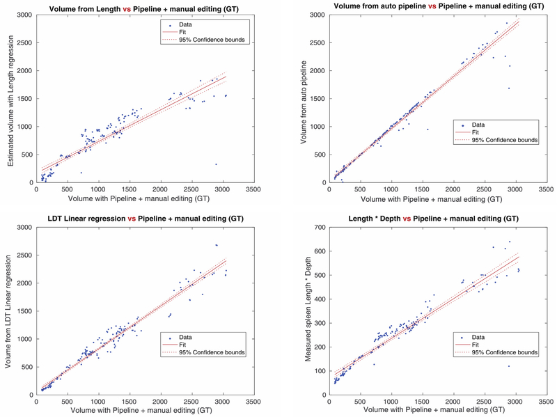
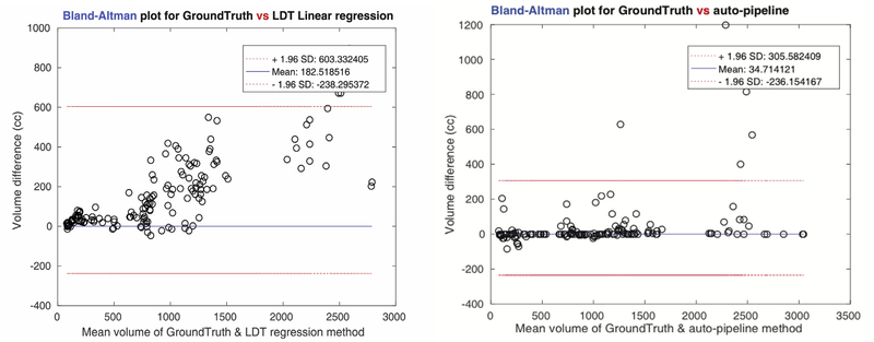
Fig. 3-(a) shows the correlation map for the all input scans used in our experiments. Linear regression with the measured spleen length gave us 0.9151 of correlation with the ground truth- the lowest degree of accuracy. The L multiplied by D method returned 0.9447, and L, D, T regression gave 0.9817 which was the highest among three previous methods. Our pipeline showed 0.9848 correlation- higher than any other methods. Moreover, the variance of the estimated spleen volume differences, according to the Bland-Altman plots in Fig. 3-(b), was significantly lower in our pipeline (471 cc), those of the linear regression methods (826 cc).

Fig. 3a.

Correlation score map for each regression and estimation method, and the pipeline method. Correlation scores from each method are 0.9151(Top left, Linear regression with Length), 0.9447(Top right, Length x Depth estimate), 0.9817(Bottom left, Linear regression with Length, Depth, and Thickness), 0.9848(Bottom right, the pipeline method with deep learning). The pipeline method shows the highest correlation score among the volume measurement methods.

Fig. 3b.

Bland-Altman plots for two cases (Length, Depth, Thickness regression, and the pipeline). Since among three linear regression methods, volume estimate with the Length, Depth, Thickness showed the best correlation, its performance is compared to the pipeline method. The volume difference is remarkably smaller at the pipeline method (variance of estimated volume difference = 471) than at the L, D, T regression (variance of estimated volume difference = 826).

3.2.3. Qualitative analysis

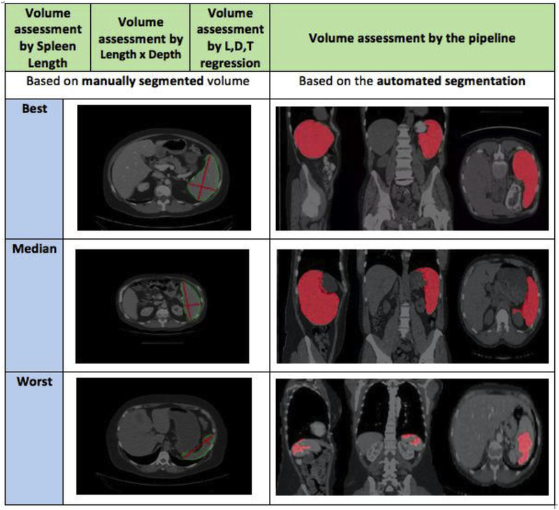
The pipeline performance can also be evaluated by comparing the worst case from the pipeline with other methods. Fig. 4 represents the qualitative results of the paper. It compares a traditional regression method with our pipeline method. Since the regression method considers only the length, depth, and thickness of the spleen at the location of the slice that contains the longest straight line within the whole spleen volume, the result can be affected considerably by the actual shape of the spleen in the CT scan. Even though the selected slice contains the longest line, that slice does not necessarily have the largest area. There are many different spleen shapes (therefore actual volumes) that have the same LDT estimate. Thus, various shapes of the spleen from different patients can result in large differences between estimated volume and the actual volume. The pipeline method, however, counts the number of voxels in the segmented volume. So, our procedure’s volume difference and variance are relatively lower than regression methods independent of the shape of the spleen. In Fig. 4, even though the estimated 1D measurements look reasonable, the slices that represent length, depth, and thickness are not indicative of the true volume.

Fig. 4.

The qualitative result of 1D measurement volume assessments and automated pipeline assessment. Measurement of the L,D, and T is done by trained technologists and evaluated by radiologist afterward (re-measured if assessment were ‘very degraded’ or ‘slightly degraded’. The quality of 1D measurement methods largely depends on the spleen volume shape since the spleen Depth and Thickness is determined in the slice which has longest connecting line from one point of the spleen to the other point of the spleen. Although 1D measurement figures look reasonable, the slice that is considered can be wrong and arise large difference of volume measurement. Automated pipeline method also has some bad cases that does not represent spleen correctly, but the pipeline method has lower volume error overall since it counts actual number of voxels for measuring volume.

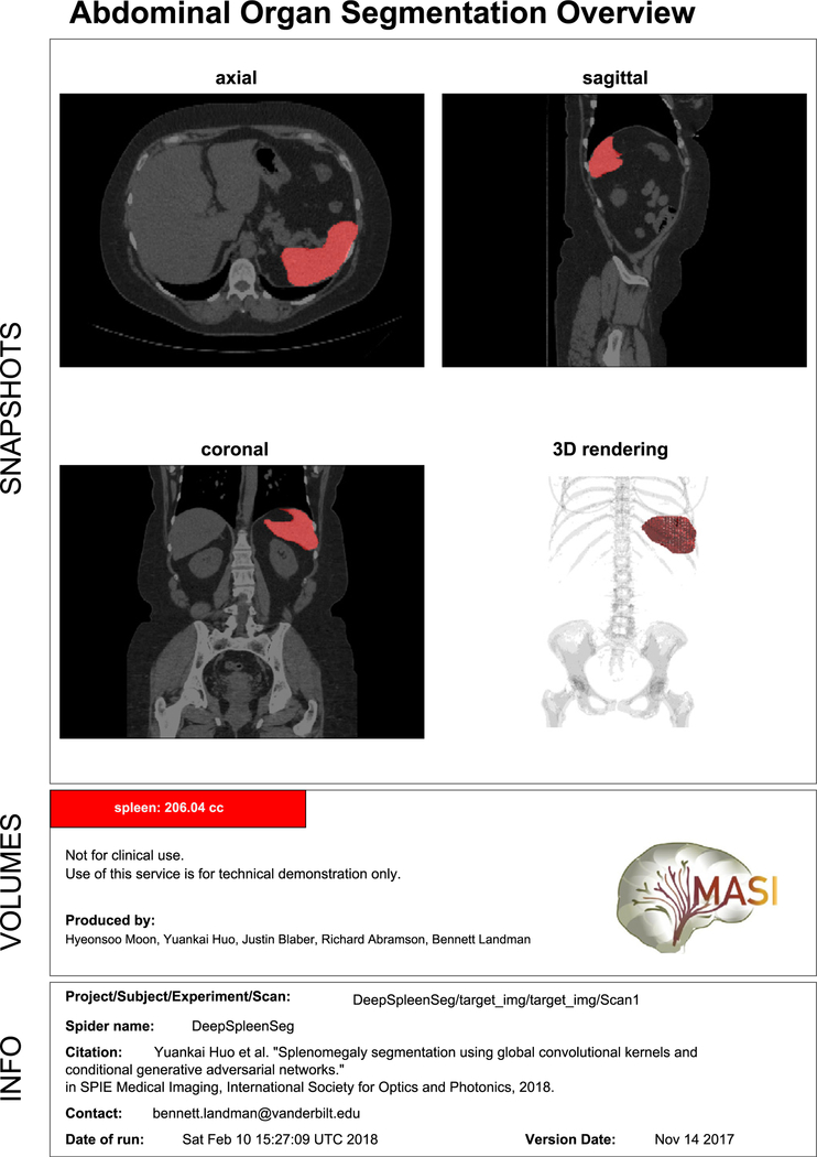
Fig. 5 shows one example of the final overview that clinicians and patients can obtain directly from the result of the end-to-end pipeline. Fig. 5, also shows the PDF overview that includes slice capture of the overlaid scan so that users can easily see and assess the result of the segmentation. It also displays the spleen volume calculated as the sum labeled voxels in the segmented image times the volume of a single voxel.

Fig. 5.

PDF Output for demonstration purposes. The PDF format includes three sections mainly. Snapshots section describe axial view, sagittal view, coronal view of mean slice, and rendering of 3D volume. Volume section shows brief description and actual spleen auto-volume from the pipeline. Info section has scan information and assessment data.

Fig. 6 illustrates the sensitivity and robustness of the pipeline. The correlation map and the Bland-Altman plots are only for the scans that were manually corrected after segmentation via the pipeline processes. Even restricted to the scans that had required additional manual editing, the pipeline showed sufficient accuracy. Although the correlation of those scans was lower than the regression volume estimation, the Bland-Altman plot showed better performance in terms of lower variance and differences among the volumes.

Fig. 6.

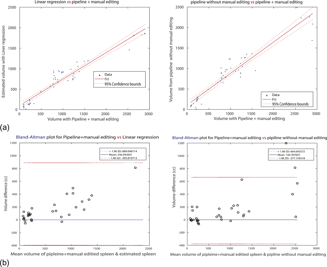
Robustness of the pipeline. It shows correlation score and Bland-Altman volume differences only for the scans that are ‘manually edited’ after running the pipeline process. (a) Represents correlation map for left: spleen volume from linear regression estimation and spleen volume from the pipeline with manual editing (GT), and right: spleen volume from the pipeline and GT. X-axis for both plots is the group evaluated as all ‘good’ by radiologist. It is remarkable that for the large spleens, the pipeline method shows degraded performance. (b) Introduces Bland-Altman plots for both two cases. It can be verified that the difference gap of linear regression estimated volumes is bigger (wider) than the pipeline method.

4. Discussion

The pipeline with deep learning method shows fast and accurate segmentation of spleen compared to traditional 1-D measurement methods. Moreover, containerized pipeline reduces processing time of subsidiary data format so that this work improves deep learning method for segmentation significantly in terms of fast processing and user convenience. However, the pipeline has few issues that should be discussed and can be further improved.

4.1. Volumetric issue

The volumetric problems can be identified with outliers in the correlation map, and also with the numerical value generated through the pipeline. We found that the pipeline can generate imperfect labels for some scans for two reasons. First, the number of training sets used in the pipeline for labeling is too small and specific. In the set of 185 images that we used, only 19 showed splenomegaly - an insufficient number for training of a DNN [21]. This was especially pronounced when the oversized spleen was larger than 1500 cc. We did not implement robust augmentation on this except subsampling from enlarged image (zero-padded) because excessive augmentation compared to the number of actual dataset could harm generality of the original dataset. The other reason is the wide variation in normal spleen sizes and shapes. Both issues could be resolved with larger training sets. For greatest accuracy in machine learning and recognition, the size of training dataset should be larger than the test dataset. The most widely used ratio is 70% for the training set, and 30% for the test set. We used a training set of 94 images (comprising 75 normal spleens and 19 with splenomegaly) with a test set of 185 scans that are in the 56 clinical trial subjects.

4.2. Future work

One of the problems we encountered was the misclassification of a small subset of voxels. They required manual editing to correct. Further studies could elucidate the causes of such misclassifications and suggest techniques for improving the results automatically. Increasing the size of the training set is expected to improve segmentation accuracy but that would also require experimentation to find an ideal learning rate for the DNN [25]. Modifications in the learning rate should be analyzed in relation to the size of the training set.

In this work, we evaluated the performance of the pipeline by comparing the estimated spleen volume with a previously published linear regression method. As [1] asserts, the measured length, depth (perpendicular to hilum, maximum on any section), and thickness (perpendicular to depth, maximum on any section), can be used to estimate the spleen volume [1]. The pipeline method could be evaluated further by comparing it to the estimated spleen volumes from different linear regression equations, such as ‘Volume [cc] = 30 + 0.58 × L (cm) × D (cm) × T (cm)’ proposed in Ref. [9], or by using additional index information like depth and thickness.

5. Conclusion

Current methods of spleen volume estimation are time and labor intensive. Data formats are inconsistent and image segmentation must be done by hand. The workflow can be complicated and inconvenient. To improve the situation, we have devised an end-to-end automated process using a Docker container. We showed a significant reduction in processing time while maintaining and in some cases exceeding the quality of the segmentation thereby providing a more accurate spleen volume estimate. Our emphasis on the automation of manual tasks improved the processing time. We have shown that our results represent a baseline since faster hardware will further reduce the time with no other changes to our automated pipeline. The end-to-end system described here, combined methods from pre-processing (DICOM header editing, Quality Assurance, slicing 3D volumes into set of 2D slices), automatic segmentation (based on SSNet using ResNet network and GAN), and post-processing (Image processing; Closing, Opening, 3D reconstruction, PDF demonstration). All the subsidiary and intermediate outputs such as 2D slices, resized dimensionality images, and labeled scans are saved in sub-directories so that no information is lost at any step. The final output is a single PDF document that contains the segmented 3D volumetric imagery, an estimate of the spleen volume, and all supporting documentation. We found the Docker container to be an ideal method to implement the autonomous segmentation and measurement for use by other researchers and clinicians. Although further studies that include larger training sets and more evaluation techniques could improve upon our results. The containerized, autonomous pipeline proposed in this work if used as is, significantly improves upon the current state of the art in spleen volume measurement.

References

- [1].Bezerra AS, et al. , Determination of splenomegaly by CT: is there a place for a single measurement? Am. J. Roentgenol 184 (5) (2005) 1510–1513. [DOI] [PubMed] [Google Scholar]
- [2].Sharma N, Aggarwal LM, Automated medical image segmentation techniques, Journal of medical physics/Association of Medical Physicists of India 35 (1) (2010) 3. [DOI] [PMC free article] [PubMed] [Google Scholar]
- [3].Rosenkrantz AB, et al. , Clinical utility of quantitative imaging, Acad. Radiol 22 (1) (2015) 33–49. [DOI] [PMC free article] [PubMed] [Google Scholar]
- [4].Abramson RG, et al. , Methods and challenges in quantitative imaging biomarker development, Acad. Radiol 22 (1) (2015) 25–32. [DOI] [PMC free article] [PubMed] [Google Scholar]
- [5].Fred HL, Drawbacks and limitations of computed tomography: views from a medical educator, Tex. Heart Inst. J 31 (4) (2004) 345. [PMC free article] [PubMed] [Google Scholar]
- [6].Paley MR, Ros PR, Imaging of spleen disorders, The Complete Spleen, Springer, 2002, pp. 259–280. [Google Scholar]
- [7].Redmond H, et al. , Surgical anatomy of the human spleen, Br. J. Surg 76 (2) (1989) 198–201. [DOI] [PubMed] [Google Scholar]
- [8].Linguraru MG, et al. , Assessing splenomegaly: automated volumetric analysis of the spleen, Acad. Radiol 20 (6) (2013) 675–684. [DOI] [PMC free article] [PubMed] [Google Scholar]
- [9].Yetter EM, et al. , Estimating splenic volume: sonographic measurements correlated with helical CT determination, Am. J. Roentgenol 181 (6) (2003) 1615–1620. [DOI] [PubMed] [Google Scholar]
- [10].Huo Y, et al. , Splenomegaly segmentation using global convolutional kernels and conditional generative adversarial networks, Medical Imaging 2018: Image Processing, International Society for Optics and Photonics, 2018. [DOI] [PMC free article] [PubMed] [Google Scholar]
- [11].Gil JY, Kimmel R, Efficient dilation, erosion, opening, and closing algorithms, IEEE Trans. Pattern Anal. Mach. Intell 24 (12) (2002) 1606–1617. [Google Scholar]
- [12].Guenette JP, et al. , Automated versus manual segmentation of brain region volumes in former football players, Neuroimage: clinical 18 (2018) 888–896. [DOI] [PMC free article] [PubMed] [Google Scholar]
- [13].Ji S, et al. , 3D convolutional neural networks for human action recognition, IEEE Trans. Pattern Anal. Mach. Intell 35 (1) (2013) 221–231. [DOI] [PubMed] [Google Scholar]
- [14].Merkel D, Docker: lightweight Linux containers for consistent development and deployment, Linux J. 2014 (239) (2014) 2. [Google Scholar]
- [15].Cox RW, et al. , A (sort of) new image data format standard: nifti-1, Neuroimage 22 (2004) e1440. [Google Scholar]
- [16].Huo Y, et al. , Robust multicontrast MRI spleen segmentation for splenomegaly using multi-atlas segmentation, IEEE (Inst. Electr. Electron. Eng.) Trans. Biomed. Eng 65 (2) (2018) 336–343. [DOI] [PMC free article] [PubMed] [Google Scholar]
- [17].Huo Y, et al. , Adversarial synthesis learning enables segmentation without target modality ground truth, Biomedical Imaging (ISBI 2018), 2018 IEEE 15th International Symposium on, IEEE, 2018. [Google Scholar]
- [18].Eichelberg M, Onken M, Thiel A, OFFIS DCMTK-DICOM Toolkit, (2014). [Google Scholar]
- [19].Harrigan RL, et al. , Vanderbilt university institute of imaging science center for computational imaging XNAT: a multimodal data archive and processing environment, Neuroimage 124 (2016) 1097–1101. [DOI] [PMC free article] [PubMed] [Google Scholar]
- [20].Alshipli M, Kabir NA, Effect of slice thickness on image noise and diagnostic content of single-source-dual energy computed tomography, J. Phys. Conf (2017) 851. [Google Scholar]
- [21].Yung KT, et al. , Atlas-based automated positioning of outer volume suppression slices in short-echo time 3D MR spectroscopic imaging of the human brain, Magn. Reson. Med 66 (4) (2011) 911–922. [DOI] [PubMed] [Google Scholar]
- [22].Huo Y, et al. , Simultaneous total intracranial volume and posterior fossa volume estimation using multi-atlas label fusion, Hum. Brain Mapp 38 (2) (2017) 599–616. [DOI] [PMC free article] [PubMed] [Google Scholar]
- [23].Szegedy C, et al. , I, nception-v4, Inception-Resnet and the Impact of Residual Connections on Learning, AAAI, 2017. [Google Scholar]
- [24].Serra J, Image Analysis and Mathematical Morphology, Academic Press, Inc, 1983. [Google Scholar]
- [25].Eaton HA, Olivier TL, Learning coefficient dependence on training set size, Neural Network. 5 (2) (1992) 283–288. [Google Scholar]
- [26].TGR-1202 + Ruxolitinib PMF PPV-MF PET-MF MDS/MPN Polycythemia Vera Resistant to Hydroxyurea. (https://clinicaltrials.gov/ct2/show/NCT02493530).